Water Quality Analysis of a Tropical Reservoir Based on Temperature and Dissolved Oxygen Modeling by CE-QUAL-W2

Abstract

Water quality impacts on water bodies such as reservoirs are strongly influenced by the hydrodynamics of the system. Although multiple models might be applied, they are limited by the simplification of the variables. In this study, a two-dimensional public domain model, CE-QUAL-W2, was adapted to test whether it would generate an accurate hydrodynamic simulation of the URRÁ Reservoir in Córdoba, Colombia, to understand water quality. The variables to be modeled were temperature and dissolved oxygen due to their importance in ecological terms. Thus, trial and error techniques were used to calibrate and validate the model, varying different parameters such as the wind shelter coefficient (WSC). Although the model accurately predicted the hydrodynamic part by having daily flow information, significant modifications to the eddy diffusivity coefficient were required to simulate acceptable longitudinal currents. This research shows that the CE-QUAL-W2 model fits adequately to tropical lentic systems. However, it is recommended that, for future studies, the modeling be adjusted using hourly data, especially in areas where inflow and boundary conditions are unstable.

1. Introduction

Reservoirs are multifunctional systems [1] since they provide different services such as water supply, navigation, fishing [2], power generation, and flow control in downstream areas [3]. However, the entry of multiple pollutants into water bodies has increased due to exponential industrial and population growth [4]; records show that more than 30% of the world’s biodiversity of aquatic ecosystems has been degraded [5]. In fact, reservoirs could be considered as sinks of pollutants from all basins [6] because of wastewater discharges and river floods. Therefore, assessing water quality and hydrodynamics, the latter being more stable in reservoirs than in rivers [7,8], is an essential issue for the socioeconomic development [9] and water resource management [10].

Water engineering is supported by analytical equations, empirical/experimental methods, numerical methods, and data-driven approaches [11]. Although certain ecological water quality models have been developed since 1970, the physical transport and mixing processes are generally very simplified [12]. For instance, SWAT [13], MIKE-SHE [14], and HSPF [15] have been used in upland areas and narrow streams while maintaining 1-D hydrodynamic and quality conditions but are unable to simulate processes in larger water bodies such as lakes and reservoirs, where 2-D and 3-D calculations are required [16,17]. There are one-dimensional models (predicting the distribution of temperature, salinity, and density in a vertical profile), two-dimensional models (mainly the longitudinal and vertical dimensions for reservoirs), and even a three-dimensional model (predicting the distribution of temperature, salinity, and density in a vertical profile) [18,19,20]. The 2D (longitudinal-vertical) hydrodynamic and water quality model implemented in this study was CE-QUAL-W2, previously known as LARM (laterally averaged reservoir model) [21]. The U.S. Army Corps of Engineers developed this model, which has been successfully employed in studies worldwide [22].

The model’s equations are based on the hydrostatic and Boussinesq approximation, without considering the vertical acceleration [23,24,25]. The support equations are the continuity equation, vertical and horizontal momentum equations, mass conservation equation, free surface determination equation, and equation of state [26,27,28]. As the model assumes lateral homogeneity, it is suitable for water systems with minor lateral variations and not for those masses that exhibit significant changes [29,30]. The multiple features and utilities of the model make it a powerful tool for studying several aspects of dams, such as the spread of pollutants in reservoirs [31,32,33,34], transport of total dissolved solids driven by climate change conditions [35], evaluation of thermal regimes [36,37,38], organic matter behavior [39], chemical oxygen demand determination, eutrophication, and water quality control [26].

CE-QUAL-W2 model has been extensively used worldwide [38]. It has been applied at least 32 times in Colombia, with regulations recommending the use of this tool for environmental studies in reservoirs [40]. However, most studies in the research area are limited due to outdated information for the scientific community. This lack of data also limits the potential of numerical simulation and the capacity to predict the spatiotemporal dynamics and variability of water quality. Therefore, it is essential to generate reliable models consolidating a baseline of research for the design and operation of future projects related to reservoirs in the national territory as well as to provide tools to the competent environmental authorities for decision-making regarding environmental management plans to prevent, mitigate, and compensate effects generated by pollution, climate change, and loss of biodiversity, among others. The most innovative aspect of this research is related to the possibility of to evaluate the water quality in the reservoir/river system only based on dissolved oxygen and temperature coupled with hydraulics parameters in the CE-QUAL-W2.

2. Methods and Materials

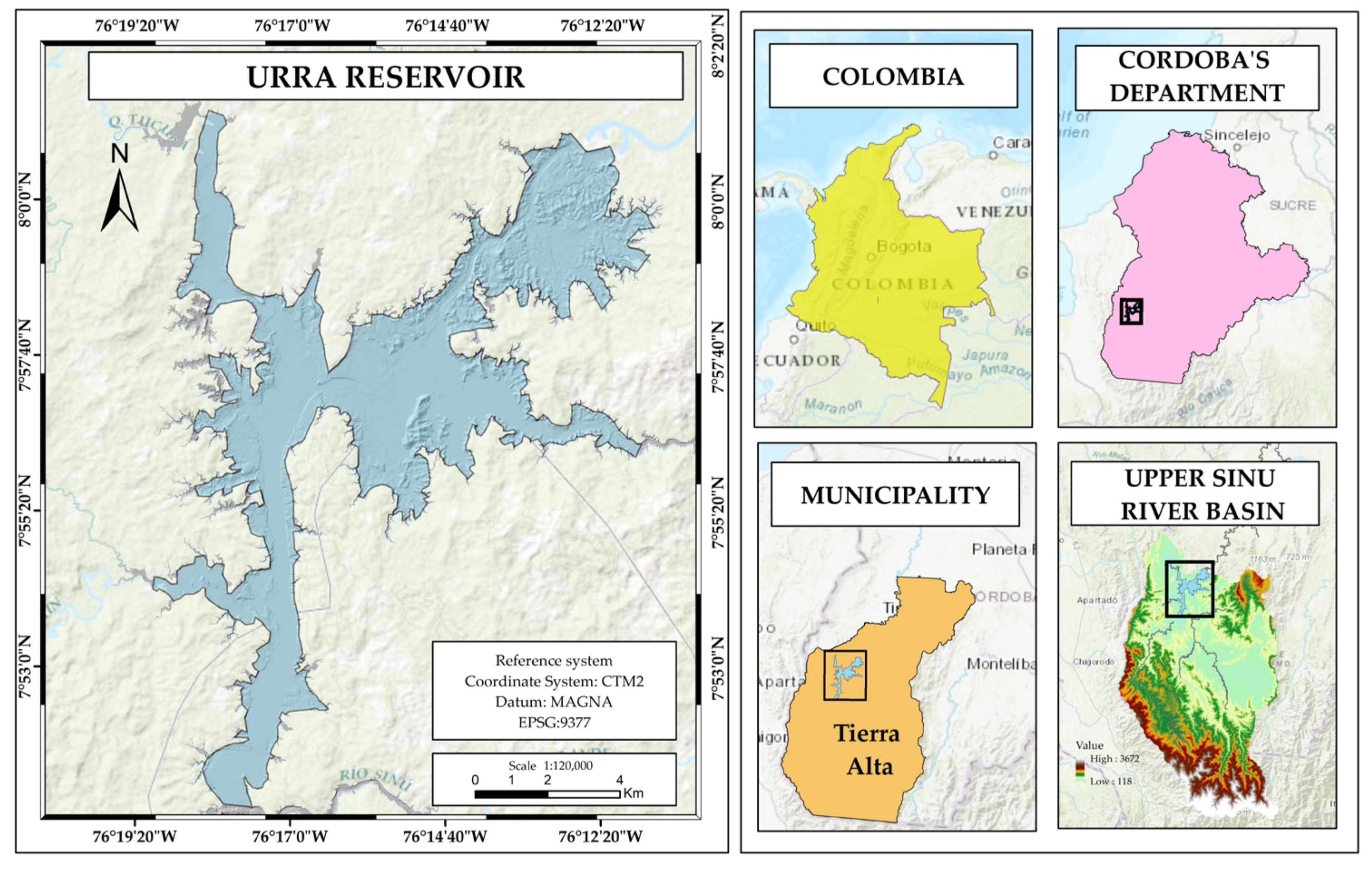
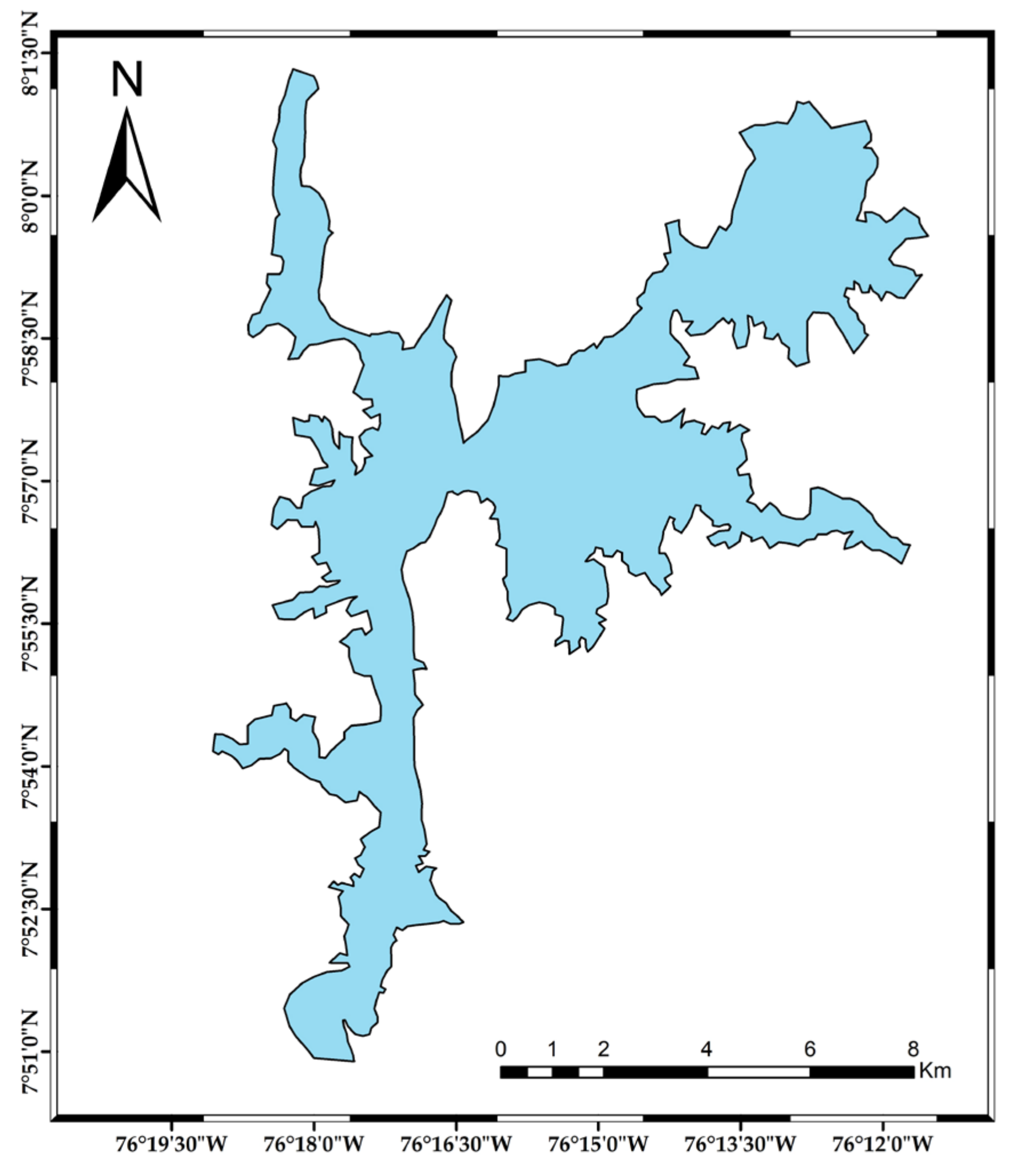
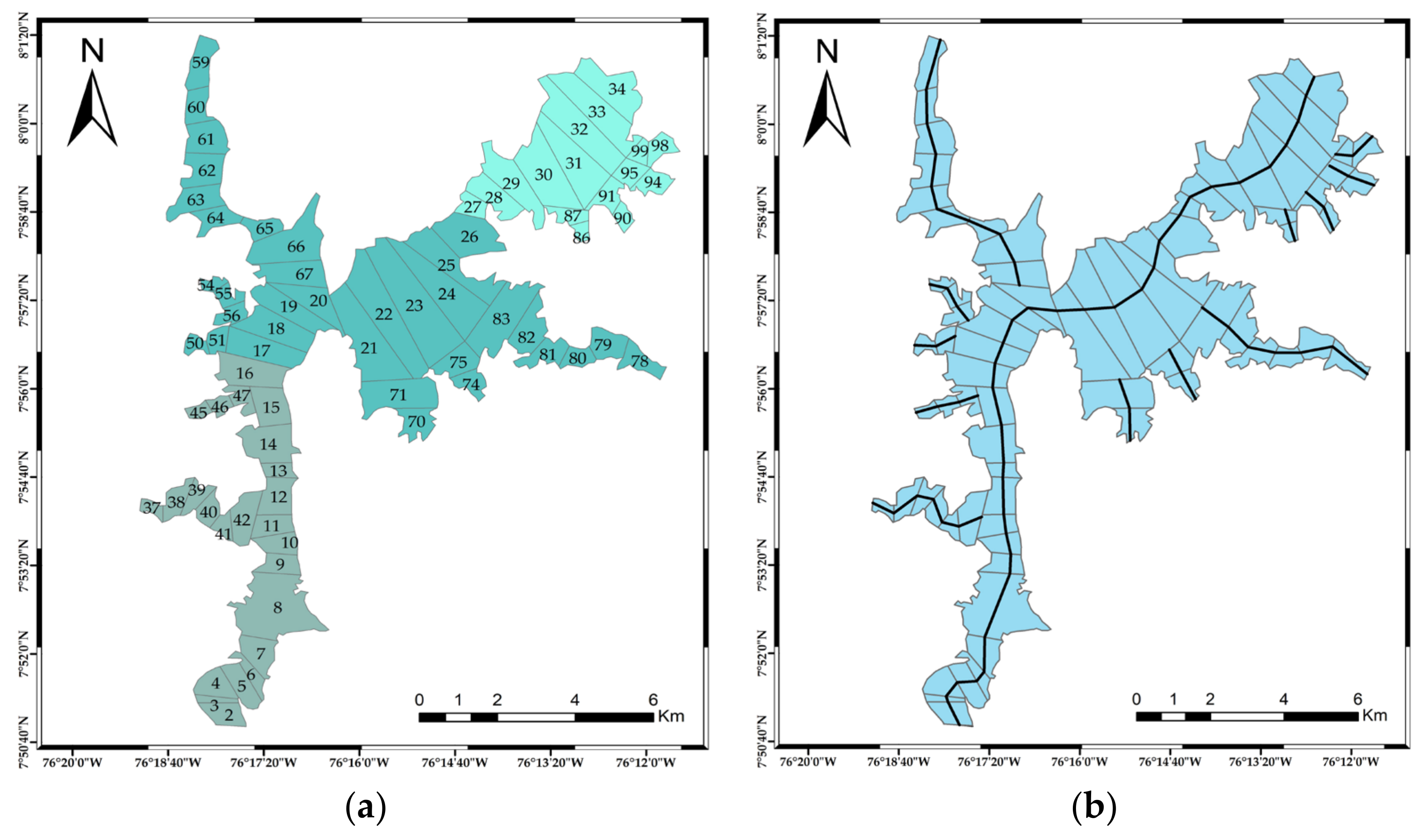
2.1. Study Area

URRÁ reservoir, built in 2009, is located in northwestern Colombia, 30 km south of the municipality of Tierralta in the Department of Córdoba. The Sinú River (with its tributaries, the Manso and Esmeralda Rivers) and the Verde River are its main inflows, originating in the Paramillo National Natural Park. [41]. Its 45 km length allows it to cross the Embera Katio indigenous reserves of the Alto Sinú region. The maximum discharge capacity is 700 m³/s, and the flow rate at which flooding begins downstream of the dam is 775 m³/s [42].

The reservoir has an overflow located on the right bank of the river with a maximum discharge capacity of 9500 m³/s. The reservoir inundation area is 274 km², with a total volume of 1740 × 10⁶ m³ and live storage of 1200 × 10⁶ m³.

On the other hand, the area of the Sinú basin up to the URRÁ dam location is approximately 4600 km², while its total area up to the point where it flows into the Caribbean Sea is 13,952 km². This region is characterized by a tropical rainforest and an altitudinal gradient of 250–1270 m above sea level [43], with a unimodal rainfall distribution pattern and an average annual rainfall exceeding 3200 mm [44]. Its average temperature is 26.5 °C, with variations throughout the year [45,46]. Figure 1 shows the study area.

2.2. Model Description

2.2.1. Initial and Boundary Conditions of the CE-QUAL-W2 Model

The initial conditions are the hydrochemical and environmental conditions that describe the system’s state at a given point in time prior to the start of the simulation. In the case of a reservoir or reservoir simulation model, the initial conditions include [21]:

• Depth: the average depth and spatial distribution of depth in the reservoir. These values were assigned using the CSV file described in the input and processing data Section 2.2.4.
• Temperature: the average temperature and spatial temperature distribution in the reservoir water. This input was manually assigned as described in the input and processing data Section 2.2.4.
• Salinity: the average and spatial distribution of salinity in the reservoir water.
• Nutrient concentration: This condition describes the concentration of nutrients such as nitrogen and phosphorus and their spatial distribution in the reservoir. Dissolved oxygen concentrations were defined by the modelers.
• Suspended matter concentration: This input defines the suspended matter concentration in the reservoir water and its spatial distribution.
• Flow velocity and direction: The velocity and direction of flow in the reservoir or impoundment.

Boundary conditions are the constraints defined at the boundaries of the system being modeled. In the case of a reservoir simulation model, boundary conditions include:

• Water inflow and outflow: the amount of water entering and leaving the reservoir or impoundment, including flow to and from rivers or aquifers and evapotranspiration. These values were assigned through a CSV file described in the input and processing data Section 2.2.4.
• Nutrient inflow and outflow: the amount of nutrients entering and leaving the reservoir, including wastewater discharge and agriculture.
• Precipitation: the amount of precipitation falling in the reservoir or impoundment.
• Evapotranspiration: the amount of water that evaporates and transpires in the reservoir or impoundment.
• Heat transfer with air: the amount of heat transferred from the air to the water in the reservoir, which affects water temperature.
• Conditions in the river or aquifer feeding the reservoir: this condition refers to the hydrochemical characteristics in the river or aquifer feeding the reservoir, including depth, temperature, salinity, velocity, and direction, among others.

Initial and boundary conditions are significant because they determine the behavior and results of the simulation and are critical to ensure the accuracy and completeness of the results. Therefore, it is important to monitor and periodically update the initial and boundary conditions to ensure the accuracy and completeness of the simulation.

2.2.2. Equations

The six equations that the CE-QUAL-W2 model solves are summarized in

Table 1. Segmentation of the information.

Zone	Segmentation
Zone 1: the confluence of the Verde River/Sinú River	Branch 1 segments 1 to 16. Branches 2 and 3.
Zone 2: middle zone of the reservoir	Branch 1 segments 17 to 26. Branches from 4 to 9.
Zone 3: near the dam	Branch 1 segments 27 to 35. Branches from 10 to 13.

, where (1) represents the continuity equation; (2) horizontal momentum; (3) vertical momentum; (4) mass conservation equation; (5) free surface determination; and (6) equation of state. These equations are described in [47].

$$\frac{\partial UB}{\partial x}+\frac{\partial WB}{\partial z}=qB$$

(1)

$$\frac{\partial UB}{\partial t}+\frac{\partial UUB}{\partial x}+\frac{\partial WUB}{\partial z}=gBsin s_0+gcos s_{0}B\frac{\partial n}{\partial x}-\frac{gcos s_{0}B }{\rho } {{\displaystyle \int }}_n^z\frac{\partial \rho }{\partial x}dz+\frac{1}{\rho }\frac{\partial B{\tau }_{xx}}{\partial x}+\frac{1}{\rho }\frac{\partial B{\tau }_{xz}}{\partial z}+qB{U}_x$$

(2)

$$0=gcos s_0-\frac{1}{\rho }\frac{\partial P}{\partial z}$$

(3)

$$\frac{\partial B\mathsf{\Phi }}{\partial t}+\frac{\partial UB\mathsf{\Phi }}{\partial x}+\frac{\partial WB\mathsf{\Phi }}{\partial z}-\frac{\partial \left(B{D}_x\frac{\partial \mathsf{\Phi }}{\partial x}\right)}{\partial x}-\frac{\partial \left(B{D}_z\frac{\partial \mathsf{\Phi }}{\partial z}\right)}{\partial z}=q_{\mathsf{\Phi }}B+S_{\mathsf{\Phi }}B$$

(4)

$$B_n\frac{\partial n}{\partial t}=\frac{\partial }{\partial x}{{\displaystyle \int }}_n^{h}UBdz+{{\displaystyle \int }}_n^{h}qBdz$$

(5)

$$\rho =f\left(T_w,{\phi }_{TDS,}{\phi }_{ss}\right)$$

(6)

where U = velocity in the horizontal direction; B = width of the water body; x = horizontal direction; W = speed in the vertical direction; z = vertical direction; q = lateral flow per unit width; t = time; g = gravity acceleration; α = slope of the channel with the horizontal; ρ = density; P = pressure; 𝜏x = mean lateral shear stress in the x-direction; 𝜏z = mean lateral shear stress in the z-direction; η = elevation to the free surface; h = water depth; f(TW, ΦTDS, ΦSS) = function of density depending on water temperature, total dissolved solids or salinity, and suspended inorganic solids; qΦ = lateral mass flow (inlet/outlet) of the constituent per unit volume; SΦ = kinetic term of the constituent; Φ = concentration of the constituent (lateral mean); Dx = coefficient of dispersion of constituents in the longitudinal direction; Dz = coefficient of diffusion of constituents in the vertical direction.

2.2.3. Generalities

The simulation performed used version 4.5 of the CE-QUAL-W2 software. The model must be calibrated and validated with data measured in the area to generate reliable and accurate results. The description below includes geometric data, the initial and boundary conditions, the main parameters of the water quality model, and constants referring to the model [48,49]. It is essential to mention that the model does not establish the option of reservoirs, which is why the body water type was specified as a lake, considering the similarities in behaviors and characteristics. Another fundamental piece of information was to provide the dimensions of the outlet hydraulic structure (spillway) for the model to recognize the dynamics in the system. For this study, the slope assumed a constant value of 0 for the entire reservoir. Data dates were converted to Julian days, and it was assumed that the sampling was held at 12:00:00 p.m.; therefore, the first day of January is denoted as Julian day 1.5. File preparation was carried out using ArcGIS version 10.8 software.

Time configuration for the simulation year started from 20 January to 3 December 2010. For 2019, it began on 30 January and ended on 4 December. The validation was run for 2020, making it possible to show that the model could simulate events on a different date. These years were selected according to data availability and to evaluate two different climatic conditions, 2010, with a remarkable La Niña phenomenon, and 2019, with the El Niño phenomenon at the beginning of the cycle. The year 2020 was selected to calibrate the model.

2.2.4. Input and Processing Data

As a first step, the study area was delimited (Figure 2) through a shapefile layer between the upstream zone “confluence of the Sinú River/Verde River” to the downstream zone “near the dam”. Some ramifications were disparaged because they were unrepresentative when compared with the main ones of the total area of the body of water.

Once delimited, it was necessary to divide the body of water into grids of vertical and longitudinal dimensions, allowing complete coverage of the mass of water in the direction of the flow since both the hydrodynamic and water quality analyses of the model CE-QUAL-W2 work based on the finite difference method [50]. Each segment had several vertical layers with the same heights; the tool used to develop the length and direction of each segment was ArcGIS COGO, recorded in other studies [40]. Following that, a total of 100 segments originated (Figure 3a), 74 were real, and 26 functioned as border conditions, indicating where each branch begins and ends; a total of 13 branches were classified (Figure 3b), and the confluence zone between the Verde River and the Sinú River was established as the entrance of the reservoir.

Storage volume calculation for each segment was done using the “Polygon Volume” tool of ArcGIS, where the height of the cross sections was 1 m, to obtain accurate results and a good calculation time.

The width of each vertical layer was determined assuming a block geometry for the DEM (digital elevation model, with 1.0 m of resolution) in TIN format with one (1) m resolution. Seventy vertical layers originated, including two extra layers at the top and bottom of the bathymetric model as boundary conditions, with altitudes from 72 to 140 m.a.s.l.

Previously calculated data such as segment length, direction, and cell width were used for creating the bathymetry file in CSV (comma-separated values) format (an essential element for developing the computational grid for the W2 model) [51]. Initial water elevation was set as 125.6 m.a.s.l. on 20 January 2010 (the start of the simulation), and the Manning coefficient was set at 0.035 for the entire bottom of the reservoir.

As a consideration for the bathymetry, when the cell widths were above 1 m, they were increased to 5 m. At the same time, the values below the 1 m threshold were eliminated as they were insignificant and generated instability in the model.

For the temperature parameter, the frequency of data collection was 3 days for each month of the year. From the surface, the measurements were taken every 0.50 m up to 7 m, every meter up to 15 m, and every 3 m for the remaining depth. The sampling procedure was carried out by a laboratory authorized by IDEAM (Institute of Hydrology, Meteorology, and Environmental Studies). Since there were three zones (1—confluence of the Verde River/Sinú River, 2—middle zone of the reservoir, and 3—near the dam) from which to obtain the data, they were distributed strategically for each segment and branch, as specified in Table 1. The chosen values for all branches corresponded to Julian days 1.5 and 337.5.

As for the flow rate, defined as inflow and outflow, daily data were chosen for branch 1, i.e., from Julian day 1.5 to 365.5, while for the remaining branches (12 branches), the values chosen were just the ones for Julian days 1.5 and 365.5, assuming an inflow rate equal to 0.

The meteorological boundary conditions, defined as external driving forces that affect the reservoir dynamics [37] required in the model, were dew point temperature, wind direction and speed, air temperature, and cloudiness. Information for 2010 came from a weather station (IDEAM code: 13015040), while for 2019, parameters such as wind speed and direction resulted from analyzing the information provided by the MERRA-2 reanalysis.

The water quality parameters entered into the model are shown in

Table 2. Water quality parameters.

Parameter	Unit
Temperature	(°C)
Dissolved oxygen	(mg/L)

.

2.2.5. Calibration and Sensitivity Analysis

Sensitivity analysis, also known as hypothetical analysis, allows us to determine which input parameters significantly influence the model response [52]. Temperature and dissolved oxygen were chosen as the main variables to be modeled, as in other studies, due to their significant influence on the reservoir’s chemical state [50]. Temperature can accelerate the different chemical reactions, and dissolved oxygen indicates how the reservoir is in relation to the dynamics of organic matter. DO also provides information about aquatic ecosystem health [53,54,55,56].

The iterative process to conduct this analysis [57] consisted of modifying each of the parameters shown in

Table 3. Parameters selected to perform the temperature sensitivity analysis.

Description	Parameters	Unity	−50%	−20%	Calibration Range	20%	50%
Eddy longitudinal viscosity	AX	m2s−1	0.5	0.8	1.0	1.2	1.5
Eddy longitudinal diffusivity	DX	m2s−1	0.5	0.8	1.0	1.2	1.5
Manning’s coefficient	FRICT	m2s−1	0.015	0.024	0.030	0.036	0.045
Wind shelter coefficient	WSC	-	0.2	0.32	0.4	0.48	0.6
Absorbed solar radiation at the surface	BETA	-	0.21	0.33	0.45	0.50	0.63
Absorption coefficient for pure water	EXH2O	m−1	0.375	0.6	0.75	0.9	1.125
Heat exchange coefficient in the sediment	CBHE	W m−2s−1	0.25	0.4	0.5	0.6	0.75

Note: The calibration range value was set with limits (±20, 50%).

and verifying the magnitude of the reaction provoked concerning the observed variation in the results.

The goodness-of-fit and the errors between the observed and simulated data were evaluated quantitatively through the mean square error statistical index (RMSE) and mean absolute error (AME), which was considered because it is directly interpretable and applied in multiple studies [7,11,58].

2.2.6. Source of Errors

It is worth mentioning that there are different types of errors: those coming from the field information report, from the digital elevation models, from the absence of meteorological information data, outlier data, and even those intrinsic to the CE-QUAL-W2 model as it is parameterized by default for subtropical lakes.

3. Results and Discussion

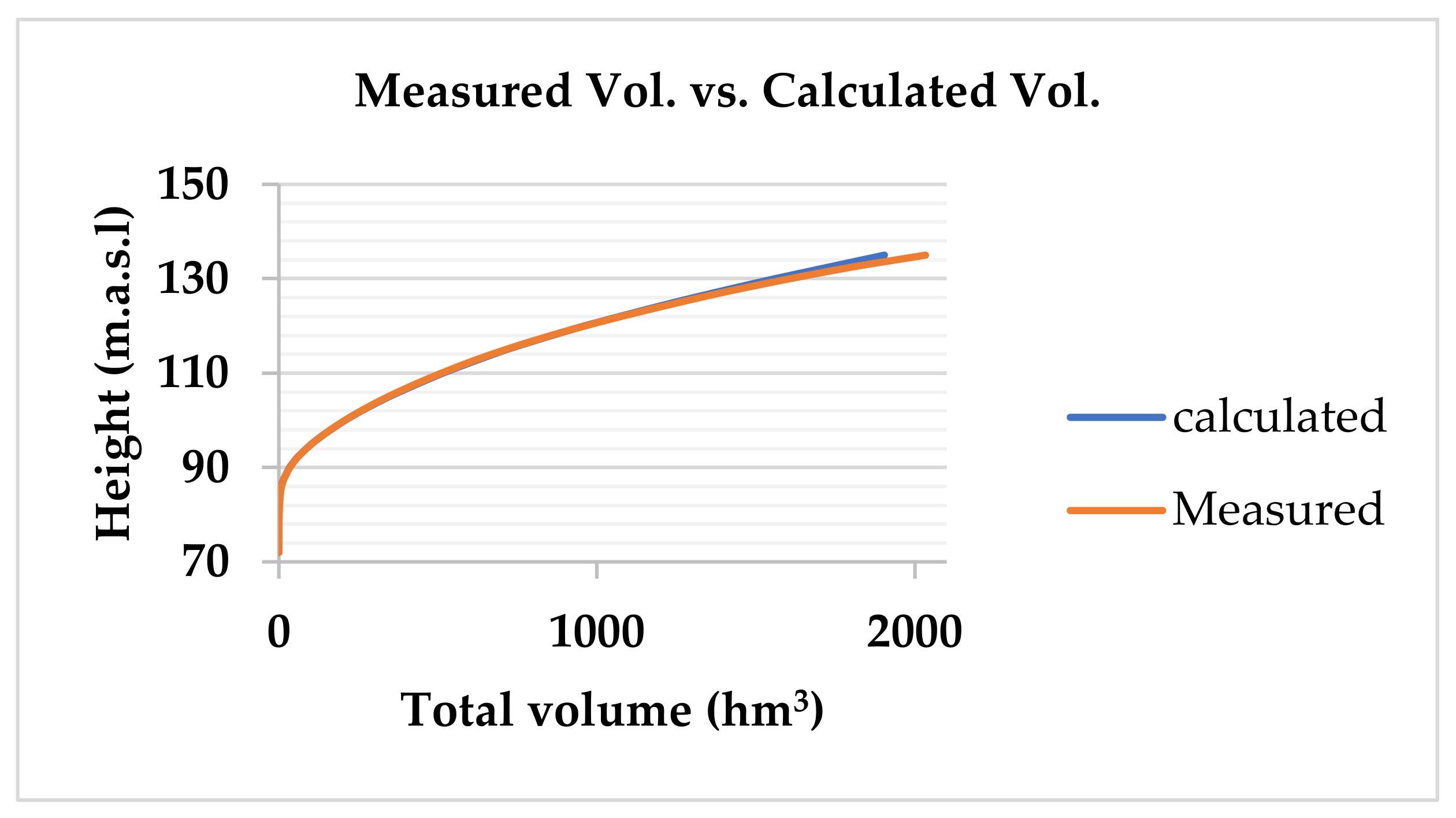
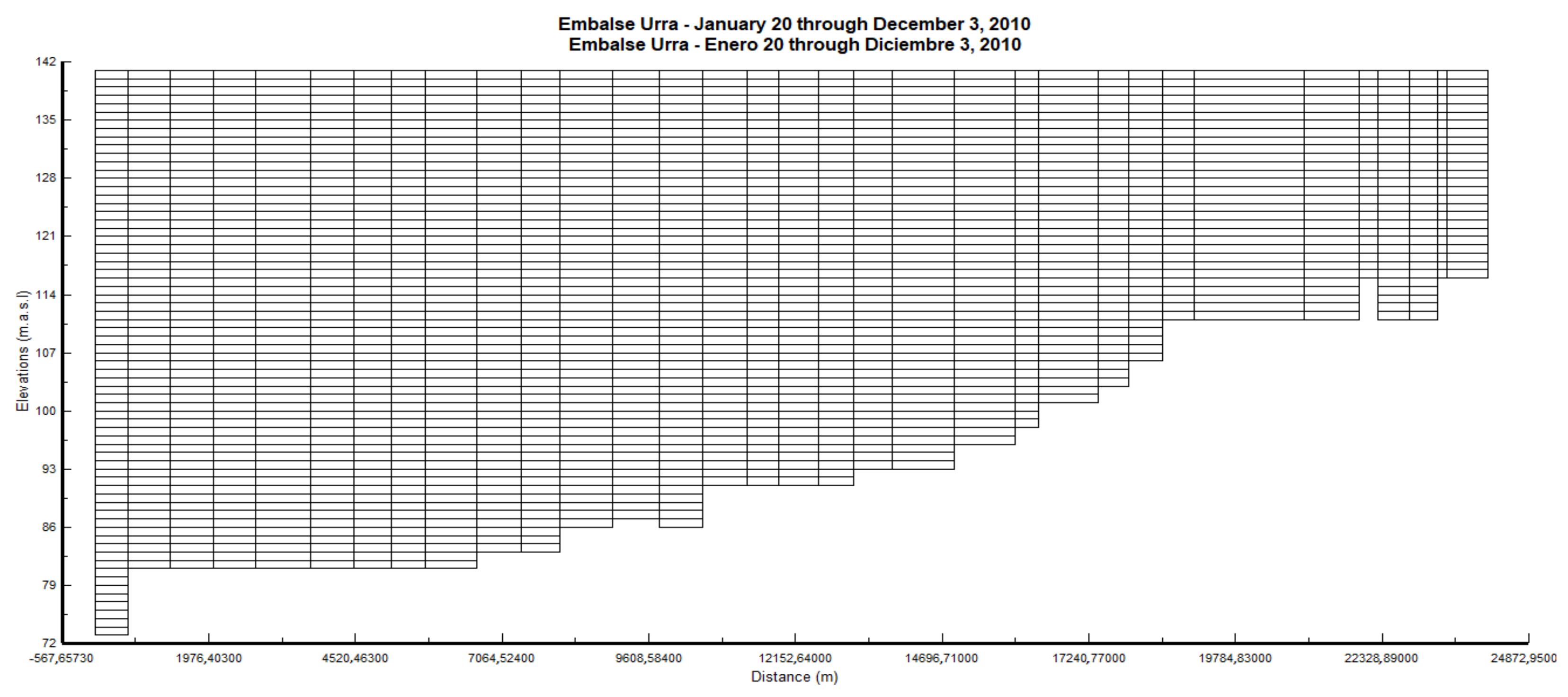
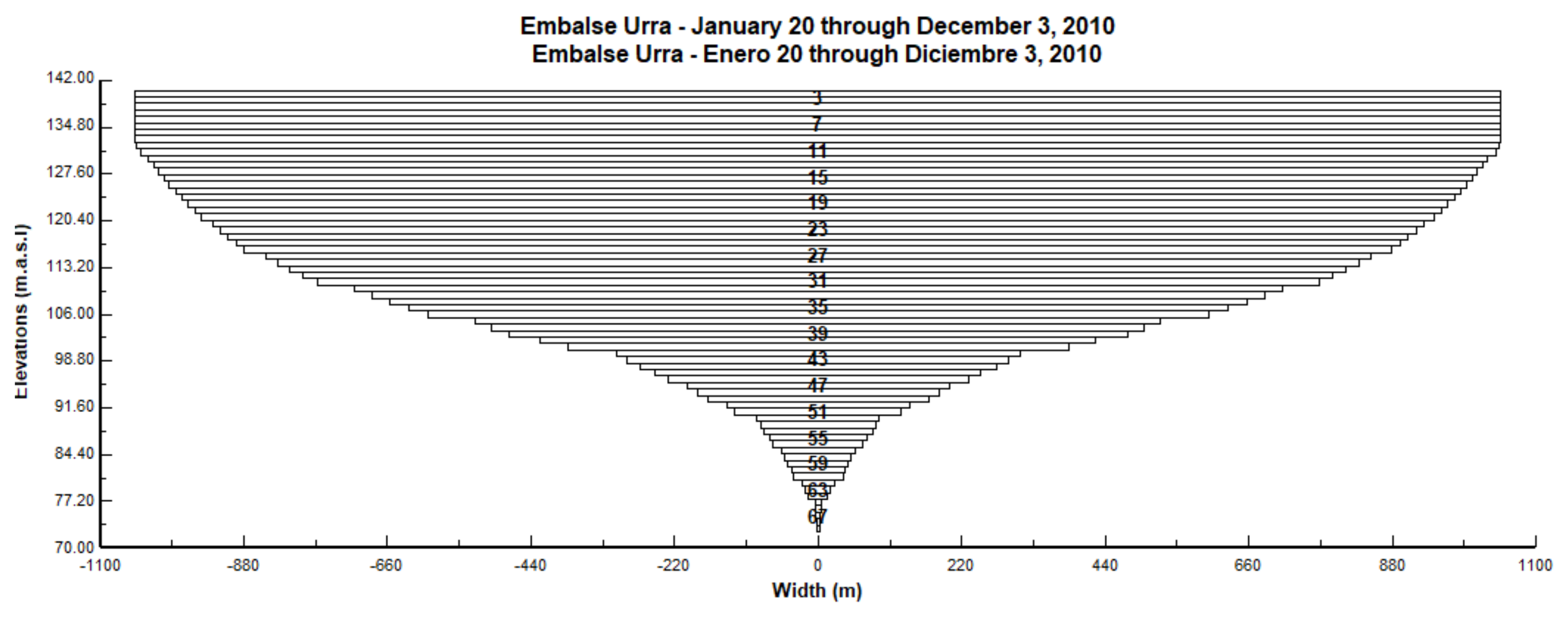
3.1. Analysis of the Bathymetry Results

The volume estimated through layers in ArcGIS was accurate, obtaining a correlation coefficient (R²) of 0.99 and NSE of 0.998, indicating a height/volume curve (Figure 4) similar to actual data. The model has also generated optimal results in previous studies by showing that the simulated water surface elevations are similar to the observed data set [29,50].

It is essential to point out that the number of segments (100) and the thickness of the vertical pipes are determining factors for accurate morphometry of the reservoir, which is why specific cell widths were adjusted (cells with values close to zero were eliminated) to avoid instability in the model in order to achieve more representative simulations.

In the Nechako reservoir study assessing the period 1979–2017, the volume and timing of total simulated inflows in the main tributaries presented a bias of 16% and NSE of 0.53 originating from the underestimation of peak flows during high years and runoff from streams and small tributaries not considered by the model. For the study, this may relate to the actual morphometry of the water body [28]. In contrast, other studies have shown good agreement between observed and simulated stored water elevation curves [26].

The longest segment in this research had a value of 1900.9 m, and the shortest was 168.2 m. Figure 5 shows the bathymetric profile of branch 1 for the reservoir, and Figure 6 displays the vertical bathymetry of segment 34 (branch 1 near the dam), where greater depths (of the dam) were found, reaching layer 69 of the bathymetric model.

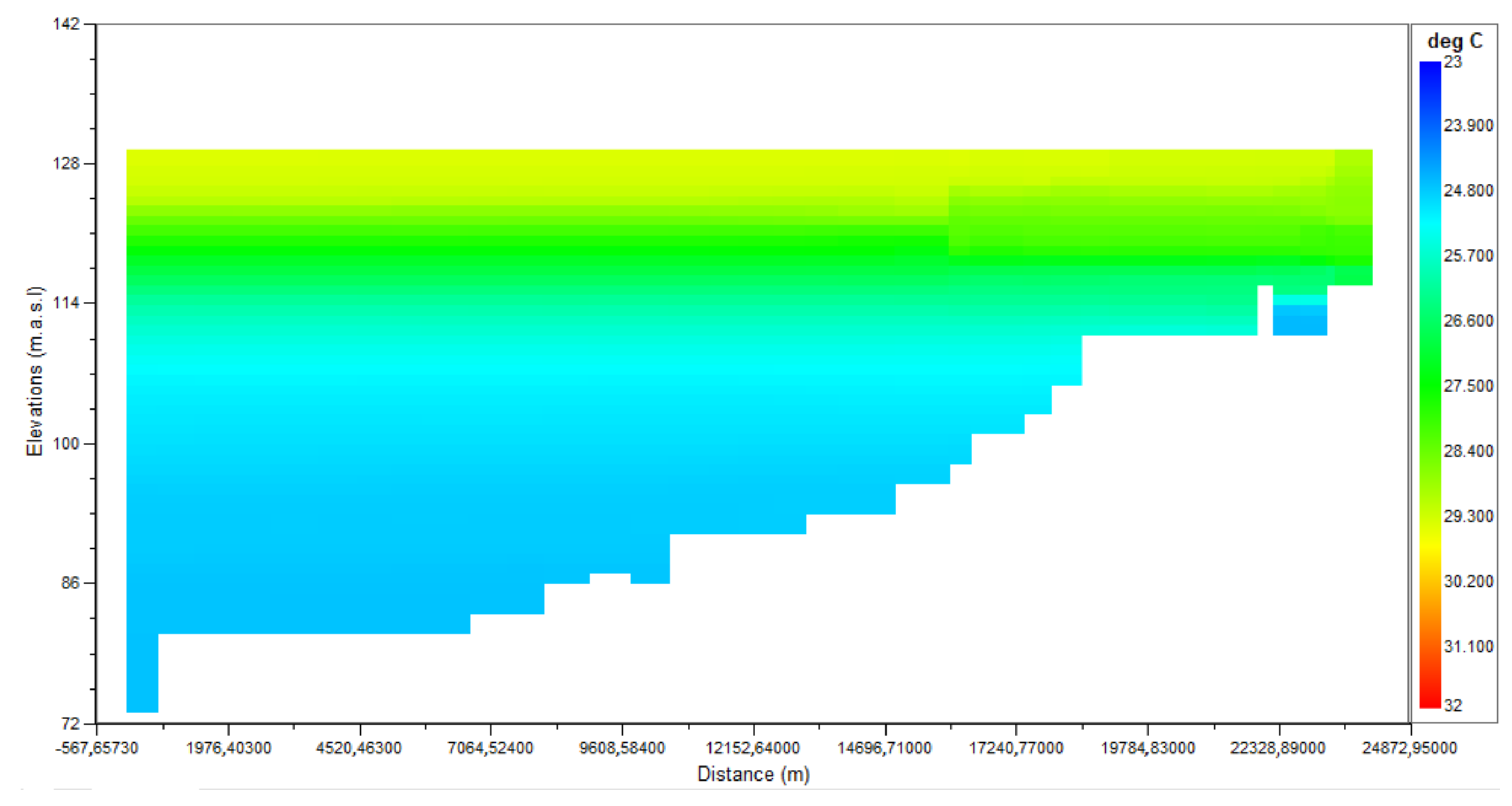
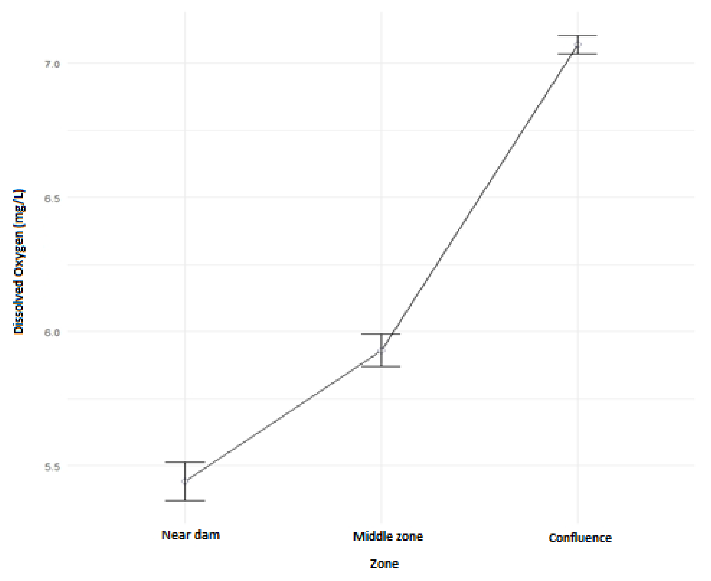
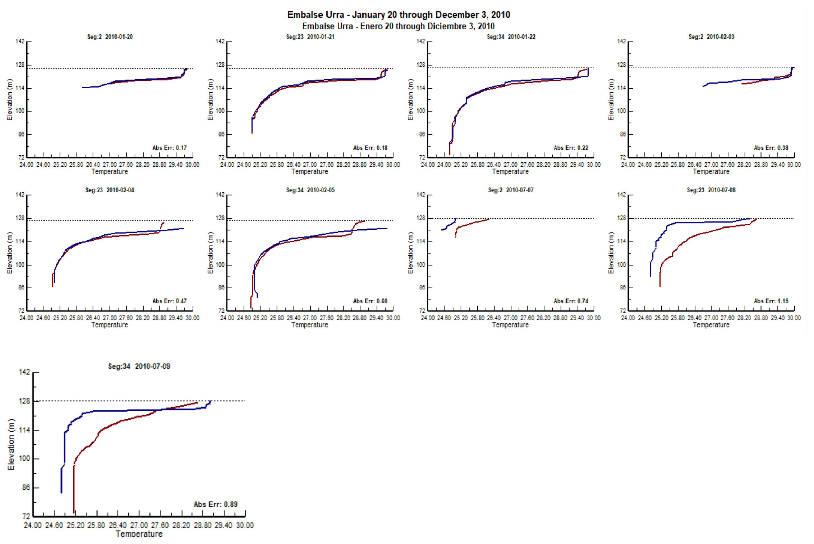
3.2. Water Quality Simulation

The statistical analysis results show that 90% of the surface temperature of the sampling area is above 29.79 °C for the year 2019, which agrees with the model simulation results after calibration (Figure 7) and the monitoring data presented by Winton et al. [8]. The adequate representation of the seasonal progression of the surface temperature has been evidenced in other studies, such as the studies of the Nechako [28] and Soyanggang [59] reservoirs.

In the middle zone and near the dam, the surface area presents high values due to low mobility and high retention; this observation was also reported by Azadi et al. (2021) [60]. Other studies have shown strong correlations between air temperature and water temperature [36]. The vertical behavior of this variable is coherent since it generally decreases as depth increases. Thus, the warmest layers are found near the surface, while the coldest occur in lower regions (e.g., the epilimnion, thermocline, and hypolimnion) [61,62]. Thermal stratification has been recorded at a depth of 3.6 m in many reservoirs where layers with different temperatures are formed [63].

A greater instability was expected in the confluence zone between the Verde and Sinú Rivers, where the large upstream inflow momentum creates a well-mixed condition, as shown in other studies [36]. However, statistics and calibration showed the opposite; the temperature behavior was observed to be more homogeneous in this zone, which may be because the warmer and lighter inflowing water traps the colder and denser water. Before the inflow was cold enough to submerge below the epilimnion, the deepening of the thermocline had already reached the bottom of the reservoir, consequently ending the stratification [36].

On the other hand, the areas of greatest instability occurred near the dam. Their origin may be due to the variation of conditions in the different depths (Figure 8); it is worth mentioning that wind speed and light penetration are the main factors that affect temperature stratification in reservoirs [37].

The fact that there are fewer data points in the deeper layers causes the dissolved oxygen data to be underestimated. On the other hand, in the confluence zone, this parameter did not show a significant difference, with a possible explanation being the re-aeration process caused by the movement of the inflowing water [64].

In the middle zone, there is a significant difference in the dissolved oxygen concentration in the first meters. In contrast, from 4 to 24 m, it tends to have similar behavior because, in the upper layers, there is greater movement due to aeration, as mentioned by Simons [65], who explained that there are other variables with a greater influence on DO concentration, such as wind, and that inflows and outflows are not the main factors that determine water circulation patterns.

Figure 9 shows a comparison of average dissolved oxygen by zone. The model results exhibit a narrower range compared to the measurements reported by Winton et al. [8].

At times of the year with high rainfall, Figure 10 shows how dissolved oxygen concentrations change at greater depths in the middle zone and near the dam (left side of Figure 10), the water temperature at the inlet of the reservoir decreases and due to the difference in density, these water reaches the deeper areas of the reservoir which increase dissolved oxygen [66].

Calibration

The trial-and-error technique was applied, considering that the values given for the calibration cannot show conditions far from the behavior and characteristics present in reality.

The first step was the calibration of the wind shelter coefficient (WSC), and this parameter represents the adjustment of the wind reaching the water body since the terrain surrounding the reservoirs protects the water body, so the winds observed at the weather stations are usually different. WSC takes values from 0 to 1; the higher the value, the greater the effects of wind on the water body [67]. In this research, after five adjustments, the chosen one was 0.4 for the 2010 calibration. Previous studies varied the wind shelter coefficient from 0.5 to 0.9 for mountainous and dense vegetation canopy and 1.0 for open terrain. This parameter is deemed the most significant effect on temperature during calibration [33].

As shown in Figure 11, in almost all of the first 6 months, the mean absolute error was below 1.

The eddy’s longitudinal viscosity (AX) was set in 1 as the default value (Figure 12). This value was also the best fit for the calibration process, as indicated by previous research [37]. This parameter and eddy longitudinal diffusivity (DX) are related to the dispersion of heat and constituents in the longitudinal axis but have little effect on the vertical heat dispersion.

On the other hand, the absorption coefficient for pure water (EXH2O) obtained the best fit at 0.75 (75%) (Figure 13). In previous studies [37], EXH2O has been considered a key parameter as it can affect the vertical heat exchange and directly determine the ability of shortwave solar radiation to penetrate the water layer, directly influencing the water temperature and then influencing the hydrodynamics [26].

In the “eddy viscosity” section, the vertical turbulence was adjusted, being TKE (turbulent kinetic energy) according to the software recommendation (Figure 14). However, after testing this method, a mean absolute error of 0.557 was obtained, while the W2 method gave an error of 0.552. Then, the W2 method was chosen because it presented a better fit for deep and stratified water bodies.

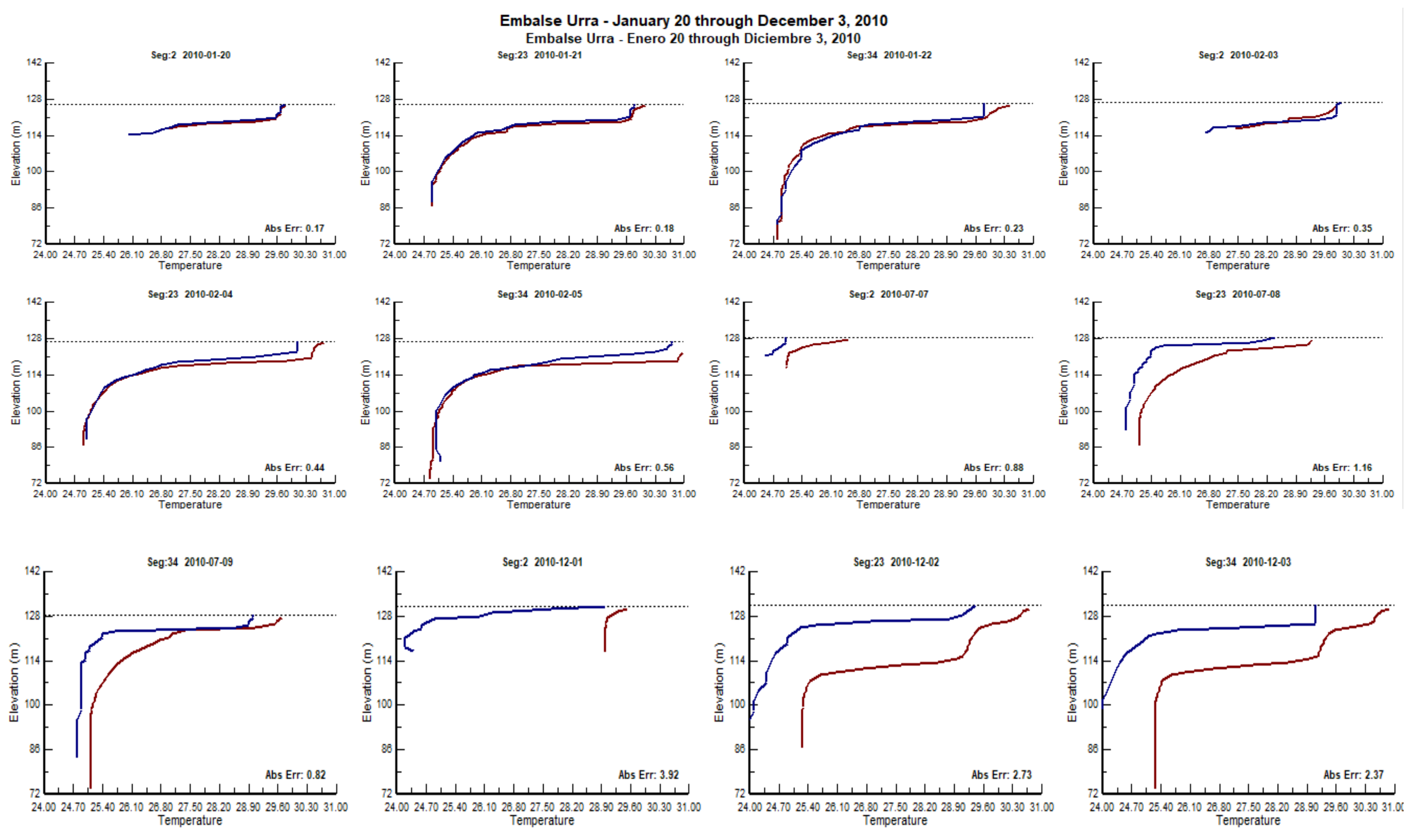
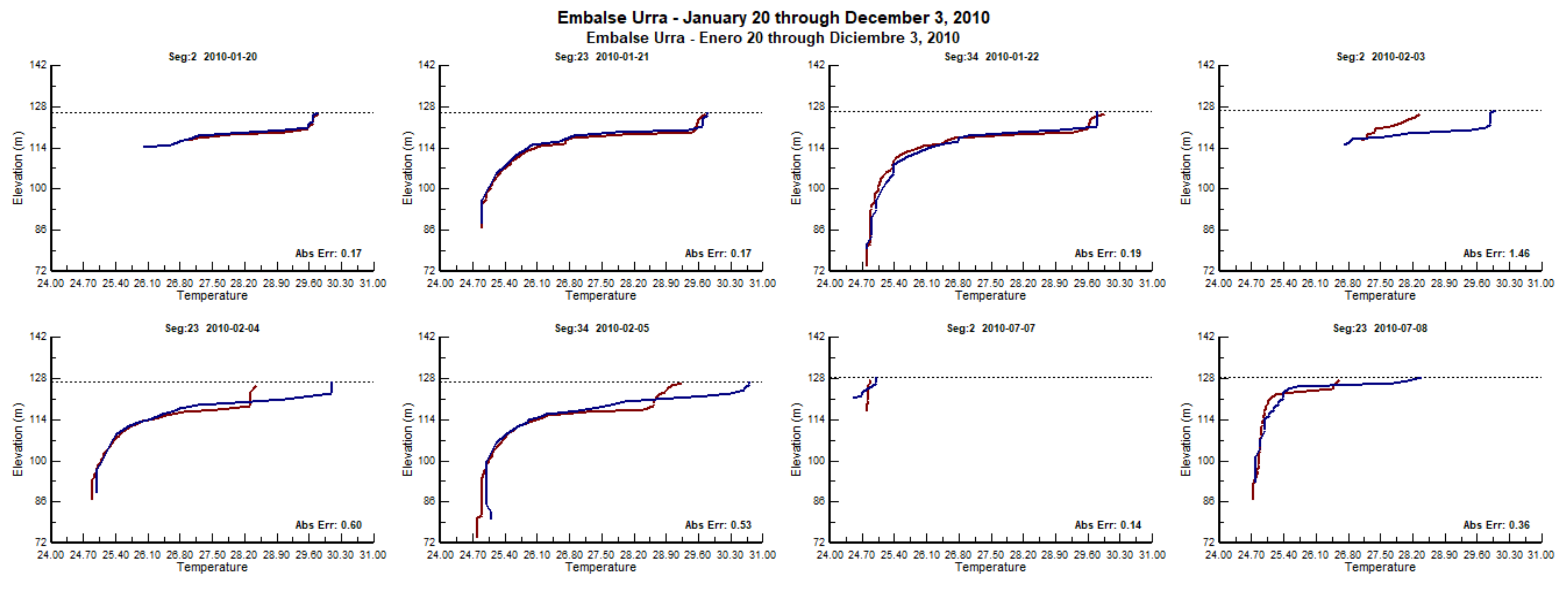
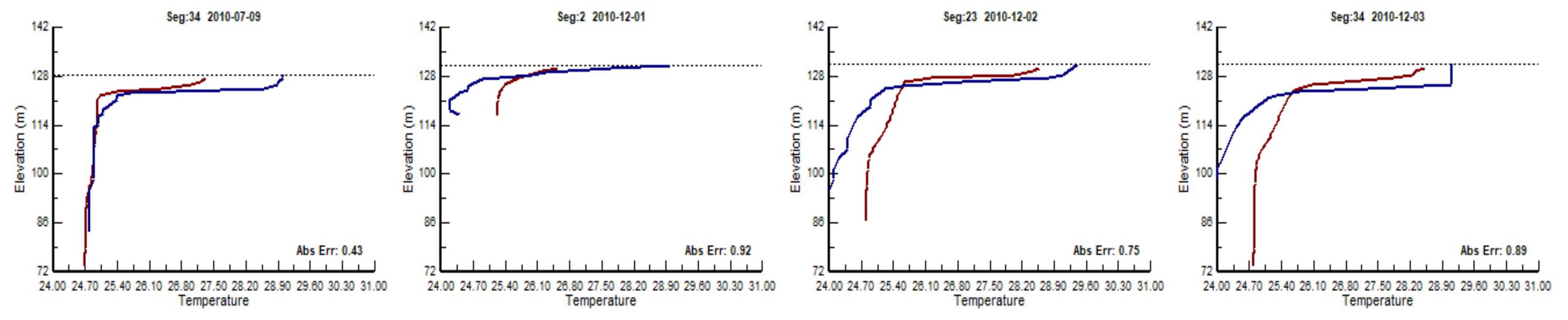
3.3. Results with Adjusted Meteorology (Applying the Vertical Turbulence Method W2)

Air temperature, dew point temperature, wind direction and speed, and cloudiness data were adjusted (Figure 15). All these values were taken from the weather station except for the dew point temperature, calculated from the relative humidity and air temperature. These estimated values decrease the accuracy of the meteorological data considering that the model suggests hourly data frequency (24 h). Authors such as Cole [68] have indicated that the absence of meteorological data, especially wind data, collected at the water body site significantly contributes to errors between measured and calculated temperatures.

In the year’s second half, modeled values significantly differed from actual-world conditions, so it was necessary to continue adjusting some variables. The main difficulty corresponds to meteorological data.

A dew point temperature (TDEW) value of 23 °C was set as the average for the whole year, and the water temperature at the inlet (TIN) was taken as the average confluence temperature for the whole vertical water column. Modifying the TDEW value did not produce adequate results, but TIN did.

2010 Calibration: Finally, the meteorology was adjusted with interpolation (TDEW adjusted with interpolation from air temperature data with relative humidity), and TIN was taken as the average confluence temperature for the entire water column, thus obtaining the best calibration result (mean absolute error of 0.552). The other coefficients were the same as those previously assigned.

The meteorology was adjusted (Figure 16) depending on the reservoir monitoring sampling, and the time the samples were taken. Finally, the data were interpolated to know the wind direction and speed.

2019 Calibration: To calibrate the year 2019, the same coefficients and parameters established in 2010 were used with the same values, except for WSC, which was modified to 0.90. On the other hand, meteorological data such as wind speed and direction were taken from the MERRA-2 reanalysis since there are no nearby stations with records for 2019. The calibration value obtained was 0.864.

3.4. Model Validation

The validation was performed to verify the accuracy and optimal applicability of the model within the established ranges for reservoir water quality. In addition, it allowed verification that the calibration performed was satisfactory and that the results presented a low uncertainty.

The validation was carried out for 2020 with the same parameters chosen for the 2019 calibration (hydraulic parameters, coefficients, calculation algorithms) to verify that the model corresponds to the reservoir conditions. As meteorological and hydrological variables are different between years, 2020 climate data were used for validation.

It should be noted that IDEAM did not record wind direction data and some meteorological variables for this period, so they were taken from the MERRA-2 reanalysis instead. The authors must warn the readers that the accuracy in the variable data sets of reanalysis models, such as MERRA-2, has to be tested through performance metrics as they are subject to significant biases in their estimation [69].

Table 4. Final coefficients and meteorology adjusted for validation.

HEAT EXCHANGE	WB1
H SLHTC—Heat computations/Equilibrium (ET) or Term-by-term (TERM)	TERM
SROC—Read in short wave solar radiation ON or OFF	OFF
RHEVAP—Use Ryan-Harleman evap model—for cooling ponds ON or OFF	OFF
METIC—Interpolate meteorological data ON or OFF	OFF
FETCHC—Heinz Stefan lake fetch correction—there is already an internal OFF	OFF
AFW—Evaporation coefficient	9.2
BFW—Evaporation coefficient	0.46
CFW—Evaporation coefficient	2
WINDH—Wind height measurement above the ground surface, m	10
TRANSPORT SCHEME	WB1
SLTRC—UPWIND, QUICKEST, ULTIMATE—use ULTIMATE	ULTIMATE
THETA—degree of implicitness—use 0.55—Time-weighting for vertical adv	0.55
HYD COEFFICIENTS	WB1
AX—Longitudinal eddy viscosity, m2/s	1
DX—Longitudinal eddy diffusivity/conductivity, m2/s	1
CBHE—Coefficient of bottom heat exchange, W m−1 oC−1	0.5
TSED—Temperature of sediment, C, average year-round air temperature	25
Fl—Interfacial friction factor	0
TSEDF—Sediment temperature coefficient (0–1) heat lost to sediments th	0.8
FRICC—Bottom friction factor type: CHEZY or MANN	MANN
ZO—water surface roughness height, m, for wind shear	0.001

shows the results of the interpolation-adjusted meteorology (TDEW) of the 2010 calibration. The sediment temperature was set at 25 °C. The absolute validation error was 0.676, which is within the acceptable range of the model.

4. Conclusions

The hydrodynamic and two-dimensional water quality model, CE-QUAL-W2, was employed to evaluate the URRÁ reservoir in Colombia. Model calibration was carried out by adjusting different parameters after each model run to allow the simulated results to be as close as possible to those observed. The parameters included longitudinal eddy viscosity, longitudinal eddy diffusivity, Manning coefficient, wind sheltering coefficient, solar radiation absorbed on the surface layer, absorption coefficient of pure water, and heat exchange coefficient in sediments. Temperature and dissolved oxygen were the variables modeled due to their importance in the ecology of water bodies. The sensitivity analysis for the simulation years 2010, 2019, and 2020 yielded mean absolute errors of 0.552, 0.864, and 0.676, respectively. The results show warming and cooling trends in the surface and bottom layers of the reservoir, respectively.

The model outcomes evidence an excellent fit between the simulated and observed data; this consistency is meaningful when providing reliable information. A calibrated model can help to forecast strategies to improve water quality.

Further research must be focalized to link water quality dynamic with microbiological parameters (phytoplankton and zooplankton) using the CE-QUAL-W2 software to predict algal blooms.

References

1. Stelzer, C.; Nestmann, F. The importance of reservoirs for water supply and power generation—An overview. In Global Change: Enough Water for All?: Scientific Facts; Verlag Wissenschaftliche Auswertungen: Hamburg, Germany, 2007; Volume 5, pp. 117–121. [Google Scholar] [CrossRef]
2. Branche, E. The multipurpose water uses of hydropower reservoir: The SHARE concept. C. R. Phys. 2017, 18, 469–478. [Google Scholar] [CrossRef]
3. Li, J.; Zhong, P.-A.; Wang, Y.; Yang, M.; Fu, J.; Liu, W.; Xu, B. Risk analysis for the multi-reservoir flood control operation considering model structure and hydrological uncertainties. J. Hydrol. 2022, 612, 128263. [Google Scholar] [CrossRef]
4. Boretti, A.; Rosa, L. Reassessing the projections of the World Water Development Report. Npj Clean Water 2019, 2, 15. [Google Scholar] [CrossRef] [Green Version]
5. United Nations, U.W. Wastewater Management A UN-Water Analytical Brief; WHO: Geneva, Switzerland, 2015. [Google Scholar]
6. Khodabandeh, F.; Dehghani Darmian, M.; Azhdary Moghaddam, M.; Hashemi Monfared, S.A. Reservoir quality management with CE-QUAL-W2/ANN surrogate model and PSO algorithm (case study: Pishin Dam, Iran). Arab. J. Geosci. 2021, 14, 401. [Google Scholar] [CrossRef]
7. Noori, R.; Yeh, H.-D.; Ashrafi, K.; Rezazadeh, N.; Bateni, S.M.; Karbassi, A.; Kachoosangi, F.T.; Moazami, S. A reduced-order based CE-QUAL-W2 model for simulation of nitrate concentration in dam reservoirs. J. Hydrol. 2015, 530, 645–656. [Google Scholar] [CrossRef]
8. Winton, R.S.; López-Casas, S.; Valencia-Rodríguez, D.; Bernal-Forero, C.; Delgado, J.; Wehrli, B.; Jiménez-Segura, L. Patterns and drivers of water quality changes associated with dams in the Tropical Andes. EGUsphere 2022, 403, 1–21. [Google Scholar] [CrossRef]
9. Song, Y.; You, L.; Chen, M.; Li, J.; Zhang, L.; Peng, T. Key hydrodynamic principles for controlling algal blooms using emergency reservoir operation strategies. J. Environ. Manag. 2023, 325, 116470. [Google Scholar] [CrossRef]
10. Lehner, B.; Liermann, C.R.; Revenga, C.; Vörösmarty, C.; Fekete, B.; Crouzet, P.; Döll, P.; Endejan, M.; Frenken, K.; Magome, J.; et al. High-resolution mapping of the world’s reservoirs and dams for sustainable river-flow management. Front. Ecol. Environ. 2011, 9, 494–502. [Google Scholar] [CrossRef] [Green Version]
11. Afshar, A.; Shojaei, N.; Sagharjooghifarahani, M. Multiobjective Calibration of Reservoir Water Quality Modeling Using Multiobjective Particle Swarm Optimization (MOPSO). Water Resour. Manag. 2013, 27, 1931–1947. [Google Scholar] [CrossRef]
12. Chanudet, V.; Fabre, V.; van der Kaaij, T. Application of a three-dimensional hydrodynamic model to the Nam Theun 2 Reservoir (Lao PDR). J. Great Lakes Res. 2012, 38, 260–269. [Google Scholar] [CrossRef]
13. Neitsch, S.; Arnold, J.; Kiniry, J.; Williams, J.; King, K. Soil and Water Assessment Tool (SWAT) User’s Manual Version 2000; Technical Report for Texas Water Resources Institute: College Station, TX, USA, 2002. [Google Scholar]
14. Ma, L.; He, C.; Bian, H.; Sheng, L. MIKE SHE modeling of ecohydrological processes: Merits, applications, and challenges. Ecol. Eng. 2016, 96, 137–149. [Google Scholar] [CrossRef]
15. Xingpo, L.; Muzi, L.; Yaozhi, C.; Jue, T.; Jinyan, G. A comprehensive framework for HSPF hydrological parameter sensitivity, optimization and uncertainty evaluation based on SVM surrogate model—A case study in Qinglong River watershed, China. Environ. Model. Softw. 2021, 143, 105126. [Google Scholar] [CrossRef]
16. Dehdari, V.; Oliver, D.S.; Deutsch, C.V. Comparison of optimization algorithms for reservoir management with constraints—A case study. J. Pet. Sci. Eng. 2012, 100, 41–49. [Google Scholar] [CrossRef]
17. Diogo, P.A.; Fonseca, M.; Coelho, P.S.; Mateus, N.S.; Almeida, M.C.; Rodrigues, A.C. Reservoir phosphorous sources evaluation and water quality modeling in a transboundary watershed. Desalination 2008, 226, 200–214. [Google Scholar] [CrossRef]
18. Hamilton, D.P.; Hocking, G.C.; Patterson, J.C. Criteria for selection of spatial dimension in the application of one- and two-dimensional water quality models. Math. Comput. Simul. 1997, 43, 387–393. [Google Scholar] [CrossRef]
19. Ochoa, S.; Reyna, T.; Reyna, S.; García, M.; Labaque, M.; Manuel Díaz, J. Modelación Hidrodinámica Del Tramo Medio Del Río Ctalamochita, Provincia de Córdoba. Rev. Fac. Cienc. Exactas Fís. Nat. 2016, 3, 95–101. [Google Scholar]
20. Ostfeld, A.; Salomons, S. A hybrid genetic—Instance based learning algorithm for CE-QUAL-W2 calibration. J. Hydrol. 2004, 310, 122–142. [Google Scholar] [CrossRef]
21. Wells, S.A. CE-QUAL-W2: A Two-Dimensional, Laterally Averaged, Hydrodynamic and Water Quality Model, Version 4.2.2. User Manual: Part 1 Introduction, Model Download Package, How to Run the Model; Technical Report for Department of Civil and Environmental Engineering Portland State University: Portland, OR, USA, 2020. [Google Scholar]
22. Bonalumi, M.; Anselmetti, F.S.; Wüest, A.; Schmid, M. Modeling of temperature and turbidity in a natural lake and a reservoir connected by pumped-storage operations. Water Resour. Res. 2012, 48, W08508. [Google Scholar] [CrossRef] [Green Version]
23. Noori, R.; Tian, F.; Ni, G.; Bhattarai, R.; Hooshyaripor, F.; Klöve, B. ThSSim: A novel tool for simulation of reservoir thermal stratification. Sci. Rep. 2019, 9, 18524. [Google Scholar] [CrossRef] [Green Version]
24. Noori, R.; Asadi, N.; Deng, Z. A simple model for simulation of reservoir stratification. J. Hydraul. Res. 2019, 57, 561–572. [Google Scholar] [CrossRef]
25. Tavoosi, N.; Hooshyaripor, F.; Noori, R.; Farokhnia, A.; Maghrebi, M.; Kløve, B.; Haghighi, A.T. Experimental-numerical simulation of soluble formations in reservoirs. Adv. Water Resour. 2022, 160, 104109. [Google Scholar] [CrossRef]
26. Chuo, M.; Ma, J.; Liu, D.; Yang, Z. Effects of the impounding process during the flood season on algal blooms in Xiangxi Bay in the Three Gorges Reservoir, China. Ecol. Model. 2018, 392, 236–249. [Google Scholar] [CrossRef]
27. Kurup, R.G.; Hamilton, D.P.; Phillips, R.L. Comparison of two 2-dimensional, laterally averaged hydrodynamic model applications to the Swan River Estuary. Math. Comput. Simul. 2000, 51, 627–638. [Google Scholar] [CrossRef]
28. Larabi, S.; Schnorbus, M.A.; Zwiers, F. A coupled streamflow and water temperature (VIC-RBM-CE-QUAL-W2) model for the Nechako Reservoir. J. Hydrol. Reg. Stud. 2022, 44, 101237. [Google Scholar] [CrossRef]
29. Shojaei, N.; Wells, S. Automatic Calibration of Water Quality Models for Reservoirs and Lakes. In Proceedings of the World Environmental and Water Resources Congress 2014, Portland, OR, USA, 1–5 June 2014; Volume 2014, pp. 1020–1029. [Google Scholar] [CrossRef]
30. American Society of Civil Engineers Task Committee on Turbulence Models in Hydraulic Computation. Turbulence Modeling of Surface Water Flow and Transport: Part I. J. Hydraul. Eng. 1988, 114, 970–991. [Google Scholar] [CrossRef]
31. Afshar, A.; Feizi, F.; Yousefi Moghadam, A.; Saadatpour, M. Enhanced CE-QUAL-W2 model to predict the fate and transport of volatile organic compounds in water body: Gheshlagh reservoir as case study. Environ. Earth Sci. 2017, 76, 803. [Google Scholar] [CrossRef]
32. Bartholow, J.; Hanna, R.B.; Saito, L.; Lieberman, D.; Horn, M. Simulated Limnological Effects of the Shasta Lake Temperature Control Device. Environ. Manag. 2001, 27, 609–626. [Google Scholar] [CrossRef]
33. Chung, S.; Oh, J. Calibration of CE-QUAL-W2 for a monomictic reservoir in a monsoon climate area. Water Sci. Technol. 2006, 54, 29–37. [Google Scholar] [CrossRef]
34. Deliman, P.N.; Gerald, J.A. Application of the Two-Dimensional Hydrothermal and Water Quality Model, CE-QUAL-W2, to the Chesapeake Bay–Conowingo Reservoir. Lake Reserv. Manag. 2002, 18, 10–19. [Google Scholar] [CrossRef] [Green Version]
35. Azadi, F.; Ashofteh, P.-S.; Loáiciga, H.A. Reservoir Water-Quality Projections under Climate-Change Conditions. Water Resour. Manag. 2018, 33, 401–421. [Google Scholar] [CrossRef]
36. Xie, Q.; Liu, Z.; Fang, X.; Chen, Y.; Li, C.; MacIntyre, S. Understanding the Temperature Variations and Thermal Structure of a Subtropical Deep River-Run Reservoir before and after Impoundment. Water 2017, 9, 603. [Google Scholar] [CrossRef] [Green Version]
37. Zhao, L.; Cheng, S.; Sun, Y.; Zou, R.; Ma, W.; Zhou, Q.; Liu, Y. Thermal mixing of Lake Erhai (Southwest China) induced by bottom heat transfer: Evidence based on observations and CE-QUAL-W2 model simulations. J. Hydrol. 2021, 603, 126973. [Google Scholar] [CrossRef]
38. Yu, S.J.; Lee, J.Y.; Ha, S.R. Effect of a seasonal diffuse pollution migration on natural organic matter behavior in a stratified dam reservoir. J. Environ. Sci. 2010, 22, 908–914. [Google Scholar] [CrossRef] [PubMed]
39. Torres, E.; Galván, L.; Cánovas Ruiz, C.; Soria-Píriz, S.; Arbat-Bofill, M.; Nardi, A.; Papaspyrou, S.; Ayora, C. Oxycline formation induced by Fe(II) oxidation in a water reservoir affected by acid mine drainage modeled using a 2D hydrodynamic and water quality model—CE-QUAL-W2. Sci. Total. Environ. 2016, 562, 1–12. [Google Scholar] [CrossRef]
40. Parra-Cuadros, M.; Villegas-Jiménez, N.E.; Hernández-Atilano, E.; Aguirre-Ramírez, N.J.; de Vélez-Macías, F.J. Aplicación del modelo CE QUAL-W2: Una aproximación a la estructura térmica en el embalse Miguel Martínez Isaza, Concordia, Antioquia, Colombia. Tecnológicas 2019, 22, 99–113. [Google Scholar] [CrossRef] [Green Version]
41. Clavijo-Bernal, O.F. El agua y la participación como ejes articuladores del territorio. Consideraciones a partir de URRÁ y su incidencia sobre la cuenca del río Sinú. Gestión Ambiente 2021, 24, 51–74. [Google Scholar] [CrossRef]
42. URRÁ S.A. E.S. Reporte técnico de monitoreo ambiental. Printed document. 2021. [Google Scholar]
43. Hernández Camacho, J.; Walschburger, T.; Ortiz Quijano, R.; Hurtado Guerra, A. Origen y Distribución de La Biota Su-ramericana y Colombiana. Acta Zool. Mex. 1992, 55–104. [Google Scholar]
44. Palencia Severiche, G.; Mercado-Fernandez, T.; Combath Caballero, E. Estudio Agroclimático de Córdoba; Technical Report for Facultad de Ciencias Agrícolas; Universidad de Córdoba: Córdoba, Spain, 2006. [Google Scholar]
45. URRÁ S.A. E.S. Incremento del volumen del embalse de URRÁ. Reporte técnico. 2010. [Google Scholar]
46. Vélez Flórez, A.J. Propuesta Metodológica Para La Evaluación y Cuantificación de La Alteración Del Régimen de Caudales de Corrientes Alteradas Antrópicamente, Caso URRÁ I. Master’s Thesis, Universidad Nacional de Colombia, Bogotá, Colombia, 2009. [Google Scholar]
47. Wells, S.A. CE-QUAL-W2: A Two-Dimensional, Laterally Averaged, Hydrodynamic and Water Quality Model, Version 4.5, User Manual Part 2, Hydrodynamic and Water Quality Model Theory; Technical Report for Department of Civil and Environmental Engineering, Portland State University: Portland, OR, USA, 2021. [Google Scholar]
48. Kuo, J.-T.; Lung, W.-S.; Yang, C.-P.; Liu, W.-C.; Yang, M.-D.; Tang, T.-S. Eutrophication modelling of reservoirs in Taiwan. Environ. Model. Softw. 2006, 21, 829–844. [Google Scholar] [CrossRef]
49. Yang, Y.; Deng, Y.; Tuo, Y.; Li, J.; He, T.; Chen, M. Study of the thermal regime of a reservoir on the Qinghai-Tibetan Plateau, China. PLoS ONE 2020, 15, e0243198. [Google Scholar] [CrossRef]
50. Debele, B.; Srinivasan, R.; Parlange, J.-Y. Coupling upland watershed and downstream waterbody hydrodynamic and water quality models (SWAT and CE-QUAL-W2) for better water resources management in complex river basins. Environ. Model. Assess. 2006, 13, 135–153. [Google Scholar] [CrossRef]
51. Dolz, J.; Armengol, J.; Roura, M.; De Pourcq, K.; Arbat, M.; López, P. Estudio de La Dinámica Sedimentaria y Batimetría de Precisión Del Embalse de Ribarroja. 2009.
52. Chakraborty, S.; Chowdhury, R. A hybrid approach for global sensitivity analysis. Reliab. Eng. Syst. Saf. 2016, 158, 50–57. [Google Scholar] [CrossRef]
53. Almansa, C.; Masaló, I.; Reig, L.; Piedrahita, R.; Oca, J. Influence of tank hydrodynamics on vertical oxygen stratification in flatfish tanks. Aquac. Eng. 2014, 63, 1–8. [Google Scholar] [CrossRef]
54. Barrut, B.; Blancheton, J.-P.; Champagne, J.-Y.; Grasmick, A. Mass transfer efficiency of a vacuum airlift—Application to water recycling in aquaculture systems. Aquac. Eng. 2012, 46, 18–26. [Google Scholar] [CrossRef] [Green Version]
55. Null, S.E.; Mouzon, N.R.; Elmore, L.R. Dissolved oxygen, stream temperature, and fish habitat response to environmental water purchases. J. Environ. Manag. 2017, 197, 559–570. [Google Scholar] [CrossRef]
56. Zhang, Y.; Wu, Z.; Liu, M.; He, J.; Shi, K.; Zhou, Y.; Wang, M.; Liu, X. Dissolved oxygen stratification and response to thermal structure and long-term climate change in a large and deep subtropical reservoir (Lake Qiandaohu, China). Water Res. 2015, 75, 249–258. [Google Scholar] [CrossRef]
57. Liu, W.-C.; Chen, W.-B.; Kimura, N. Impact of phosphorus load reduction on water quality in a stratified reservoir-eutrophication modeling study. Environ. Monit. Assess. 2008, 159, 393–406. [Google Scholar] [CrossRef]
58. Shabani, A.; Zhang, X.; Chu, X.; Zheng, H. Automatic Calibration for CE-QUAL-W2 Model Using Improved Global-Best Harmony Search Algorithm. Water 2021, 13, 2308. [Google Scholar] [CrossRef]
59. Kim, S.K.; Choi, S.-U. Assessment of the impact of selective withdrawal on downstream fish habitats using a coupled hydrodynamic and habitat modeling. J. Hydrol. 2021, 593, 125665. [Google Scholar] [CrossRef]
60. Azadi, F.; Ashofteh, P.-S.; Chu, X. Evaluation of the effects of climate change on thermal stratification of reservoirs. Sustain. Cities Soc. 2021, 66, 102531. [Google Scholar] [CrossRef]
61. Boehrer, B.; Schultze, M. Stratification of Lakes. Rev. Geophys. 2008, 46, RG2005. [Google Scholar] [CrossRef] [Green Version]
62. Prats, J.; Reynaud, N.; Rebière, D.; Peroux, T.; Tormos, T.; Danis, P.-A. LakeSST: Lake Skin Surface Temperature in French inland water bodies for 1999–2016 from Landsat archives. Earth Syst. Sci. Data 2018, 10, 727–743. [Google Scholar] [CrossRef] [Green Version]
63. Koparan, C.; Koc, A.B.; Sawyer, C.; Privette, C. Temperature Profiling of Waterbodies with a UAV-Integrated Sensor Subsystem. Drones 2020, 4, 35. [Google Scholar] [CrossRef]
64. Owen, L.; Dávalos Lind, L. An Introduction to the Limnology of Lake Chapala, Jalisco, Mexico. In The Lerma-Chapala Watershed; Springer: Boston, MA, USA, 2001. [Google Scholar]
65. Simons, T.J. Effect of Outflow Diversion on Circulation and Water Quality of Lake Chapala; National Water Research Institute: Fountain Valley, CA, USA, 1984. [Google Scholar]
66. Arbat Bofill, M.; Bladé, E.; Sánchez Juny, M.; Cea, L.; Niñerola, D.; Dolz, J. Modelación Numérica 3d Hidrodinámica y Térmica En El Entorno de La Confluencia Ebro-Segre. In Proceedings of the Libro Artículos XXVII Congreso Latinoamericano de Hidráulica, Lima, Peru, 26–30 September 2016; pp. 3888–3897. [Google Scholar]
67. Kim, Y.; Kim, B. Application of a 2-Dimensional Water Quality Model (CE-QUAL-W2) to the Turbidity Interflow in a Deep Reservoir (Lake Soyang, Republic of Korea). Lake Reserv. Manag. 2006, 22, 213–222. [Google Scholar] [CrossRef]
68. Cole, T. Reservoir Thermal Modeling Using CE-QUALW2. In Development and Application of Computer Techniques to Environmental Studies VIII; WIT Press: Southampton, UK, 2000; pp. 238–246. [Google Scholar]
69. Vega-Durán, J.; Escalante-Castro, B.; Canales, F.A.; Acuña, G.J.; Kaźmierczak, B. Evaluation of Areal Monthly Average Precipitation Estimates from MERRA2 and ERA5 Reanalysis in a Colombian Caribbean Basin. Atmosphere 2021, 12, 1430. [Google Scholar] [CrossRef]
Figure 1. Study area.
Water 15 01013 g001
Figure 2. Study area delimitation.
Water 15 01013 g002
Figure 3. Segmentation of the water body. (a) Enumerated segmentation. (b) Segmentation showing the number of branches represented by the black lines, where branch 1 is the longest.
Water 15 01013 g003
Figure 4. Measured volume vs. calculated volume.
Water 15 01013 g004
Figure 5. Bathymetric profile of branch 1. The maximum water level in the reservoir is 172 m, while 72 is the minimum water level near the reservoir.
Water 15 01013 g005
Figure 6. Vertical profile of segment 34.
Water 15 01013 g006
Figure 7. Simulation for 14 February 2019. February was selected because it has less precipitation and better represents the stratification of the reservoir.
Water 15 01013 g007
Figure 8. Simulation for 15 March 2019. March was selected because it has less precipitation and better represents the stratification of the reservoir. Note: The right side refers to the confluence zone.
Water 15 01013 g008
Figure 9. Comparison of average dissolved oxygen results by zone.
Water 15 01013 g009
Figure 10. Simulation of dissolved oxygen, 2019.
Water 15 01013 g010
Figure 11. Modified wind shelter coefficient (WSC).
Water 15 01013 g011
Figure 12. Eddy longitudinal viscosity (AX).
Water 15 01013 g012
Figure 13. Absorption coefficient of pure water (EXH2O).
Water 15 01013 g013
Figure 14. Adjustment by TKE.
Water 15 01013 g014
Figure 15. Adjustment by the vertical turbulence method W2.
Water 15 01013 g015
Figure 16. Results with adjusted methodology.
Water 15 01013 g016aWater 15 01013 g016b