
Daily Streamflow Forecasts Based on Cascade Long Short-Term Memory (LSTM) Model over the Yangtze River Basin

1
Key Laboratory of Hydrometeorological Disaster Mechanism and Warning of Ministry of Water Resources, Nanjing University of Information Science and Technology, Nanjing 210044, China
2
School of Hydrology and Water Resources, Nanjing University of Information Science and Technology, Nanjing 210044, China
*
Author to whom correspondence should be addressed.
Water 2023, 15(6), 1019; https://doi.org/10.3390/w15061019
Submission received: 2 February 2023
/
Revised: 28 February 2023
/
Accepted: 6 March 2023
/
Published: 7 March 2023
(This article belongs to the Section New Sensors, New Technologies and Machine Learning in Water Sciences)
Abstract
:Medium-range streamflow forecasts largely depend on the accuracy of meteorological forecasts. Due to large errors in precipitation forecasts, most streamflow forecasts based on deep learning rely only on historical data. Here, we apply a cascade Long Short-Term Memory (LSTM) model to forecast daily streamflow over 49 watersheds in the Yangtze River basin for up to 15 days. The first layer of the cascade LSTM model uses atmospheric circulation factors to predict future precipitation, and the second layer uses forecast precipitation to predict streamflow. The results show that the default LSTM model provides skillful streamflow forecasts over most watersheds. At the lead times of 1, 7, and 15 days, the streamflow Kling–Gupta efficiency (KGE) of 78%, 30%, and 20% watersheds are greater than 0.5, respectively. Its performance improves with the increase in drainage area. After implementing the cascade LSTM model, 61–88% of the watersheds show increased KGE at different leads, and the increase is more obvious at longer leads. Using cascade LSTM with perfect future precipitation shows further improvement, especially over small watersheds. In general, cascade LSTM modeling is a good attempt for streamflow forecasts over the Yangtze River, and it has a potential to connect with dynamical meteorological forecasts.
1. Introduction
Under climate change, the frequency and intensity of extreme weather events (e.g., floods, droughts) are likely to increase in many regions [1], and the resulting economic losses and human casualties are also on the rise. Therefore, accurate streamflow forecasting is indispensable for both early warning and mitigation of flood and drought events.
Streamflow forecasting from hydrological models relies heavily on meteorological forcing inputs, all of which are subject to errors and uncertainties. While temperature estimates are often similar between different data products, precipitation estimates often diverge significantly [2,3]. For medium- and long-range streamflow forecast, the skill heavily depends on the quality of the precipitation forecasts [4]. In addition to precipitation (P), evapotranspiration (ET) is more closely related to streamflow than other meteorological variables, such as wind speed or temperature [5], because precipitation and evapotranspiration are the main processes that influence streamflow formation at the basin scale based on a dynamic hydrological balance [6]. In addition, soil moisture (SM) is the initial condition for hydrological forecast, which can affect streamflow by influencing surface infiltration rates and subsurface runoff generation [7,8].
In recent years, deep learning methods were widely used for streamflow forecast. Not only the simple Long Short-Term Memory (LSTM) model, but also a large number of LSTM variants and different machine learning methods coupled with LSTMs are widely used for streamflow forecast and post-processing [9,10,11,12,13]. For example, in the U.S. large sample study (CAMELS) watershed, the performance of streamflow prediction from the LSTM model was better than that from the Sacramento soil moisture accounting model and the NOAA National Water Model with calibrated parameters [14]. In a follow-up study, it was found that even if the trained LSTM model was applied to the ungauged basins, the streamflow prediction performance was still better than that from the above physical models [15]. Compared with traditional linear regression, multilayer perceptron, support vector machine, and other models, the LSTM model also has better performance in daily streamflow predictions [16]. For instance, the LSTM model was used to predict the streamflow in the lead times of 1–30 days (months), and the results show that LSTM was better than the artificial neural network in predicting daily runoff. However, due to the lack of a large number of training data for monthly streamflow, the performance of monthly streamflow prediction was poor [17]. In addition, the LSTM was combined with a Gaussian distribution process model to predict daily streamflow of the Yangtze River basin, and the results show that LSTM was superior to many traditional machine learning models, even for probabilistic streamflow prediction [18]. The LSTM model can also be used for post-processing of the results from a physical model (prediction residual). Some studies showed that using the LSTM model to predict the simulation residual of WRF Hydro can reduce its simulation bias [19].
For deep learning, the data input is very important, such as the accuracy of the data, the type of data, the correlation between the data, etc. In the era of big data, a large amount of data input will lead to the increase in model complexity. How to balance the model complexity and generalization, and how to build a deep learning model with certain interpretability, are very challenging [20]. The LSTM is driven by the historical data to predict streamflow over multiple basins in the United States through data integration. The results show that data integration can not only simplify the historical input of the model, but also extract historical variables more relevant to the target flow, reduce the burden of data input, and improve the prediction performance of the model. It can improve predictions over small watersheds with high autocorrelation of runoff and close rainfall–runoff relationship [21]. In addition to integrating dynamic data, adding static data also proved to improve the streamflow forecasting [18].
In the past, many studies focused on how to preprocess or add various restrictions to the model to achieve skillful streamflow prediction, while how to flexibly use the meteorological prediction data in the streamflow prediction at long lead received less attention. The cascade LSTM predict future meteorological data (e.g., precipitation) firstly, and use it to build a relationship with future streamflow, which is more interpretable than the original LSTM model in a physical manner. The cascade LSTM is also compatible with dynamical meteorological forecasts, which has potential for complementing a dynamical streamflow forecast that is usually carried out by a link hydrological model with meteorological forecasts. However, the application of cascade LSTM is limited to the large uncertainty from meteorological forecasts, which needs a stepwise evaluation.
Furthermore, it is known that model performance decreases with increasing lead times [22,23]. The relationship between decreasing model performance and lead time depends on basin characteristics, such as basin size, land use, geological structure, and quality of hydrometeorological data. For example, compared with smaller watersheds with storm characteristics, large watersheds that require a longer time for river routing can produce better forecasting results [24]. To sum up, the LSTM model and its variants are widely used for streamflow predictions, but most of them are case studies, without comprehensive investigations on the effects of precipitation forecasts on streamflow forecasts over multi-scale basins and multiple lead times. Therefore, comparison among different watersheds and different lead times are necessary to obtain a robust evaluation for the deep learning models.
In this study, we build cascade LSTM models over 49 watersheds in the Yangtze River basin by using synthetic hydrometeorological data from a high-resolution land surface model simulation, and evaluate the streamflow forecast skill with or without a perfect precipitation forecast. We aim to (1) explore the possibility of LSTM models in a streamflow forecast when accurate hydrometeorological data are available, (2) propose a cascade LSTM (the first layer uses meteorological forcings to predict precipitation, and the second layer uses predicted precipitation and related hydrometeorological variables to predict streamflow) to reduce the complexity of the LSTM and improve the generalization, and (3) assess the performance of cascade LSTM streamflow forecasts for different lead time and different watersheds.
2. Materials and Methods
2.1. Study Area and Data
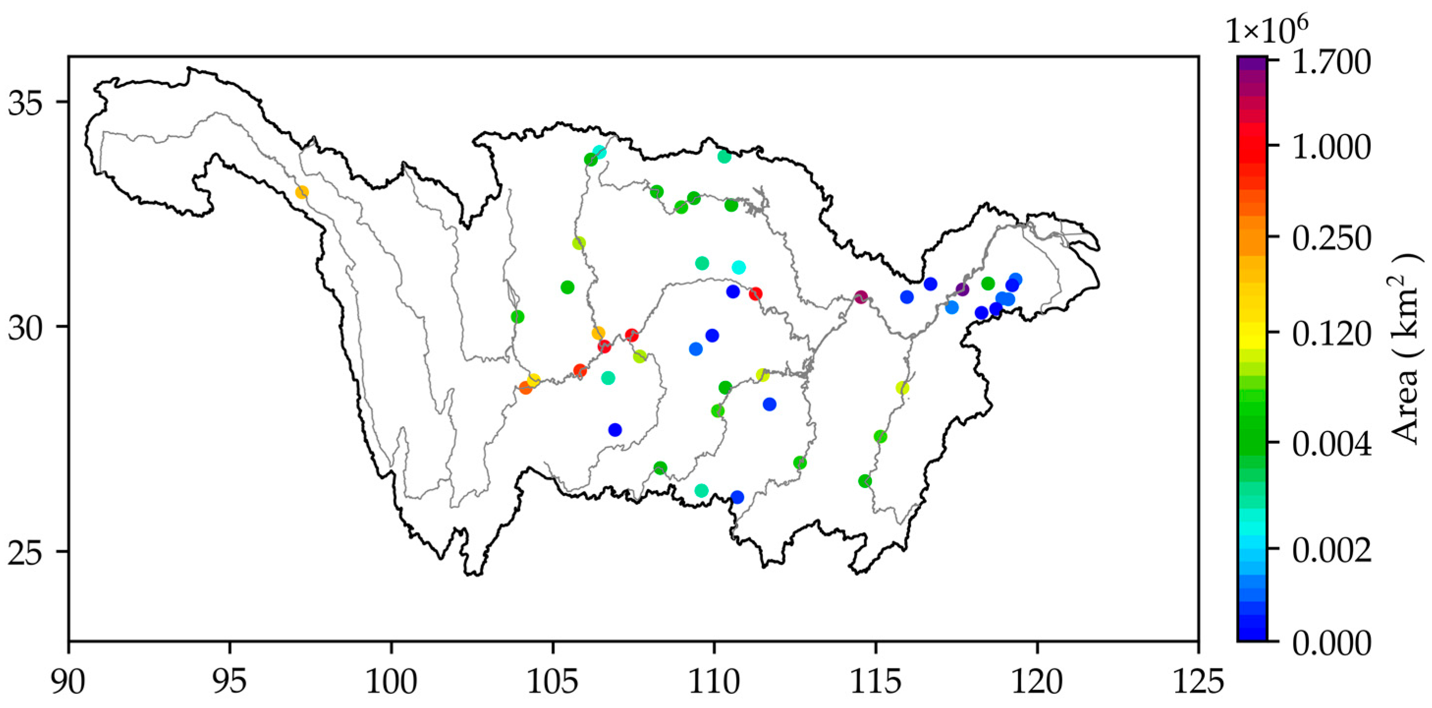
The Yangtze River is the third longest river in the world with a total length of about 6387 km. The water resources of the Yangtze River account for about 36% of China’s total water resources. The Yangtze River basin is located at 90°33′~122°25′ E and 24°30′~35°45′ N, and its area is about 1.8 × 10⁶ km2, which accounts for about 18.8% of China’s total land area. Figure 1 shows the locations of the 49 hydrological stations used in this study. The monthly streamflow observed at these 49 stations was collected from the Yangtze River Basin Hydrological Yearbook published by the Yangtze River Conservancy Commission.
The meteorological forcing data for land surface model simulations are as follows: precipitation was obtained from China Meteorological Administration Land Data Assimilation System (CLDAS) and CN05.1 (uses observations from more than 2000 meteorological stations), and barometric pressure, specific humidity, long and short wave radiation, 2 m temperature, and wind speed were obtained from China Meteorological Forcing Dataset (CMFD) [25]. Surface data include the 1 km resolution global soil texture dataset [26], the 90 m resolution Digital Elevation Model (DEM) from the United States Geological Survey (USGS), the 0.05° resolution GLASS monthly LAI products from 1981 to 1999 [27], and the 2000 to 2017 0.05° resolution MODIS version 6 monthly LAI reprocessing dataset [28]. Due to lack of information, the monthly leaf area index for 1979–1980 is the same as that of 1981 [25]. The geopotential heights used for precipitation forecast in the cascade LSTM were obtained from the fifth generation European ReAnalysis (ERA5) [29].
2.2. The Conjunctive Surface-Subsurface Process Version 2 (CSSPv2) Model
The CSSPv2 model is rooted in the common land model [30], but with improved representations of surface hydrological processes, including the consideration of the quasi three-dimensional soil water transport process [31] and one-dimensional dynamic surface water transport process [32]. Furthermore, some parameterization schemes are adjusted with reference to the common land model v3.5, the one-dimensional groundwater module is added, and the interaction between groundwater and soil water is considered [28]. In addition, the variable infiltration capacity runoff generation scheme, the parameterization of hydraulic properties that considers the impact of soil organic matter, and the soil thermal parameterization scheme are also included in CSSPv2 [8].
The streamflow simulation is mainly based on runoff generation and routing. The infiltration curve is used to represent the distribution of the surface infiltration capacity within the grid, and the shape of the curve is adjusted by parameters to calculate the saturation excess runoff. For the base flow, it relies on the base flow curve. When the soil saturation degree is lower than a certain threshold, the linear base flow occurs. When the degree of soil saturation is higher than a certain threshold, the soil will have a large nonlinear base flow [33]. The river routing module is formulated based on the concept of linear reservoir.
The model was applied in many studies and it showed good performance in simulating hydrological variables, including soil moisture, streamflow (extreme streamflow attribution and reservoir outlet streamflow), ET, snow depth, and total water storage [34,35,36,37,38]. The CSSPv2-simulated streamflow is used as synthetic streamflow data for the calibration and validation of LSTM models.
2.3. The Cascade LSTM Model
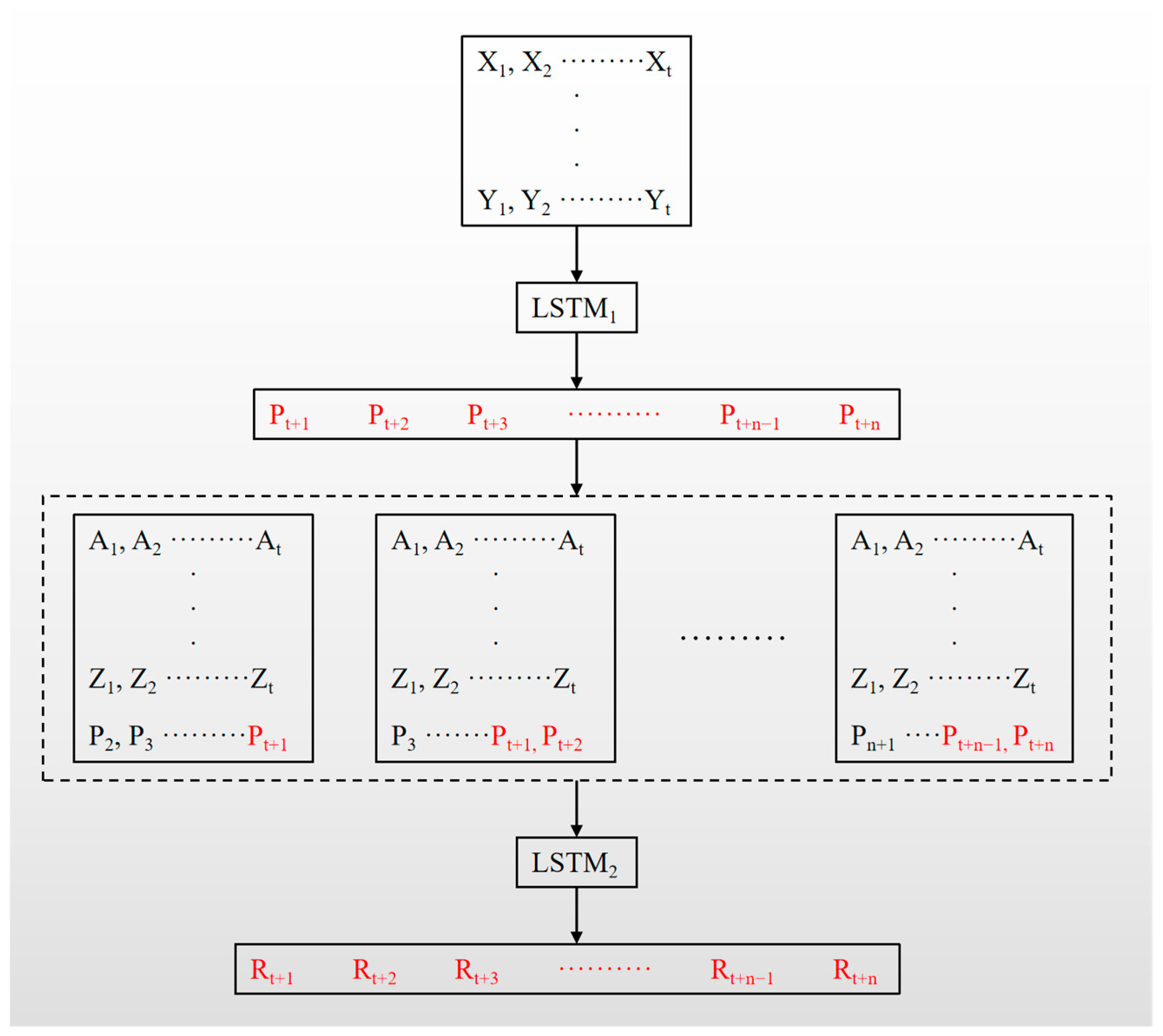
The LSTM method was shown to be effective in time-series forecast, but still has some limitations in streamflow forecast. For example, the target value of the current step t is not only related to the variables of the previous steps (e.g., t − 1, t − 2, …, and t − n), but also to other variables of the current step t. For example, in smaller basins, precipitation rapidly produces river flows to form cross-sectional outlet streamflow, and precipitation at the current step significantly affects streamflow at the current step. This does not mean that precipitation at the current step in large basins is not relevant. When the precipitation center is close to the cross-sectional outlet, it is also possible to quickly form cross-sectional streamflow. In order to solve this problem, this study uses cascade modeling, which is set up to obtain the precipitation at the current step, and also to reduce the complexity of the streamflow forecast layer and improve the generalization capability. The cascade model consists of 2 layers of sub-models, the first layer is the precipitation forecast layer (LSTM_P) and the second layer is the streamflow forecast layer (LSTM_S). LSTM_P is predicting precipitation by using historical observation meteorological variables, and LSTM_ S predicts streamflow by combining historical observation data with the new precipitation data. The new precipitation data is a combination of historical precipitation and precipitation predicted by LSTM_P (Figure 2).
2.4. Experimental Design
The 1979–2017 meteorological forcing data (CN05.1 and CLDAS precipitation and CMFD near-surface air temperature, surface pressure, wind speed, humidity, and the shortwave and longwave radiation fluxes) were interpolated to 6 km resolution and used to drive the CSSPv2 model to obtain synthetic streamflow data at daily and monthly time scales [18]. Then, the Kling–Gupta efficiency (KGE) values were calculated between the monthly simulated streamflow and the observed streamflow for different watersheds in the Yangtze River basin. When the KGE is greater than 0.5, we consider that the model has a relatively good performance in the watershed, and we use the CSSPv2-simulated streamflow as the synthetic streamflow since the observations cannot cover the whole period of 1979–2017 at a daily time scale.
All hydrometeorological data were divided into a training set (1979–2007) and test set (2008–2017). In order to avoid the influence of data scales on the training process, all data were normalized as:
where and are the normalized and the original values, and , are the maximum and minimum values in the training period.
Machine learning settings are as follows:
1. A default LSTM model driven by historical streamflow, precipitation, soil moisture, and evapotranspiration, is used to predict streamflow (STRF), i.e., ([STRF, SM, ET, and P] → STRF). This experiment is used to investigate the capability of LSTM for streamflow simulation without data errors. This experiment is called “default LSTM”.
2. First, we use 850 hpa geopotential height (Geo), surface pressure (Pres), wind speed (V), surface air temperature (T), and surface air specific humidity (Q) from ERA5 to predict future precipitation (LSTM_P), i.e., ([Geo, Pres, V, T, and Q] → Pf). Then, we use historical streamflow, soil moisture, evapotranspiration, and historical precipitation and LSTM_P to predict streamflow (LSTM_S), i.e., ([STRF, SM, ET, and Pf] → STRF), to explore the capability of cascade LSTM model (Figure 2) in streamflow forecast. Note that the above experiments are conducted in the forecasting periods of 1–15 days. This experiment is called “cascade LSTM”.
3. We skip the first step in the “cascade LSTM” experiment, while using observed precipitation instead. Then we repeat the second step in the “cascade LSTM” experiment. This experiment is called “cascade LSTM with perfect precipitation”, which is used to assess the potential (or upper limit) of cascade LSTM.
The study relied on open source libraries, including numpy, math, and panda. Tensorflow was used to implement LSTM and Matplotlib was used to draw the graphs. All experiments were conducted on a server equipped with an AMD EPYC 7402 CPU and an NVIDIA GeForce RTX 3090 GPU. All LSTM models are set up with one hidden layer and one dense layer. The ephemeris is set to 500, the time step is 30 days, the batch size is 256, the hidden cell is 64, the dropout rate is 0.1 and the learning rate is 0.1. The hyper-parameters of the default LSTM model are optimized through grid screening in the one-day lead streamflow forecasts at four stations (zhimenda, cuntan, hankou, and datong) in the mainstream of the Yangtze River, and the hyper-parameters of all subsequent LSTM models remain unchanged (Table 1). The Adam optimizer is chosen as the optimizer and tanh is used as the activation function and given the restriction that its output cannot be less than 0.
2.5. Evaluation of Model Performance
In this study, the Kling–Gupta efficiency (KGE) [39,40] is used to evaluate the forecast results. The KGE is defined as:
where and are the mean values of observed and predicted streamflow during the evaluation period individually, while and are their standard deviations. The R, β, and γ are the Pearson correlation coefficient, the ratio of predicted and observed means (e.g., bias ratio), and the ratio of the predicted and observed coefficient of variation ratio, respectively [41]. The KGE value ranges from negative infinite to one, and a KGE value of one implies a perfect forecast.
3. Results
3.1. Evaluation of CSSPv2 Land Model Simulation and Default LSTM Forecast
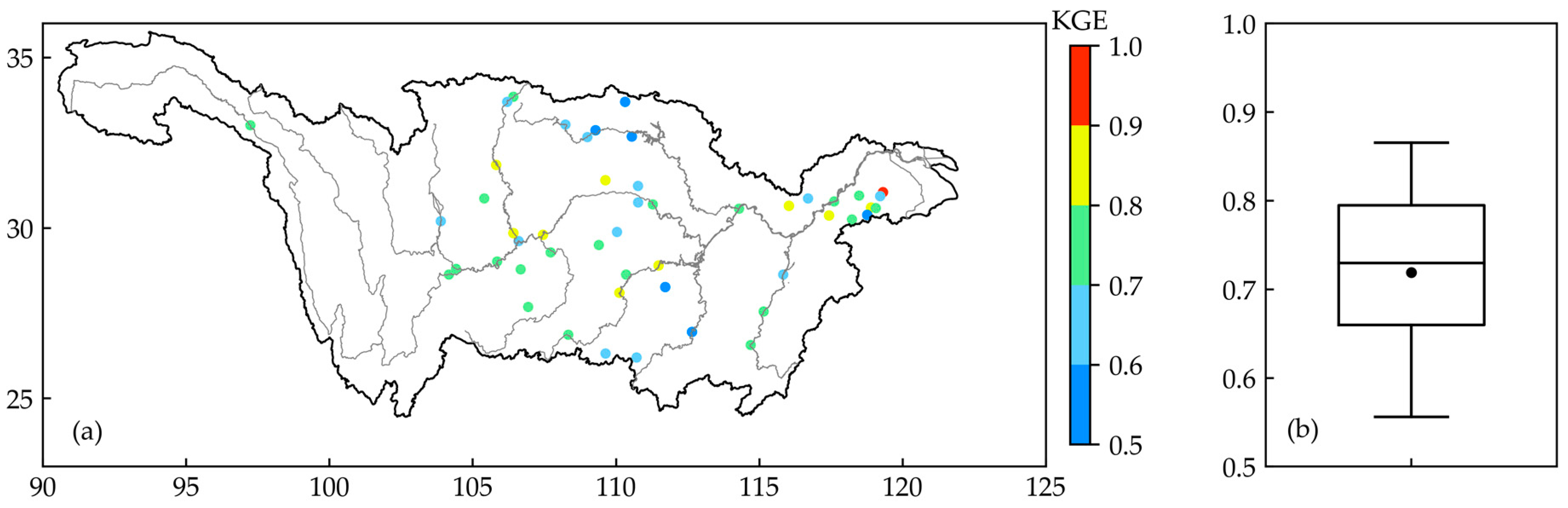
The streamflow simulated by the CSSPv2 land surface model showed good performance (Figure 3a), with the KGE of all stations greater than 0.5 and a median value of 0.72 (Figure 3b) for monthly streamflow. Most of upstream and downstream KGEs are greater than 0.7, except that the KGEs of five tributary stations in the middle reaches of the Yangtze River are between 0.5 and 0.6. Therefore, the synthetic streamflow data (CSSPv2-simulated streamflow data) from all 49 stations are used for the assessments of LSTM modeling.
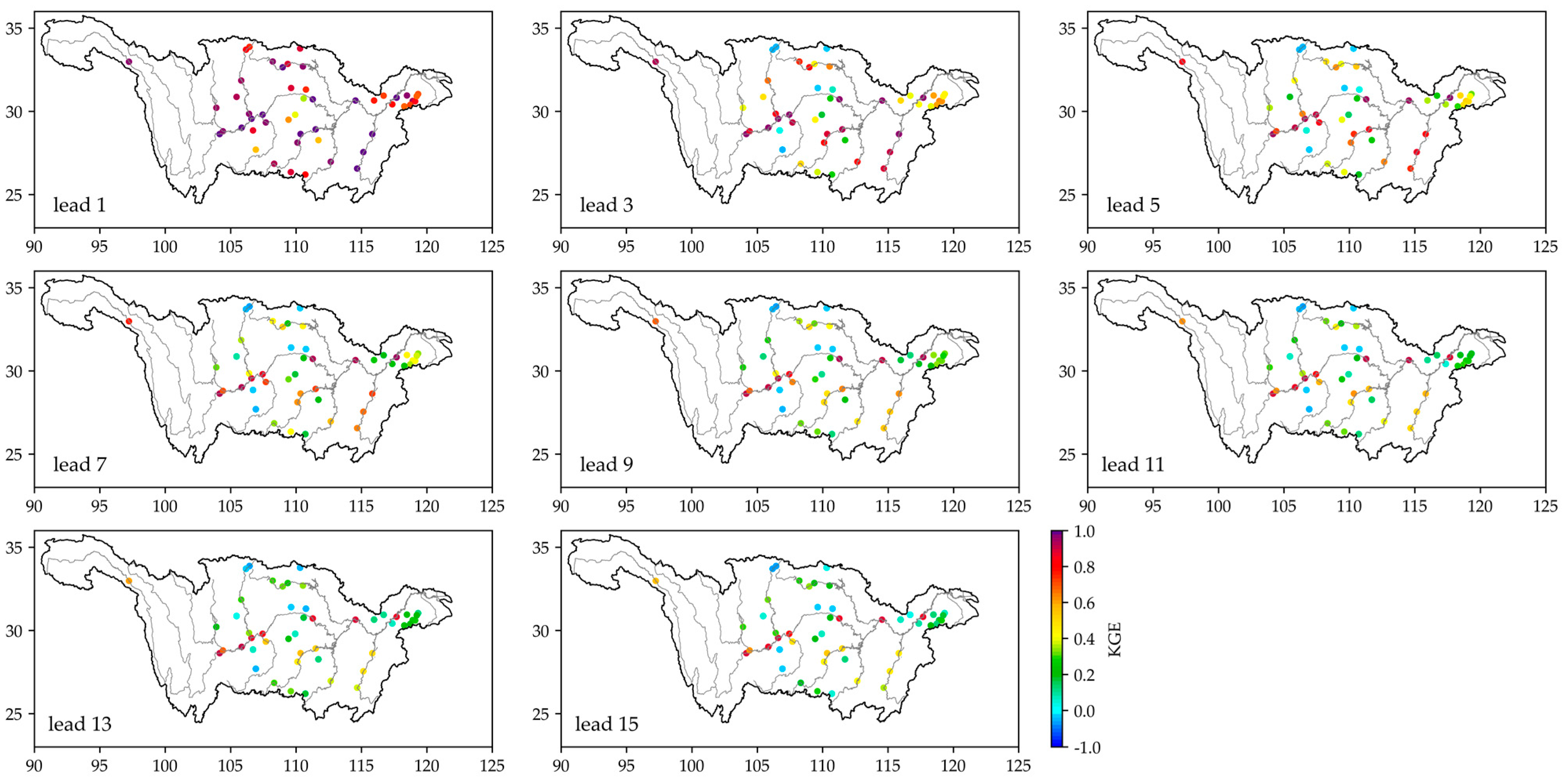
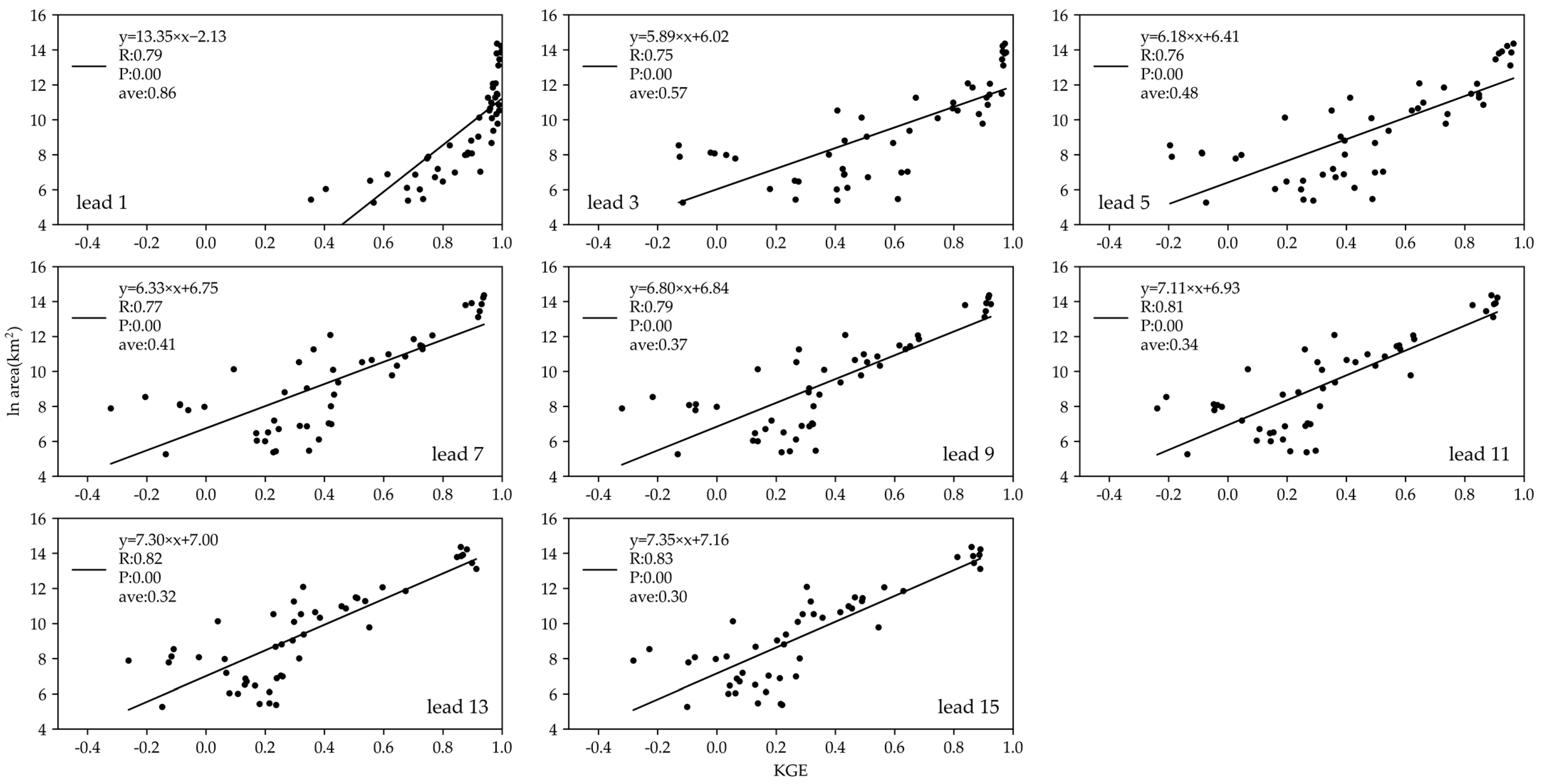
With the synthetic daily streamflow data generated by the CSSPv2 model, the default LSTM models (without predicting precipitation in a cascading manner) are trained and evaluated. Figure 4 shows that 80% of the stations have KGEs greater than 0 at 1–15-day lead times for the default LSTM-predicted daily streamflow. In particular, 78%, 30%, and 20% of the stations have KGEs greater than 0.5 at lead times of 1 day, 7 days, and 15 days, respectively. The mean KGE decreased from 0.86 to 0.41 from a 1-day lead to a 7-day lead, and down to 0.3 at a 15-day lead. As the lead time increases, the forecast skill decreases. Figure 5 shows the larger watershed area, the higher forecast skill is for different lead times. The slower decline of forecast skill of large watersheds may be due to the longer routing time. However, for small watersheds, the skill degradation rate is faster, where the KGEs are 0.3–0.75 at a 1-day lead, while they decrease to −0.35–0.4 at a 7-day lead, and −0.35–0.3 at a 15-day lead times. This may be because the streamflow change of small watersheds is easily affected by rainstorm, and the streamflow response speed is fast. Therefore, real-time or near-real-time precipitation data are critical for streamflow nowcasting and forecasting at small watersheds.
3.2. Evaluation of Cascade LSTM
3.2.1. Precipitation Forecast Based on LSTM_P
Using default LSTM as the baseline, we build cascade LSTM by predicting precipitation firstly. Figure 6 shows the relationship between cascade LSTM-predicted precipitation and watershed area. Similar to the streamflow forecast, the precipitation forecast skill increases as the area increases. About 98%, 53%, and 51% of the stations have KGE greater than 0 for 1, 7, and 15-day lead times. The average KGE for precipitation forecast decreases from 0.27 to 0.07 for 1–15 days lead. Precipitation forecast is very difficult, and there is no skill (KGE < 0) at several small watersheds.
3.2.2. Streamflow Forecast Based on LSTM_S
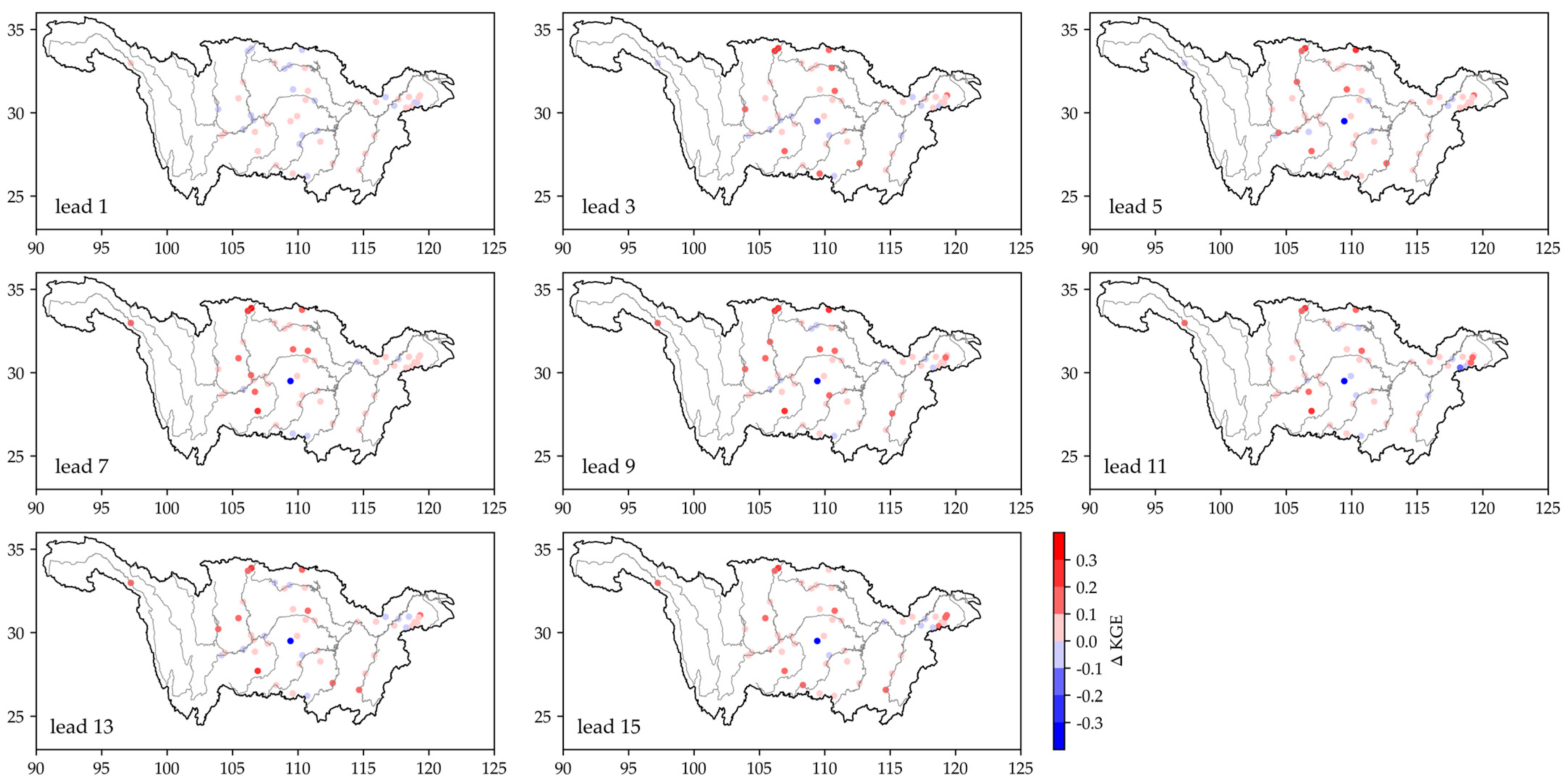
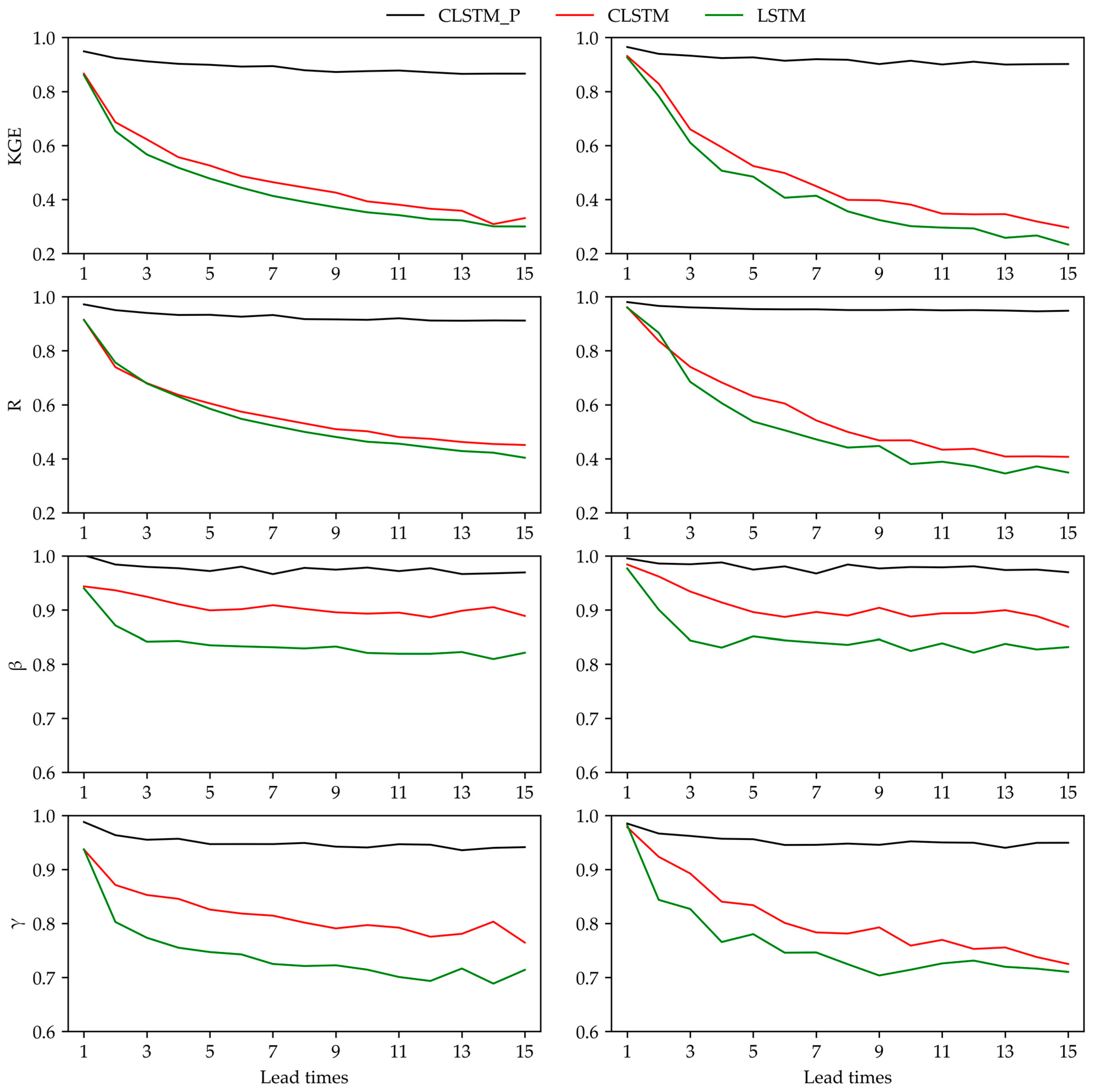
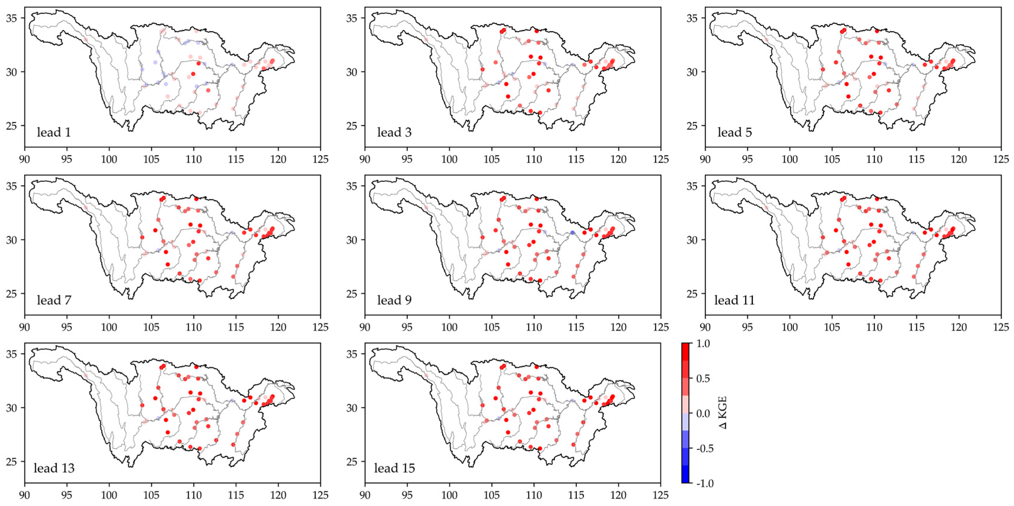
With the predicted precipitation through LSTM_P, cascade LSTM predicts streamflow through LSTM_S (see Section 2.3 for details). Figure 7 shows the KGE difference between cascade LSTM and default LSTM streamflow forecast. From default LSTM to cascade LSTM, 61% of the stations have an increase in KGE, and 75%, 88%, and 88% of the stations have an increase in KGE at 3, 7, and 15 days lead times, where the KGE increases by 0.1–0.3 for 20%, 20%, and 22% of the stations. For the three components of KGE, correlation (R) increases at 53%, 82%, and 84% of the stations at lead times of 1, 7, 15 days, bias in mean value (β) reduces at 57%, 63%, and 63% of the stations, and bias in coefficient of variations (γ) reduces at 59%, 65%, and 43% of the stations. Figure 8 and Table 2 show that the three components from cascade LSTM improved against default LSTM for more than 50% of the stations at most lead times. This suggests that the benefit of cascade LSTM against default LSTM is more obvious at longer lead times.
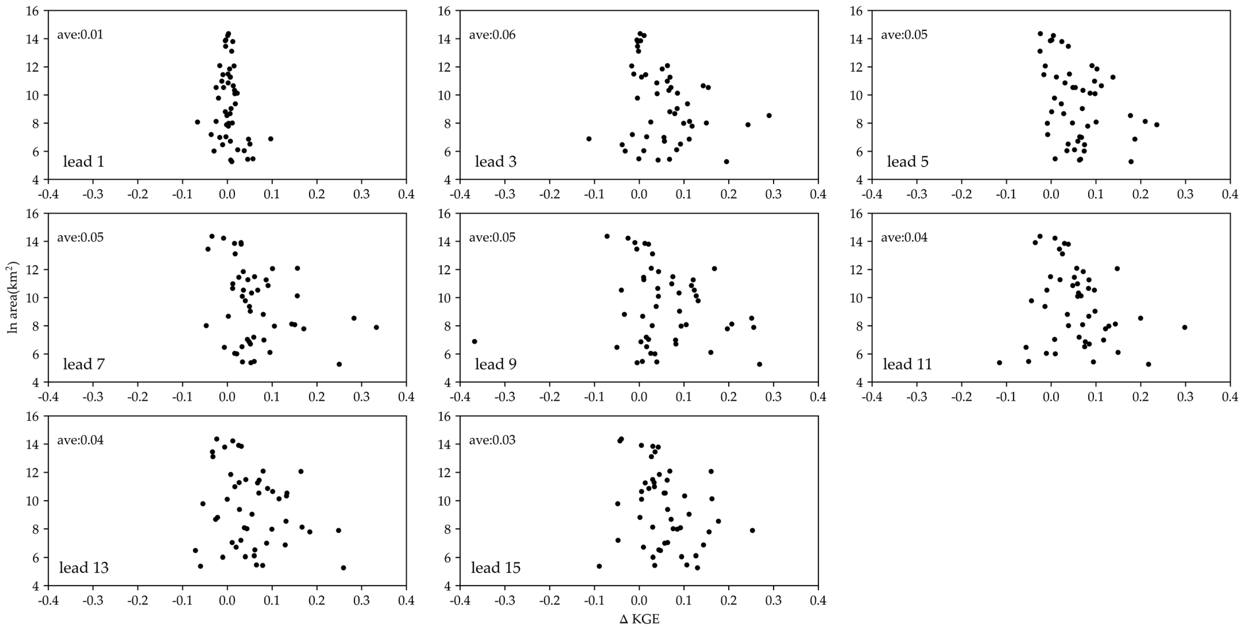
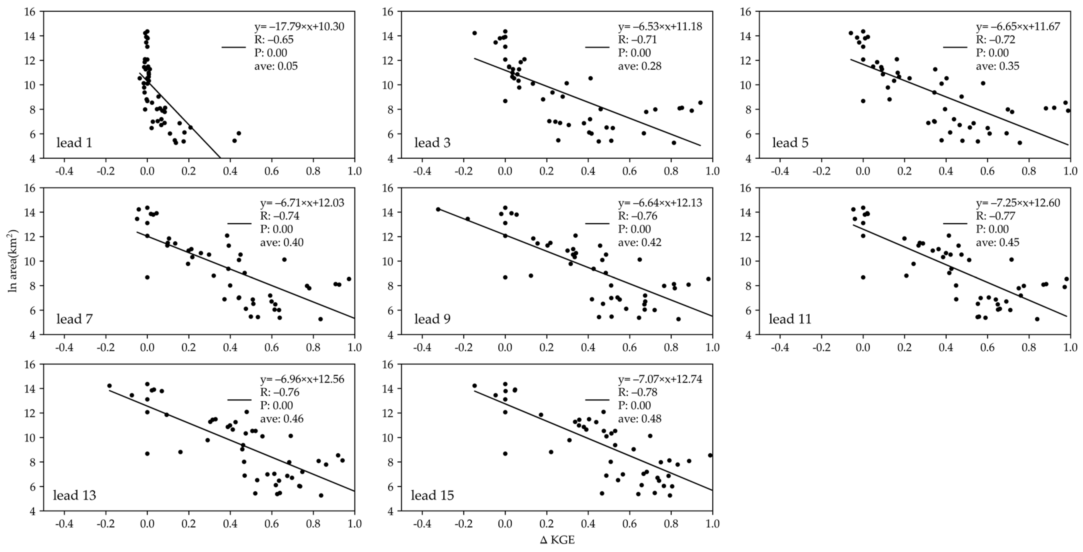
Compared with default LSTM, the average KGE of cascade LSTM streamflow forecast increased by 0.01–0.06 at lead times of 1–15 days (Figure 9). Due to the poor performance of precipitation forecast in small watersheds, the improvement of streamflow forecast is small over these watersheds. For large watersheds, although the precipitation forecast through LSTM_P is good, the LSTM_S does not necessarily have more improvement against default LSTM than those for small watersheds because the rainfall-runoff process does not necessarily dominate the streamflow forecast for large watersheds; other factors including initial memory and river routing might also be important. Therefore, Figure 9 does not show a linear relationship between KGE improvement and basin area. Nevertheless, the improvement of cascade LSTM against default LSTM cannot be ignored for both large and small watersheds over the Yangtze River basin.
3.3. Evaluation of Cascade LSTM with Prefect Precipitation
To explore the potential of cascade LSTM, we conducted a set of ideal experiments, where future precipitation forecasts were replaced with observations, which was called cascade LSTM with perfect precipitation. Figure 10 shows the KGE difference between cascade LSTM with prefect precipitation and default LSTM streamflow forecasts. At 1, 7, and 15-day lead times, KGE increases at 70%, 94%, and 94% of the stations. For the three components of KGE, R increases at 86%, 94%, and 94% of the stations at lead times of 1, 7, and 15 days, β reduces (improves) at 65%, 84%, and 88% of the stations, and γ reduces (improves) at 65%, 88%, and 88% of the stations (Table 2). Figure 8 shows that the cascade LSTM with perfect precipitation is better than the cascade LSTM and the default LSTM both for the mean and median values of the evaluation indicators. With the increase in lead times, the decrease in the correlation coefficient (R) becomes the leading factor for the decrease in KGE. The perfect precipitation experiment shows the importance of precipitation in streamflow forecasts, especially at long leads. When the lead time is greater than 1 day, 25–65% of the stations have KGE increases greater than 0.5. Figure 11 shows that compared with the default LSTM, the cascade LSTM with prefect precipitation has no significant improvement at the 1-day lead time for medium and large watersheds, while the increment of KGE in small watersheds can reach 0.55. For the lead times of 2–15 days, the skill improvement also diminishes as the watershed area increases. This suggests that a perfect precipitation would be more useful for streamflow forecasts at smaller watersheds. On average, the increment of KGE is 0.09–0.48 for the forecasts at 1–15 days.
4. Discussion
Our results have several limitations that need further improvements. Firstly, we used the synthetic data of the physical hydrological model (CSSPv2) to train the LSTM models and carry out the analysis. We focused on the predictions of natural streamflow in both large and small basins, and assumed that the major uncertainty comes from the representations of the rainfall-runoff processes and river routing processes, while we neglected the uncertainties from meteorological forcings and influences of human interventions, such as reservoirs regulations. We are now developing the CSSPv2 model by considering land use/land cover change, reservoir regulations, irrigations, and urbanizations, etc. Combining physical models with LSTM models would show promising prediction capability. Nevertheless, we believe that the current results are useful for understanding the first order processes that control runoff generations, i.e., rainfall-runoff processes [24]. Additionally, we show the potential of precipitation forecasting in the streamflow predictions at different leads.
Secondly, the model of precipitation forecast layer (LSTM_P) can also be modified. Here we only use the LSTM model, while the models applied to precipitation prediction also include machine learning methods that can simulate the characteristics of space-time variations of precipitation, such as the post-processing of radar or weather forecast model data by convolution neural network [42,43] and the direct modeling and prediction of the three-dimensional convolution neural network [44]. The precipitation with spatiotemporal characteristics connected to the LSTM model may be suitable for the predictions of precipitation and runoff in large basins [45]. For example, when the precipitation center is closer to the outlet of a catchment, it can speed up the occurrence of peak flow, which could be considered in the LSTM model.
Thirdly, from the evaluation of the cascade LSTM with perfect precipitation, it is found that precipitation forecasting (even watershed average precipitation) is very important for streamflow forecasting in small watersheds. This study implies the potential of cascade LSTM in the streamflow forecast at small watersheds. More attention should be paid on these small watersheds where the streamflow forecast skill is limited as long leads, especially for deploying more in situ rainfall gauges and radars and developing high-resolution hydro-climate forecast models.
5. Conclusions
In this study, we build cascade LSTM models over 49 watersheds in the Yangtze River basin by using synthetic hydrometeorological data from a high-resolution land surface model simulation, and evaluate streamflow forecast skill at lead times of 1–15 days for default LSTM, cascade LSTM, and cascade LSTM with prefect precipitation.
The results show that the default LSTM model provides skillful streamflow forecast for most watersheds. At the lead times of 1, 7, and 15 days, the KGE of 78%, 30%, and 20% watersheds are greater than 0.5, respectively. Their performance improves as watershed area increases. In addition, the mean KGE decreases from 0.86 to 0.30 during the 1–15-day lead times. The KGE decreases more slowly for larger watersheds. However, the KGE decreases from 0.3–0.75 to −0.35–0.35 for the small watersheds. Large watersheds rely more on historical streamflow data, while small watersheds may rely more on shorter historical data and real-time and near-real-time precipitation data. After implementing the cascade LSTM model, 61–88% of the watersheds show an increase in the KGE at different leads, and the increase at longer leads is more obvious (e.g., 22% of the watersheds show an increase in KGE between 0.1 and 0.3 at 15-day lead times). From default LSTM to cascade LSTM, the average KGE increases by 0.01–0.06 for all watersheds at the 1–7-day lead times. Using a cascade LSTM with perfect precipitation shows further improvements, especially in small watersheds. When the lead times are greater than 1 day, 25–65% of the watersheds have an incremental KGE greater than 0.5. Overall, the cascade LSTM model is a good attempt to forecast streamflow in the Yangtze River basin.
Author Contributions
Conceptualization, J.L. and X.Y.; methodology, J.L. and X.Y.; software, J.L.; writing—original draft preparation, J.L.; writing—review and editing, J.L. and X.Y.; funding acquisition, X.Y. All authors have read and agreed to the published version of the manuscript.
Funding
This work was supported by National Key R&D Program of China (2022YFC3002803), National Natural Science Foundation of China (U22A20556), Natural Science Foundation of Jiangsu Province for Distinguished Young Scholars (BK20211540), Postgraduate Research & Practice Innovation Program of Jiangsu Province (KYCX21_1009), and the Major Science and Technology Program of the Ministry of Water Resources of China (SKS-2022001).
Data Availability Statement
Not applicable.
Conflicts of Interest
The authors declare that they have no known competing financial interest or personal relationships that could have appeared to influence the work reported in this paper.
References
- Arial, P.A.; Bellouin, N.; Coppola, E.; Jones, R.G.; Krinner, G.; Marotzke, J.; Naik, V.; Palmer, M.D.; Plattner, G.-K.; Rogelj, J.; et al. Technical Summary. Climate Change 2021: The Physical Science Basis. Contribution of Working Group I to the Sixth Assessment Report of the Intergovernmental Panel on Climate Change. 2021. Available online: https://www.ipcc.ch/report/ar6/wg1/chapter/technical-summary (accessed on 29 August 2021).
- Behnke, R.; Vavrus, S.; Allstadt, A.; Albright, T.; Thogmartin, W.E.; Radeloff, V.C. Evaluation of downscaled, gridded climate data for the conterminous United States. Ecol. Appl. 2016, 26, 1338–1351. [Google Scholar] [CrossRef] [PubMed]
- Timmermans, B.; Wehner, M.; Cooley, D.; O’Brien, T.; Krishnan, H. An evaluation of the consistency of extremes in gridded precipitation data sets. Clim. Dyn. 2019, 52, 6651–6670. [Google Scholar] [CrossRef] [Green Version]
- Alfieri, L.; Burek, P.; Dutra, E.; Krzeminski, B.; Muraro, D.; Thielen, J.; Pappenberger, F. GloFAS—Global ensemble streamflow forecasting and flood early warning. Hydrol. Earth Syst. Sci. 2013, 17, 1161–1175. [Google Scholar] [CrossRef] [Green Version]
- Coulibaly, P.; Anctil, F.; Rasmussen, P.; Bobée, B. A recurrent neural networks approach using indices of low-frequency climatic variability to forecast regional annual runoff. Hydrol. Process. 2000, 14, 2755–2777. [Google Scholar] [CrossRef]
- Berghuijs, W.; Larsen, J.R.; Van Emmerik, T.H.M.; Woods, R.A. A Global Assessment of Runoff Sensitivity to Changes in Precipitation, Potential Evaporation, and Other Factors. Water Resour. Res. 2017, 53, 8475–8486. [Google Scholar] [CrossRef] [Green Version]
- Yuan, X. An experimental seasonal hydrological forecasting system over the Yellow River basin—Part 2: The added value from climate forecast models. Hydrol. Earth Syst. Sci. 2016, 20, 2453–2466. [Google Scholar] [CrossRef] [Green Version]
- Yuan, X.; Ji, P.; Wang, L.; Liang, X.; Yang, K.; Ye, A.; Su, Z.; Wen, J. High-Resolution Land Surface Modeling of Hydrological Changes Over the Sanjiangyuan Region in the Eastern Tibetan Plateau: 1. Model Development and Evaluation. J. Adv. Model. Earth Syst. 2018, 10, 2806–2828. [Google Scholar] [CrossRef]
- Frame, J.; Kratzert, F.; Raney, A.; Rahman, M.; Salas, F.R.; Nearing, G.S. Post-Processing the National Water Model with Long Short-Term Memory Networks for Streamflow Predictions and Model Diagnostics. J. Am. Water Resour. Assoc. 2021, 57, 885–905. [Google Scholar] [CrossRef]
- Gauch, M.; Mai, J.; Lin, J. The proper care and feeding of CAMELS: How limited training data affects streamflow prediction. Environ. Model. Softw. 2020, 135, 104926. [Google Scholar] [CrossRef]
- Nearing, G.; Pelissier, C.; Kratzert, F.; Klotz, D.; Gupta, H.; Frame, J.; Sampson, A. Physically Informed Machine Learning for Hydrological Modeling Under Climate Nonstationarity. Science and Technology Infusion Climate Bulletin. NOAA’s National Weather Service. In Proceedings of the 44th NOAA Annual Climate Diagnostics and Prediction Workshop, Durham, NC, USA, 22–24 October 2019; Available online: https://www.nws.noaa.gov/ost/climate/STIP/44CDPW/44cdpw-GNearing.pdf (accessed on 26 August 2020). [CrossRef]
- Hoedt, P.; Kratzert, F.; Klotz, D.; Halmich, C.; Holzleitner, M.; Nearing, G.; Hochreiter, S.; Klambauer, G. MC-LSTM: Mass-Conserving LSTM. arXiv 2021, arXiv:2101.05186. [Google Scholar] [CrossRef]
- Liu, J.; Yuan, X.; Zeng, J.; Jiao, Y.; Li, Y.; Zhong, L.; Yao, L. Ensemble streamflow forecasting over a cascade reservoir catchment with integrated hydrometeorological modeling and machine learning. Hydrol. Earth Syst. Sci. 2022, 26, 265–278. [Google Scholar] [CrossRef]
- Kratzert, F.; Klotz, D.; Brenner, C.; Schulz, K.; Herrnegger, M. Rainfall–runoff modelling using Long Short-Term Memory (LSTM) networks. Hydrol. Earth Syst. Sci. 2018, 22, 6005–6022. [Google Scholar] [CrossRef] [Green Version]
- Kratzert, F.; Klotz, D.; Herrnegger, M.; Sampson, A.K.; Hochreiter, S.; Nearing, G.S. Toward Improved Predictions in Ungauged Basins: Exploiting the Power of Machine Learning. Water Resour. Res. 2019, 55, 11344–11354. [Google Scholar] [CrossRef] [Green Version]
- Rahimzad, M.; Moghaddam, N.; Alireza, Z.; Hosam, S.; Jaber, D.; Mehr, A.; Kwon, H. Performance Comparison of an LSTM-based Deep Learning Model versus Conventional Machine Learning Algorithms for Streamflow Forecasting. Water Resour. Manag. 2021, 35, 4167–4187. [Google Scholar] [CrossRef]
- Cheng, M.; Fang, F.; Kinouchi, T.; Navon, I.; Pain, C. Long lead-time daily and monthly streamflow forecasting using machine learning methods. J. Hydrol. 2020, 590, 125376. [Google Scholar] [CrossRef]
- Zhu, S.; Luo, X.; Yuan, X.; Xu, Z. An improved long short-term memory network for streamflow forecasting in the upper Yangtze River. Stoch. Environ. Res. Risk Assess. 2020, 34, 1313–1329. [Google Scholar] [CrossRef]
- Cho, K.; Kim, Y. Improving streamflow prediction in the WRF-Hydro model with LSTM networks. J. Hydrol. 2022, 605, 127297. [Google Scholar] [CrossRef]
- Hu, X.; Chu, L.; Pei, J.; Liu, W.; Bian, J. Model complexity of deep learning: A survey. Knowl. Inf. Syst. 2021, 63, 2585–2619. [Google Scholar] [CrossRef]
- Feng, D.; Fang, K.; Shen, C. Enhancing Streamflow Forecast and Extracting Insights Using Long-Short Term Memory Networks With Data Integration at Continental Scales. Water Resour. Res. 2020, 56, e2019WR026793. [Google Scholar] [CrossRef]
- Jain, S.; Mani, S.; Jain, S.K.; Prakash, P.; Singh, V.P.; Tullos, D.; Kumar, S.; Agarwal, S.P.; Dimri, A.P. A brief review of flood forecasting techniques and their applications. Int. J. River Basin Manag. 2018, 16, 329–344. [Google Scholar] [CrossRef]
- Granata, F.; Di Nunno, F.; de Marinis, G. Stacked machine learning algorithms and bidirectional long short-term memory networks for multi-step ahead streamflow forecasting: A comparative study. J. Hydrol. 2022, 613, 128431. [Google Scholar] [CrossRef]
- Bai, Y.; Bezak, N.; Sapač, K.; Klun, M.; Zhang, J. Short-Term Streamflow Forecasting Using the Feature-Enhanced Regression Model. Water Resour. Manag. 2019, 33, 4783–4797. [Google Scholar] [CrossRef]
- Ji, P.; Yuan, X.; Shi, C.; Jiang, L.; Wang, G.; Yang, K. A Long-Term Simulation of Land Surface Conditions at High Resolution over Continental China. J. Hydrometeorol. 2023, 24, 285–314. [Google Scholar] [CrossRef]
- Shangguan, W.; Dai, Y.; Duan, Q.; Liu, B.; Yuan, H. A global soil data set for earth system modeling. J. Adv. Model. Earth Syst. 2014, 6, 249–263. [Google Scholar] [CrossRef]
- Liang, S.; Cheng, J.; Jia, K.; Jiang, B.; Liu, Q.; Xiao, Z.; Yao, Y.; Yuan, W.; Zhang, X.; Zhao, X.; et al. The Global Land Surface Satellite (GLASS) Product Suite. Bull. Am. Meteorol. Soc. 2021, 102, E323–E337. [Google Scholar] [CrossRef]
- Yuan, X.; Liang, X.-Z. Evaluation of a Conjunctive Surface–Subsurface Process Model (CSSP) over the Contiguous United States at Regional–Local Scales. J. Hydrometeorol. 2011, 12, 579–599. [Google Scholar] [CrossRef]
- Hersbach, H.; Bell, B.; Berrisford, P.; Hirahara, S.; Horanyi, A.; Muñoz-Sabater, J.; Nicolas, J.; Peubey, C.; Radu, R.; Schepers, D.; et al. The ERA5 global reanalysis. Q. J. R. Meteorol. Soc. 2020, 146, 1999–2049. [Google Scholar] [CrossRef]
- Dai, Y.; Dickinson, R.; Wang, Y. A two-big-leaf model for canopy temperature, photosynthesis, and stomatal conductance. J. Clim. 2004, 17, 2281–2299. [Google Scholar] [CrossRef]
- Choi, H.; Kumar, P.; Liang, X.-Z. Three-dimensional volume-averaged soil moisture transport model with a scalable parameterization of subgrid topographic variability. Water Resour. Res. 2007, 43, W04414. [Google Scholar] [CrossRef] [Green Version]
- Choi, H.; Liang, X.-Z.; Kumar, P. A Conjunctive Surface–Subsurface Flow Representation for Mesoscale Land Surface Models. J. Hydrometeorol. 2013, 14, 1421–1442. [Google Scholar] [CrossRef]
- Liang, X.; Lettenmaier, D.P.; Wood, E.F.; Burges, S.J. A simple hydrologically based model of land surface water and energy fluxes for general circulation models. J. Geophys. Res. Atmos. 1994, 99, 14415–14428. [Google Scholar] [CrossRef]
- Liang, X.Z.; Xu, M.; Yuan, X.; Ling, T.; Choi, H.I.; Zhang, F.; Chen, L.; Liu, S.; Su, S.; Qiao, F.; et al. Regional Climate–Weather Research and Forecasting Model. Bull. Am. Meteorol. Soc. 2012, 93, 1363–1387. [Google Scholar] [CrossRef]
- Ji, P.; Yuan, X.; Liang, X.-Z. Do Lateral Flows Matter for the Hyperresolution Land Surface Modeling? J. Geophys. Res. Atmos. 2017, 122, 12077–12092. [Google Scholar] [CrossRef] [Green Version]
- Zheng, D.; Van Der Velde, R.; Su, Z.; Wen, J.; Wang, X. Assessment of Noah land surface model with various runoff parameterizations over a Tibetan river. J. Geophys. Res. Atmos. 2017, 122, 1488–1504. [Google Scholar] [CrossRef]
- Ji, P.; Yuan, X.; Jiao, Y.; Wang, C.; Han, S.; Shi, C. Anthropogenic Contributions to the 2018 Extreme Flooding over the Upper Yellow River Basin in China. Bull. Am. Meteorol. Soc. 2020, 101, S89–S94. [Google Scholar] [CrossRef] [Green Version]
- Zeng, J.; Yuan, X.; Ji, P.; Shi, C. Effects of meteorological forcings and land surface model on soil moisture simulation over China. J. Hydrol. 2021, 603, 126978. [Google Scholar] [CrossRef]
- Gupta, H.; Kling, H.; Yilmaz, K.K.; Martinez, G.F. Decomposition of the mean squared error and NSE performance criteria: Implications for improving hydrological modelling. J. Hydrol. 2009, 377, 80–91. [Google Scholar] [CrossRef] [Green Version]
- Kling, H.; Fuchs, M.; Paulin, M. Runoff conditions in the upper Danube basin under an ensemble of climate change scenarios. J. Hydrol. 2012, 424–425, 264–277. [Google Scholar] [CrossRef]
- Chen, Y.; Yuan, H. Evaluation of nine sub-daily soil moisture model products over China using high-resolution in situ observations. J. Hydrol. 2020, 588, 125054. [Google Scholar] [CrossRef]
- Zhang, C.; Brodeur, Z.P.; Steinschneider, S.; Herman, J.D. Leveraging Spatial Patterns in Precipitation Forecasts Using Deep Learning to Support Regional Water Management. Water Resour. Res. 2022, 58, e2021WR031910. [Google Scholar] [CrossRef]
- Sha, Y.; Ii, D.J.G.; West, G.; Stull, R. A hybrid analog-ensemble, convolutional-neural-network method for post-processing precipitation forecasts. Mon. Weather. Rev. 2022, 1, 1495–1515. [Google Scholar] [CrossRef]
- Chen, G.; Wang, W. Short-Term Precipitation Prediction for Contiguous United States Using Deep Learning. Geophys. Res. Lett. 2022, 49, e2022GL097904. [Google Scholar] [CrossRef]
- Deng, H.; Chen, W.; Huang, G. Deep insight into daily runoff forecasting based on a CNN-LSTM model. Nat. Hazards 2022, 133, 1675–1696. [Google Scholar] [CrossRef]
Figure 1.
Locations and drainage areas (km2) of 49 streamflow observational stations over the Yangtze River basin in southern China.
Figure 1.
Locations and drainage areas (km2) of 49 streamflow observational stations over the Yangtze River basin in southern China.

Figure 2.
The setting of the cascade LSTM model.

Figure 3.
(a) Spatial distribution of KGE between observed and CSSPv2 model-simulated monthly streamflow over the Yangtze River basin. (b) The boxplot of KGE for all 49 stations. The boxes represent the 25th and 75th percentiles of KGE, the line and the dot within the box are median and mean values of KGE, respectively, and the whiskers represent 10th and 90th percentiles of KGE.

Figure 4.
Spatial distributions of KGEs for streamflow forecasts based on default LSTM model at lead times of 1–15 days.
Figure 4.
Spatial distributions of KGEs for streamflow forecasts based on default LSTM model at lead times of 1–15 days.

Figure 5.
The relationship between the watershed area (ln km2) and the default LSTM streamflow forecast skill (KGE) at the lead times of 1–15 days.
Figure 5.
The relationship between the watershed area (ln km2) and the default LSTM streamflow forecast skill (KGE) at the lead times of 1–15 days.

Figure 6.
The relationship between the watershed area (ln km2) and the LSTM_P precipitation forecast skill (KGE) at the lead times of 1–15 days.
Figure 6.
The relationship between the watershed area (ln km2) and the LSTM_P precipitation forecast skill (KGE) at the lead times of 1–15 days.

Figure 7.
Spatial distributions of the KGE difference (∆ KGE) between the daily streamflow forecasts by the cascade LSTM model and those by the default LSTM model.
Figure 7.
Spatial distributions of the KGE difference (∆ KGE) between the daily streamflow forecasts by the cascade LSTM model and those by the default LSTM model.

Figure 8.
Performance of streamflow forecasts at different lead times. The left column shows the mean values of KGE, R, β, and γ for 49 stations, and the right column shows their median values.
Figure 8.
Performance of streamflow forecasts at different lead times. The left column shows the mean values of KGE, R, β, and γ for 49 stations, and the right column shows their median values.

Figure 9.
The relationship between the difference of streamflow forecast performance (∆ KGE of the cascade LSTM model and the default LSTM model) and the watershed area (ln km2) at the lead times of 1–15 days.
Figure 9.
The relationship between the difference of streamflow forecast performance (∆ KGE of the cascade LSTM model and the default LSTM model) and the watershed area (ln km2) at the lead times of 1–15 days.

Figure 10.
Spatial distributions of the KGE difference (∆ KGE) between the daily streamflow forecasts by the cascade LSTM with prefect precipitation and those by default LSTM.
Figure 10.
Spatial distributions of the KGE difference (∆ KGE) between the daily streamflow forecasts by the cascade LSTM with prefect precipitation and those by default LSTM.

Figure 11.
The relationship between the difference of streamflow forecast performance (∆ KGE of the cascade LSTM model with prefect precipitation and the default LSTM model ) and the watershed area (ln km2) at the lead times of 1–15 days.
Figure 11.
The relationship between the difference of streamflow forecast performance (∆ KGE of the cascade LSTM model with prefect precipitation and the default LSTM model ) and the watershed area (ln km2) at the lead times of 1–15 days.


Table 1.
Hyper-parameter setting of mesh optimization.
| Hyper-Parameter | Set Up |
|---|---|
| Batch | 16, 32, 64, 128, 256, 512, 1024 |
| Hidden cell | 8, 16, 32, 64, 128, 256 |
| Dropout rate | 0.01, 0.05, 0.1, 0.15, 0.2, 0.3 |
| Learning rate | 0.001, 0.005, 0.01, 0.05, 0.1, 0.2 |
Table 2.
Percentage (%) of stations that improved compared to the default LSTM model, the cascaded LSTM model (CLSTM), and the cascaded LSTM with the perfect precipitation (CLSTM_P) model KGE and its three components (R, β and γ).
Table 2.
Percentage (%) of stations that improved compared to the default LSTM model, the cascaded LSTM model (CLSTM), and the cascaded LSTM with the perfect precipitation (CLSTM_P) model KGE and its three components (R, β and γ).
| Lead Times | KGE | R | β | γ | ||||
|---|---|---|---|---|---|---|---|---|
| CLSTM | CLSTM_P | CLSTM | CLSTM_P | CLSTM | CLSTM_P | CLSTM | CLSTM_P | |
| 1 | 0.61 | 0.70 | 0.53 | 0.86 | 0.57 | 0.65 | 0.59 | 0.65 |
| 2 | 0.76 | 0.86 | 0.20 | 0.82 | 0.82 | 0.86 | 0.80 | 0.78 |
| 3 | 0.76 | 0.88 | 0.45 | 0.88 | 0.84 | 0.92 | 0.76 | 0.84 |
| 4 | 0.86 | 0.88 | 0.53 | 0.90 | 0.80 | 0.88 | 0.69 | 0.80 |
| 5 | 0.84 | 0.88 | 0.63 | 0.92 | 0.73 | 0.78 | 0.71 | 0.86 |
| 6 | 0.86 | 0.90 | 0.69 | 0.90 | 0.67 | 0.88 | 0.65 | 0.88 |
| 7 | 0.88 | 0.94 | 0.82 | 0.94 | 0.63 | 0.84 | 0.65 | 0.88 |
| 8 | 0.86 | 0.92 | 0.82 | 0.96 | 0.61 | 0.86 | 0.59 | 0.90 |
| 9 | 0.82 | 0.92 | 0.82 | 0.94 | 0.61 | 0.86 | 0.65 | 0.86 |
| 10 | 0.80 | 0.92 | 0.86 | 0.94 | 0.51 | 0.86 | 0.63 | 0.86 |
| 11 | 0.78 | 0.94 | 0.73 | 0.96 | 0.71 | 0.94 | 0.67 | 0.88 |
| 12 | 0.76 | 0.90 | 0.78 | 0.94 | 0.51 | 0.86 | 0.55 | 0.90 |
| 13 | 0.76 | 0.90 | 0.80 | 0.96 | 0.61 | 0.84 | 0.51 | 0.92 |
| 14 | 0.84 | 0.92 | 0.80 | 0.96 | 0.59 | 0.86 | 0.59 | 0.94 |
| 15 | 0.88 | 0.94 | 0.84 | 0.94 | 0.63 | 0.88 | 0.43 | 0.88 |
Disclaimer/Publisher’s Note: The statements, opinions and data contained in all publications are solely those of the individual author(s) and contributor(s) and not of MDPI and/or the editor(s). MDPI and/or the editor(s) disclaim responsibility for any injury to people or property resulting from any ideas, methods, instructions or products referred to in the content. |
© 2023 by the authors. Licensee MDPI, Basel, Switzerland. This article is an open access article distributed under the terms and conditions of the Creative Commons Attribution (CC BY) license (https://creativecommons.org/licenses/by/4.0/).
Share and Cite
MDPI and ACS Style
Li, J.; Yuan, X. Daily Streamflow Forecasts Based on Cascade Long Short-Term Memory (LSTM) Model over the Yangtze River Basin. Water 2023, 15, 1019. https://doi.org/10.3390/w15061019
AMA Style
Li J, Yuan X. Daily Streamflow Forecasts Based on Cascade Long Short-Term Memory (LSTM) Model over the Yangtze River Basin. Water. 2023; 15(6):1019. https://doi.org/10.3390/w15061019
Chicago/Turabian StyleLi, Jiayuan, and Xing Yuan. 2023. "Daily Streamflow Forecasts Based on Cascade Long Short-Term Memory (LSTM) Model over the Yangtze River Basin" Water 15, no. 6: 1019. https://doi.org/10.3390/w15061019
Note that from the first issue of 2016, this journal uses article numbers instead of page numbers. See further details here.