Article

Increasing Trends in Discharge Maxima of a Mediterranean River during Early Autumn

by
George Varlas
1,*,
Christina Papadaki
1,
Konstantinos Stefanidis
1,
Angeliki Mentzafou
1,
Ilias Pechlivanidis
2,
Anastasios Papadopoulos
1 and
Elias Dimitriou
1
1
Hellenic Centre for Marine Research, Institute of Marine Biological Resources and Inland Waters, 46.7 km of Athens-Sounio Ave., 19013 Anavyssos, Greece
2
Hydrology R&D, Swedish Meteorological and Hydrological Institute, SE-60176 Norrköping, Sweden
*
Author to whom correspondence should be addressed.
Water 2023, 15(6), 1022; https://doi.org/10.3390/w15061022
Submission received: 6 February 2023 / Revised: 1 March 2023 / Accepted: 6 March 2023 / Published: 8 March 2023
(This article belongs to the Special Issue Impacts of Climate Change on Hydrology and Water Resources)

Abstract

:
Climate change has influenced the discharge regime of rivers during the past decades. This study aims to reveal climate-induced interannual trends of average annual discharge and discharge maxima in a Mediterranean river from 1981 to 2017. To this aim, the Pinios river basin was selected as the study area because it is one of the most productive agricultural areas of Greece. Due to a lack of sufficient measurements, simulated daily discharges for three upstream sub-basins were used. The discharge trend analysis was based on a multi-faceted approach using Mann-Kendall tests, Quantile-Kendall plots, and generalized additive models (GAMs) for fitting non-linear interannual trends. The methodological approach proposed can be applied anywhere to investigate climate change effects. The results indicated that the average annual discharge in the three upstream sub-basins decreased in the 1980s, reaching a minimum in the early 1990s, and then increased from the middle 1990s to 2017, reaching approximately the discharge levels of the early 1980s. A more in-depth analysis unraveled that the discharge maxima in September were characterized by statistically significant increasing interannual trends for two of the three sub-basins. These two sub-basins are anthropogenically low affected, thus highlighting the clear impact of climate change that may have critical socioeconomic implications in the Pinios basin.

1. Introduction

Anthropogenic climate change has influenced mean and extreme river flow [1], while it has increased flood risk [2], thus having severe implications worldwide. The Mediterranean region has been characterized as a climate change “hot spot” [3] because its climate is especially responsive to global changes. Climate change has strong effects on temperature, precipitation, and other parameters which determine the local climate. The climatic effects are very intense and complex in the Mediterranean countries such as Greece, characterized by large variabilities in the landscape, orography, and land use [4,5,6]. According to the Sixth Assessment Report of the Intergovernmental Panel on Climate Change (IPCC) published in 2021 [7], the average precipitation over land on a global scale has likely increased since 1950. However, the Mediterranean region seems to suffer from an increase in droughts. A previous study corroborates this finding as it concluded that the annual discharge volume of rivers in the Mediterranean region had presented declining trends for a period from 1950 to 2013 [8]. Moreover, another study showed declining trends of flooding in the Mediterranean region from 1960 to 2010 [9]. Furthermore, climate change influences the alternation of seasons by increasing the disparity between wet and dry ones [10,11,12]. This is another factor that may impact water availability and river discharge. It is noteworthy that several studies have shown that the water resources will probably continue the decreasing trend in the future, causing amplification of droughts and aridity [13,14,15,16].
In Greece, the most recent significant dry period characterized by decreased precipitation and, thus, increased drought in several areas lasted from the late 1980s to the early 1990s [4,17,18,19]. The drought during this period influenced not only Greece but also other Mediterranean countries [20,21,22], having severe implications for the whole Mediterranean region with an economic cost that was estimated to exceed 2.1 billion Euros [23]. Pinios river, which is one of the most productive agricultural areas of Greece and located in central-northern Greece, also suffered from this severe drought which lasted from 1988 to 1993 in this area. It is important to note that especially the drought during 1989–1990 was characterized by an average return period of 88 years for the Pinios river basin [24]. Despite the fact that studies focusing on various Greek rivers [25] and Pinios river [26] have reported climatic variabilities of discharge and drought periods, they did not show significant linear trends during the past decades, at least until 2002 [26] and 2010 [25].
Except for the increasing drought, one of the most significant issues regarding climate change is the change in precipitation extremes [7,27], that under favorable conditions, may trigger catastrophic flash floods in Mediterranean countries [28,29,30,31,32]. There are studies that report the intensification of short-term precipitation extremes induced by anthropogenic climate impacts [33]. Greece has been affected by several extreme precipitation events and floods during the last decades, affecting Thessaly and Pinios river, among other regions, especially during autumn [34,35,36]. It is noteworthy that the number of flood occurrences in Pinios river presented a rising trend during the period 1990–2010 [36]. Precipitation extremes during autumn in Greece have sometimes been related to Mediterranean tropical-like cyclones (“medicanes”), although they are generally rare phenomena, with approximately three medicanes in the whole Mediterranean per 2 years [37]. For example, Numa medicane in November 2017 had indirect effects on the flash flood of Mandra town, causing 24 fatalities [29,30,32]. Zorbas medicane in September 2018 brought torrential rainfall, causing three deaths and severe damage in several Greek areas [38]. Ianos medicane in September 2020 was the most intense medicane ever recorded in the Mediterranean, causing four fatalities and extensive damage in many regions, including Karditsa city and Mouzaki town located in the southwestern parts of the Pinios river basin [35]. An overall assessment of the flash flood in Karditsa city showed that the exceedance probability of the Ianos-induced flood ranged from 1:400 years in the low-lying catchments to 1:1000 years in the upstream mountainous catchments.
Therefore, there is the assumption that discharge maxima in Pinios river have increased during the last decades, especially in autumn. These maxima sometimes imply severe hydrometeorological phenomena and floods associated with high socioeconomic impacts. Multi-year analyses, also including a period after 2010 that is critical in terms of climate change effects, are needed to reveal significant trends in discharge maxima if they exist. However, Pinios river has not been covered by sufficient monitoring during the last decades, thus making long-term studies difficult and uncertain. The Institute of Marine Biological Resources and Inland Waters (IMBRIW) of the Hellenic Centre for Marine Research (HCMR) has developed a monitoring network in the river basin during the last few years, but this cannot facilitate long-term studies yet. The lack of sufficient measurements poses the necessity of alternative research efforts exploiting other sources of data. In this context, modeled discharge data from one of the most reliable and famous hydrological models, namely E-HYPE, were used in this study due to the lack of continuous, long-term, and reliable discharge measurements during the last decades.
In this framework, the scope of this study is to address two scientific questions, using the Pinios river basin as the study area and employing the E-HYPE discharges. The first scientific question is how climate change has influenced monthly discharge maxima over the years? The second one is what is the amplitude of interannual variabilities of average annual discharge? The trend analysis was performed using Mann-Kendall tests, Quantile-Kendall plots, and generalized additive models (GAMs) for fitting non-linear interannual trends. It is important to note here that the methodological approach adopted in this study may have a wider application in other areas and scales. Moreover, this basin is influenced by both climate variabilities and multiple anthropogenic pressures. Hence, we considered two upstream and partially mountainous sub-basins of Pinios to exclude the potential effects of direct anthropogenic pressures and one similar sub-basin that, however, is partially covered by some agricultural areas to investigate possible trend sensitivity by comparing with the two other sub-basins.
The article is structured as follows: Section 2 presents the study area and data used and also described the methodology used to analyze the data. Section 3 presents the results from addressing the scientific questions and objectives. Section 4 presents the discussion, and finally, Section 5 concludes the work.

2. Materials and Methods
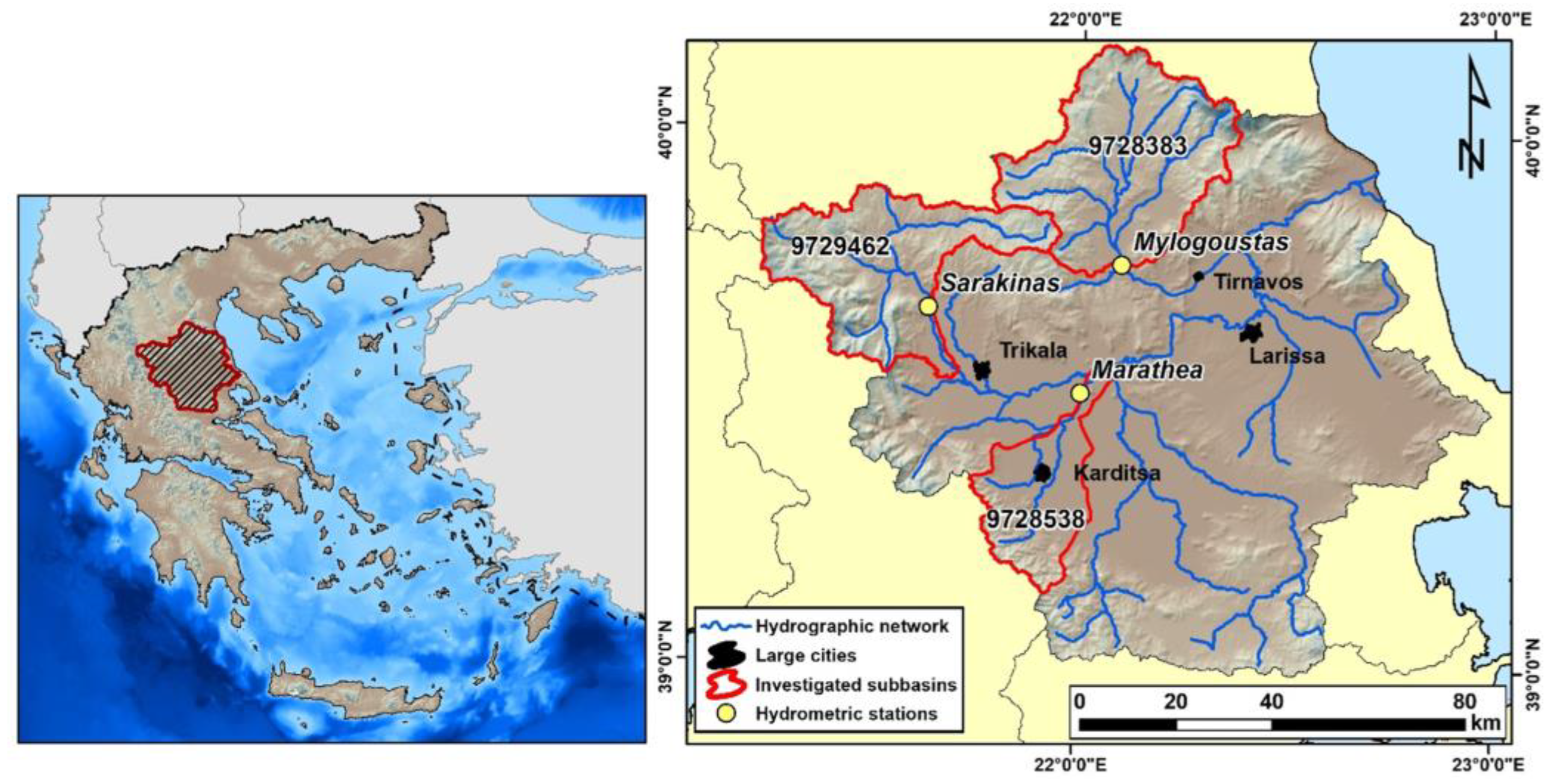
2.1. Study Area

Pinios river basin is located in the administrative region of Thessaly in central-northern Greece. The most populated cities in the area are Larissa, Karditsa, Trikala, and Tirnavos. Pinios was selected because it is one of the most productive areas of Greece, mainly regarding the agricultural sector. The total area of the basin is about 11,000 km2 and is mainly occupied by agricultural land (51% of the total basin area) and secondarily by vegetated areas (45%) [39]. It is noteworthy that the agricultural sector of the Pinios river basin represents 14% of the gross value added of the agricultural industry of Greece [40]. Pinios basin can be subdivided into two separate endorheic hydrographic networks, in the western (Karditsa plain) and the eastern (Larisa plain) basins, respectively, separated by an internal low-lying hill area [41,42]. The hydrographic network of the Pinios basin is complex and can be characterized as dendritic [32]. The climate of the Pinios basin in the western part is typical Mediterranean, with cold winters and moderate precipitation rate, followed by relatively hot and dry summers, while the eastern and northern parts of the basin have a cold semi-arid climate, with warm to hot, dry summers and cold winters [43]. The average annual precipitation at the Pinios basin is about 700 mm, with large spatial variabilities [4], ranging from 450 mm in the central area to 1850 mm in the western-mountainous part of the basin [44].
Pinios is affected by both interannual climate variabilities and multiple anthropogenic pressures [45], including irrigation processes, bridges, technical works, industries, buildings, pollution, etc. Therefore, in the context of this study, we selected three partially mountainous sub-basins upstream of the river to study the net effects of climate change on discharge for the 37-year period. In this way, we reduced the direct anthropogenic effects in our analysis, which are intense mainly in the lowland areas of the basin and could have variable effects on our results for each year of the 37-year period, thus hiding climatic effects. Two of the investigated sub-basins are located in the western part of the Pinios basin and one in the eastern one. More specifically, the 9729462 (Pinios upstream) sub-basin is located at the north-western part of Karditsa plain, the 9728383 (Titarisios tributary) sub-basin is located at the northern part of the Larisa plain, and the 9728538 (Mega Rema tributary) sub-basin is located at the southwestern part of Karditsa plain (Figure 1). The names of the sub-basins (i.e., 9729462, 9728383, and 9728538) used in this study were based on the encoding used in the European Hydrological Predictions for the Environment (E-HYPE) model data. E-HYPE data were used in this study and are described in the next subsection. In particular, the names 9729462, 9728383, and 9728538 refer to the outflow sub-basins as defined in the E-HYPE model data, but we considered these names for the entire sub-basins under study. For the convenience of readers, the 9729462, 9728383, and 9728538 sub-basins are referred to in the text, also using the code names PINUP, TITAR, and MREMA, respectively. The main characteristics of the three sub-basins, including area, surface waterbody, altitude [46], and land cover [39], are shown in Table 1. It is worthwhile noting that the MREMA sub-basin was selected to slightly differ from the other two sub-basins having similarities with low-lying areas of Pinios to explore probable implying effects induced by its lower altitude and increased agriculture (Table 1).

2.2. European Hydrological Predictions for the Environment (E-HYPE) Model Data

For the purpose of the present study, we employed time series of daily discharge values for a 37-year period from 1 January 1981 to 31 December 2017 for the three selected sub-basins. The study area is characterized by a lack of a dense, continuous, long-term, and consistent network of hydrological stations, and thus, the use of long-term modeled discharge time series is considered suitable for the climatic investigations of this study. In this context, the discharge data were obtained from the results of the E-HYPE pan-European hydrological model [47,48] for the outflow of the sub-basins (i.e., 9729462, 9728383, and 9728538). E-HYPE is a model application of the HYPE (i.e., Hydrological Predictions for the Environment) model for the entire European continent, whereby hydrological flows and nutrient processes are calculated daily for each class within a sub-basin level [49]. HYPE model is a semi-distributed catchment model, which simulates the flow of water and substances beginning from precipitation through various storage compartments and fluxes to the sea, i.e., snow accumulation and melting, evapotranspiration, soil moisture, streamflow generation, and routing through rivers and lakes [47]. We note here that the groundwater accounts for contribution from the upper soil layers (1.5 m) and not deep aquifers. HYPE has been used in several applications related to climate change and hydrological extremes in various areas worldwide, presenting very good performance [50,51,52,53]. For this reason, the results of the HYPE model application focusing on Europe (i.e., E-HYPE) were selected to be employed in the present study. Moreover, E-HYPE uses the HydroGFD meteorological forcing dataset [54], while also irrigation [55,56] and crop water demand [57] are taken into consideration. Information regarding land use characteristics was retrieved from CORINE Land Cover 2000 [58].

2.3. Model Evaluation Methodology

Prior to the local model evaluation, we note that hydrological modeling based on the E-HYPE setup has the potential to encompass all European river basins, considering cross-regional and international boundaries, and to represent a number of different hydro-climatic conditions. Although the model was spatiotemporally calibrated and evaluated, and parameter identification has considered both in-situ data and earth observations, it is apparent that various river systems are still ungauged [59]. However, the usability of multi-basin modeling lies in the hypothesis that a good performance in space (different stations) and time (different periods) relates to the model’s potential to predict the hydrological response at interior ungauged basins [60,61]. This is linked to the parameter regionalization to ungauged regions, which is acceptable if the model performs adequately in the gauged locations over the entire model domain [62].
The overall performance of E-HYPE is reasonably acceptable. For the 115 (538) discharge stations used in model calibration (validation), the median Nash-Sutcliffe Efficiency (NSE; Equation A5) is 0.54 (0.53), and the relative volume error is −1.6% (−1.3%). This indicates that the E-HYPE performance is consistent, and model outputs can be explored (yet with caution) even in ungauged regions. More details can be found in [48].
In Greece, most of the measured discharge data are not released to the public domain at high resolution due to a lack of coordinated water resources management, confidentiality, and/or business cases, which consequently limits the potential to assess the hydrological model performance at the local scale. The E-HYPE hydrological model monthly results of the older version 2.1 have been evaluated only against discharge measurements of large rivers in Greece [25]. Therefore, it was considered useful to evaluate the model’s results against available monthly averaged discharge measurements in the three sub-basins before further analysis. The evaluation mainly aimed to show a comparison between the model and measurements in terms of monthly hydrological variabilities and not to demonstrate short-term (e.g., daily) discharge comparison because such detailed measurements were not available. The behavior and the performance of the model were examined with efficiency criteria, which are defined as a quantitative measure of performance, goodness of fit, or likelihood [63,64].
The criteria used to investigate the model reliability were the following: Pearson’s Correlation Coefficient (R), Percent Bias (PBIAS), Root Mean Square Error (RMSE), Ratio of the Root Mean Square Error to the Standard Deviation of observed data (RSR) and NSE [65]. The equations of performance criteria can be found in Appendix A (Equations (A1)–(A5)). R = 1 or −1 means the existence of a perfect positive or negative linear correlation. PBIAS (%) shows if the simulated data are larger or smaller than the observations with a perfect value equal to 0, while positive/negative values indicate model underestimation/overestimation. RMSE is higher than 0, and low RMSE values indicate good model performance. RSR is the ratio between the RMSE and the standard deviation of the observations, thus including the benefits of error index statistics and a scaling/normalization factor. RSR ranges from 0 (perfect value), which implies zero RMSE or residual variation, to a high positive value. NSE values range between −∞ and 1, and a value of NSE equal to 1 is considered the perfect value. It should be noted that the RMSE and NSE are sensitive to extreme values (outliers) and timing errors in the predictions [63]. Based on the well-established model evaluation criteria proposed, model simulation can be considered to be satisfactory if NSE > 0.50, RSR < 0.70, and PBIAS ± 25% for discharge [65].
The main characteristics of the monitoring stations used for the evaluation of the simulated discharge are presented in Table 2. All data series used for the evaluation were retrieved from the Ministry of Environment and Energy of Greece, while the quality control, as well as the data screening and processing operations, have been conducted under past projects (Table 2). The data have been statistically elaborated and are the most long-term and reliable measurements available in this region. The observed data were based on discharge measurements taken by humans, and thus, they imply increased uncertainties, especially in medium-high flows. The measured datasets used for the model-measurement comparisons consist of monthly measurements in locations near the outflow of the sub-basins under study (Figure 1).

2.4. Analysis of Non-Linear Trends Using Generalized Additive Models

GAMs were employed to fit the interannual trends of discharges of the three studied sub-basins. GAMs have been used widely for time series analysis of environmental data because they can model non-linear trends and deal with the irregular spacing of samples in time [69,70,71]. The components of a time series are represented as smooth functions, which are non-linear representations of the covariates, composed by the sum of K simpler basis functions [69]. A general form of a generalized additive model is:
g ( Y ) = β + f 1 ( x 1 ) + f 2 ( x 2 ) + + f n ( x n )
where Y is the expected response value, β is the model intercept, and f1, f2, and fn are smooth functions of the predictors x1, x2, xn [72].
Here we used as a response value the monthly discharge, and as predictors, we defined the “trend” (time step of the series) and the intra-annual variation (named here “month”). For the “trend” smooth term, we used the cubic regression smoothing spline with k = 3, while for “month”, we used the cyclic cubic spline with k = 12. We also created separate models for each month using as a predictor the time step (“trend”). Finally, for each model, we plotted the first derivative over time to visually assess how the rate of change of the discharges changes across time and to identify whether and when the rate of change shifts from negative to positive values and vice versa.

2.5. Methods for Discharge Maxima Analysis

It is important to study interannual changes in the maximum discharges that are usually related to climate change effects while also implying higher vulnerability for more frequent and intense floods under favorable conditions. The use of average annual values in temporal analyses of discharge usually hides the source and amplitude of variabilities. In this context, we explored interannual changes in daily discharge statistics of each sub-basin for every month of the year, considering the 37-year period from 1981 to 2017. Two hydrological parameters (indices) were calculated for every month, which is the maximum daily (1-day) discharge and the maximum 7-day average discharge of each month [73,74]. These indices were selected to describe aspects of the high flows. The use of such indices is important to provide a clear picture of interannual changes in high flow patterns and how these changes may impact various sectors. For instance, changes in high flows may have implications on the flood risk assessment that is critical for society, the economy, and ecosystems. Regarding the maximum 1-day discharges, simply the highest daily average discharges for every month were calculated. The maximum 7-day average discharge values were computed by examining each consecutive day of each month and calculating the maximum of the average values for the last 7 days up to and including each given day. Additionally, special focus was given to a selected continuous period from July to October, when the lowest flows usually occur in our study area. Except for the abovementioned hydrometeorological indices, the maximum 30-day average discharge values [73,74] were also calculated for this 4-month period following a similar methodology as in 7-day ones but considering the previous 30 days up to and including each given day. The R-package Exploration and Graphics for RivEr Trends (EGRET) was used for the calculation and analysis of long-term changes in discharge [75,76].
Afterward, to further investigate the strength of the statistical evidence of the high discharges, we used the Mann-Kendall trend test [77,78]. The strength of the evidence is characterized by the likelihood that the direction of the estimated trend is correct, computed from the Mann-Kendall test p-values as [1 − (p/2)]. Moreover, we used Quantile-Kendall plots [79] to investigate and describe discharge trends over the period of 37 years at the three sub-basins. The Quantile-Kendall plots were created using daily discharge records and were used to evaluate discharge trends across the range of discharge values in certain months (September and October) of the year. These plots are designed to give an overall impression of the nature of the discharge (streamflow) trend over some period/month of record over the entire flow duration curve. Here we describe the analysis in months. For each year, the daily discharge values of the month we are looking at are sorted from smallest to largest. These values are assigned a rank (k) where k = 1, 2, … 30 (or 31, depending on the month), with 1 being the smallest and 30 (or 31) being the largest discharge value. For the full-time series of 37 years, all rank 1 discharges are evaluated as a time series of 37 years in length, and the results of that analysis are summarized by a slope and by a two-sided significance level (or p-value). The graphic shows the trend slope for each of the ranks, and color coding is used to indicate the likelihood that the estimated trend direction (upwards or downwards) is correct. The results are arrayed on the plot with low discharges to the left, median discharge in the middle, and high discharges to the right.

3. Results

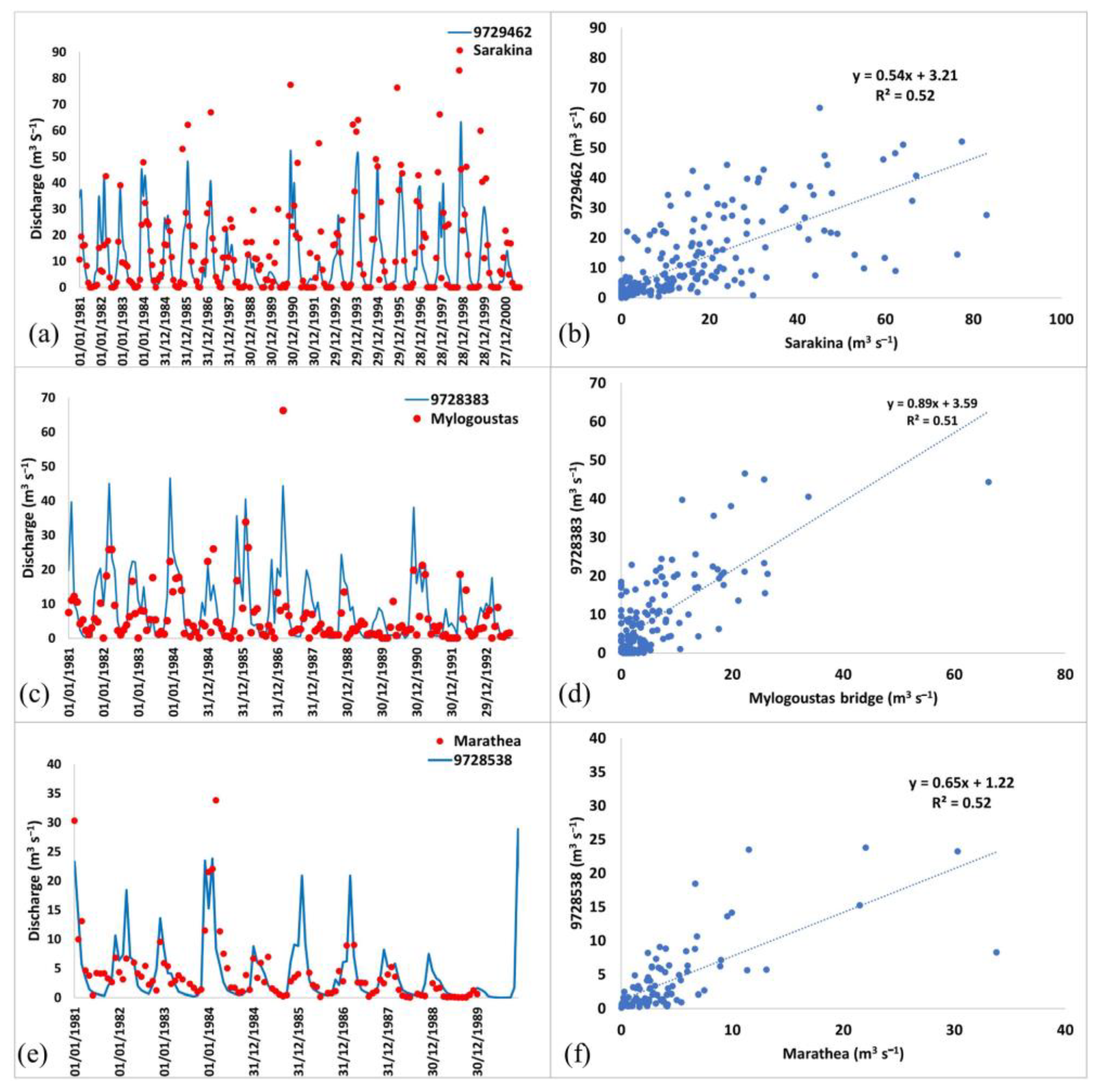
3.1. Evaluation of E-HYPE Data Using Measurements

Table 3 presents the statistical characteristics and the efficiency criteria considered for the evaluation of monthly discharges simulated by the hydrological model E-HYPE using measured discharges. Based on the results, in all cases, the correlation coefficient R can be characterized as high, based on previously proposed criteria for correlation interpretation [80], indicating sufficient performance for the model. The NSE was in all cases positive, and in sub-basins PINUP and MREMA, near 0.50, which is considered indicative of satisfactory model performance. Additionally, RSR was lower than 0.70 in all cases, and PBIAS was 22% in the case of the PINUP sub-basin. Overall, the model performance at PINUP and MREMA sub-basins can be considered satisfactory (Table 3, Figure A1). The performance in sub-basin TITAR is acceptable, although it is characterized by low NSE and quite a negative PBIAS that could be partially attributed to the increased altitude gradient of this sub-basin (Table 1).

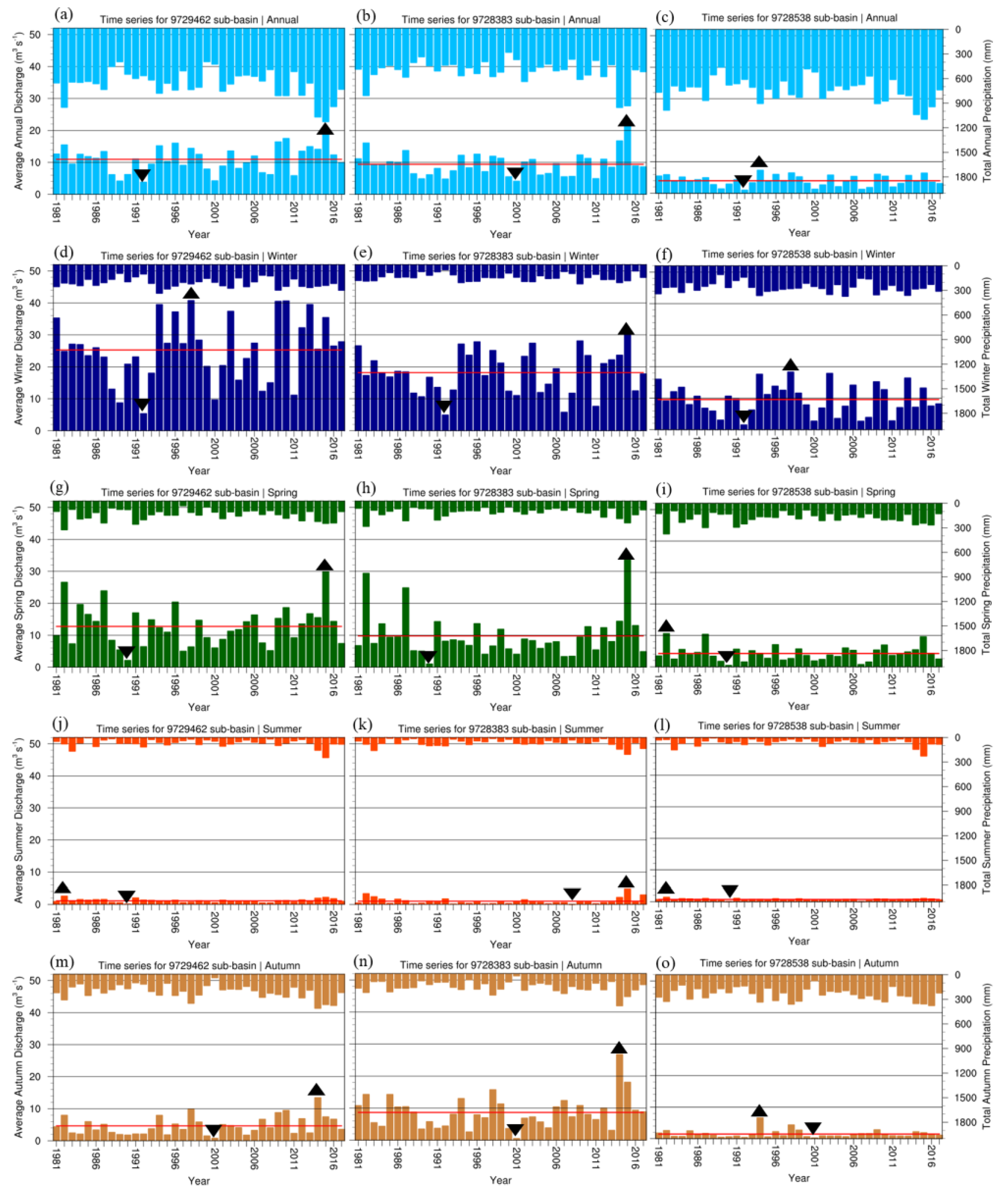
3.2. Interannual Distribution of Average Annual and Seasonal Discharge

After the statistical evaluation of the model data, we constructed time series of average annual and seasonal discharge from 1981 to 2017 for the three sub-basins (PINUP, TITAR, and MREMA) (Figure 2). Then, we estimated annual and seasonal maximum, minimum, and average discharge values in the three sub-basins for the 37-year period from 1981 to 2017 (Figure 2).
In more detail, Figure 2a–c presents time series of average annual discharge for the three sub-basins. To facilitate the interpretation of temporal variabilities of discharge, the respective time series of total annual precipitation is also illustrated. The results of this first analysis show that the average annual discharge in the three sub-basins is characterized by high temporal variabilities over the years. This indicates that the upstream Pinios river basin is strongly affected by large-scale temporal variabilities in precipitation that determine water runoff and discharge. Indeed, the Pinios basin is included in the wider region of Greece and the southern Balkans, which is characterized by large interannual and interdecadal variabilities in precipitation during the last decades, as noted by previous studies [4,19,22,81]. The interannual and interdecadal variabilities in precipitation are mostly determined by the large-scale variabilities of the atmospheric circulation bringing precipitation systems to the area and, thus, influencing the alteration between dry and wet periods [20,21,82,83,84].
The 37-year average discharges in the three sub-basins (PINUP, TITAR, and MREMA) are 11, 9.4, and 4 m3 s−1, respectively (Figure 2a–c). The discharge differences among the sub-basins are mostly attributed to the respective differences in their total area, altitude distribution, and location (Figure 1 and Table 1) that impact the precipitation amount received [4,26,44] and, thus, the discharge. The PINUP sub-basin has the largest average discharge because its western part is well located in the Pindus mountain range, which receives the most precipitation in Greece compared with other areas [85].
The average seasonal discharges in the three sub-basins (PINUP, TITAR, and MREMA) present high seasonality, as shown in Figure 2d–o. They are characterized by high variabilities between the seasons, presenting maxima in winter (December, January, and February—DJF), smaller values in spring (March, April, and May—MAM), even smaller values in autumn (September, October, and November—SON) and minima in summer (June, July, and August—JJA). For example, the maximum average discharge in the PINUP sub-basin for winter was estimated to be 40.7 m3 s−1 in 1998 (Figure 2d). However, the minimum one for summer reached about 0.1 m3 s−1 in 1990 (Figure 2j). Similar seasonal variabilities are demonstrated for all the sub-basins, mainly driven by the respective precipitation variabilities (Figure 2d–o). It is noteworthy that overall, 1990 and 1992 can be characterized as the driest years of the 37-year period studied (Figure 2). This is explained by the large-scale decrease in precipitation (depicted in Figure 2) and drought that influenced this period not only Pinios basin [23,24] but also in the eastern Mediterranean region [17,18,20].

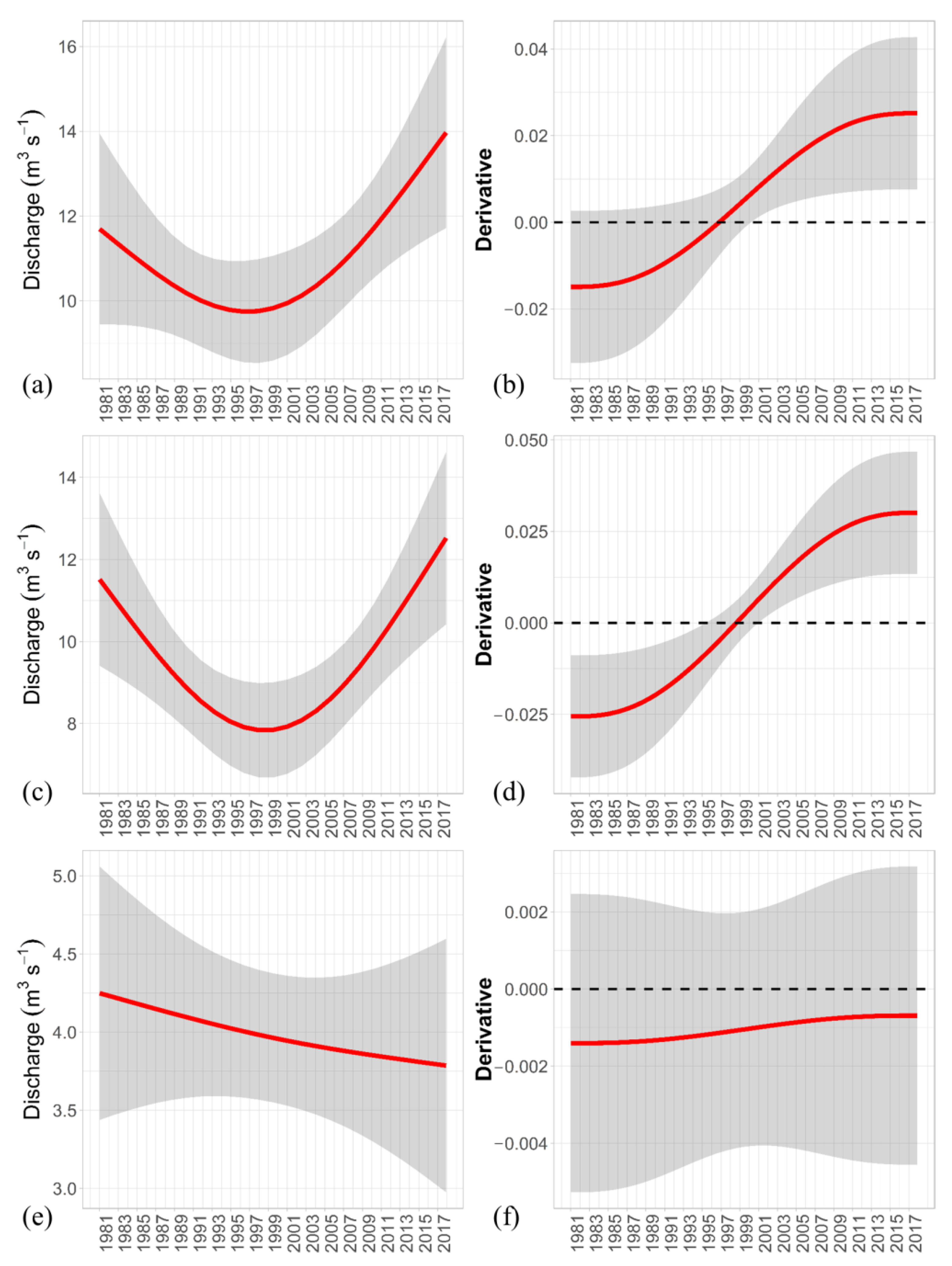
3.3. Generalized Additive Model Results

This sub-section presents a fit of the interannual trends of discharges of the three studied sub-basins using GAMs. Statistically significant non-linear trends of the monthly discharges were found for the sub-basins PINUP and TITAR (Table 4). In both sub-basins, discharge appears to decline from approximately 12 m3 s−1 in 1981 to below 10 and 8 m3 s−1, respectively, in 1997, and then it increases to 14 m3 s−1 and a little above 12 m3 s−1 in 2017 (Figure 3a,c). This pattern is also shown in Figure 3b,d, where the negative rates of change for sub-basins PINUP and TITAR decrease until 1997 and then rise until 2017. On the other hand, although there are no statistically significant trends in the MREMA sub-basin (Figure 3e,f), a declining linear trend is presented, probably due to its relatively increased agriculture (Table 1) that implies irrigation effects, thus complicating the investigation of pure climatic trends. When examining the trends separately for each month, significant interannual trends were noted only for September for sub-basins PINUP and TITAR, following the same pattern as described previously (Table 4, Figure 4), although it is obvious that the discharges were relatively low in 1981 (around 1 m3 s−1 for both sub-basins). It is noteworthy that sub-basin TITAR showed a sharp increase in the discharge, compared to the sub-basin PINUP, reaching 8 m3 s−1 in 2017 with a large rate of change. Therefore, September was wetter in the 2000s and 2010s compared to the 1980s and 1990s. This increasing interannual trend in the discharge of September is an interesting finding because the rivers in Greece are in their driest condition in September.

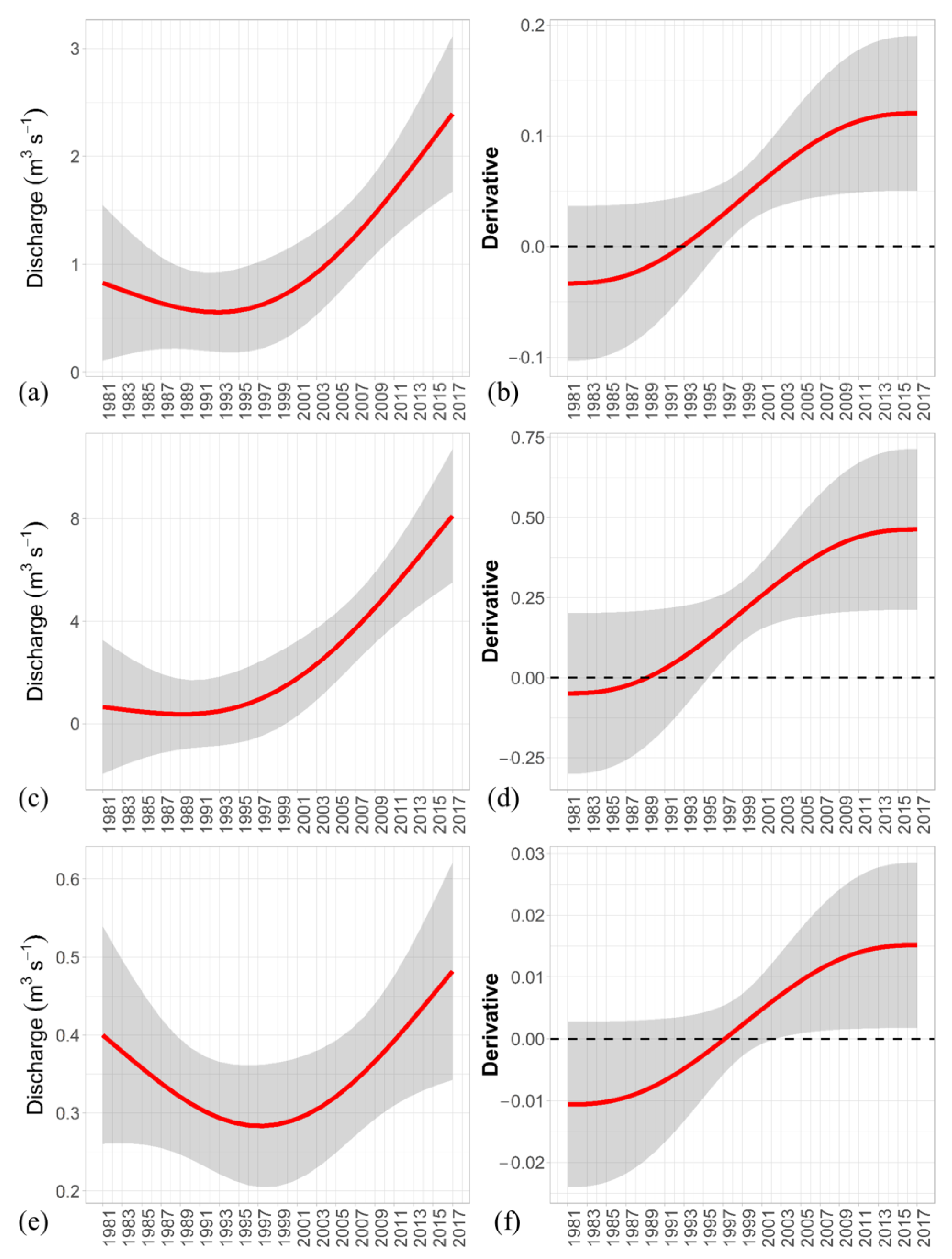
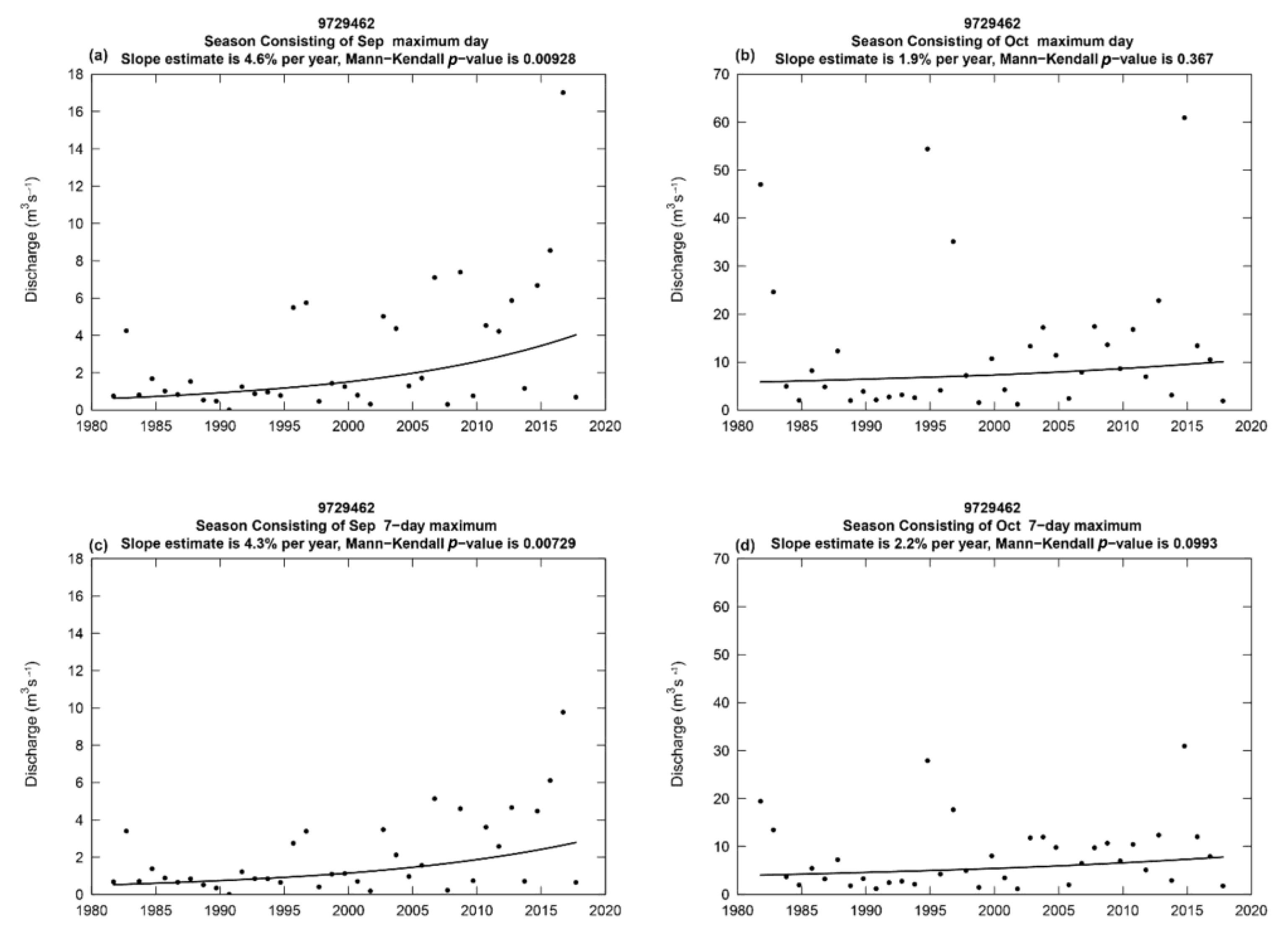
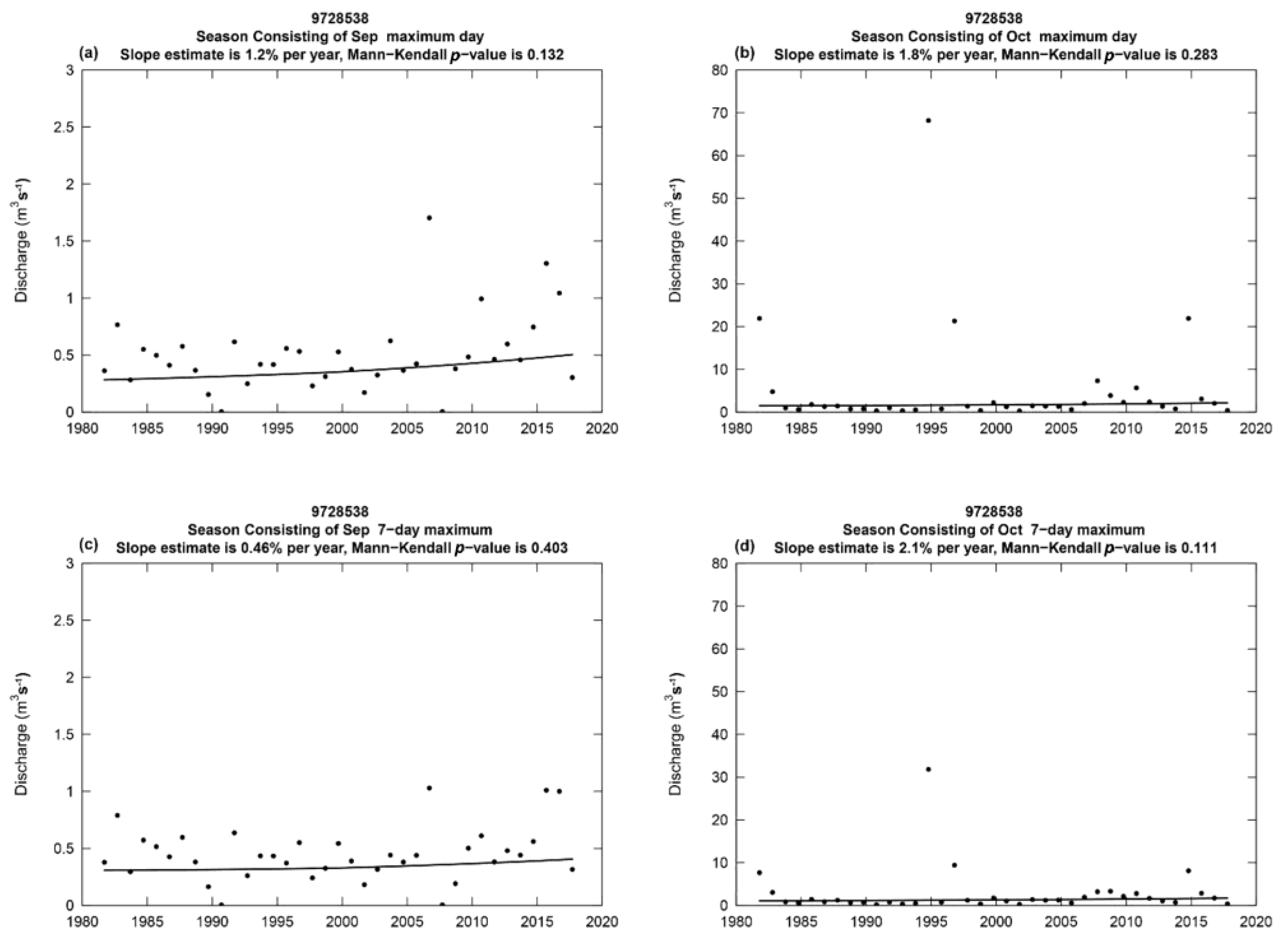
3.4. Interannual Increasing Trends of Discharge Maxima

Maximum analyses were conducted for every month of the year as well as for the selected period from July to October, aiming at untangling the interannual effects on discharge maxima. Only the statistically significant results with over 95% confidence level and some additional interesting results are presented here (Figure 5 and Figure 6). The graphical depiction of the history of high discharge statistics provided in Figure 5 and Figure 6 is an indication of the interannual changes in the magnitude of discharge events in the sub-basins PINUP, TITAR, and MREMA.
Results from the 4-month (July to October) analysis for the three sub-basins are presented side by side to facilitate the comparison (Figure 5). Increasing trends (represented by slopes) reaching 2.4% per year are apparent for the TITAR and PINUP sub-basins (Figure 5a–d). However, the trends are statistically significant in the 95% confidence level (p-value < 0.05) for both maximum 7-day and 30-day average discharges only for the TITAR sub-basin (Figure 5c,d). On the other hand, there is no significant trend (p-value > 0.1) at the sub-basin MREMA for both hydrological parameters (Figure 5e,f).
Based on the above results, further analysis was made to investigate changes in high flows employing a more detailed temporal resolution in the calculation of hydrological indices for each month. The analysis for maximum 1-day and 7-day average discharges resulted in statistically significant (p-value < 0.05) interannual trends only for September, while the results for October are interesting despite the fact that they are not statistically significant (Figure 6, Figure A2 and Figure A3). Therefore, the results only for these two months are presented in this sub-section. Figure 6, Figure A2 and Figure A3 consist of two hydrological variables (maximum 1-day and 7-day average discharges) describing discharge history relative to high flows that provide valuable information regarding long-term discharge modifications of the studied sub-basins throughout September and October.
One of the most substantial results of this study is that positive statistically significant trends of 10% per year in the slope of the maximum 1-day and 7-day average discharge were estimated for September in the TITAR sub-basin (Figure 6a,c). The PINUP sub-basin is characterized by smaller positive significant trends of 4.6% and 4.3% per year, respectively (Figure A2a,c). Given this information, it is reasonable to assume that the trend in discharge across September’s discharge distribution is positive and of substantial magnitude, particularly for the upper extremes of the discharge distribution. This result indicates that an interannual increasing trend in September’s precipitation maxima hides behind the corresponding increase of discharge maxima since the sub-basins were selected to be upstream and anthropogenically low affected. Positive trends in September are critical because this month is one of the driest months in Pinios river, and thus, the estimated interannual increase in discharge maxima has significant implications. Regarding October, increasing trends are shown, but they are not statistically significant (Figure 6b,d and Figure A2b,d). Nevertheless, it should be noted that the highest maximum discharge value (188 m3 s−1) among the three sub-basins occurred in TITAR sub-basin in October 2014 (Figure 6b).
As far as the sub-basin MREMA is concerned, there are no significant trends for the examined hydrological indices in both September and October (Figure A3a–d). This may be attributed to the fact that in contrast to the other two sub-basins, PINUP and TITAR, the MREMA sub-basin is not characterized by high altitudes (Table 1) that favor precipitation. In addition, MREMA also includes a considerable agricultural area that impacts the simulated discharges through the introduction of parameterized irrigation demands in the model. These two factors have direct and indirect effects on the discharge regime, and thus, they cause inhomogeneities in the prevailing climatic trends of discharge in the upstream region of the Pinios river basin.
The magnitude of the trends across the range from low to high flows is demonstrated in Quantile-Kendall plots for the three sub-basins for September and October (Figure 7). The overall variability of September’s discharge in all sub-basins has generally been increasing over time. Trends near the medians of the discharge distributions tend to be smaller positive values than the trends at the higher discharges for September, while the opposite occurs in October. For the highest flow days of September, across the probability distribution, the changes are statistically significant, especially for the sub-basins PINUP (Figure 7a,b) and TITAR (Figure 7c,d), whereas the upper quartile of the daily discharge distribution shows very likely to highly likely positive trends, typically above the range of 4% per year. Between the median and the 99th percentile of the distribution, discharges show a decline, least substantial (nevertheless, the trends are classified as likely downwards), for October. Trends in the range of low flows of the discharge distributions tend to be smaller positive values than the trends at the higher discharges with no significant increasing trends, except the PINUP sub-basin in October.

4. Discussion

4.1. Climate Change Effects on Discharge Maxima in Early Autumn

Climate change should be considered as a main driver of change in the temporal distribution of water availability, affecting the magnitude and frequency of both precipitation and discharge maxima. The results of the present study highlighted an important aspect of rapid climate change during the last four decades regarding water resources by reporting significantly increasing trends in early-autumn discharge maxima in the TITAR and PINUP sub-basins during the period 1981–2017. Our study agrees, especially regarding September, with a previous study [36] mentioning that the total annual number of flood occurrences in Pinios presented an increasing trend from 1990 to 2010. Our findings also corroborate the latest knowledge of the scientific community, such as that presented in the IPCC Sixth Assessment Report [7], showcasing the triggering role of climate change on extreme hydrometeorological events that are frequently associated with discharge extremes. The substantial increasing trends in discharge maxima presented here are strongly dependent on climate change effects on the water cycle that bridges rivers with climate-related increases in precipitation maxima [7]. Several studies have shown that heavy precipitation events are influenced by various climate change-induced atmospheric parameters such as temperature, due point temperature, moisture, and wind but also sea parameters such as sea surface temperature and sea surface roughness [38,86,87,88]. Albeit there are large uncertainties in climate change effects on precipitation, it is important to note that atmospheric moisture is considered the most significant factor for the increase in short-duration precipitation extreme events. This is attributed to the fact that climate change strongly affects atmospheric moisture content with an increase of 7% per 1 °C of air temperature increase [89].
Our findings indicate that modeled discharge data can facilitate the scope of this study, as they are generally in good agreement with measurements. More specifically, average seasonal discharges in the three sub-basins (PINUP, TITAR, and MREMA) present high seasonality, whereas statistically significant non-linear trends of the monthly discharges were found for the sub-basins PINUP and TITAR. Based on the above results, further analysis was made to investigate changes in high flows employing a more detailed temporal resolution. One of the most substantial results of this study is that in comparison with other months, September has positive statistically significant interannual trends for the TITAR and PINUP sub-basins. September’s increase in discharge maxima could imply a climate-induced increase in precipitation maxima in the Pinios river basin, as the two abovementioned sub-basins were selected to be upstream, partially mountainous, and anthropogenically low impacted. Moreover, given the fact that global warming enhances evapotranspiration, thus reducing water on the ground, the role of precipitation in increasing September’s discharge maxima is critical. It is well-known that heavy precipitation events are largely dependent on energy and moisture content in the atmosphere. For example, high moisture amounts favoring such precipitation events in the Pinios basin and generally in Greece, are usually originated from the Aegean and Ionian Seas [32,34,38]. A warmer Mediterranean Sea during the last decades could positively contribute to the formation of high-energy and high-moisture atmospheric systems such as “medicanes”. Ianos medicane, which occurred in September 2020, is a typical example of the abovementioned processes. Ianos formed in September when the Mediterranean Sea was still warm enough. However, the atmosphere began to cool down by southward movements of relatively colder air masses from northern-central Europe. This enhancement in the sea-air temperature contrast is a significant factor, and it hides behind the formation of Ianos. Thus, Ianos brought vast amounts of energy and moisture from the sea that triggered heavy rainfall that caused flash floods in southwestern parts of the Pinios river basin [35,90]. An interpretation of our findings reveals a connection between such phenomena, which could be more frequent in a warmer future climate, and, thus, more research in their hydrometeorological aspects and implications is needed, additionally considering potential climate change effects [91]. In this context, co-analyses between discharge, precipitation, and evapotranspiration during the last decades as well as in-depth analyses of extreme precipitation events in the Pinios basin driving to flash floods (e.g., that caused by the Ianos medicane in 2020), are interesting proposals for future research.

4.2. Necessity for Untangling Climate Effects and Direct Anthropogenic Pressures

This study focused on the unraveling of interannual variabilities and trends of annual average discharge and discharge maxima during the period from 1981 to 2017, avoiding parts of the Pinios river basin that are characterized by increased agricultural activity. However, the Pinios river basin is one of the most productive areas of the country regarding the agricultural sector, also including multiple anthropogenic pressures [45] such as big cities (e.g., Larissa city with more than 140,000 residents), irrigation processes, bridges, technical works, industries, buildings, pollution, etc. Thus, the results of the present study regarding the upstream of the river may deviate from low-lying areas. For example, the analyses showed an increase in an annual average discharge after the middle 1990s in the upstream sub-basins. However, this increase could be eliminated in lowlands if considering a probable increase in irrigation, removing water from the river and transferring it to the fields, or changes in land use. These factors are significant because agriculture had an increasing trend, especially in the 1990s in the Pinios basin, also presenting land use changes.
Additionally, the increase in temperature since the 1990s, especially during summer, could have impacts on the increasing irrigation demands [25]. Ε-HYPE has sufficiently considered irrigation [55,56] and crop water demand [57]. Nevertheless, the combination of the abovementioned factors poses the necessity to dynamically consider the changes in irrigation and land use in low-lying sub-basins as well as the installation of small dams if the aim is to investigate the effects of both climate change and direct anthropogenic pressures on discharge. Such an effort presupposes a lot of detailed spatiotemporally distributed information about factors such as irrigation, land use, and dams, which is very difficult to find and introduce every year in the estimation of the hydrological cycle by the hydrological model. It is nevertheless a suggestion for future work in the Pinios river basin aiming for a more holistic approach to the issue of simulated long-term discharge trends in the whole river.

5. Conclusions

The scope of the present study was to investigate variabilities and significant interannual trends in the annual average discharge of three upstream sub-basins of the Pinios river while also unraveling significant trends in discharge maxima by examining each month. To this aim, daily discharges from the E-HYPE model from 1981 to 2017 were used. The most critical conclusions of this study are summarized below:
  • The analysis of data revealed noteworthy findings for the upstream Pinios river. The average annual discharge in the three sub-basins decreased in the 1980s, reaching a minimum in the early 1990s when extensive droughts influenced not only Pinios river but also several areas of the Mediterranean region. Afterward, the average annual discharge gradually increased from the middle 1990s to 2017, reaching approximately the discharge levels of the early 1980s.
  • The interannual and interdecadal discharge variabilities presented in this study were characterized by high amplitudes. These variabilities were induced by large-scale climatic forcings that largely determined the water resources of the Pinios river basin.
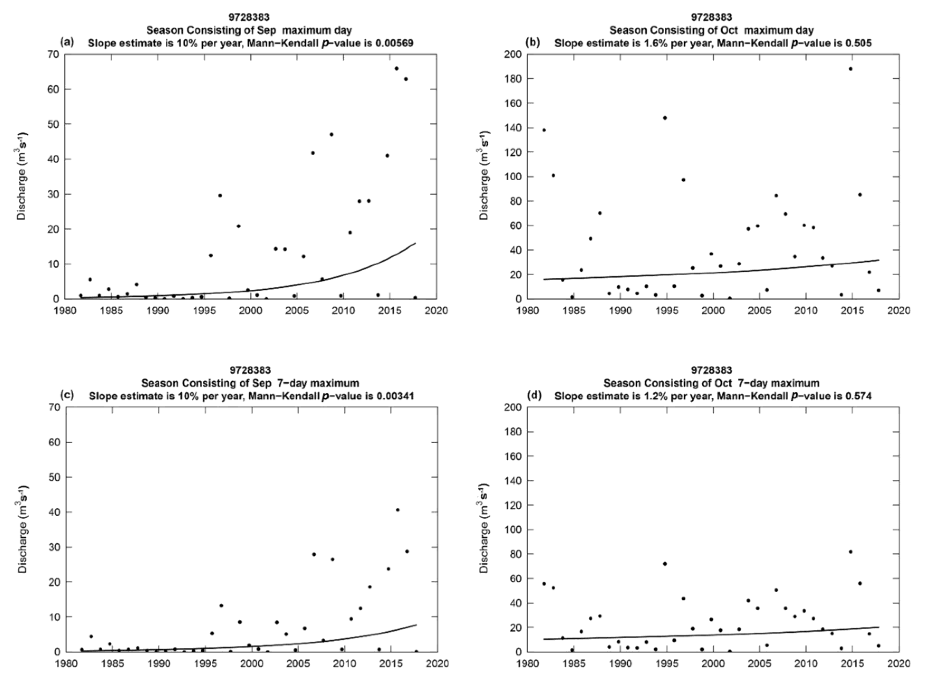
  • The most striking finding of this study is that significantly increasing interannual trends in discharge maxima were identified for September, which is one of the driest months in the Pinios river basin. The performed discharge history analyses indicated the presence of large positive (10% and approximately 4.5% per year for TITAR and PINUP sub-basins, respectively) statistically significant (p-value < 0.05) interannual trends in maximum 1-day and 7-day average discharges for September.
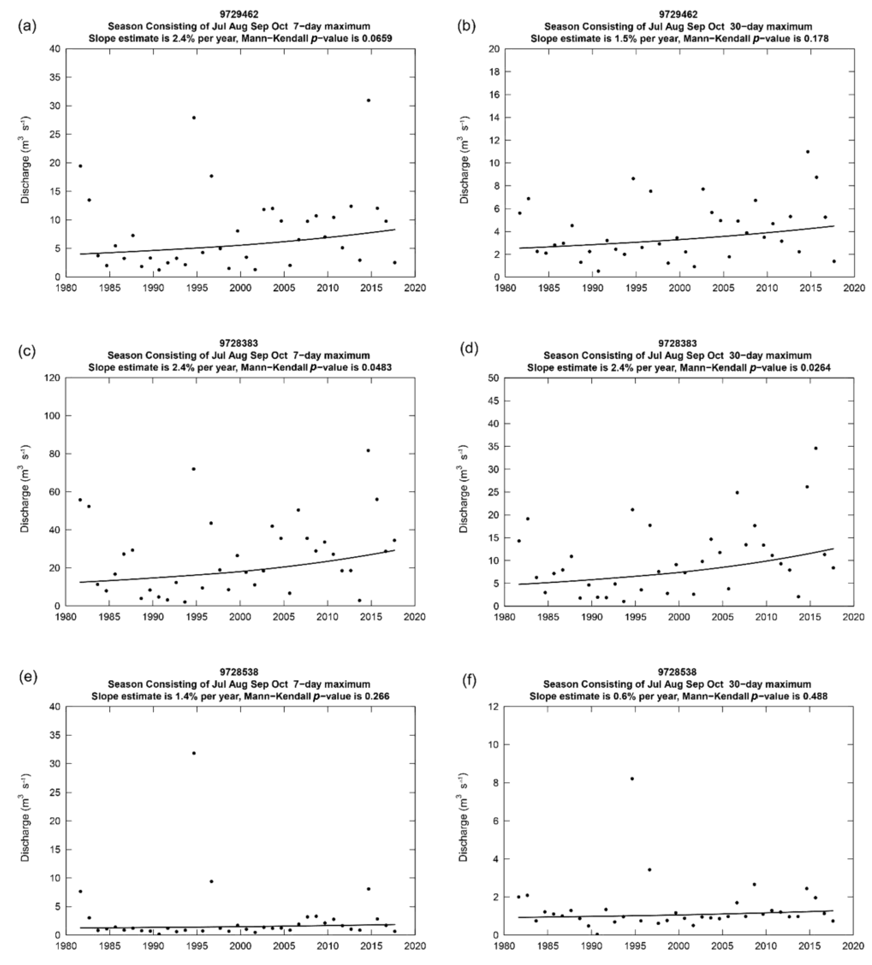
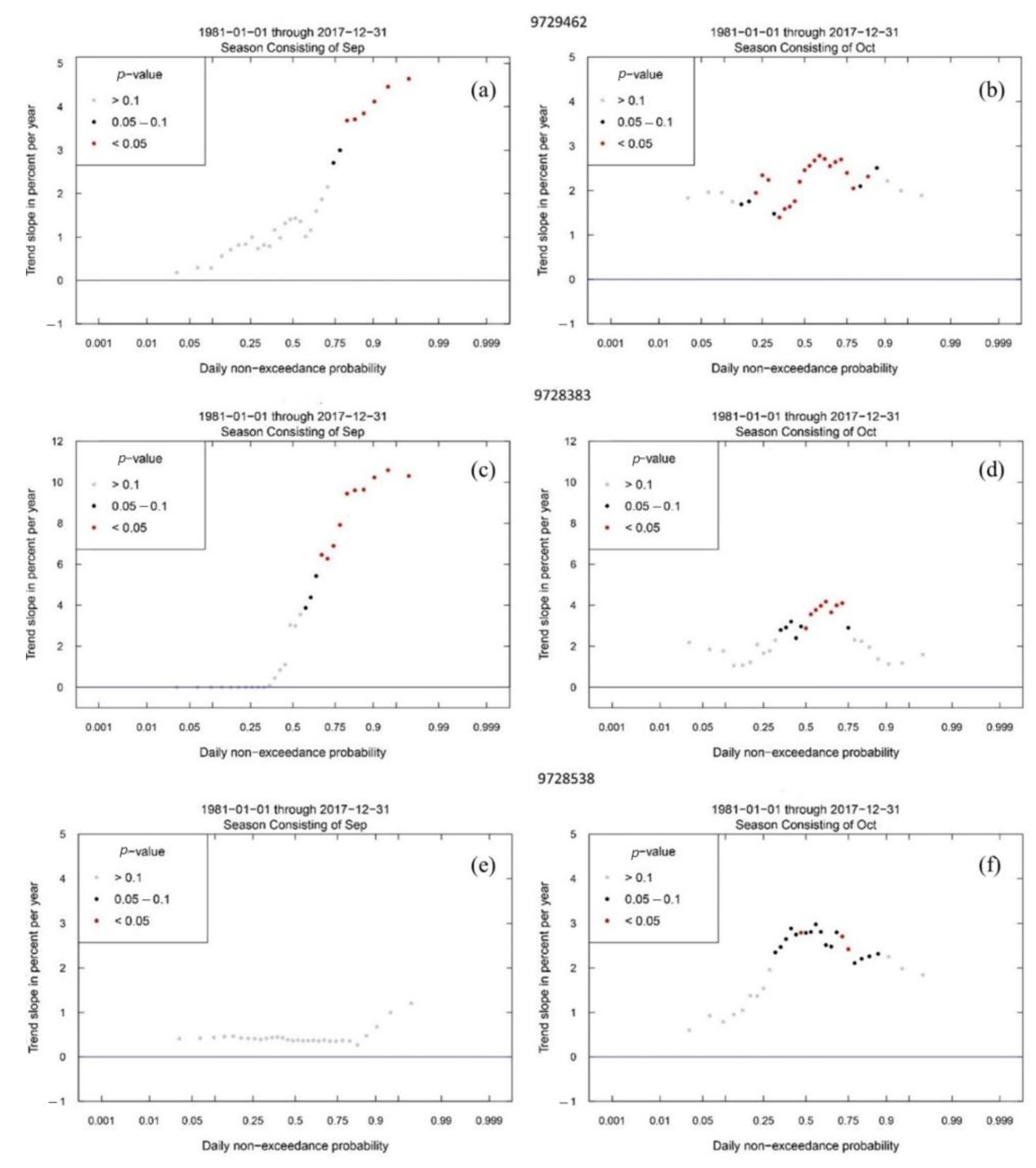
  • The increases in high flows were also much more substantial than those near the median flows for September, as evidenced by Quantile-Kendall plots. Significant increasing trends up to 2.4 per year for the TITAR sub-basin were also resulted by analyzing maximum 7-day and 30-day average discharges considering the period from July to October.
The findings of this study regarding the interannual trends of both the annual average discharge and discharge maxima can be exploited by the scientific community to conduct climate studies as well as interdisciplinary projects. The implications of large variabilities in discharge over the years are related to multi-year wet and dry periods that influence the society, economy, and ecosystems of the Pinios basin. The increase of discharge maxima in early autumn, when the rivers in Greece are in their driest condition, is a clear signal of climate change that must be seriously considered in the future. The increase in maxima may potentially determine suitable hydrological conditions for the increased probability of floods during late summer and especially early autumn periods. This study presents a paradigm for probable discharge variabilities in the future, and thus, decision-makers and civil protection may consider the results when they make basin management strategies as well as climate change adaptation and mitigation plans.

Author Contributions

Conceptualization, G.V., C.P., K.S. and A.M.; methodology, G.V., C.P., K.S. and A.M.; software, G.V., C.P., K.S. and A.M.; validation, G.V. and A.M.; formal analysis, G.V., C.P., K.S., A.M., I.P., A.P. and E.D.; investigation, G.V., C.P., K.S., A.M., I.P., A.P. and E.D.; resources, I.P., A.P. and E.D.; data curation, G.V., C.P., K.S., A.M. and I.P.; writing—original draft preparation, G.V., C.P., K.S., A.M. and I.P.; writing—review and editing, G.V., C.P., K.S., A.M., I.P., A.P. and E.D.; visualization, G.V., C.P., K.S. and A.M.; supervision, A.P. and E.D.; project administration, G.V. All authors have read and agreed to the published version of the manuscript.

Funding

This research received no external funding.

Institutional Review Board Statement

Not applicable.

Informed Consent Statement

Not applicable.

Data Availability Statement

The data presented in this study are available on request from the corresponding author.

Acknowledgments

The European Hydrological Predictions for the Environment (E-HYPE) model climate dataset, including average daily discharge values from 1 January 1981 to 31 December 2017, was kindly provided by the Hydrological Research Unit at the Swedish Meteorological and Hydrological Institute (SMHI). Time series and maps from the E-HYPE model are available for inspection at http://hypeweb.smhi.se, accessed on 5 March 2023.

Conflicts of Interest

The authors declare no conflict of interest.

Appendix A

Statistical criteria of the E-HYPE model performance by comparing observed (o) and modeled (m) data of a sample size (n):
Pearson’s correlation coefficient ( R ).
R = i = 1 n ( m i m ¯ ) ( o i o ¯ ) i = 1 n ( m i m ¯ ) 2 i = 1 n ( o i o ¯ ) 2
Percent bias ( P B I A S ).
P B I A S = 100 × i = 1 n ( o i m i ) i = 1 n o i
Root mean square error ( R M S E ).
R M S E = i = 1 n ( o i m i ) 2 n
Ratio of the RMSE to the Standard Deviation of observations ( R S R ).
R S R = i = 1 n ( o i m i ) 2 i = 1 n ( o i o ¯ ) 2
Nash-Sutcliffe efficiency ( N S E ).
N S E = 1 i = 1 n ( o i m i ) 2 i = 1 n ( o i o ¯ ) 2
Figure A1. Simulated and measured discharge (m3 s−1) values and correlations of (a,b) PINUP—Sarakinas bridge, (c,d) TITAR—Mylogoustas bridge, and (e,f) MREMA—Marathea station.
Water 15 01022 g0a1
Figure A2. Trends of maximum 1-day and 7-day average discharges in the PINUP sub-basin during the period 1981–2017 for September (a,c) and October (b,d), respectively. A Thiel-Sen slope and a two-sided p-value for the Mann-Kendall trend test are also presented in the graphs.
Water 15 01022 g0a2
Figure A3. Trends of maximum 1-day and 7-day average discharges in the MREMA sub-basin during the period 1981–2017 for September (a,c) and October (b,d), respectively. A Thiel-Sen slope and a two-sided p-value for the Mann-Kendall trend test are also presented in the graphs.
Water 15 01022 g0a3

References

  1. Gudmundsson, L.; Boulange, J.; Do, H.X.; Gosling, S.N.; Grillakis, M.G.; Koutroulis, A.G.; Leonard, M.; Liu, J.; Schmied, H.M.; Papadimitriou, L.; et al. Globally Observed Trends in Mean and Extreme River Flow Attributed to Climate Change. Science 2021, 371, 1159–1162. [Google Scholar] [CrossRef]
  2. Arnell, N.W.; Gosling, S.N. The Impacts of Climate Change on River Flood Risk at the Global Scale. Clim. Chang. 2016, 134, 387–401. [Google Scholar] [CrossRef] [Green Version]
  3. Giorgi, F. Climate Change Hot-Spots. Geophys. Res. Lett. 2006, 33, 8707. [Google Scholar] [CrossRef]
  4. Varlas, G.; Stefanidis, K.; Papaioannou, G.; Panagopoulos, Y.; Pytharoulis, I.; Katsafados, P.; Papadopoulos, A.; Dimitriou, E. Unravelling Precipitation Trends in Greece since 1950s Using ERA5 Climate Reanalysis Data. Climate 2022, 10, 12. [Google Scholar] [CrossRef]
  5. Mentzafou, A.; Varlas, G.; Dimitriou, E.; Papadopoulos, A.; Pytharoulis, I.; Katsafados, P. Modeling the Effects of Anthropogenic Land Cover Changes to the Main Hydrometeorological Factors in a Regional Watershed, Central Greece. Climate 2019, 7, 129. [Google Scholar] [CrossRef] [Green Version]
  6. Mentzafou, A.; Vamvakaki, C.; Zacharias, I.; Gianni, A.; Dimitriou, E. Climate Change Impacts on a Mediterranean River and the Associated Interactions with the Adjacent Coastal Area. Environ. Earth Sci. 2017, 76, 259. [Google Scholar] [CrossRef]
  7. Masson-Delmotte, V.; Zhai, P.; Chen, Y.; Goldfarb, L.; Gomis, M.I.; Matthews, J.B.R.; Berger, S.; Huang, M.; Yelekçi, O.; Yu, R.; et al. Contribution to the Sixth Assessment Report of the Intergovernmental Panel on Climate Change; Cambridge University Press: Cambridge, UK; New York, NY, USA, 2021. [Google Scholar]
  8. Masseroni, D.; Camici, S.; Cislaghi, A.; Vacchiano, G.; Massari, C.; Brocca, L. The 63-Year Changes in Annual Streamflow Volumes across Europe with a Focus on the Mediterranean Basin. Hydrol. Earth Syst. Sci. 2021, 25, 5589–5601. [Google Scholar] [CrossRef]
  9. Blöschl, G.; Hall, J.; Viglione, A.; Perdigão, R.A.P.; Parajka, J.; Merz, B.; Lun, D.; Arheimer, B.; Aronica, G.T.; Bilibashi, A.; et al. Changing Climate Both Increases and Decreases European River Floods. Nature 2019, 573, 108–111. [Google Scholar] [CrossRef]
  10. Montaldo, N.; Oren, R. Changing Seasonal Rainfall Distribution With Climate Directs Contrasting Impacts at Evapotranspiration and Water Yield in the Western Mediterranean Region. Earth’s Future 2018, 6, 841–856. [Google Scholar] [CrossRef]
  11. Brogli, R.; Sørland, S.L.; Kröner, N.; Schär, C. Causes of Future Mediterranean Precipitation Decline Depend on the Season. Environ. Res. Lett. 2019, 14, 114017. [Google Scholar] [CrossRef]
  12. Giannakopoulos, C.; Kostopoulou, E.; Varotsos, K.V.; Tziotziou, K.; Plitharas, A. An Integrated Assessment of Climate Change Impacts for Greece in the near Future. Reg. Environ. Chang. 2011, 11, 829–843. [Google Scholar] [CrossRef] [Green Version]
  13. Sellami, H.; Benabdallah, S.; La Jeunesse, I.; Vanclooster, M. Quantifying Hydrological Responses of Small Mediterranean Catchments under Climate Change Projections. Sci. Total Environ. 2016, 543, 924–936. [Google Scholar] [CrossRef] [PubMed]
  14. Stefanidis, K.; Panagopoulos, Y.; Mimikou, M. Response of a Multi-Stressed Mediterranean River to Future Climate and Socio-Economic Scenarios. Sci. Total Environ. 2018, 627, 756–769. [Google Scholar] [CrossRef]
  15. Papadaki, C.; Soulis, K.; Muñoz-Mas, R.; Martinez-Capel, F.; Zogaris, S.; Ntoanidis, L.; Dimitriou, E. Potential Impacts of Climate Change on Flow Regime and Fish Habitat in Mountain Rivers of the South-Western Balkans. Sci. Total Environ. 2016, 540, 418–428. [Google Scholar] [CrossRef] [Green Version]
  16. Panagopoulos, A.; Arampatzis, G.; Tziritis, E.; Pisinaras, V.; Herrmann, F.; Kunkel, R.; Wendland, F. Assessment of Climate Change Impact in the Hydrological Regime of River Pinios Basin, Central Greece. Desalination Water Treat. 2016, 57, 2256–2267. [Google Scholar] [CrossRef]
  17. Feidas, H.; Noulopoulou, C.; Makrogiannis, T.; Bora-Senta, E. Trend Analysis of Precipitation Time Series in Greece and Their Relationship with Circulation Using Surface and Satellite Data: 1955–2001. Theor. Appl. Climatol. 2007, 87, 155–177. [Google Scholar] [CrossRef]
  18. Hatzianastassiou, N.; Katsoulis, B.; Pnevmatikos, J.; Antakis, V. Spatial and Temporal Variation of Precipitation in Greece and Surrounding Regions Based on Global Precipitation Climatology Project Data. J. Clim. 2008, 21, 1349–1370. [Google Scholar] [CrossRef]
  19. Nastos, P.T.; Zerefos, C.S. Spatial and Temporal Variability of Consecutive Dry and Wet Days in Greece. Atmos. Res. 2009, 94, 616–628. [Google Scholar] [CrossRef]
  20. Hurrell, J.W. Decadal Trends in the North Atlantic Oscillation: Regional Temperatures and Precipitation. Science 1995, 269, 676–679. [Google Scholar] [CrossRef] [Green Version]
  21. Xoplaki, E.; González-Rouco, J.F.; Luterbacher, J.; Wanner, H. Wet Season Mediterranean Precipitation Variability: Influence of Large-Scale Dynamics and Trends. Clim. Dyn. 2004, 23, 63–78. [Google Scholar] [CrossRef] [Green Version]
  22. Philandras, C.M.; Nastos, P.T.; Kapsomenakis, J.; Douvis, K.C.; Tselioudis, G.; Zerefos, C.S. Long Term Precipitation Trends and Variability within the Mediterranean Region. Nat. Hazards Earth Syst. Sci. 2011, 11, 3235–3250. [Google Scholar] [CrossRef] [Green Version]
  23. Vasiliades, L.; Loukas, A. Hydrological Response to Meteorological Drought Using the Palmer Drought Indices in Thessaly, Greece. Desalination 2009, 237, 3–21. [Google Scholar] [CrossRef]
  24. Loukas, A.; Vasiliades, L. Probabilistic Analysis of Drought Spatiotemporal Characteristics InThessaly Region, Greece. Nat. Hazards Earth Syst. Sci. 2004, 4, 719–731. [Google Scholar] [CrossRef]
  25. Mentzafou, A.; Dimitriou, E.; Papadopoulos, A. Long-Term Hydrologic Trends in the Main Greek Rivers: A Statistical Approach. In Handbook of Environmental Chemistry; Springer: Berlin, Heidelberg, 2015; Volume 59, pp. 129–165. [Google Scholar]
  26. Loukas, A. Surface Water Quantity and Quality Assessment in Pinios River, Thessaly, Greece. Desalination 2010, 250, 266–273. [Google Scholar] [CrossRef]
  27. Zittis, G.; Bruggeman, A.; Lelieveld, J. Revisiting Future Extreme Precipitation Trends in the Mediterranean. Weather Clim. Extrem. 2021, 34, 100380. [Google Scholar] [CrossRef] [PubMed]
  28. Camera, C.; Bruggeman, A.; Zittis, G.; Sofokleous, I.; Arnault, J. Simulation of Extreme Rainfall and Streamflow Events in Small Mediterranean Watersheds with a One-Way-Coupled Atmospheric-Hydrologic Modelling System. Nat. Hazards Earth Syst. Sci. 2020, 20, 2791–2810. [Google Scholar] [CrossRef]
  29. Spyrou, C.; Varlas, G.; Pappa, A.; Mentzafou, A.; Katsafados, P.; Papadopoulos, A.; Anagnostou, M.N.; Kalogiros, J. Implementation of a Nowcasting Hydrometeorological System for Studying Flash Flood Events: The Case of Mandra, Greece. Remote Sens. 2020, 12, 2784. [Google Scholar] [CrossRef]
  30. Varlas, G.; Anagnostou, M.N.; Spyrou, C.; Papadopoulos, A.; Kalogiros, J.; Mentzafou, A.; Michaelides, S.; Baltas, E.; Karymbalis, E.; Katsafados, P. A Multi-Platform Hydrometeorological Analysis of the Flash Flood Event of 15 November 2017 in Attica, Greece. Remote Sens. 2019, 11, 45. [Google Scholar] [CrossRef] [Green Version]
  31. Giannaros, C.; Dafis, S.; Stefanidis, S.; Giannaros, T.M.; Koletsis, I.; Oikonomou, C. Hydrometeorological Analysis of a Flash Flood Event in an Ungauged Mediterranean Watershed under an Operational Forecasting and Monitoring Context. Meteorol. Appl. 2022, 29, e2079. [Google Scholar] [CrossRef]
  32. Papaioannou, G.; Varlas, G.; Papadopoulos, A.; Loukas, A.; Katsafados, P.; Dimitriou, E. Investigating Sea-state Effects on Flash Flood Hydrograph and Inundation Forecasting. Hydrol. Process. 2021, 35, e14151. [Google Scholar] [CrossRef]
  33. Fowler, H.J.; Lenderink, G.; Prein, A.F.; Westra, S.; Allan, R.P.; Ban, N.; Barbero, R.; Berg, P.; Blenkinsop, S.; Do, H.X.; et al. Anthropogenic Intensification of Short-Duration Rainfall Extremes. Nat. Rev. Earth Environ. 2021, 2, 107–122. [Google Scholar] [CrossRef]
  34. Papaioannou, G.; Varlas, G.; Terti, G.; Papadopoulos, A.; Loukas, A.; Panagopoulos, Y.; Dimitriou, E. Flood Inundation Mapping at Ungauged Basins Using Coupled Hydrometeorological-Hydraulic Modelling: The Catastrophic Case of the 2006 Flash Flood in Volos City, Greece. Water 2019, 11, 2328. [Google Scholar] [CrossRef] [Green Version]
  35. Lagouvardos, K.; Karagiannidis, A.; Dafis, S.; Kalimeris, A.; Kotroni, V. Ianos—A Hurricane in the Mediterranean. Bull. Am. Meteorol. Soc. 2022, 103, E1621–E1636. [Google Scholar] [CrossRef]
  36. Bathrellos, G.D.; Skilodimou, H.D.; Soukis, K.; Koskeridou, E. Temporal and Spatial Analysis of Flood Occurrences in the Drainage Basin of Pinios River (Thessaly, Central Greece). Land 2018, 7, 106. [Google Scholar] [CrossRef] [Green Version]
  37. Romero, R.; Emanuel, K. Medicane Risk in a Changing Climate. J. Geophys. Res. Atmos. 2013, 118, 5992–6001. [Google Scholar] [CrossRef]
  38. Varlas, G.; Vervatis, V.; Spyrou, C.; Papadopoulou, E.; Papadopoulos, A.; Katsafados, P. Investigating the Impact of Atmosphere–Wave–Ocean Interactions on a Mediterranean Tropical-like Cyclone. Ocean Model. 2020, 153, 101675. [Google Scholar] [CrossRef]
  39. European Environment Agency Copernicus Land Monitoring Service 2018. CORINE Land Cover CLC2018 Version 2020_20u1. Available online: https://land.copernicus.eu/pan-european/corine-land-cover/clc2018 (accessed on 5 March 2023).
  40. Hellenic Statistical Authority of Greece Statistics-Gross Value Added by Industry. Available online: https://www.statistics.gr/en/statistics/-/publication/SEL45/2019 (accessed on 10 October 2022).
  41. Migiros, G.; Bathrellos, G.D.; Skilodimou, H.D.; Karamousalis, T. Pinios (Peneus) River (Central Greece): Hydrological—Geomorphological Elements and Changes during the Quaternary. Cent. Eur. J. Geosci. 2011, 3, 215–228. [Google Scholar] [CrossRef]
  42. Caputo, R.; Helly, B.; Rapti, D.; Valkaniotis, S. Late Quaternary Hydrographic Evolution in Thessaly (Central Greece): The Crucial Role of the Piniada Valley. Quat. Int. 2022, 635, 3–19. [Google Scholar] [CrossRef]
  43. Kottek, M.; Grieser, J.; Beck, C.; Rudolf, B.; Rubel, F. World Map of the Köppen-Geiger Climate Classification Updated. Meteorol. Z. 2006, 15, 259–263. [Google Scholar] [CrossRef]
  44. Mylopoulos, N.; Kolokytha, E.; Loukas, A.; Mylopoulos, Y. Agricultural and Water Resources Development in Thessaly, Greece in the Framework of New European Union Policies. Int. J. River Basin Manag. 2009, 7, 73–89. [Google Scholar] [CrossRef]
  45. Mentzafou, A.; Varlas, G.; Papadopoulos, A.; Poulis, G.; Dimitriou, E. Assessment of Automatically Monitored Water Levels and Water Quality Indicators in Rivers with Different Hydromorphological Conditions and Pollution Levels in Greece. Hydrology 2021, 8, 86. [Google Scholar] [CrossRef]
  46. U.S. Geological Survey. Shuttle Radar Topography Mission 1 Arc-Second Global; U.S. Geological Survey: Reston, VA, USA, 2017.
  47. Lindström, G.; Pers, C.; Rosberg, J.; Strömqvist, J.; Arheimer, B. Development and Testing of the HYPE (Hydrological Predictions for the Environment) Water Quality Model for Different Spatial Scales. Hydrol. Res. 2010, 41, 295–319. [Google Scholar] [CrossRef]
  48. Hundecha, Y.; Arheimer, B.; Donnelly, C.; Pechlivanidis, I. A Regional Parameter Estimation Scheme for a Pan-European Multi-Basin Model. J. Hydrol. Reg. Stud. 2016, 6, 90–111. [Google Scholar] [CrossRef] [Green Version]
  49. Donnelly, C.; Andersson, J.C.M.; Arheimer, B. Using Flow Signatures and Catchment Similarities to Evaluate the E-HYPE Multi-Basin Model across Europe. Hydrol. Sci. J. 2016, 61, 255–273. [Google Scholar] [CrossRef] [Green Version]
  50. Krysanova, V.; Vetter, T.; Eisner, S.; Huang, S.; Pechlivanidis, I.; Strauch, M.; Gelfan, A.; Kumar, R.; Aich, V.; Arheimer, B.; et al. Intercomparison of Regional-Scale Hydrological Models and Climate Change Impacts Projected for 12 Large River Basins Worldwide—A Synthesis. Environ. Res. Lett. 2017, 12, 105002. [Google Scholar] [CrossRef]
  51. Vetter, T.; Reinhardt, J.; Flörke, M.; van Griensven, A.; Hattermann, F.; Huang, S.; Koch, H.; Pechlivanidis, I.G.; Plötner, S.; Seidou, O.; et al. Evaluation of Sources of Uncertainty in Projected Hydrological Changes under Climate Change in 12 Large-Scale River Basins. Clim. Chang. 2017, 141, 419–433. [Google Scholar] [CrossRef]
  52. Pechlivanidis, I.G.; Arheimer, B.; Donnelly, C.; Hundecha, Y.; Huang, S.; Aich, V.; Samaniego, L.; Eisner, S.; Shi, P. Analysis of Hydrological Extremes at Different Hydro-Climatic Regimes under Present and Future Conditions. Clim. Chang. 2017, 141, 467–481. [Google Scholar] [CrossRef] [Green Version]
  53. Samaniego, L.; Kumar, R.; Breuer, L.; Chamorro, A.; Flörke, M.; Pechlivanidis, I.G.; Schäfer, D.; Shah, H.; Vetter, T.; Wortmann, M.; et al. Propagation of Forcing and Model Uncertainties on to Hydrological Drought Characteristics in a Multi-Model Century-Long Experiment in Large River Basins. Clim. Chang. 2017, 141, 435–449. [Google Scholar] [CrossRef]
  54. Berg, P.; Donnelly, C.; Gustafsson, D. Near-Real-Time Adjusted Reanalysis Forcing Data for Hydrology. Hydrol. Earth Syst. Sci. 2018, 22, 989–1000. [Google Scholar] [CrossRef] [Green Version]
  55. Wriedt, G.; van der Velde, M.; Aloe, A.; Bouraoui, F. A European Irrigation Map for Spatially Distributed Agricultural Modelling. Agric. Water Manag. 2009, 96, 771–789. [Google Scholar] [CrossRef]
  56. Siebert, S.; Döll, P.; Hoogeveen, J.; Faures, J.M.; Frenken, K.; Feick, S. Development and Validation of the Global Map of Irrigation Areas. Hydrol. Earth Syst. Sci. 2005, 9, 535–547. [Google Scholar] [CrossRef]
  57. Portmann, F.T.; Siebert, S.; Döll, P. MIRCA2000-Global Monthly Irrigated and Rainfed Crop Areas around the Year 2000: A New High-Resolution Data Set for Agricultural and Hydrological Modeling. Glob. Biogeochem. Cycles 2010, 24, 1–24. [Google Scholar] [CrossRef]
  58. European Environment Agency Corine Land Cover 2000 Coastline. Available online: http://www.eea.europa.eu/data-and-maps/data/corine-land-cover-2000-coastline/#tab-gis-data (accessed on 5 March 2023).
  59. Hundecha, Y.; Arheimer, B.; Berg, P.; Capell, R.; Musuuza, J.; Pechlivanidis, I.; Photiadou, C. Effect of Model Calibration Strategy on Climate Projections of Hydrological Indicators at a Continental Scale. Clim. Chang. 2020, 163, 1287–1306. [Google Scholar] [CrossRef]
  60. Kumar, R.; Livneh, B.; Samaniego, L. Toward Computationally Efficient Large-Scale Hydrologic Predictions with a Multiscale Regionalization Scheme. Water Resour. Res. 2013, 49, 5700–5714. [Google Scholar] [CrossRef]
  61. Pechlivanidis, I.G.; Arheimer, B. Large-Scale Hydrological Modelling by Using Modified PUB Recommendations: The India-HYPE Case. Hydrol. Earth Syst. Sci. 2015, 19, 4559–4579. [Google Scholar] [CrossRef] [Green Version]
  62. Samaniego, L.; Kumar, R.; Jackisch, C. Predictions in a Data-Sparse Region Using a Regionalized Grid-Based Hydrologic Model Driven by Remotely Sensed Data. Hydrol. Res. 2011, 42, 338–355. [Google Scholar] [CrossRef]
  63. Beven, K. Rainfall-Runoff Modelling: The Primer, 2nd ed.; John Wiley & Sons, Ltd.: Chichester, UK, 2012; ISBN 9780470714591. [Google Scholar]
  64. Pechlivanidis, I.G.; Jackson, B.M.; Mcintyre, N.R.; Wheater, H.S. Catchment Scale Hydrological Modelling: A Review of Model Types, Calibration Approaches and Uncertainty Analysis Methods in the Context of Recent Developments in Technology and Applications. Glob. NEST J. 2011, 13, 193–214. [Google Scholar]
  65. Moriasi, D.; Arnold, J.; van Liew, M.; Bingner, R.; Harmel, R.; Veith, T. Model Evaluation Guidelines for Systematic Quantification of Accuracy in Watershed Simulations. Trans. ASABE 2007, 50, 885–900. [Google Scholar] [CrossRef]
  66. Ministry for the Environment Physical Planning and Public Works. Water Management Study of Pinios River Watershed. Part A: Physical System, Acheloos Diversion and Land Reclamation Works of Thessalian Plain; Ministry for the Environment Physical Planning and Public Works: Athens, Greece, 2006. [Google Scholar]
  67. Koutsoyiannis, D.; Efstratiadis, A.; Mamassis, N. Appraisal of the Surface Water Potential and Its Exploitation in the Acheloos River Basin and in Thessaly, Ch. 5 of Study of Hydrosystems, Complementary Study of Environmental Impacts from the Diversion of Acheloos to Thessaly; Ministry of Environment, Planning and Public Works: Athens, Greece, 2001. [Google Scholar]
  68. Mylopoulos, Y. Database Development of Surface Water and Groundwater Measurements and Evaluation of Reclamation Works in Thessaly; Regional Development Fund of Thessaly: Volos, Greece, 2005.
  69. Pedersen, E.J.; Miller, D.L.; Simpson, G.L.; Ross, N. Hierarchical Generalized Additive Models in Ecology: An Introduction with Mgcv. PeerJ 2019, 7, e6876. [Google Scholar] [CrossRef] [Green Version]
  70. Stefanidis, K.; Varlas, G.; Papaioannou, G.; Papadopoulos, A.; Dimitriou, E. Trends of Lake Temperature, Mixing Depth and Ice Cover Thickness of European Lakes during the Last Four Decades. Sci. Total Environ. 2022, 830, 154709. [Google Scholar] [CrossRef]
  71. Zuur, A.F.; Ieno, E.N.; Walker, N.; Saveliev, A.A.; Smith, G.M. Mixed Effects Models and Extensions in Ecology with R; Springer: New York, NY, USA, 2009. [Google Scholar] [CrossRef] [Green Version]
  72. Hastie, T.J.; Tibshirani, R.J. Generalized Additive Models; Chapman and Hall: London, UK, 2017; ISBN 9781351445979. [Google Scholar]
  73. de Souza, S.A.; Reis, D.S. Trend Detection in Annual Streamflow Extremes in Brazil. Water 2022, 14, 1805. [Google Scholar] [CrossRef]
  74. Olden, J.D.; Poff, N.L. Redundancy and the Choice of Hydrologic Indices for Characterizing Streamflow Regimes. River Res. Appl. 2003, 19, 101–121. [Google Scholar] [CrossRef]
  75. Hirsch, R.M.; de Cicco, L.A. User Guide to Exploration and Graphics for RivEr Trends (EGRET) and DataRetrieval: R Packages for Hydrologic Data. In Techniques and Methods; US Geological Survey: Reston, VA, USA, 2015. [Google Scholar] [CrossRef]
  76. Papadaki, C.; Dimitriou, E. River Flow Alterations Caused by Intense Anthropogenic Uses and Future Climate Variability Implications in the Balkans. Hydrology 2021, 8, 7. [Google Scholar] [CrossRef]
  77. Yue, S.; Pilon, P.; Phinney, B.; Cavadias, G. The Influence of Autocorrelation on the Ability to Detect Trend in Hydrological Series. Hydrol. Process. 2002, 16, 1807–1829. [Google Scholar] [CrossRef]
  78. Grandry, M.; Gailliez, S.; Brostaux, Y.; Degré, A. Looking at Trends in High Flows at a Local Scale: The Case Study of Wallonia (Belgium). J. Hydrol. Reg. Stud. 2020, 31, 100729. [Google Scholar] [CrossRef]
  79. Hirsch, R.M. Daily Streamflow Trend Analysis; U.S. Geological Survey Office of Water Information Blog: Reston, VA, USA, 2018.
  80. Hinkle, D.; Wiersma, W.; Jurs, S. Applied Statistics for the Behavioral Sciences, 5th ed.; Houghton Mifflin College Division: Boston, MA, USA, 2003; Volume 663. [Google Scholar]
  81. Markonis, Y.; Batelis, S.C.; Dimakos, Y.; Moschou, E.; Koutsoyiannis, D. Temporal and Spatial Variability of Rainfall over Greece. Theor. Appl. Climatol. 2017, 130, 217–232. [Google Scholar] [CrossRef]
  82. Mastrantonas, N.; Herrera-Lormendez, P.; Magnusson, L.; Pappenberger, F.; Matschullat, J. Extreme Precipitation Events in the Mediterranean: Spatiotemporal Characteristics and Connection to Large-Scale Atmospheric Flow Patterns. Int. J. Climatol. 2021, 41, 2710–2728. [Google Scholar] [CrossRef]
  83. Luterbacher, J.; Xoplaki, E.; Casty, C.; Wanner, H.; Pauling, A.; Küttel, M.; Rutishauser, T.; Brönnimann, S.; Fischer, E.; Fleitmann, D.; et al. Chapter 1 Mediterranean Climate Variability over the Last Centuries: A Review. Dev. Earth Environ. Sci. 2006, 4, 27–148. [Google Scholar]
  84. Luterbacher, J.; Xoplaki, E. 500-Year Winter Temperature and Precipitation Variability over the Mediterranean Area and Its Connection to the Large-Scale Atmospheric Circulation. In Mediterranean Climate; Springer: Berlin, Heidelberg, 2003; pp. 133–153. [Google Scholar]
  85. Nastos, P.T.; Kapsomenakis, J.; Philandras, K.M. Evaluation of the TRMM 3B43 Gridded Precipitation Estimates over Greece. Atmos. Res. 2016, 169, 497–514. [Google Scholar] [CrossRef]
  86. Koseki, S.; Mooney, P.A.; Cabos, W.; Angel Gaertner, M.; de La Vara, A.; Jesus Gonzalez-Aleman, J. Modelling a Tropical-like Cyclone in the Mediterranean Sea under Present and Warmer Climate. Nat. Hazards Earth Syst. Sci. 2021, 21, 53–71. [Google Scholar] [CrossRef]
  87. Varlas, G.; Katsafados, P.; Papadopoulos, A.; Korres, G. Implementation of a Two-Way Coupled Atmosphere-Ocean Wave Modeling System for Assessing Air-Sea Interaction over the Mediterranean Sea. Atmos. Res. 2018, 208, 201–217. [Google Scholar] [CrossRef]
  88. Manola, I.; van den Hurk, B.; de Moel, H.; Aerts, J.C.J.H. Future Extreme Precipitation Intensities Based on a Historic Event. Hydrol. Earth Syst. Sci. 2018, 22, 3777–3788. [Google Scholar] [CrossRef] [Green Version]
  89. Karl, T.R.; Trenberth, K.E. Modern Global Climate Change. Science 2003, 302, 1719–1723. [Google Scholar] [CrossRef] [Green Version]
  90. Tegos, A.; Ziogas, A.; Bellos, V.; Tzimas, A. Forensic Hydrology: A Complete Reconstruction of an Extreme Flood Event in Data-Scarce Area. Hydrology 2022, 9, 93. [Google Scholar] [CrossRef]
  91. de Girolamo, A.M.; Barca, E.; Leone, M.; lo Porto, A. Impact of Long-Term Climate Change on Flow Regime in a Mediterranean Basin. J. Hydrol. Reg. Stud. 2022, 41, 101061. [Google Scholar] [CrossRef]
Figure 1. Orientation map of the study area of Pinios river basin and the 9729462 (PINUP), 9728383 (TITAR), and 9728538 (MREMA) sub-basins studied. The locations of the hydrometric stations used for evaluation are also illustrated.
Water 15 01022 g001
Figure 2. (ac) Time series of average annual discharge (m3 s−1) in the PINUP, TITAR, and MREMA sub-basins from 1981 to 2017; (df) Similar to (ac) but on a seasonal basis considering winter (December, January, and February—DJF); (gi) Similarly for spring (March, April and May—MAM), (jl) for summer (June, July, and August—JJA) and (mo) for autumn (September, October, and November—SON). Triangles and inverted triangles depict maxima and minima, respectively, while red lines represent 37-year averages. Total annual and seasonal precipitation (mm) is also depicted for the three sub-basins, respectively, using the inverted y-axes on the right.
Water 15 01022 g002
Figure 3. Generalized additive modeled fits of monthly discharge for sub-basins (a) PINUP, (c) TITAR, and (e) MREMA. Subplots (b,d,f) show the rate of change for sub-basins PINUP, TITAR, and MREMA, respectively. The shaded area represents the 95% confidence interval.
Water 15 01022 g003
Figure 4. Generalized additive modeled fits of September’s discharge for sub-basins (a) PINUP, (c) TITAR, and (e) MREMA. Subplots (b,d,f) show the rate of change for sub-basins PINUP, TITAR, and MREMA, respectively. The shaded area represents the 95% confidence interval.
Water 15 01022 g004
Figure 5. The left column shows trends of maximum 7-day average discharges in the (a) PINUP, (c) TITAR, and (e) MREMA sub-basins, whereas the right column shows trends of maximum 30-day average discharges in the (b) PINUP, (d) TITAR and (f) MREMA sub-basins, respectively, during the period 1981–2017 from July to October. A Thiel-Sen slope and a two-sided p-value for the Mann-Kendall trend test are also presented in the graphs.
Water 15 01022 g005
Figure 6. Trends of maximum 1-day and 7-day average discharges in the TITAR sub-basin during the period 1981–2017 for (a,c) September as well as (b,d) October, respectively. A Thiel-Sen slope and a two-sided p-value for the Mann-Kendall trend test are also presented in the graphs.
Water 15 01022 g006
Figure 7. Quantile-Kendall plots showing 1981–2017 trends in simulated discharge for September (left column) and October (right column) in the (a,b) PINUP, (c,d) TITAR, as well as (e,f) MREMA sub-basins. The plots show the magnitude of the trends across the range from low to high flows (left side to right side, respectively) for each sub-basin, based on daily discharge data of (a,c,e) September and (b,d,f) October. The color represents the p-value for the Mann-Kendall test. Red indicates a trend that is significant at 0.05 level (95% confidence). Black indicates an attained significance between 0.05 and 0.1 (95% and 90% confidence). Grey dots indicate trends that are not significant at the 0.1 level (90% confidence).
Water 15 01022 g007
Table 1. Main characteristics of the sub-basins studied.
IDArea (km2)Surface WaterbodyAltitude (m)Land Cover
MinimumMaximumAverageArtificial SurfacesAgricultural AreasForest and Seminatural AreasOther
9729462 (PINUP)1205.9Pinios P1210521677751%27%71%1%
9728383 (TITAR)1439.0Titarisios P213728047031%40%60%0%
9728538 (MREMA)586.8Mega Rema 18014842794%67%29%0%
Table 2. The main characteristics of the monitoring stations of the Ministry of Environment and Energy of Greece used for the evaluation.
Sub-BasinsEvaluation Stations
IDArea (km2)Surface WaterbodyNameLatitude (o)Longitude (o)Upstream Area (km2)PeriodReference
9729462 (PINUP)1205.9Pinios P12Sarakinas39.669021.63301058.51981–2001[66]
9728383 (TITAR)1439.0Titarisios P2Mylogoustas39.754422.09871416.71981–1993[67]
9728538 (MREMA)586.8Mega Rema 1Marathea39.513622.005571.91981–1990[68]
Table 3. Statistical characteristics and efficiency criteria for the evaluation of monthly discharges simulated by the hydrological model E-HYPE using measured discharges.
Sub-Basin 9729462
(PINUP)
9728383
(TITAR)
9728538 (MREMA)
Station SarakinaMylogoustasMarathea
Number of measurementsN249153101
Pearson’s correlation coefficient R0.7230.7180.723
Root Mean Square ErrorRMSE12.267.783.93
Nash-Sutcliffe Efficiency NSE0.490.110.49
Percent biasPBIAS22%−49%5%
Ratio of the root mean square error to the standard deviationRSR0.040.050.04
Table 4. Results of GAMs used as response variables for the monthly discharge and the discharge of September.
Response VariableSub-Basin IDAdj. R2 Trend Sig. p ValueMonth Sig. p Value
Monthly discharge9729462 (PINUP)0.5640.019≤0.001
9728383 (TITAR)0.4330.002≤0.001
9728538 (MREMA)0.441NS≤0.001
September’s discharge9729462 (PINUP)0.2990.002NA
9728383 (TITAR)0.384≤0.001NA
9728538 (MREMA)0.099NSNA
Disclaimer/Publisher’s Note: The statements, opinions and data contained in all publications are solely those of the individual author(s) and contributor(s) and not of MDPI and/or the editor(s). MDPI and/or the editor(s) disclaim responsibility for any injury to people or property resulting from any ideas, methods, instructions or products referred to in the content.

