A Simple Line-Element Model for Three-Dimensional Analysis of Steady Free Surface Flow through Porous Media

Abstract

Considering the fact that only pores can transport water, pores in the homogeneous control volume are conceptualized as a three-dimensional orthogonal network of line elements, which is in contrast to the continuum hypothesis in traditional numerical approaches. The related flow velocity, hydraulic conductivity and continuity equation equivalent to the continuum model are formulated based on the principle of flow balance. Subsequently, the unified form for flow velocity and continuity equation is established based on the local coordinate system, and a finite line-element method is developed, in which three-dimensional steady free surface flow is reduced to one-dimensional form, and the numerical difficulty is greatly decreased. The proposed line-element model is validated by the good agreements of free surface locations with other methods through steady flow in a rectangular dam and a right trapezoidal dam, respectively. It is found that the proposed line-element model is not heavily dependent on the mesh size and penalty parameter. Steady free surface flow on the left bank abutment slope of the Kajiwa Dam in Southwestern China is further evaluated, and a parabolic variational inequality algorithm based on the continuum model is also employed for comparison. The consistent results indicate that the proposed line-element model can capture the steady free surface flow behavior as well as the continuum-based method. Moreover, the proposed line-element model can rapidly achieve accurate solutions whether for simple examples or for complicated engineering applications.

1. Introduction

Three-dimensional analysis of steady free surface flow through porous media is critical in many engineering applications, such as seepage control of dam foundations and underground powerhouses [1,2], stability analysis of reservoir banks [3,4] and water-sealed evaluation of oil and gas storage caverns [5]. In general, the free surface and seepage face on the downstream boundary are indeterminate in advance, which increases the nonlinearity and difficulty of numerical solutions.

At present, the flow velocity and governing equations for porous media are commonly established based on the continuum assumption that water flow is homogenized throughout the whole domain, including pores and grains. The finite element method [1,6,7,8,9,10] and numerical manifold method [11] have been widely used to model steady free surface flow in porous media. In these methods, the nonlinear free surface is determined in a fixed mesh by eliminating the flow contribution in the dry domain [6,7] or transforming the free surface into a natural boundary condition [1,10]. In fact, from the physical process of seepage, there should be a transition layer between the wet zone and the dry zone. As reported by Bathe et al. [6] and Desai et al. [7], the coefficient of permeability is set as a very minor value within the unsaturated zones. Instead, Zheng et al. [10] and Ye et al. [12] employed a continuous penalized Heaviside function to characterize the transition layer between the wet zone and the dry zone.

In fact, water flow can only occur through the pores between solid grains. To avoid the large computational difficulty of fluid motion at the pore scale, porous media with triangular mesh is replaced by a pipe network, and water flow is transformed to the three sides of each triangular element. This equivalent pipe network model has been successfully applied to model steady seepage flow in fractured and porous media under confined and unconfined conditions [13,14,15,16,17]. Nevertheless, additional equivalent hydraulic conductivity for each pipe and auxiliary mesh reconstruction around the free surface [13,15] are indispensable, which is greatly affected by the size of the triangular mesh and limited by the isotropic media. Recently, the improved line-element model and equivalent fracture network model have been developed by Ye et al. [12,18,19] and Wei et al. [20] to model steady and unsteady free surface flow in anisotropic media, including fractures.

On the basis of the line-element model and equivalent fracture network model, the free surface flow problems are solved in a one-dimensional space, and the numerical difficulty is greatly lowered. However, previous studies have largely concentrated on two-dimensional seepage analysis, and the three-dimensional effect in space cannot be quantified. The objective of this study is to extend the line-element model for the three-dimensional analysis of steady free surface flow through porous media and then establish the related finite line-element algorithm without additional calculation of hydraulic parameters and mesh reconstruction. In Section 2, the basic mathematical equations for three-dimensional free surface flow are stated, and the equivalent one-dimensional form from the line-element model is derived. In Section 3, the finite line-element algorithm subject to the line-element model is derived. In Section 4, the proposed line-element model is validated by comparisons with other numerical results, and an application in the left bank abutment slope of the Kajiwa Dam in Southwestern China is used to indicate its reliability and feasibility for complicated engineering problems.

2. Development of the Line-Element Model

2.1. Steady Free Surface Flow in Three-Dimensional Porous Media

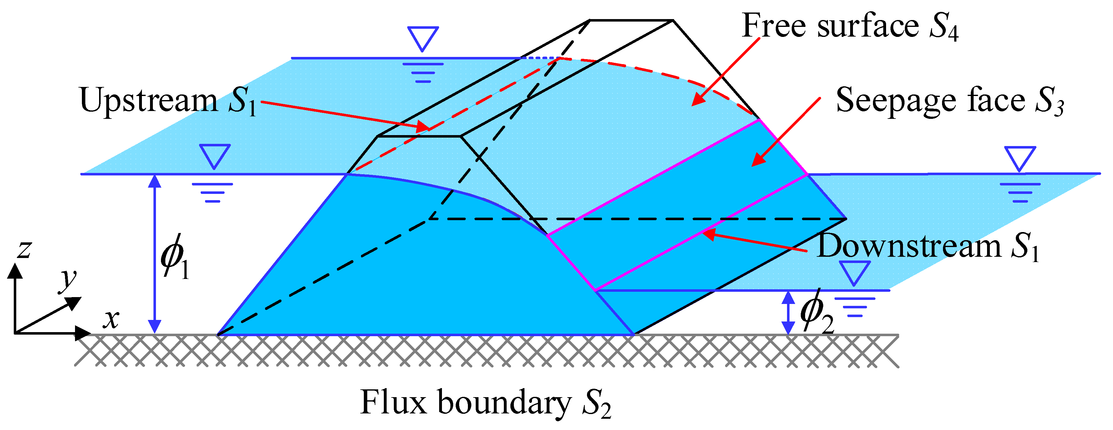
For steady free surface flow through a three-dimensional soil dam, as plotted in Figure 1, subsurface flow is promoted by the upstream and downstream head difference, and a free surface exists between the wet domain and dry domain. When the porous media, involving grains and pores, is supposed as a continuum, the three-dimensional seepage flow through the wet domain is governed by:

$$\frac{\partial v_x}{\partial x}+\frac{\partial v_y}{\partial y}+\frac{\partial v_z}{\partial z}=0$$

(1)

where x, y and z are three coordinate axes in the Cartesian system; v_x, v_y and v_z denote the flow velocity in the x, y and z (or 1, 2 and 3) directions, respectively:

$$\{\begin{array}{l}{v}_x=-k_x\partial \varphi /\partial x\\ v_y=-k_y\partial \varphi /\partial y\\ v_z=-k_z\partial \varphi /\partial z\end{array}$$

(2)

where k_x, k_y and k_z denote the saturated hydraulic conductivity in the x, y and z (or 1, 2 and 3) directions, respectively; $\varphi =p/(\rho g)+z$ is the total head of water; and $p/(\rho g)$ is the water pressure head.

The boundary conditions subject to Equation (1) yield:

$$\varphi =\overline{\varphi } \mathrm{on} S_1$$

(3)

$$q_n=-\left(v_x{n}_x+v_y{n}_y+v_z{n}_z\right)=0 \mathrm{on} S_2$$

(4)

$$\varphi =z; q_n\le 0 \mathrm{on} S_3$$

(5)

$$\varphi =z; q_n=0 \mathrm{on} S_4$$

(6)

where the overline represents a given value, n denotes the unit normal vector; q is the flow flux; and S₁, S₂, S₃ and S₄ are the water head, flux, seepage face and free surface boundaries, respectively.

2.2. Equivalent Flow Velocity, Hydraulic Conductivity and Continuity Equation

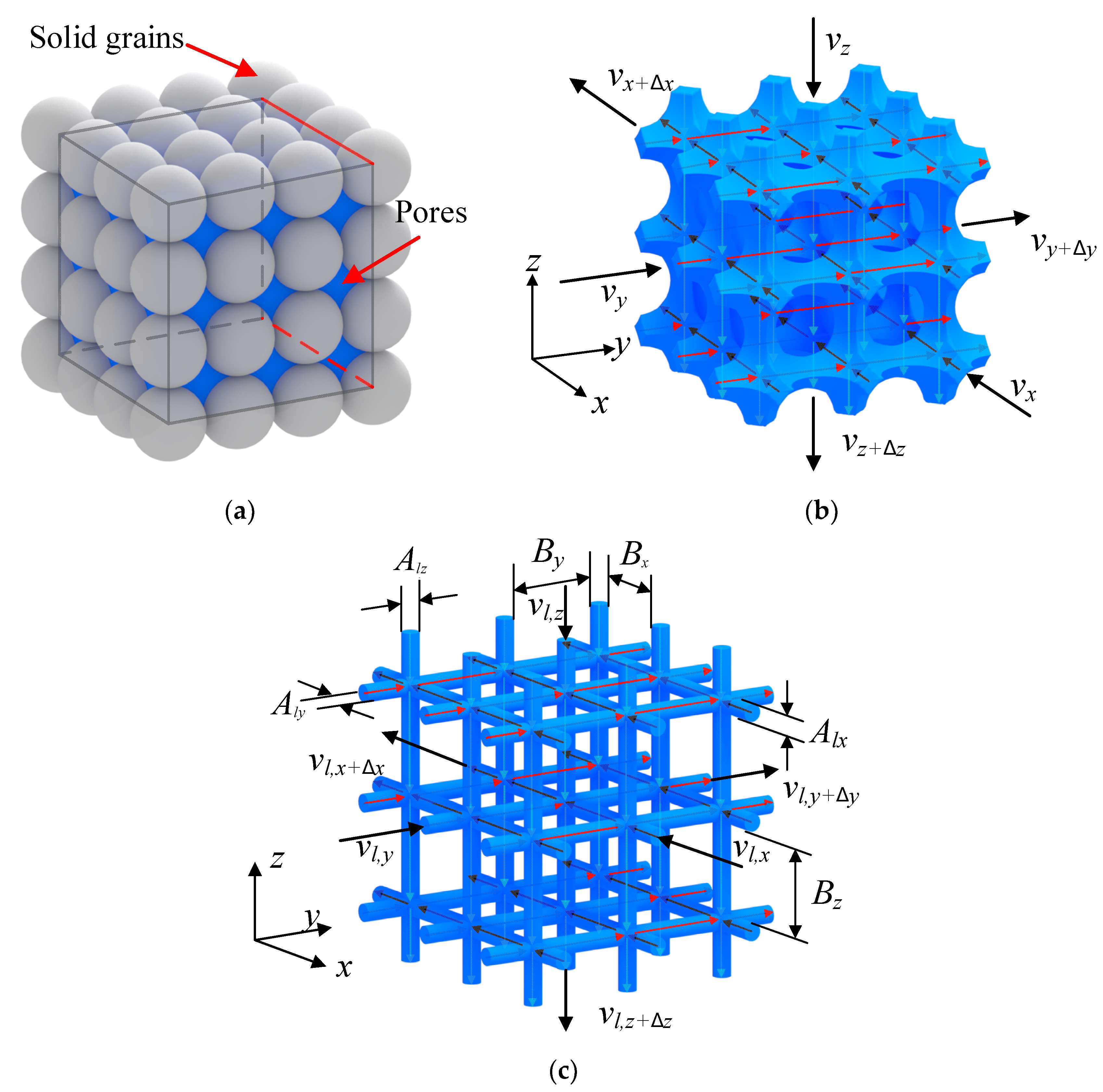
Based on the concept of representative elementary volume, a hypothetical continuum is frequently applied to describe the hydraulic behavior in porous media, and water flow is homogenized to the whole control volume. Considering the fact that water flow can only occur through the pores between solid grains, two-dimensional homogeneous porous media have been simulated by a pipe network model proposed by Xu et al. [13], Ren et al. [15], Afzali and Monadjemi [14], Abareshi et al. [16], Moosavian [17], Ye et al. [12,18,19] and Wei et al. [20]. In order to extend the two-dimensional pipe network model to three-dimensional porous media for free surface flow analysis, a typical ordered porous medium with cubic packing of uniform spherical grains (grey color) is shown in Figure 2a; the void space between spherical grains for water permeating in the x, y and z directions can be generalized as a three-dimensional orthogonal line network, as shown in Figure 2b,c.

When the line elements in the x direction are specified with a hydraulic conductivity k_lx and a cross-section area A_lx, the flow velocity v_lx and flow rate Q_x through the line elements in the x direction can also be described by Darcy’s law:

$$v_{lx}=k_{lx}\frac{\partial \varphi }{\partial x}$$

(7)

$$Q_x=v_{lx}·A_{lx}{N}_y{N}_z=k_{lx}\frac{\partial \varphi }{\partial x}·A_{lx}{N}_y{N}_z$$

(8)

where N_y and N_z are the number of rows and columns of the x-directional line elements in the control volume.

For the homogeneous continuum model, the x-directional flow rate yields:

$$Q_x=v_{x}dx=k_x\frac{\partial \varphi }{\partial x}\Delta y\Delta z$$

(9)

where Δy and Δz are the width and height of the control volume.

In order to obtain a consistent numerical solution based on the line-element model, the flow rate through the control volume should be balanced, and the equality of Equations (8) and (9) gives:

$$k_{lx}=\frac{k_x}{A_{lx}}\frac{\Delta y}{N_y}\frac{\Delta z}{N_z}=\frac{k_x}{A_{lx}}{B}_y{B}_z$$

(10)

where B_y and B_z are the row and column distances, as shown in Figure 2c, and are equal to Δy/N_y and Δz/N_z, respectively. For convenience, in mathematics, A_ij is nominated as a unit of area, and Equation (10) is reduced to:

$$k_{lx}=k_x{B}_y{B}_z$$

(11)

Similarly, the equivalent flow velocity v_ly, v_lz and hydraulic conductivity k_ly, k_lz can be derived as:

$$v_{ly}=k_{ly}\frac{\partial \varphi }{\partial y}$$

(12)

$$k_{ly}=k_y{B}_x{B}_z$$

(13)

$$v_{lz}=k_{lz}\frac{\partial \varphi }{\partial z}$$

(14)

$$k_{lz}=k_z{B}_x{B}_y$$

(15)

where B_x is the x-directional distance.

In the line-element model, the flow velocity is parallel to the line elements, and there is no vertical component, such as v_ly = v_lz = 0 in the x-directional line elements. Thus, the continuity Equation (1) in the x, y and z directions can be simplified as:

$$\frac{\partial v_{lx}}{\partial x}=\frac{\partial }{\partial x}\left(k_{lx}\frac{\partial \varphi }{\partial x}\right)=0$$

(16)

$$\frac{\partial v_{ly}}{\partial y}=\frac{\partial }{\partial y}\left(k_{ly}\frac{\partial \varphi }{\partial y}\right)=0$$

(17)

$$\frac{\partial v_{lz}}{\partial z}=\frac{\partial }{\partial z}\left(k_{lz}\frac{\partial \varphi }{\partial z}\right)=0$$

(18)

2.3. Unified Formulations and Boundary Conditions

Instead of the Cartesian coordinate system, a local coordinate system l is assigned to each line element. Therefore, the flow velocity in the x, y and z directions can be unified as:

$$v_{ij}=k_{ij}\frac{\partial \varphi }{\partial l}$$

(19)

where i and j are the two endpoints of the line element.

In general, free surface flow problems are solved based on the fixed-mesh method, and Darcy’s law for saturated flow is extended to the whole flow domain, including the dry area. Following Zheng et al. [10] and Ye et al. [12], a continuous penalized Heaviside function $H_{\lambda }\left(\varphi -z\right)$ is employed to generalize the seepage flow through wet and dry areas:

$$v_{ij}=H_{\lambda }\left(\varphi -z\right)k_{ij}\frac{\partial \varphi }{\partial l}$$

(20)

$$H_{\lambda }\left(\varphi -z\right)=\{\begin{array}{ll}1& \mathrm{if} \varphi -z\ge 0 \\ \left(\lambda +\varphi -z\right)/\lambda & \mathrm{if} 0>\varphi -z>-\lambda \\ 0& \mathrm{if} \varphi -z\le -\lambda \end{array}$$

(21)

where λ is a penalty parameter to describe the transition thickness from the wet area to the entirely dry area.

By combining Equation (20), the unified continuity equation from Equations (16)–(18) can be stated as:

$$\frac{\partial }{\partial l}\left[H_{\lambda }\left(\varphi -z\right)k_{ij}\frac{\partial \varphi }{\partial l}\right]=0$$

(22)

The equivalent boundary conditions are expressed as:

$${\varphi }_i={\overline{\varphi }}_i \mathrm{on} S_1$$

(23)

$$q_i=0 \mathrm{on} S_2$$

(24)

$${\varphi }_i=z_i; q_i\le 0 \mathrm{on} S_3$$

(25)

$${\varphi }_i=z_i; q_i=0 \mathrm{on} S_4$$

(26)

3. Finite Line-Element Method

From Equations (20)–(26), it can be seen that the three-dimensional steady free surface flow can be simplified into one-dimensional form based on the line-element model. Thus, the functional I($\varphi$) of Equation (22) can be derived based on the one-dimensional line element:

$$I\left(\varphi \right)={\displaystyle \sum _{\mathrm{\Omega }}{\displaystyle {\int }_{l_{ij}}\frac{1}{2}{H}_{\lambda }\left(\varphi -z\right)k_{ij}{\left(\frac{\partial \varphi }{\partial l}\right)}^{2}dl}}$$

(27)

where Ω is the entire flow domain, including wet and dry areas.

Minimizing the functional I($\varphi$) yields:

$$\frac{\partial I}{\partial {\varphi }_i}={\displaystyle \sum _{\mathrm{\Omega }}{\displaystyle {\int }_{l_{ij}}{H}_{\lambda }\left(\varphi -z\right)k_{ij}\frac{\partial \varphi }{\partial l}\frac{\partial }{\partial {\varphi }_i}\left(\frac{\partial \varphi }{\partial l}\right)dl}}=0$$

(28)

When the linear interpolation method is applied to quantify the water head and coordinate functions of each line element, the matrix form for Equation (28) can be expressed as:

$$\mathit{K}{\mathit{h}}^{\eta +1}=\mathit{q}$$

(29)

in which

$$\mathit{K}={\displaystyle \sum _{\mathrm{\Omega }}{\displaystyle {\int }_{l_{ij}}{\mathit{B}}^{\mathrm{T}}{k}_{ij}\mathit{B}dl}}$$

(30)

$$\mathit{q}={\displaystyle \sum _{\mathrm{\Omega }}{\displaystyle {\int }_{l_{ij}}\left(1-H_{\lambda }\right){\mathit{B}}^{\mathrm{T}}{k}_{ij}\mathit{B}dl}}·{\mathit{\varphi }}^{\eta }$$

(31)

$$\mathit{B}=\left[\begin{array}{cc}-1/l_{ij}& 1/l_{ij}\end{array}\right]$$

(32)

where B is the one-dimensional geometric matrix in the local coordinate system, and η is the iteration step. The iterative process should satisfy the convergence condition as below:

$$\Vert {\mathit{\varphi }}^{\eta +1}-{\mathit{\varphi }}^{\eta }\Vert \le \delta \Vert {\mathit{\varphi }}^{\eta }\Vert$$

(33)

where δ is the error tolerance.

4. Validations

4.1. A Rectangular Dam with Tailwater

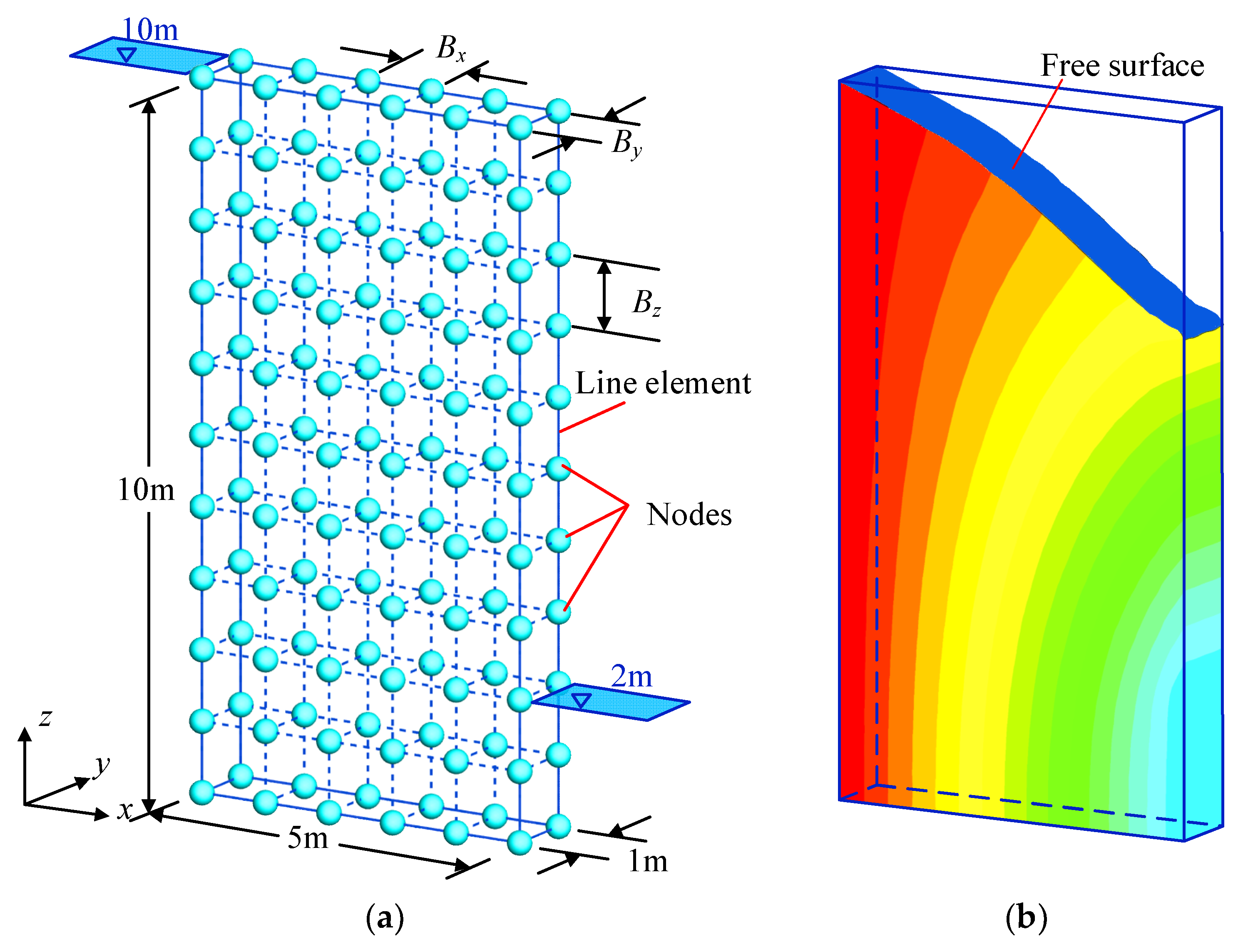
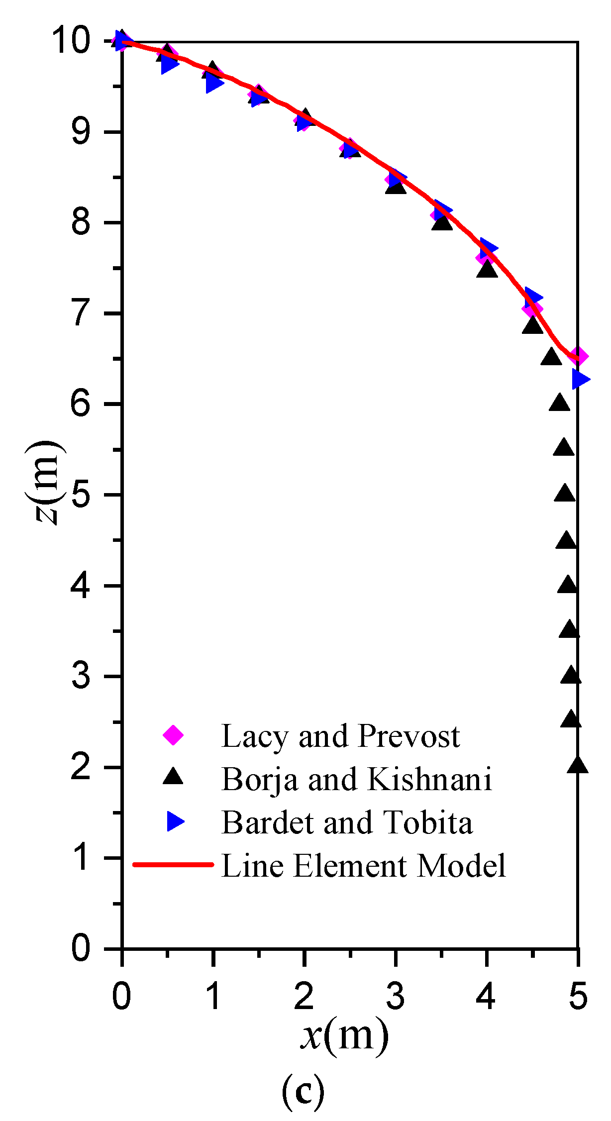
The classical numerical solution for steady free surface flow in a homogeneous rectangular dam from Lacy and Prevost [8] is employed to validate the proposed method. The size and flow condition are shown in Figure 3a, and the hydraulic conductivity is 1 m/d. At first, the flow domain is meshed into three orthogonal sets of line elements with B_x = B_y = B_z = 0.1 m, and the penalty parameter λ is valued as 1 × 10⁻¹⁰. The water head distribution and free surface locations are shown in Figure 3b,c, respectively. For comparison, the numerical predictions from Borja and Kishnani [9] and Bardet and Tobita [21] are also plotted. The results from Borja and Kishnani have a considerable discrepancy near the downstream because of singular seepage points. The free surface predicted by the proposed line-element method agrees well with that from Lacy and Prevost and Bardet and Tobita.

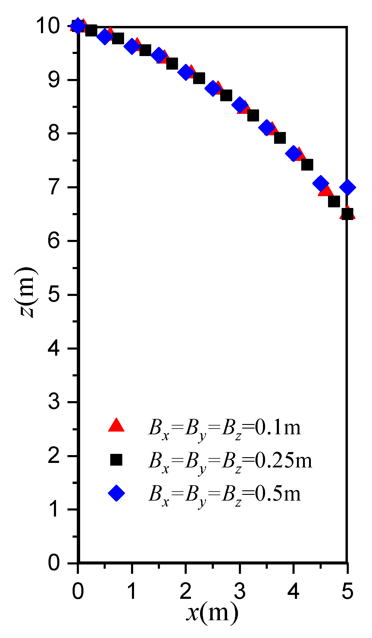
In order to investigate the dependency of mesh sizes and penalty parameters on free surface location, numerical efficiency and flow rate, seepage analysis with different mesh sizes (B_x = B_y = B_z = 0.1 m, 0.25 m, 0.5 m) and penalty parameters (λ = 1 × 10⁻¹⁰, 0.01, 0.1, 0.25, 0.5) are considered. The free surface locations from different mesh sizes are plotted in Figure 4; the three curves are almost identical except that the seepage point from B_x = B_y = B_z = 0.5 m is higher than others. As a result, the influence of mesh size is not notable on the distribution of free surface but on seepage point.

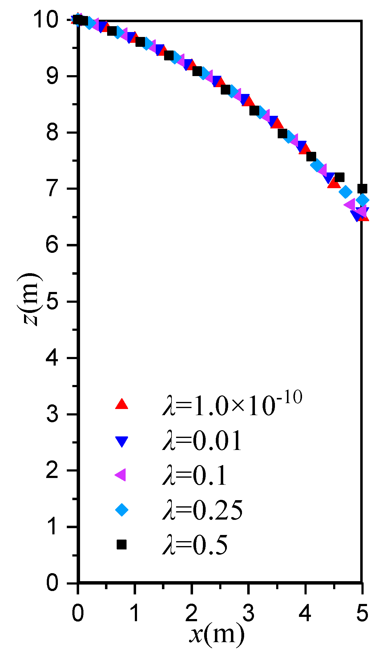
The effect of the penalty parameter λ on free surface locations is shown in Figure 5. With decreasing λ, the free surface becomes steeper, and the seepage point becomes lower. The discharges per unit width, iteration step and relative error are listed in

Table 1. The discharge per unit width, iteration step and relative error.

λ	Analytical (m2/s)	Numerical (m2/s)	Iteration Steps	Relative Error
1 × 10−10	1.111 × 10−4	1.100 × 10−4	8	0.99
0.01		1.100 × 10−4	8	0.99
0.10		1.100 × 10−4	8	0.99
0.25		1.099 × 10−4	8	1.08
0.50		1.092 × 10−4	7	1.71

. Based on Dupuit’s formula $q=k\left({\varphi }_1^2-{\varphi }_2^2\right)/2L$ [22], where ${\varphi }_1$ and ${\varphi }_2$ are the upstream and downstream water heads and L is the dam length as 5 m, the analytical discharge per unit width is equal to 1.111 × 10⁻⁴ m²/s. The relative error between the numerical and analytical results decreases with the decrease in λ. It is found that when λ is equal to or less than 0.1, the calculated free surface location, discharge per unit width and iteration step is independent of λ. Therefore, λ = 0.1 is used for other illustrated examples. Note that the error tolerance is set as 0.001, which can guarantee numerical accuracy and efficiency.

4.2. A right Trapezoidal Dam

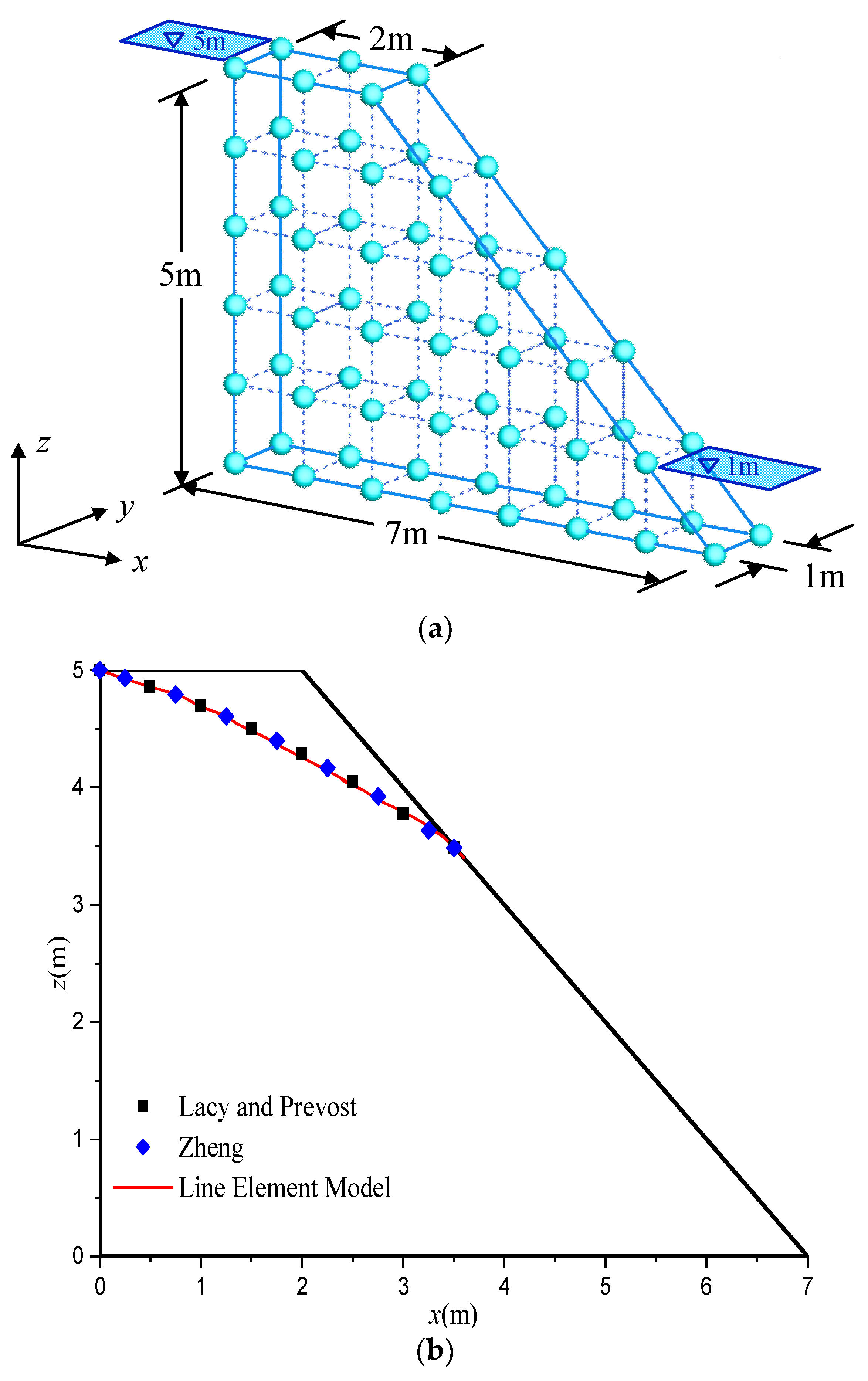
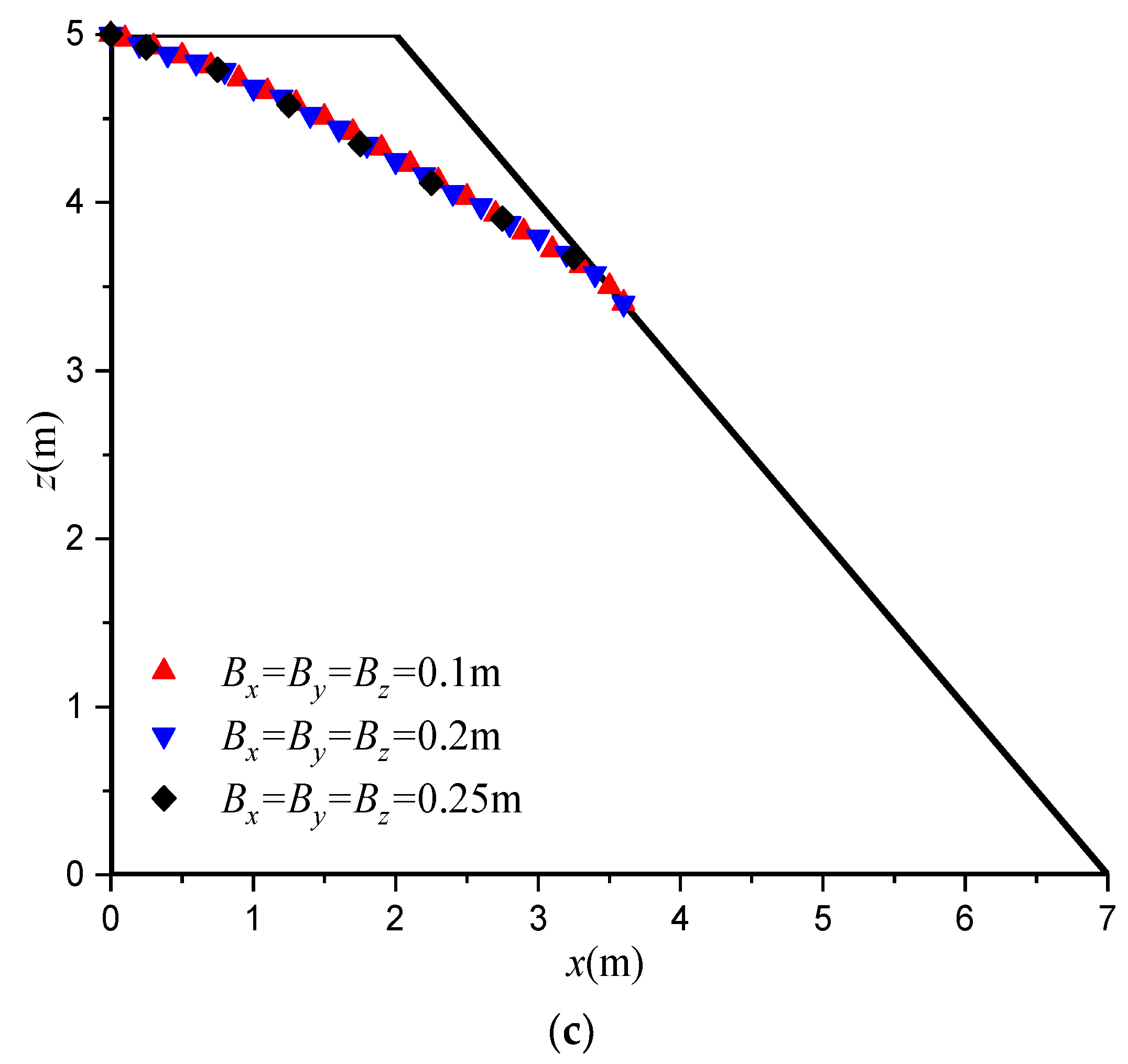
As shown in Figure 6a, the size of a right trapezoidal dam is 7 m in length, 5 m in height and 1 m in width. The upstream and downstream water heads are 5 m and 1 m, respectively. The bottom boundary is impermeable. The dam is isotropic, and the hydraulic conductivity is valued as 1 m/d. During numerical simulations, the dam is discretized by three kinds of mesh size (B_x = B_y = B_z = 0.1 m, 0.2 m, 0.25 m), and the related predictions of free surface are shown in Figure 6c. In addition, the finite element results based on the continuum model from Lacy and Prevost [8] and Zheng et al. [10] are also presented in Figure 6b for comparison. There is good agreement between the proposed line-element approach and the continuum-based finite element methods. In this right trapezoidal dam, the proposed line-element model is also not sensitive to the mesh size and can achieve an accurate solution in six iterations.

4.3. A Left Bank Abutment Slope of Kajiwa Dam in Southwestern China

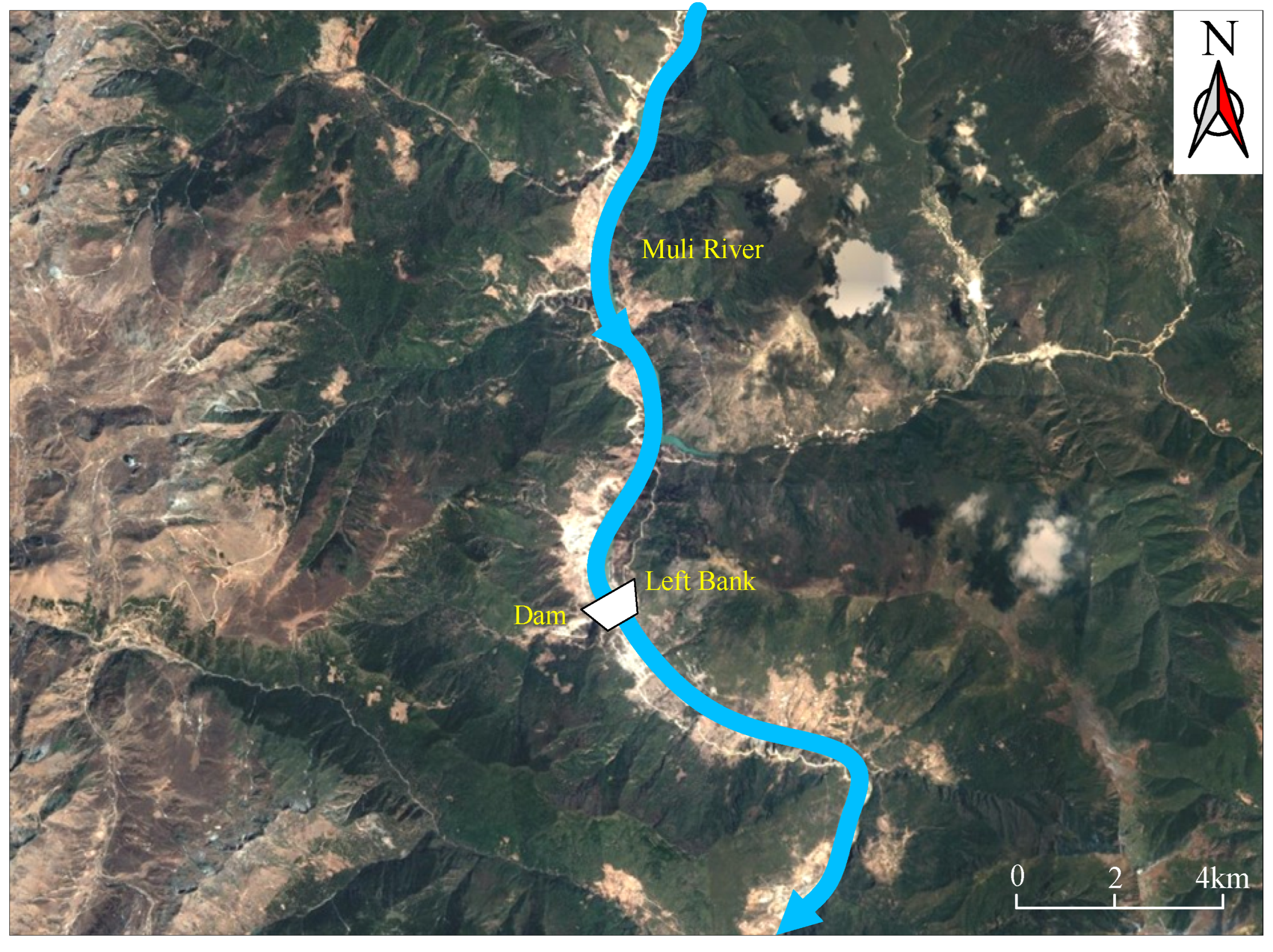
Located in the upper reaches of the Muli River in Muli County, Sichuan Province, as shown in Figure 7, Kajiwa Hydropower Station is about 178 km away from Muli County and 424 km away from Xichang City, which controls a watershed area of 6598 km² with an annual average flow of 101 m³/s. This concrete face rockfill dam is 171 m in height, and the crest elevation is 2885 m. The installed capacity is 452.4 MW, and the total storage capacity is 374.5 million m³ at the normal water level of 2850 m.

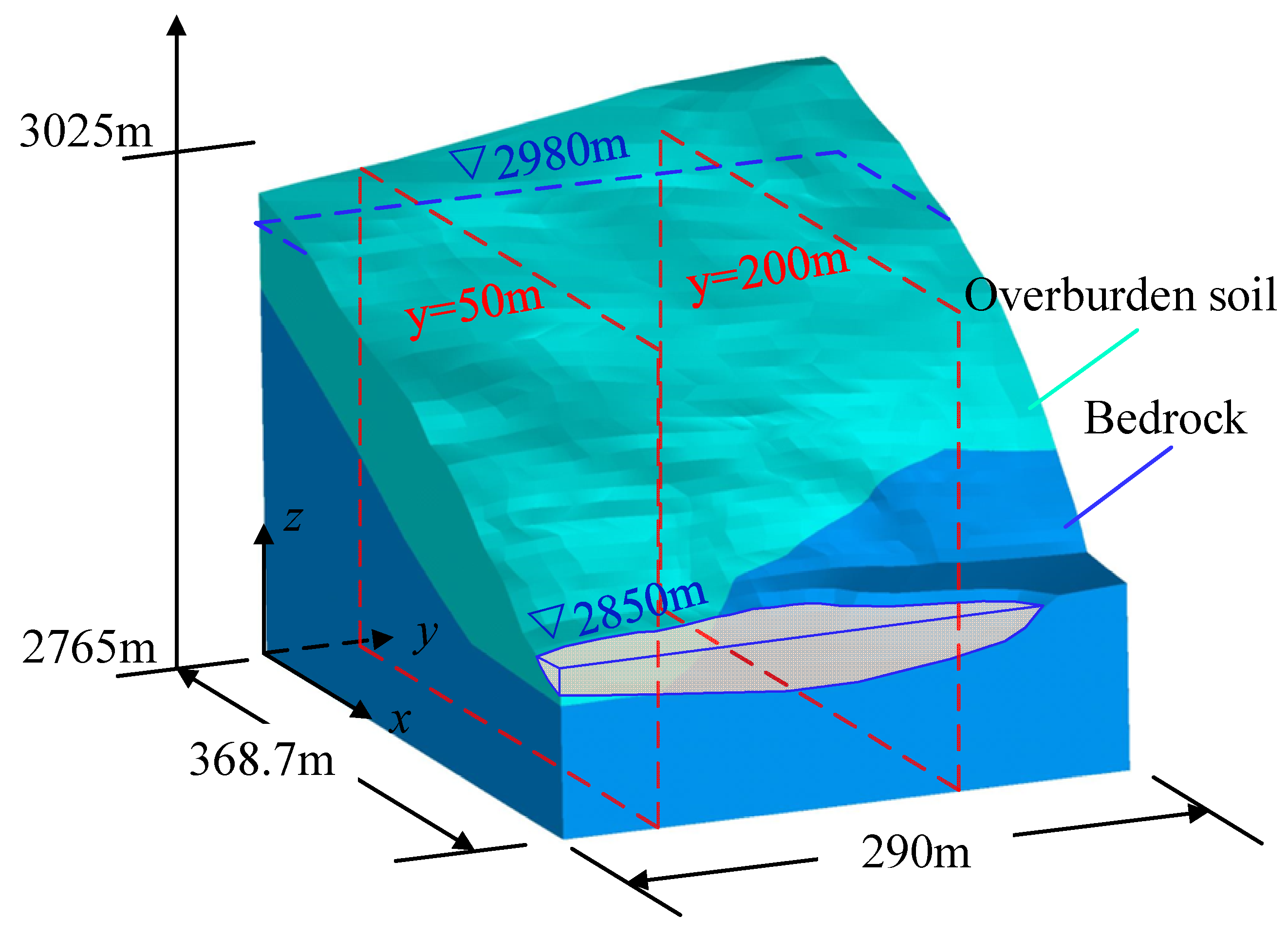
The dam site is located in a deep and slightly asymmetrical V-shaped valley, with exposed bedrock on both the right and left banks and steep partial terrain. The left bank is broken-line-type with a slope of about 50° between 2710 m and 2830 m, a slope of about 30° between 2830 m and 2970 m, and there are multistage wide and gentle platforms with slopes of 10~15° above 2970 m, as shown in Figure 8. Between 2710 m and 2830 m, a small amount of landslide deposits have accumulated at the foot of the slope, and the residual exposed bedrock consists of slate and phyllitic slate intercalated sandstone from the third member (O₁r³) and metamorphic quartz sandstone, carbonaceous slate and phyllitic slate from the fourth member (O₁r⁴) of the Rengong Formation of the lower Ordovician system. Above 2830 m, the slope surface is covered by a large area of residual slope deposits and mainly consists of the glacial fluvial (fglQ3), eluvial (el plus dlQ4), colluvial (col plus dlQ4) and diluvial (plQ4) deposits.

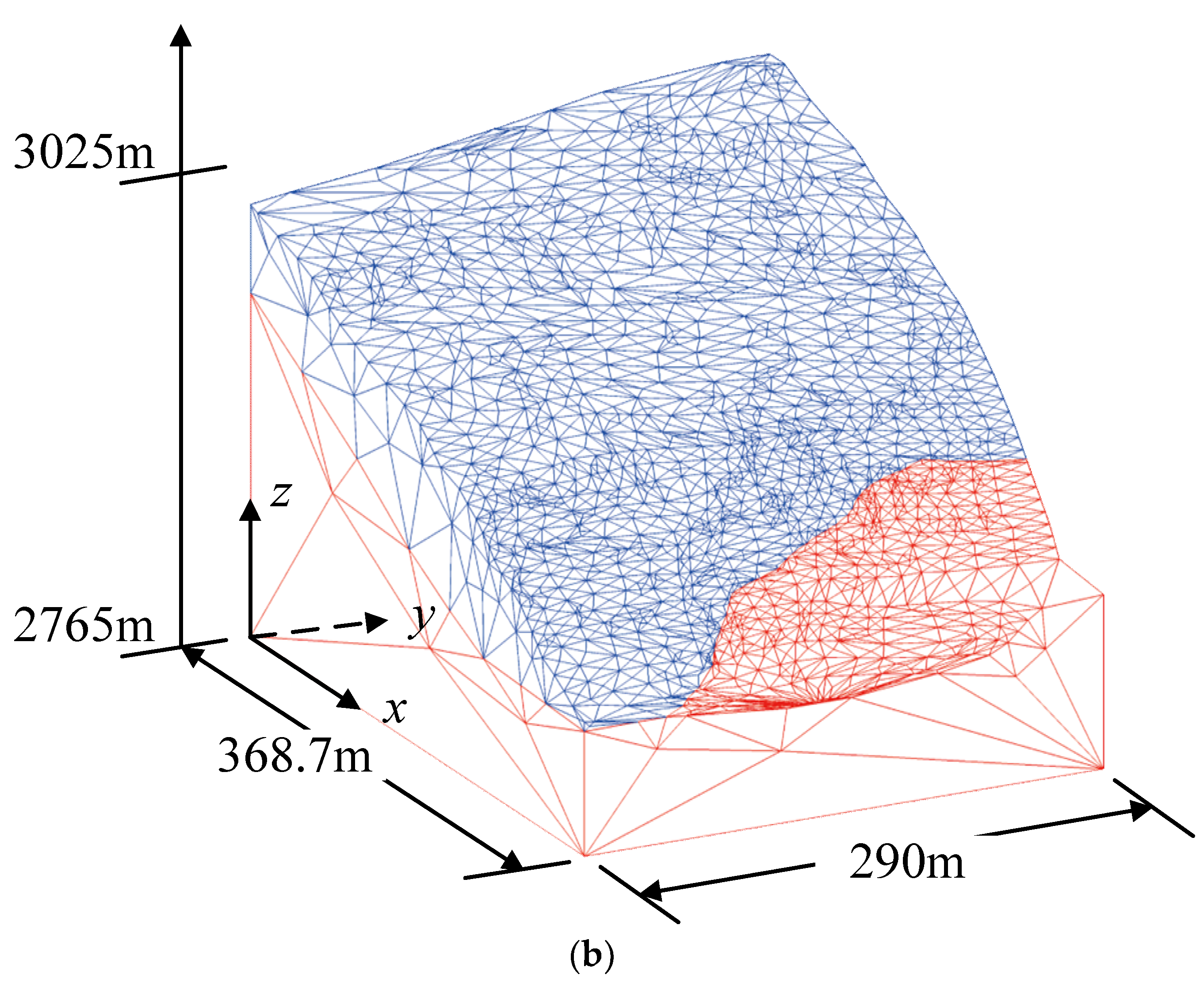
The left bank abutment slope is close to important hydraulic structures such as the entrance of the no. 1 spillway tunnel, the entrance of the emptying tunnel and the left dam abutment; the influence of seepage flow on its stability has an important impact on the construction and permanent operation safety of the Kajiwa Hydropower Station. In order to investigate the seepage flow behavior around the left bank abutment, the size of the whole flow domain is 290 m along the river flow direction, 368.7 m perpendicular to the river flow direction and 260 m in height, as shown in Figure 8. The geological strata are simplified as two layers: overburden soil and bedrock, of which the permeabilities are 6.43 × 10⁻⁶ m/s and 1.5 × 10⁻¹⁰ m/s, respectively. The water level along the mountain side is 2980 m, and along the river side, it is 2850 m. The bottom and lateral boundaries perpendicular to the river are impermeable, and the residual boundary is specified as a potential seepage boundary.

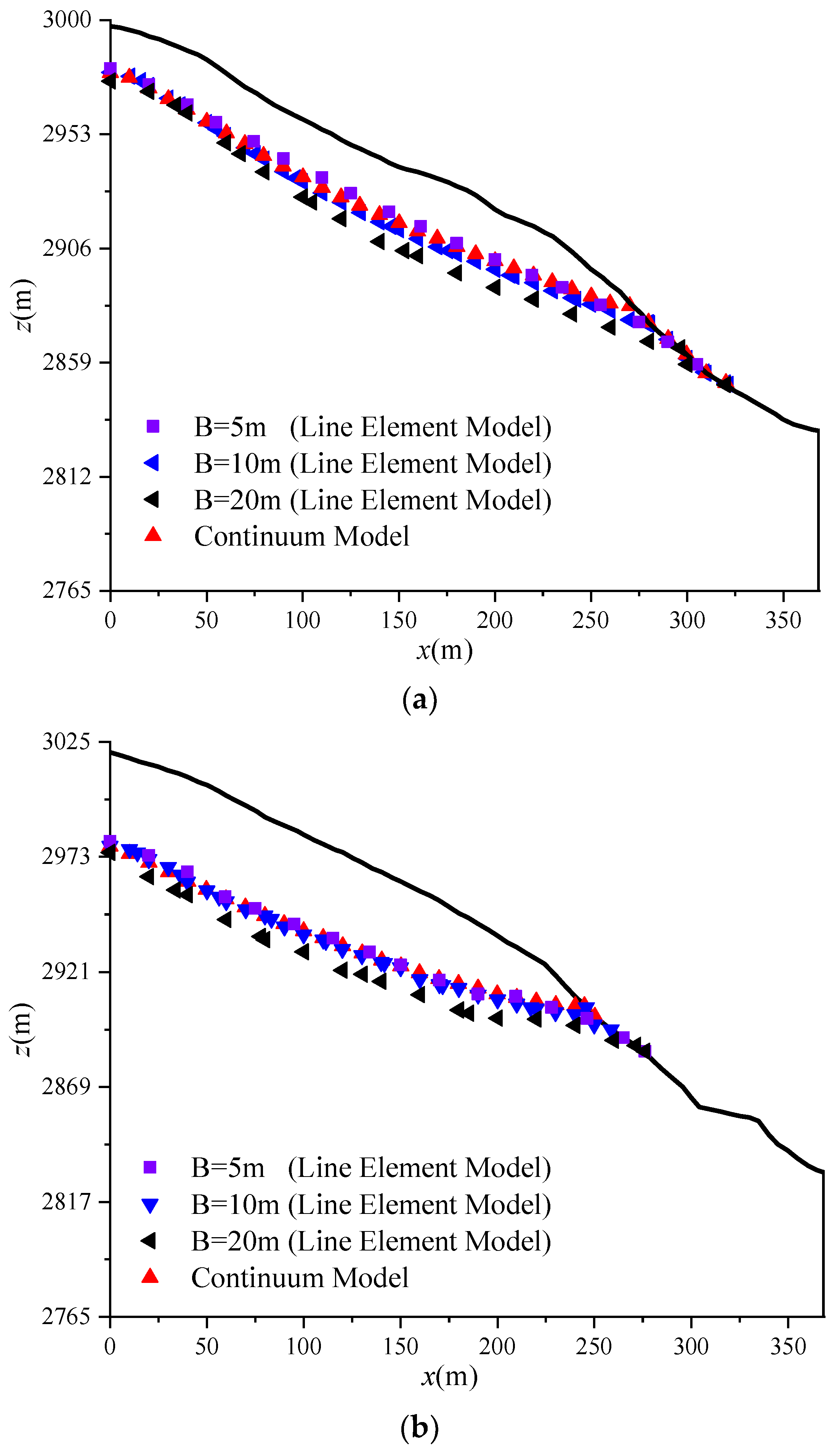
Based on the line-element model, the left bank abutment slope is discretized by three kinds of mesh size (B_x = B_y = B_z = 5 m, 10 m, 20 m). As shown in Figure 9, by comparing the three kinds of mesh size, it can be seen that the results from B_x = B_y = B_z = 5 m and B_x = B_y = B_z = 10 m are almost overlapped and agree well with the continuum model. In contrast, the deviation of B_x = B_y = B_z = 20 m is pronounced. In order to obtain higher calculation accuracy and consume less calculation time, the mesh size of B_x = B_y = B_z = 10 m is selected in this paper.

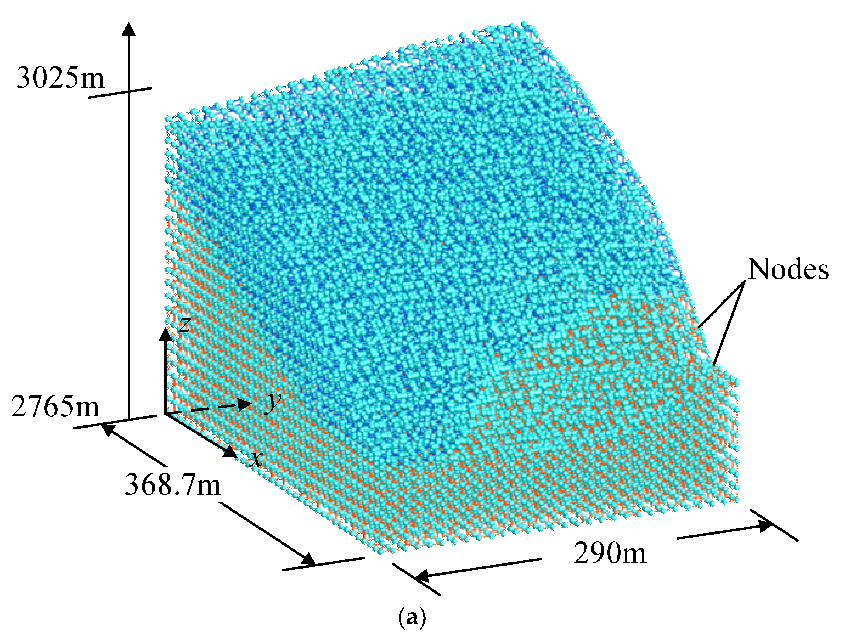
During numerical simulations, the left bank abutment slope is meshed by three orthogonal sets of line elements with B_x = B_y = B_z = 10 m, as shown in Figure 10a, with line elements and nodes. For comparison, the tetrahedron element mesh (Figure 10b) is also presented to model the three-dimensional steady free surface flow based on the parabolic variational inequality algorithm of Signorini’s condition proposed by Zheng et al. [10] and Chen et al. [1], and the details are as follows:

By combining with Equation (21), the continuum-based finite-element matrix for Equation (1) can be expressed as [1]:

$$\mathit{K}{\mathit{\varphi }}^{r+1}={\mathit{q}}^r$$

(34)

in which

$$\mathit{K}={\displaystyle \sum _e{\displaystyle {\int }_{{\mathrm{\Omega }}_e}{\mathit{B}}^T\mathit{k}\mathit{B}dxdydz}}$$

(35)

$${\mathit{q}}^r={\displaystyle \sum _e{\displaystyle {\int }_{{\mathrm{\Omega }}_e}\left[1-H\left(\varphi -z\right)\right]{\mathit{B}}^T\mathit{k}\mathit{B}dxdydz·}}{\mathit{\varphi }}^r$$

(36)

$$\mathit{B}=\left[\begin{array}{ccc}\frac{\partial N_1}{\partial x}& \frac{\partial N_2}{\partial x}& \begin{array}{cc}\cdots & \frac{\partial N_m}{\partial x}\end{array}\\ \frac{\partial N_1}{\partial y}& \frac{\partial N_2}{\partial y}& \begin{array}{cc}\cdots & \frac{\partial N_m}{\partial y}\end{array}\\ \frac{\partial N_1}{\partial z}& \frac{\partial N_2}{\partial z}& \begin{array}{cc}\cdots & \frac{\partial N_m}{\partial z}\end{array}\end{array}\right]$$

(37)

$$\mathit{N}=\left[\begin{array}{cccc}{N}_1& N_2& \cdots & N_m\end{array}\right]$$

(38)

where B is the partial derivatives matrix of N, N_i is the shape function and m is the node number of volume element.

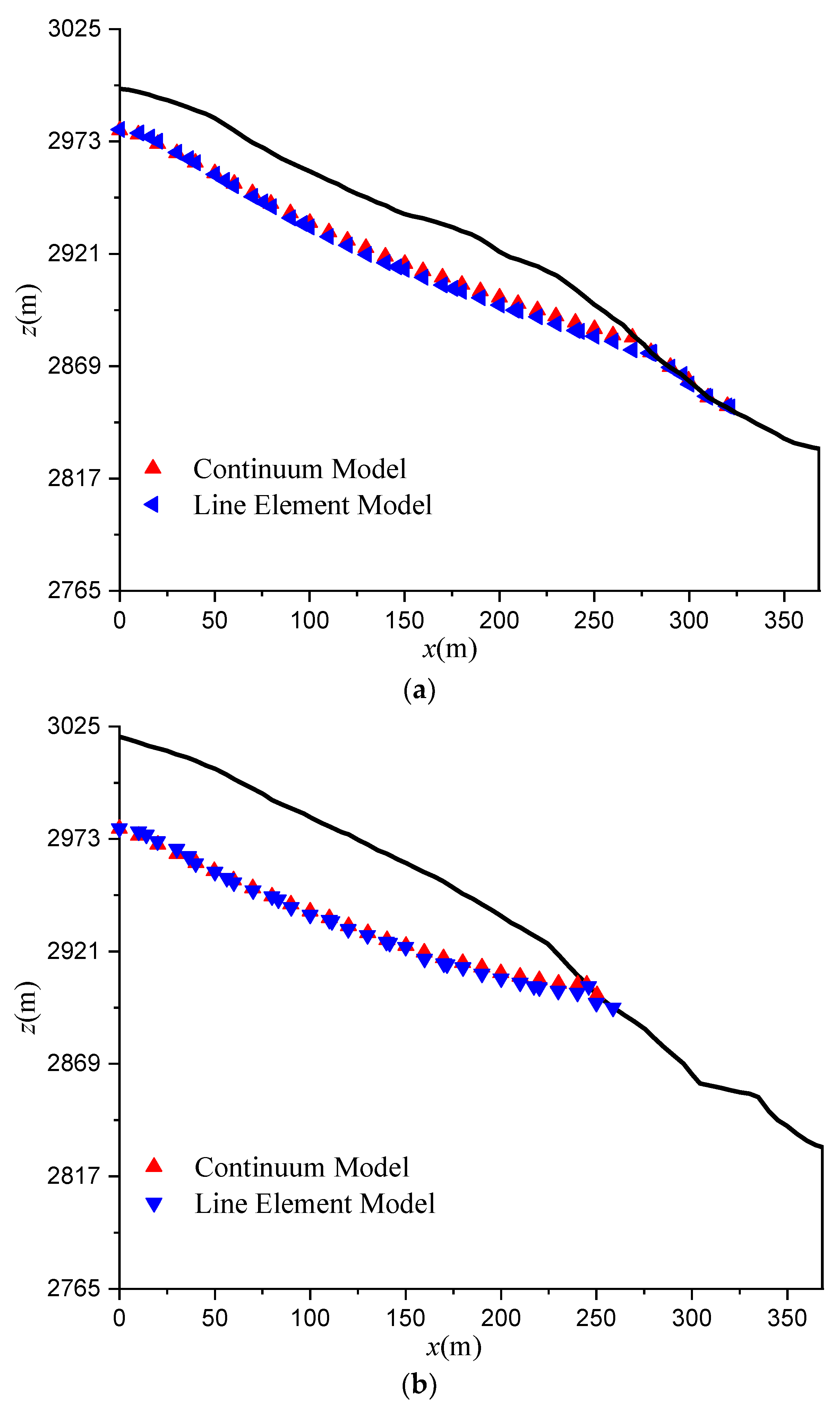
The contours of the three-dimensional water pressure head between the proposed line-element model and the parabolic variational inequality algorithm are shown in Figure 11, and good agreement is obtained. Figure 12 also plots the free surface locations in the profiles y = 50 m and 200 m. The calculated results from these two methods are very close, which indicates that the proposed line-element model can well reproduce the numerical predictions from the continuum-based method. For this three-dimensional seepage condition, the seepage point at the profile y = 200 m is higher than that at the profile y = 50 m; this is because the exposed bedrock with weak permeability at the bottom of y = 200 m is negative for water transportation. It should be noted that the numerical solution is achieved at six iteration steps, indicating that the proposed line-element approach is feasible and efficient for solving complicated engineering seepage problems.

5. Conclusions

For three-dimensional steady free surface flow in porous media, a line-element model was developed to characterize water flow through the pores between the solid grains in the control volume. Instead of the hypothesis that water flow is homogenized to the whole flow domain, including pores and solid grains, the pores in the x, y and z directions in the control volume are conceptualized as a three-dimensional orthogonal network of line elements. Considering the equivalent distributions of water head and flow balance between the line-element model and continuum model, the equivalent flow velocities, hydraulic conductivities and continuity equations in the x, y and z directions are derived.

In order to assess the steady free surface flow in a fixed domain, a continuous penalized Heaviside function is employed to extend the saturated Darcy flow to the unsaturated flow including the dry domain. Based on the local coordinate system, the equivalent flow velocities and continuity equations in the x, y and z directions are unified in a one-dimensional form, and the finite line-element algorithm is established by minimizing the functional of the continuity equation. Herein, three-dimensional steady free surface flow is reduced to one-dimensional form, and the numerical procedure is highly simplified, such as the geometric matrix only depends on the length of the line element, while that of the continuum model is a function of the coordinates of x, y and z; the integral calculation of K in the line-element model is accurate, while that of the continuum model is approximate subject to Gaussian points. Therefore, the proposed line-element model can obtain accurate solutions in a few steps, especially for complicated engineering applications, and the numerical difficulty is greatly decreased.

During the comparisons with other methods for three-dimensional steady free surface flow in a rectangular dam and a right trapezoidal dam, the numerical accuracy and efficiency can be well guaranteed by the line-element model. The line-element model is not highly sensitive to mesh size and penalty parameters, but large mesh sizes and penalty parameters may lead to variation in seepage points and free surface distributions around the seepage face.

From the application of the left bank abutment slope of the Kajiwa Dam in Southwestern China, the heterogeneous slope generally contains two kinds of geological layers: the overburden soil and bedrock, with several orders of hydraulic conductivity difference, which arises through seepage points around the exposed bedrock domain that are higher than those near the landslide deposits at the foot of the slope. At the same time, the numerical results from the parabolic variational inequality algorithm are also provided, in which the slope is meshed by the tetrahedron elements. The three-dimensional contours of the water pressure head and free surface locations of the profiles between the line-element model and continuum model are almost consistent. Therefore, the line-element model is equivalent to the continuum model in numerical solutions. However, the line model seems to be more reasonable in physics, more concise in mathematics and easier in solutions.

References

- Chen, Y.; Zhou, C.; Zheng, H. A numerical solution to seepage problems with complex drainage systems. Comput. Geotech. 2008, 35, 383–393. [Google Scholar] [CrossRef]
- Chen, Y.F.; Ye, Y.; Hu, R.; Yang, Z.; Zhou, C.B. Modeling unsaturated flow in fractured rocks with scaling relationships between hydraulic parameters. J. Rock Mech. Geotech. Eng. 2022, 14, 1697–1709. [Google Scholar] [CrossRef]
- Zhou, C.; Chen, Y.; Jiang, Q.; Lu, W. A generalized multi-field coupling approach and its application to stability and deformation control of a high slope. J. Rock Mech. Geotech. Eng. 2011, 3, 193–206. [Google Scholar] [CrossRef] [Green Version]
- Jiang, Q.; Qi, Z.; Wei, W.; Zhou, C. Stability assessment of a high rock slope by strength reduction finite element method. Bull. Eng. Geol. Environ. 2015, 74, 1153–1162. [Google Scholar] [CrossRef]
- Li, Y.; Chen, Y.F.; Zhang, G.J.; Liu, Y.; Zhou, C.B. A numerical procedure for modeling the seepage field of water-sealed underground oil and gas storage caverns. Tunn. Undergr. Space Technol. 2017, 66, 56–63. [Google Scholar] [CrossRef]
- Bathe, K.; Khoshgoftaar, M. Finite element free surface seepage analysis without mesh iteration. Int. J. Numer. Anal. Methods Geomech. 1979, 3, 13–22. [Google Scholar] [CrossRef] [Green Version]
- Desai, C.S.; Li, G.C. A residual flow procedure and application for free surface flow in porous media. Adv. Water Resour. 1983, 6, 27–35. [Google Scholar] [CrossRef]
- Lacy, S.J.; Prevost, J.H. Flow through porous media: A procedure for locating the free surface. Int. J. Numer. Anal. Methods Geomech. 1987, 11, 585–601. [Google Scholar] [CrossRef]
- Borja, R.I.; Kishnani, S.S. On the solution of elliptic free-boundary problems via Newton’s method. Comput. Methods Appl. Mech. Eng. 1991, 88, 341–361. [Google Scholar] [CrossRef]
- Zheng, H.; Liu, D.; Lee, C.; Tham, L. A new formulation of Signorini’s type for seepage problems with free surfaces. Int. J. Numer. Methods Eng. 2005, 64, 1–16. [Google Scholar] [CrossRef]
- Wang, Y.; Hu, M.; Zhou, Q.; Rutqvist, J. A new second-order numerical manifold method model with an efficient scheme for analyzing free surface flow with inner drains. Appl. Math. Model. 2016, 40, 1427–1445. [Google Scholar] [CrossRef]
- Ye, Z.; Qin, H.; Chen, Y.; Fan, Q. An equivalent pipe network model for free surface flow in porous media. Appl. Math. Model. 2020, 87, 389–403. [Google Scholar] [CrossRef]
- Xu, Z.H.; Ma, G.W.; Li, S.C. A graph-theoretic pipe network method for water flow simulation in a porous medium: GPNM. Int. J. Heat Fluid Flow 2014, 45, 81–97. [Google Scholar] [CrossRef]
- Afzali, S.H.; Monadjemi, P. Simulation of flow in porous media: An experimental and modeling study. J. Porous Media 2014, 17, 469–481. [Google Scholar] [CrossRef]
- Ren, F.; Ma, G.; Wang, Y.; Fan, L. Pipe network model for unconfined seepage analysis in fractured rock masses. Int. J. Rock Mech. Min. Sci. 2016, 88, 183–196. [Google Scholar] [CrossRef]
- Abareshi, M.; Hosseini, S.M.; Sani, A.A. Equivalent pipe network model for a coarse porous media and its application to two-dimensional analysis of flow through rockfill structures. J. Porous Media 2017, 20, 303–324. [Google Scholar] [CrossRef]
- Moosavian, N. Pipe network modelling for analysis of flow in porous media. Can. J. Civ. Eng. 2019, 46, 1151–1159. [Google Scholar] [CrossRef]
- Ye, Z.; Fan, Q.; Huang, S.; Cheng, A. A one-dimensional line element model for transient free surface flow in porous media. Appl. Math. Comput. 2021, 392, 125747. [Google Scholar] [CrossRef]
- Ye, Z.; Fan, X.; Zhang, J.; Sheng, J.; Chen, Y.; Fan, Q.; Qin, H. Evaluation of connectivity characteristics on the permeability of two-dimensional fracture networks using geological entropy. Water Resour. Res. 2021, 57, e2020WR029289. [Google Scholar] [CrossRef]
- Wei, W.; Jiang, Q.; Ye, Z.; Xiong, F.; Qin, H. Equivalent fracture network model for steady seepage problems with free surfaces. J. Hydrol. 2021, 603, 127156. [Google Scholar] [CrossRef]
- Bardet, J.P.; Tobita, T. A practical method for solving free-surface seepage problems. Comput. Geotech. 2002, 29, 451–475. [Google Scholar] [CrossRef]
- Jiang, Q.; Yao, C.; Ye, Z.; Zhou, C. Seepage flow with free surface in fracture networks. Water Resour. Res. 2013, 49, 176–186. [Google Scholar] [CrossRef]
Figure 1.
Steady free surface flow through a three-dimensional soil dam.
Figure 2.
(a) The continuum model with cubic packing of grains. (b) The pore space occupied by water flow. (c) The line-element model in three-dimensional space.
Figure 3.
(a) Rectangular dam with mesh size. (b) Water head distribution from the line-element method. (c) Free surface locations from different methods.
Figure 4.
Free surface locations from different mesh sizes.
Figure 5.
Free surface locations from different penalty parameters.
Figure 6.
(a) Right trapezoidal dam with mesh size. (b) Free surface locations between the proposed line-element approach and the continuum-based finite element method. (c) Free surface locations from different mesh sizes.
Figure 7.
Location of Kakiwa Hydropower Station.
Figure 8.
The geological layers of the left bank abutment slope of Kajiwa Dam.
Figure 9.
The free surface locations from different profiles of different mesh sizes: (a) y = 50 m; (b) y = 200 m.
Figure 10.
(a) The line-element mesh. (b) The tetrahedron element mesh of the left bank abutment slope of Kajiwa Dam.
Figure 11.
The contours of water pressure head from (a) the line-element model and (b) the tetrahedron element model.
Figure 12.
The free surface locations from different profiles: (a) y = 50 m; (b) y = 200 m.