
Evaluation of Hydraulics and Downstream Fish Migration at Run-of-River Hydropower Plants with Horizontal Bar Rack Bypass Systems by Using CFD


Abstract
:1. Introduction
2. Materials and Methods
2.1. Studied HPPs
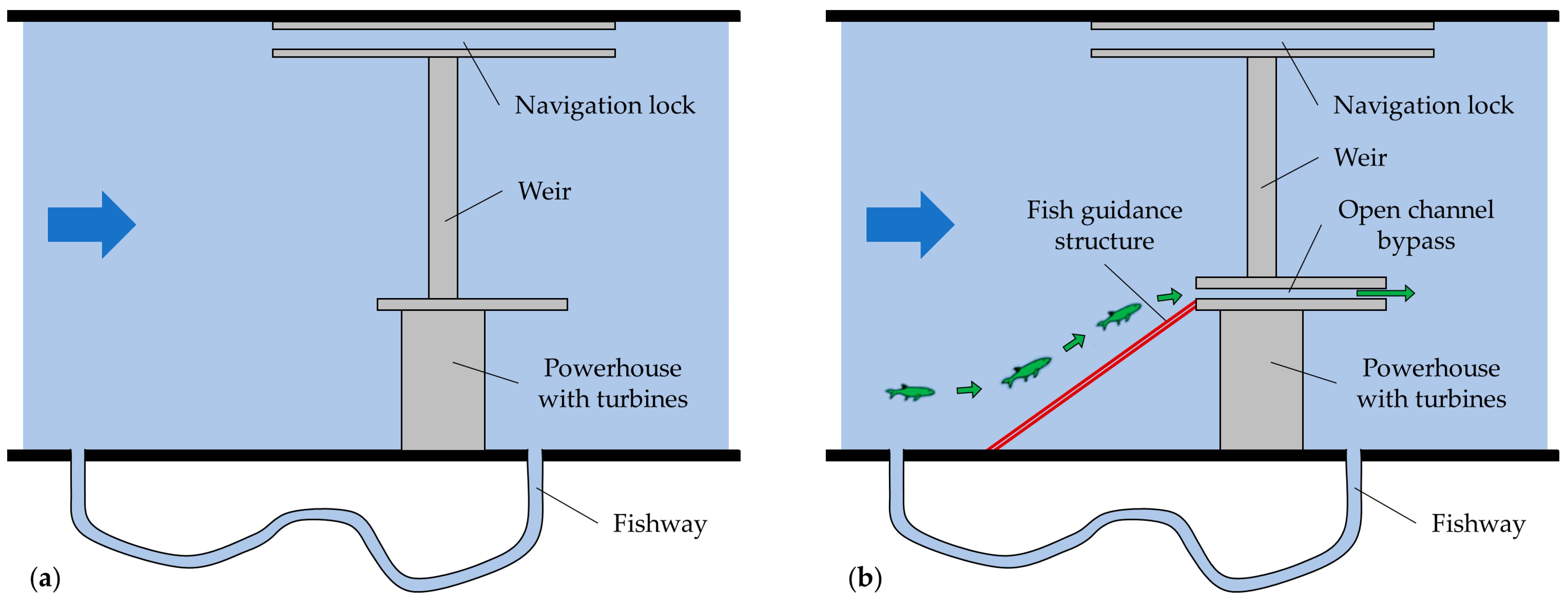
2.1.1. Initial Designs
2.1.2. Variations
2.1.3. Examined Operating Case
2.2. Numerical Models
2.2.1. General
2.2.2. Boundary Conditions
2.2.3. Spatial and Temporal Discretization
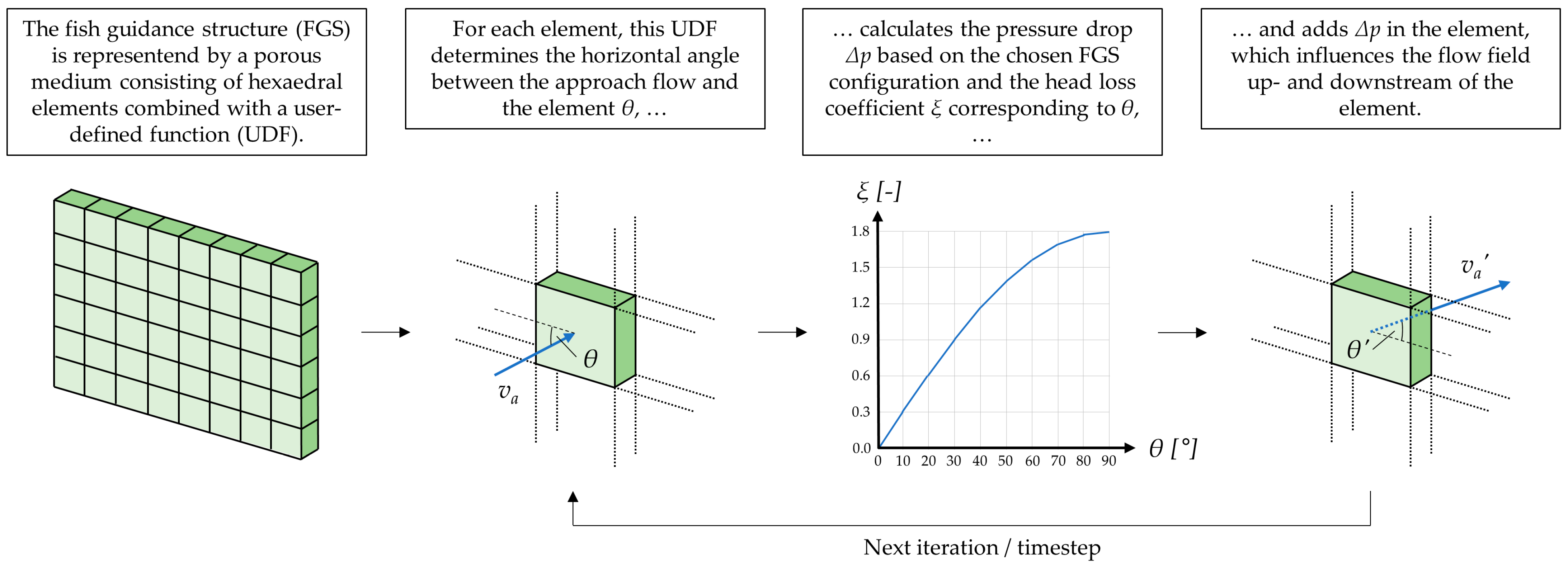
2.2.4. Implementation of the Fish Guidance Structure in the Numerical Model
2.3. Criteria Used for the Evaluation
3. Results
3.1. Overview
3.2. HPP on the Pre-Alpine River
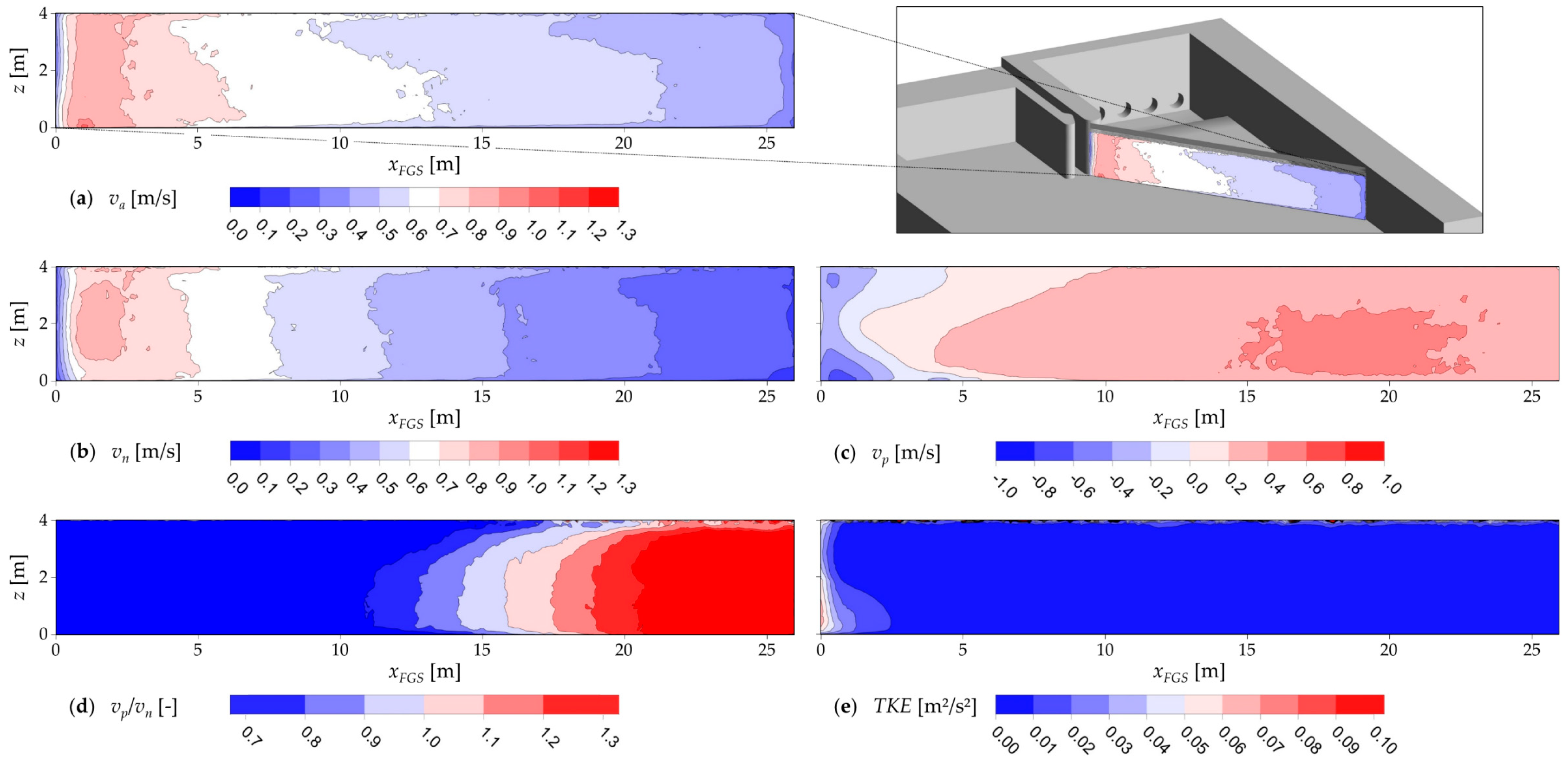
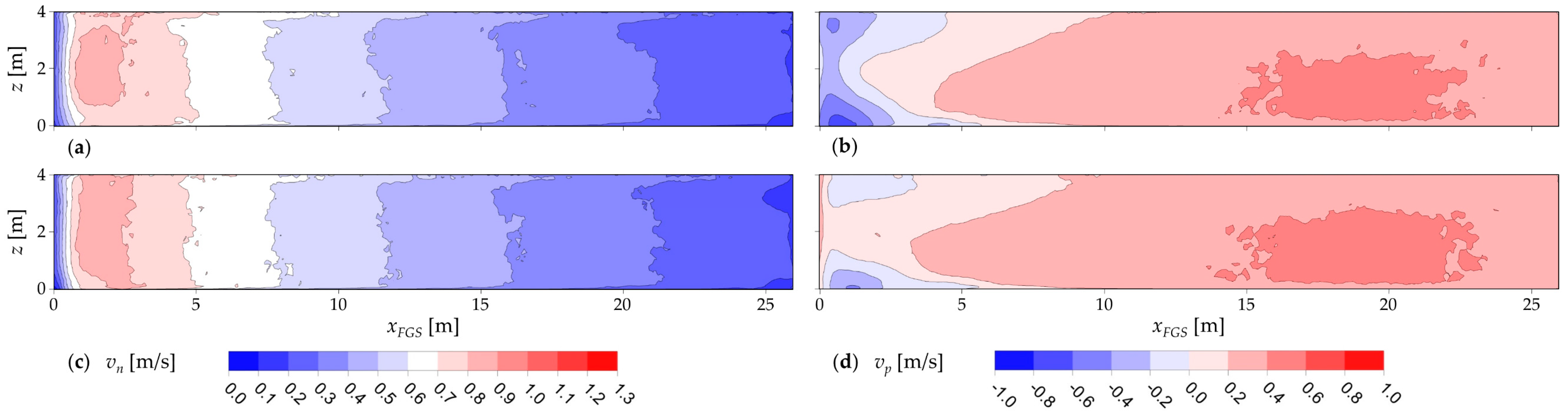
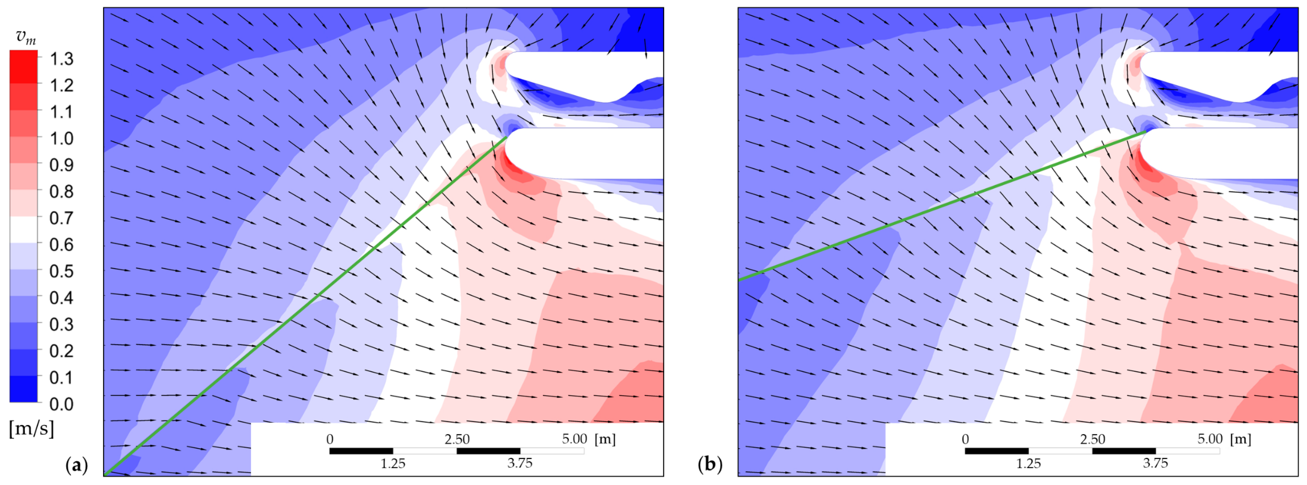
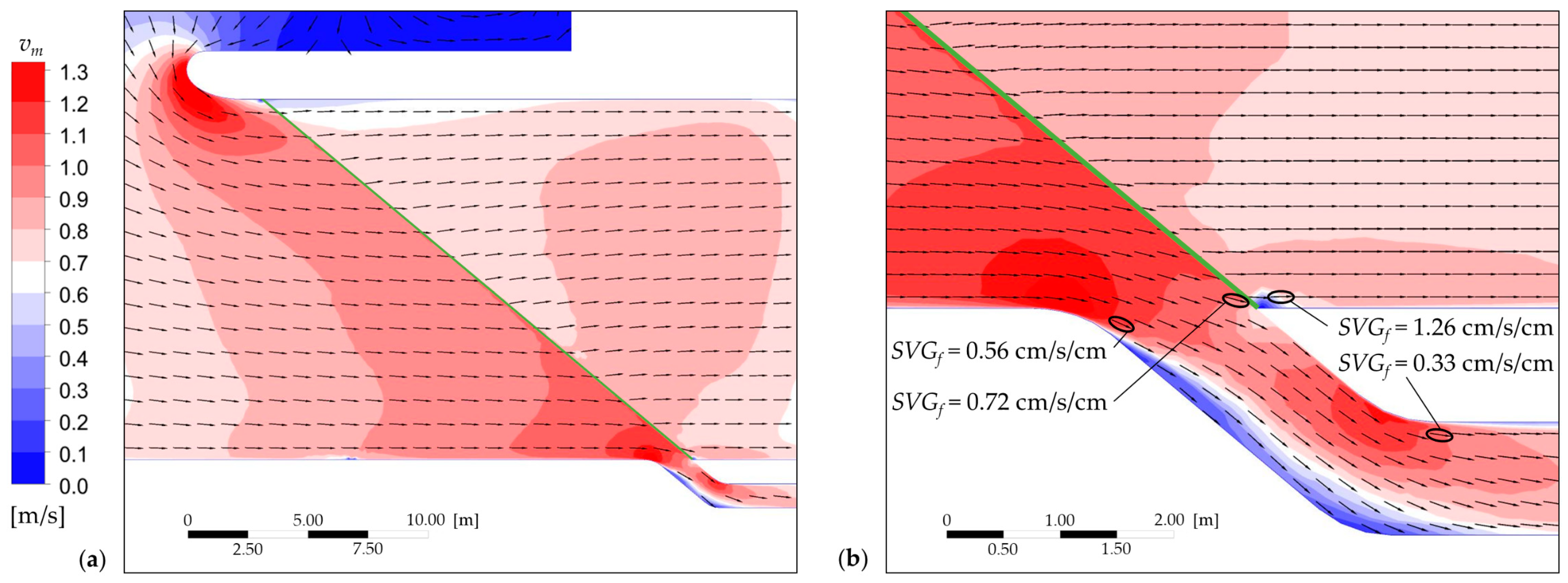
3.2.1. Overall Flow Field
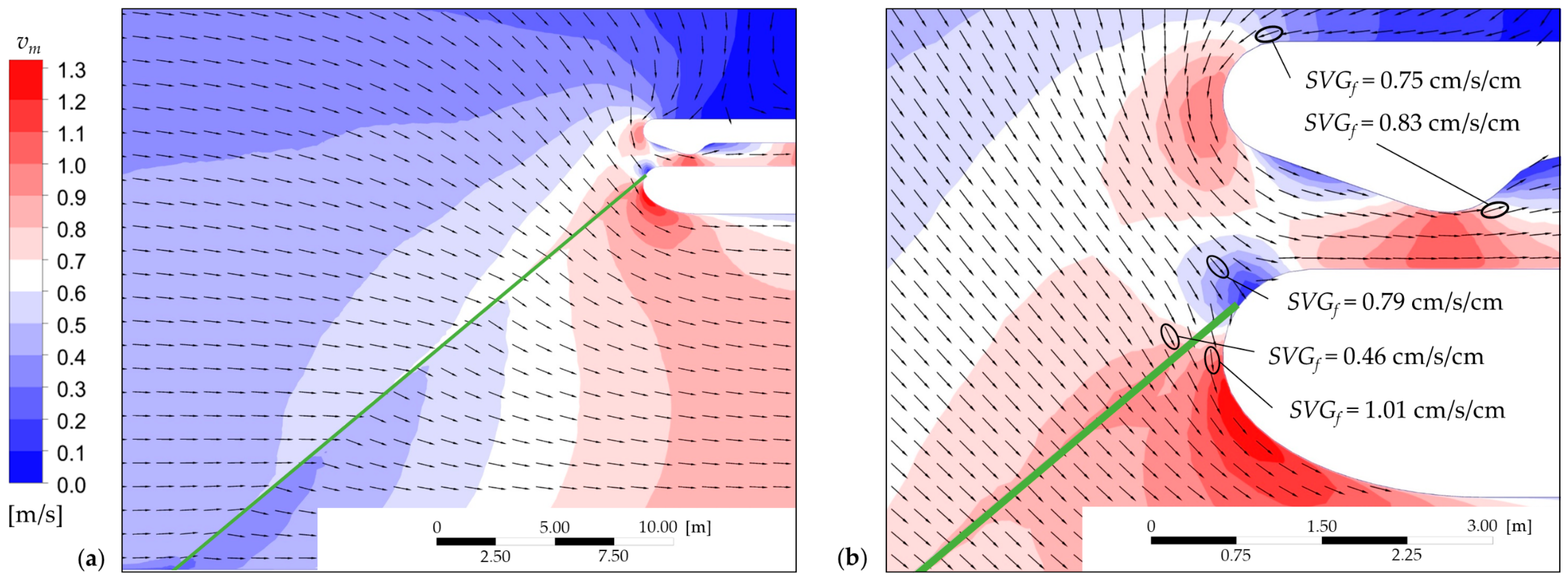
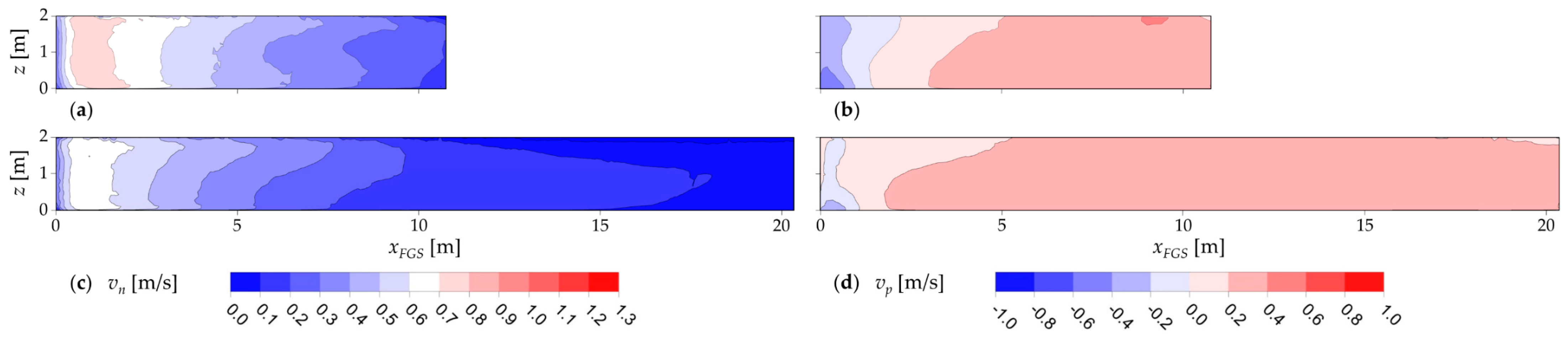
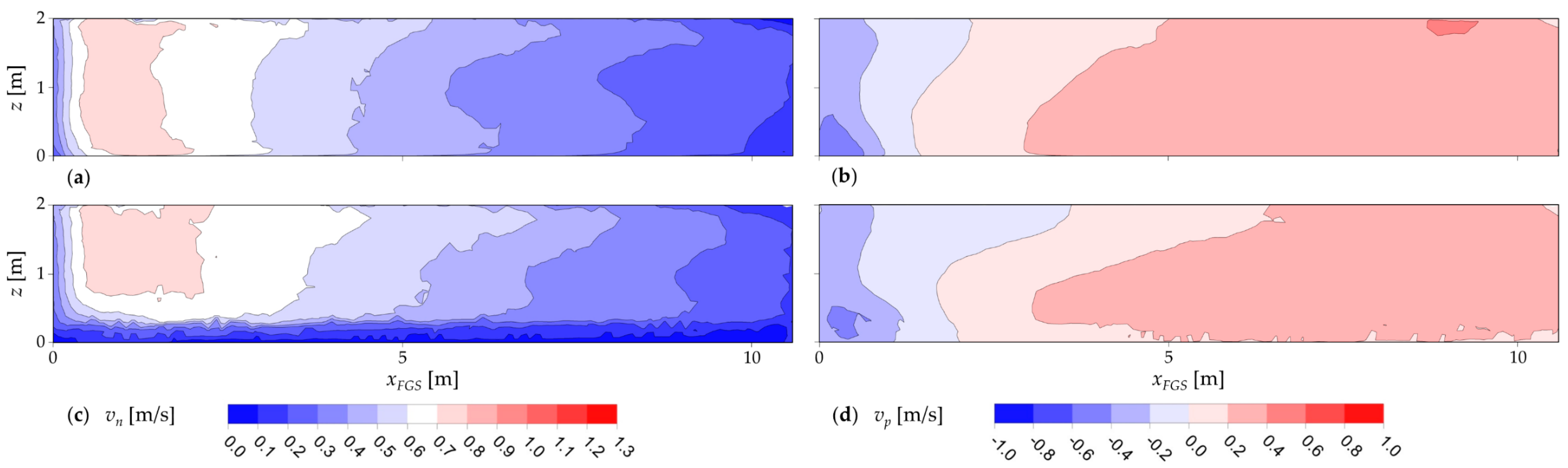
3.2.2. Hydraulic Parameters in Front of the FGS
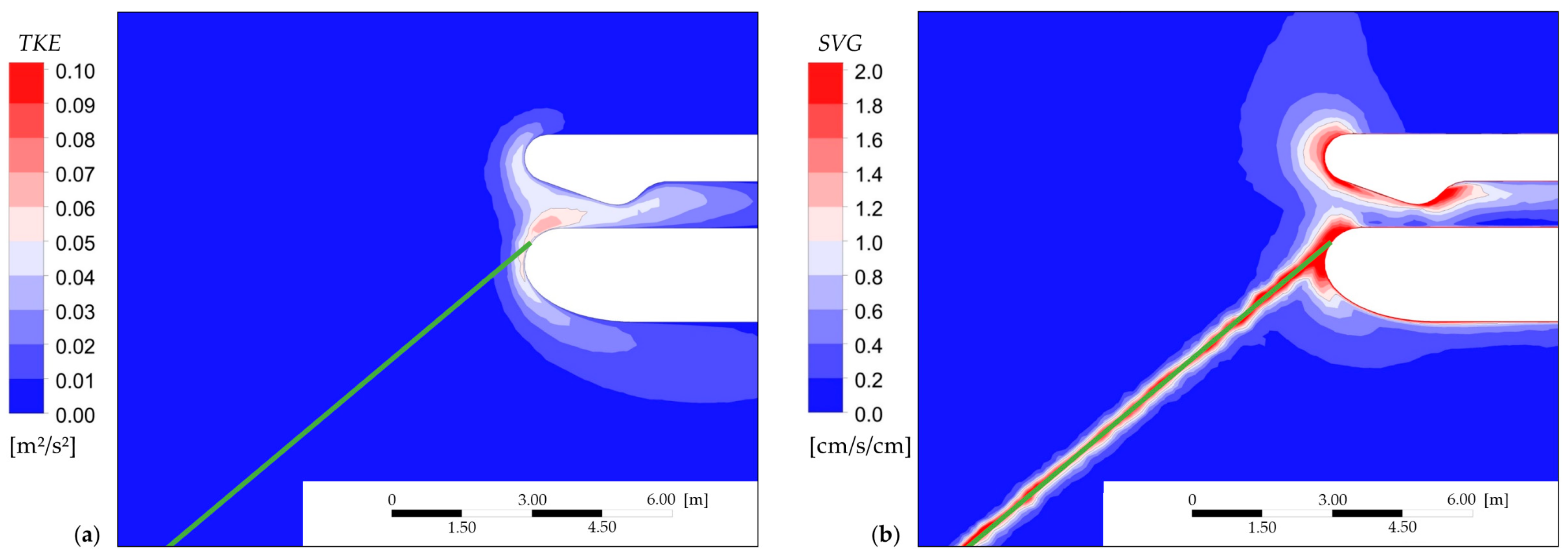
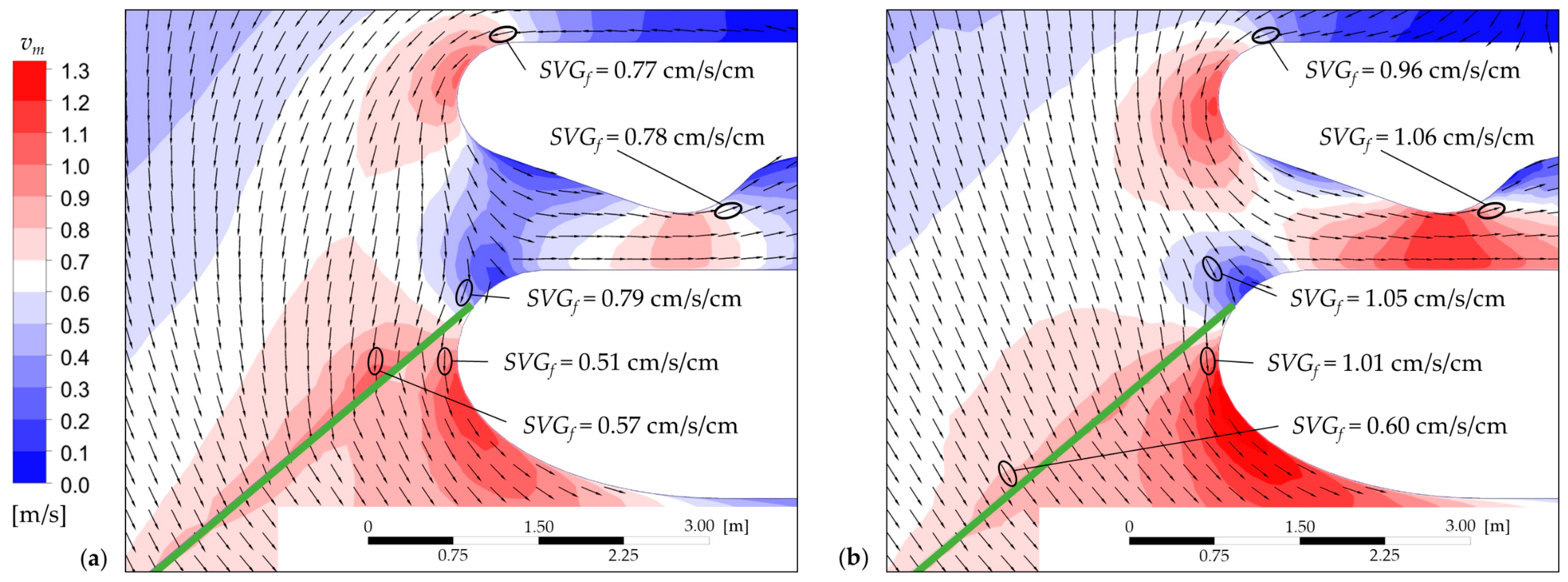
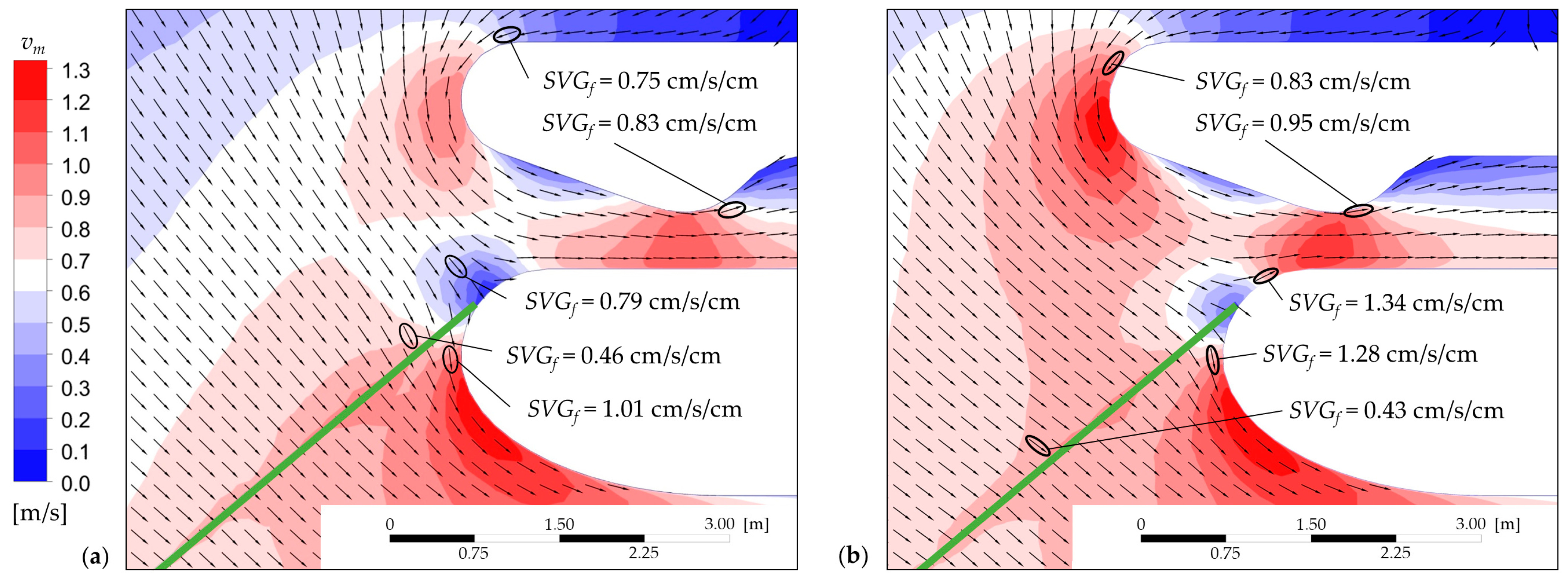
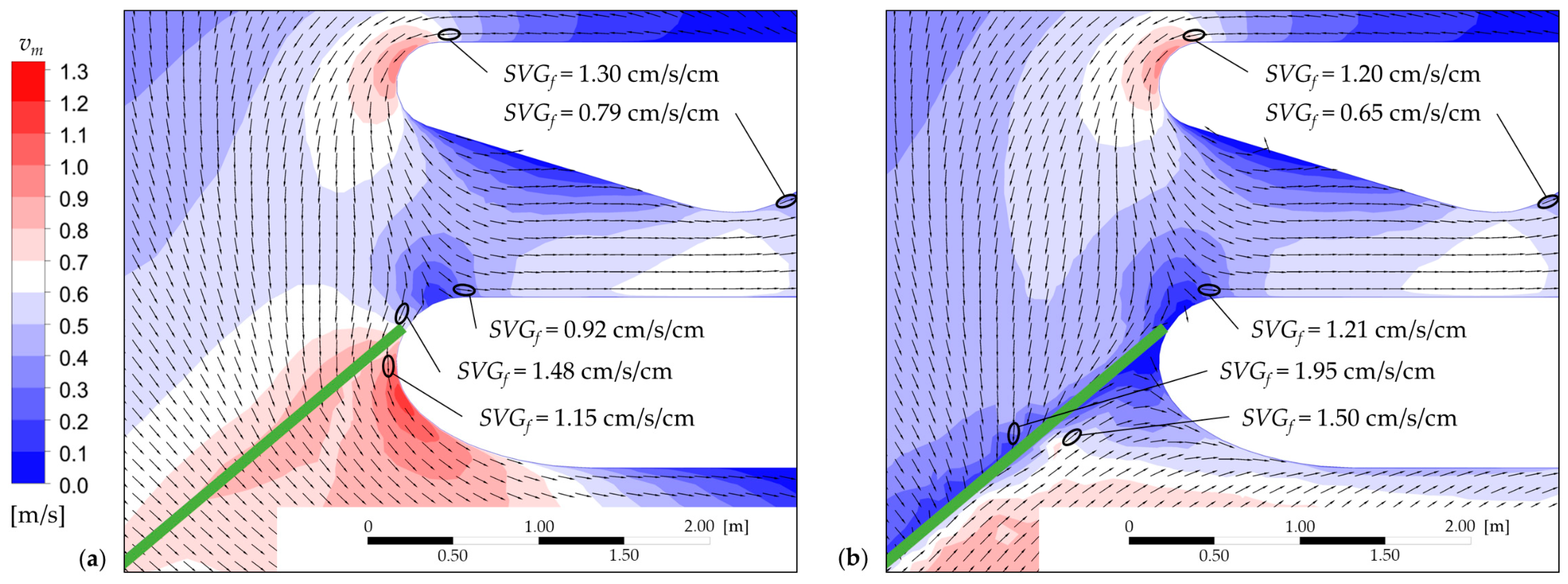
3.2.3. Hydraulic Parameters at the Bypass Entrance
3.3. Variations
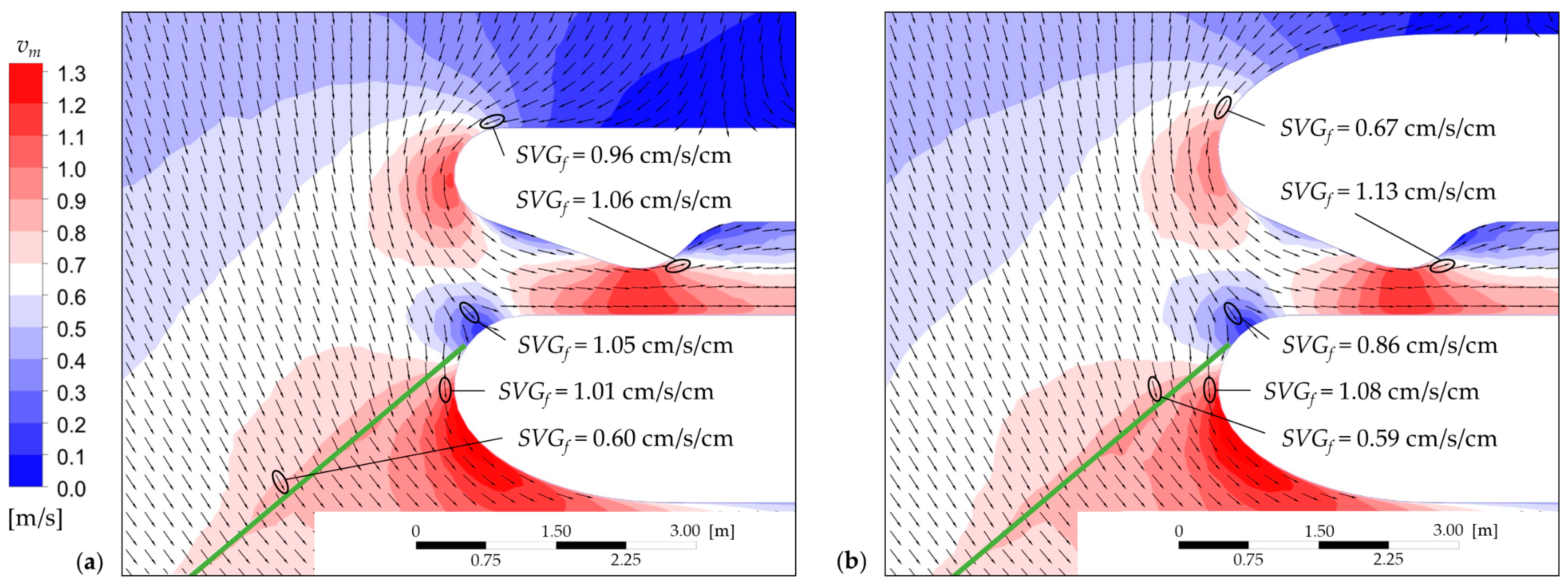
3.3.1. Variation 1 (V1): Shifting the Weir-Side Part of the Dividing Pier 1.0 m in the Upstream Direction
3.3.2. Variation 2 (V2): Changing the Shape and Width of the Weir-Side Part of the Dividing Pier
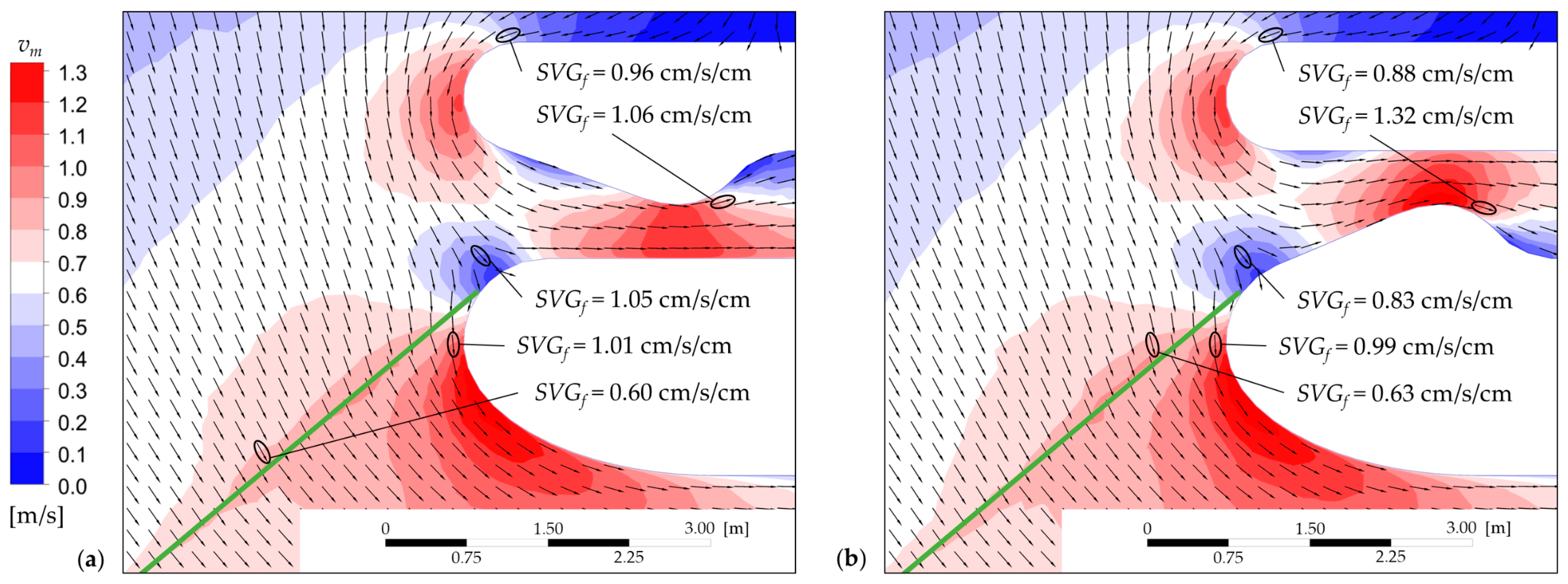
3.3.3. Variation 3 (V3): Installing the Inlet Gate at the Turbine-Side Part of the Dividing Pier
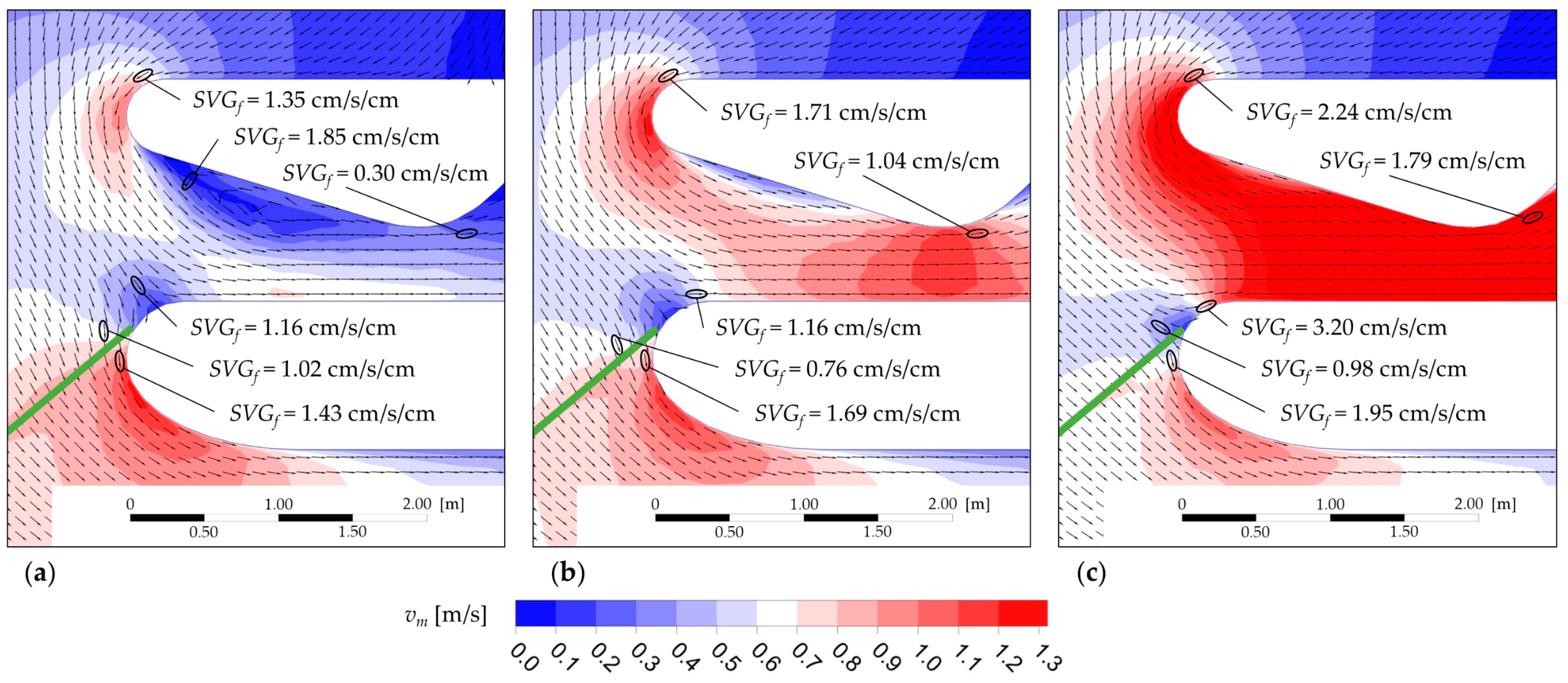
3.3.4. Variation 4 (V4): Doubling Qby by Lowering the Sloping Weir
3.3.5. Variation 5 (V5): Quadrupling Qby by Lowering the Sloping Weir
3.3.6. Variation 6 (V6): Changing α to 20°
3.3.7. Variation 7 (V7): Implementing a Bottom Overlay with a Height of 0.2 m
3.3.8. Variation 8 (V8): Integrating the FGS into the Headrace Channel with the Bypass on the Orographic Right Side
4. Discussion
4.1. Interpretation of the Results and Comparison with the Literature
4.2. Limitations
4.3. Engineering Application Considerations
5. Conclusions
- The block-type layout may lead to large flow deflections towards the turbines, resulting in spatially distinct approach flow conditions to FGSs. Therefore, the use of mean flow values in the design process (e.g., the mean rack normal flow velocity ), as frequently applied in common guidelines, does not allow for an accurate assessment of actual conditions for downstream migrating fish.
- Complex flow conditions with relatively high values for the turbulent kinetic energy TKE and spatial velocity gradient SVG, which often caused avoidance responses in previous ethohydraulic experiments [12,48], can occur especially at the bypass entrance, but may be mostly negligible in the area upstream of the HBRs.
- The flow conditions at the bypass entrance are significantly affected by the bypass discharge Qby, which should be determined based on the hydraulic parameters at the bypass entrance rather than a fixed percentage of the total river discharge Q0, as well as by the geometric design of the entrance area and the bypass itself. In terms of fish guidance efficiency (FGE) along the FGS, the effects are negligible.
- Low rack angles α and the implementation of a bottom overlay can improve the FGE at block-type HPPs from a hydraulic point of view.
Supplementary Materials
Author Contributions
Funding
Institutional Review Board Statement
Data Availability Statement
Acknowledgments
Conflicts of Interest
Abbreviations
| ASME | American Society of Mechanical Engineers |
| CFD | Computational fluid dynamics |
| DES | Detached eddy simulation |
| FGE | Fish guidance efficiency |
| FGS | Fish guidance structure |
| GCI | Grid convergence index |
| HBR | Horizontal bar rack |
| HBR-BS | Horizontal bar rack bypass system |
| HPP | Hydropower plant |
| LES | Large eddy simulation |
| L1–L5 | Locations 1 to 5 |
| MFS | Maximum face sizing |
| RANS | Reynolds-averaged Navier-Stokes |
| SIMPLE | Semi-Implicit Method for Pressure-Linked Equations |
| UDF | User-defined function |
| VBR | Vertical bar rack |
| V1–V8 | Variations 1 to 8 |
| WFD | Water framework directive |
| Notation | |
| AFGS,hyd | Hydraulically active area of the FGS [m2] |
| hbo | Bottom overlay height [m] |
| h0 | Approach water level upstream of the HPP [m] |
| lFGS | Length of the FGS [m] |
| Qby | Bypass discharge [m3/s] |
| Qby,rel | Relative bypass discharge [-] |
| Qd | Design discharge [m3/s] |
| Q0 | (Assumed) total river discharge [m3/s] |
| r | Grid refinement factor [-] |
| SVG | Spatial velocity gradient [1/s or cm/s/cm] |
| SVGf | Spatial velocity gradient experienced by a fish [1/s or cm/s/cm] |
| T | Water temperature [°C] |
| t | Swimming duration [s] |
| TKE | Turbulent kinetic energy [m2/s2] |
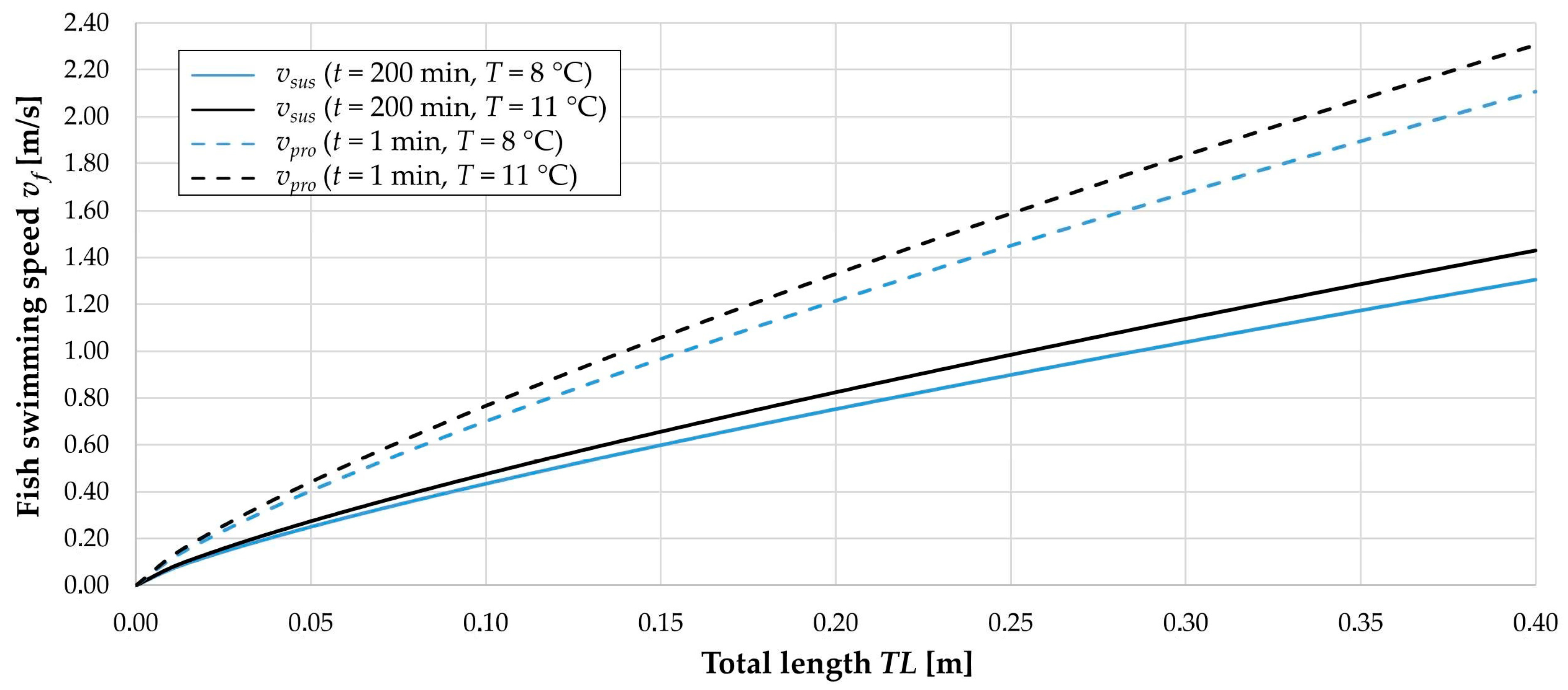
| TL | Total fish length [m] |
| u’, v’, w’ | Local flow velocity fluctuations in x-, y-, and z-direction [m/s] |
| u, v, w | Local flow velocities in x-, y-, and z-direction [m/s] |
| va | Approach flow velocity to the FGS [m/s] |
| va’ | Outflow velocity downstream of the FGS [m/s] |
| vby | Velocity at the bypass entrance [m/s] |
| vf | Fish swimming speed [m/s] |
| vm | Velocity magnitude [m/s] |
| vn | Rack normal velocity component [m/s] |
| vp | Rack parallel velocity component [m/s] |
| vpro | Prolonged swimming speed [m/s] |
| vsus | Sustained swimming speed [m/s] |
| v0 | Mean approach flow velocity [m/s] |
| wby | Bypass width [m] |
| w0 | River width [m] |
| x, y, z | Coordinates [-] |
| α | Horizontal rack angle [°] |
| αw | Water volume fraction parameter [-] |
| Δh | Water level difference [m] |
| Δp | Pressure drop [Pa] |
| θ | Horizontal angle between the approach flow and FGS [°] |
| θ’ | Horizontal angle between the outflow and FGS downstream of the FGS [°] |
| ξ | Head loss coefficient [-] |
Appendix A

| Mesh | MFS Outer/Inner Region [m] | Elements | r [-] | L1 | L2 | GCI [%] L3 | L4 | L5 |
|---|---|---|---|---|---|---|---|---|
| Fine | 0.2/0.1 | 4,039,279 | 2.152 1.864 | 1.902 16.305 | 0.507 3.599 | 1.453 11.614 | 1.714 3.436 | 0.275 1.477 |
| Medium | 0.4/0.2 | 810,298 | ||||||
| Coarse | 0.8/0.4 | 250,128 |
References
- International Hydropower Association (IHA). Hydropower Status Report 2021. Sector Trends and Insights; International Hydropower Association (IHA): London, UK, 2021. [Google Scholar]
- European Commission, Joint Research Centre. Hydropower: Technology Market Report; Publications Office: Luxembourg, Luxembourg, 2019. [Google Scholar]
- Quaranta, E.; Aggidis, G.; Boes, R.M.; Comoglio, C.; De Michele, C.; Ritesh Patro, E.; Georgievskaia, E.; Harby, A.; Kougias, I.; Muntean, S.; et al. Assessing the Energy Potential of Modernizing the European Hydropower Fleet. Energy Convers. Manag. 2021, 246, 114655. [Google Scholar] [CrossRef]
- Directive, Strategic Environmental Assessment. European Commission Directive 2000/60/EC of the European Parliament and of the Council of 23 October 2000 Establishing a Framework for Community Action in the Field of Water Policy. Off. J. Eur. Communities 2000, 22, 2000. [Google Scholar]
- Lucas, M.C.; Baras, E. Migration of Freshwater Fishes; Blackwell Science: Oxford, UK; Malden, MA, USA, 2001; ISBN 978-0-632-05754-2. [Google Scholar]
- Williams, J.G. Mitigating the Effects of High-Head Dams on the Columbia River, USA: Experience from the Trenches. Hydrobiologia 2008, 609, 241–251. [Google Scholar] [CrossRef]
- Best, J. Anthropogenic Stresses on the World’s Big Rivers. Nature Geosci. 2019, 12, 7–21. [Google Scholar] [CrossRef]
- Ekka, A.; Pande, S.; Jiang, Y.; der Zaag, P. van Anthropogenic Modifications and River Ecosystem Services: A Landscape Perspective. Water 2020, 12, 2706. [Google Scholar] [CrossRef]
- Chong, X.Y.; Vericat, D.; Batalla, R.J.; Teo, F.Y.; Lee, K.S.P.; Gibbins, C.N. A Review of the Impacts of Dams on the Hydromorphology of Tropical Rivers. Sci. Total Environ. 2021, 794, 148686. [Google Scholar] [CrossRef]
- Pavlov, D.S. Structures Assisting the Migrations of Non-Salmonid Fish: USSR; FAO fisheries technical paper; Food and Agriculture Organization of the United Nations: Rome, Italy, 1989; ISBN 978-92-5-102857-5. [Google Scholar]
- Larinier, M.; Travade, F. Downstream Migration: Problems and Facilities. Bull. Fr. Pêche Piscic. 2002, 364, 181–207. [Google Scholar] [CrossRef] [Green Version]
- Enders, E.C.; Gessel, M.H.; Williams, J.G. Development of Successful Fish Passage Structures for Downstream Migrants Requires Knowledge of Their Behavioural Response to Accelerating Flow. Can. J. Fish. Aquat. Sci. 2009, 66, 2109–2117. [Google Scholar] [CrossRef]
- Calles, O.; Greenberg, L. Connectivity Is a Two-Way Street-the Need for a Holistic Approach to Fish Passage Problems in Regulated Rivers: Connectivity Is a Two-Way Street. River Res. Applic. 2009, 25, 1268–1286. [Google Scholar] [CrossRef]
- Anderson, D.; Moggridge, H.; Warren, P.; Shucksmith, J. The Impacts of ‘Run-of-River’ Hydropower on the Physical and Ecological Condition of Rivers: Physical and Ecological Impacts of ROR Hydropower. Water Environ. J. 2015, 29, 268–276. [Google Scholar] [CrossRef] [Green Version]
- Huusko, R.; Hyvärinen, P.; Jaukkuri, M.; Mäki-Petäys, A.; Orell, P.; Erkinaro, J. Survival and Migration Speed of Radio-Tagged Atlantic Salmon (Salmo salar) Smolts in Two Large Rivers: One without and One with Dams. Can. J. Fish. Aquat. Sci. 2018, 75, 1177–1184. [Google Scholar] [CrossRef]
- Silva, A.T.; Lucas, M.C.; Castro-Santos, T.; Katopodis, C.; Baumgartner, L.J.; Thiem, J.D.; Aarestrup, K.; Pompeu, P.S.; O’Brien, G.C.; Braun, D.C.; et al. The Future of Fish Passage Science, Engineering, and Practice. Fish Fish. 2018, 19, 340–362. [Google Scholar] [CrossRef] [Green Version]
- Dingle, H.; Drake, V.A. What Is Migration? BioScience 2007, 57, 113–121. [Google Scholar] [CrossRef] [Green Version]
- Zitek, A.; Schmutz, S.; Unfer, G.; Ploner, A. Fish Drift in a Danube Sidearm-System: I. Site-, Inter- and Intraspecific Patterns. J. Fish Biol. 2004, 65, 1319–1338. [Google Scholar] [CrossRef]
- Bunn, S.E.; Arthington, A.H. Basic Principles and Ecological Consequences of Altered Flow Regimes for Aquatic Biodiversity. Environ. Manag. 2002, 30, 492–507. [Google Scholar] [CrossRef] [PubMed] [Green Version]
- Nilsson, C.; Reidy, C.A.; Dynesius, M.; Revenga, C. Fragmentation and Flow Regulation of the World’s Large River Systems. Science 2005, 308, 405–408. [Google Scholar] [CrossRef] [Green Version]
- Goodwin, R.A.; Politano, M.; Garvin, J.W.; Nestler, J.M.; Hay, D.; Anderson, J.J.; Weber, L.J.; Dimperio, E.; Smith, D.L.; Timko, M. Fish Navigation of Large Dams Emerges from Their Modulation of Flow Field Experience. Proc. Natl. Acad. Sci. USA 2014, 111, 5277–5282. [Google Scholar] [CrossRef] [Green Version]
- Ovidio, M.; Dierckx, A.; Bunel, S.; Grandry, L.; Spronck, C.; Benitez, J.P. Poor Performance of a Retrofitted Downstream Bypass Revealed by the Analysis of Approaching Behaviour in Combination with a Trapping System: Retrofitted Downstream Bypass System. River Res. Applic. 2017, 33, 27–36. [Google Scholar] [CrossRef]
- Haraldstad, T.; Höglund, E.; Kroglund, F.; Haugen, T.O.; Forseth, T. Common Mechanisms for Guidance Efficiency of Descending Atlantic Salmon Smolts in Small and Large Hydroelectric Power Plants: Guidance Efficiency of Descending Smolts at Hydroelectric Power Plants. River Res. Applic. 2018, 34, 1179–1185. [Google Scholar] [CrossRef]
- Katopodis, C.; Williams, J.G. The Development of Fish Passage Research in a Historical Context. Ecol. Eng. 2012, 48, 8–18. [Google Scholar] [CrossRef]
- Nyqvist, D.; Elghagen, J.; Heiss, M.; Calles, O. An Angled Rack with a Bypass and a Nature-like Fishway Pass Atlantic Salmon Smolts Downstream at a Hydropower Dam. Mar. Freshw. Res. 2018, 69, 1894. [Google Scholar] [CrossRef]
- Turnpenny, A.W.H.; O’Keeffe, N. Screening for Intake and Outfalls: A Best Practice Guide; Environment Agency: Bristol, UK, 2005; ISBN 978-1-84432-361-6.
- Feigenwinter, L.; Vetsch, D.; Kammerer, S.; Kriewitz, C.; Boes, R. Conceptual Approach for Positioning of Fish Guidance Structures Using CFD and Expert Knowledge. Sustainability 2019, 11, 1646. [Google Scholar] [CrossRef] [Green Version]
- Ebel, G. Fischschutz und Fischabstieg an Wasserkraftanlagen: Handbuch Rechen- und Bypasssysteme: Ingenieurbiologische Grundlagen, Modellierung und Prognose, Bemessung und Gestaltung; Mitteilungen aus dem Büro für Gewässerökologie und Fischereibiologie Dr. Ebel; 3. Auflage.; Büro für Gewässerökologie und Fischereibiologie Dr. Ebel: Halle (Saale), Germany, 2018; ISBN 978-3-00-039686-1. (In German) [Google Scholar]
- Williams, J.G.; Armstrong, G.; Katopodis, C.; Larinier, M.; Travade, F. Thinking like a Fish: A Key Ingredient for Developement of Effective Fish Passage Facilities at River Obstructions: Fish Behaviour Related Fish Passage at Dams. River Res. Applic. 2012, 28, 407–417. [Google Scholar] [CrossRef] [Green Version]
- Kammerlander, H.; Schlosser, L.; Zeiringer, B.; Unfer, G.; Zeileis, A.; Aufleger, M. Downstream Passage Behavior of Potamodromous Fishes at the Fish Protection and Guidance System “Flexible Fish Fence”. Ecol. Eng. 2020, 143, 105698. [Google Scholar] [CrossRef]
- Russon, I.J.; Kemp, P.S.; Calles, O. Response of Downstream Migrating Adult European Eels (Anguilla anguilla) to Bar Racks under Experimental Conditions: Eel Response to Screens. Ecol. Freshw. Fish 2010, 19, 197–205. [Google Scholar] [CrossRef]
- Gosset, C.; Travade, F.; Durif, C.; Rives, J.; Elie, P. Tests of Two Types of Bypass for Downstream Migration of Eels at a Small Hydroelectric Power Plant. River Res. Applic. 2005, 21, 1095–1105. [Google Scholar] [CrossRef]
- Wagner, F. Fact Sheet 05—Wann Ist Ein Rechen Ein Fischschutzrechen? Die Funktionalen Elemente Eines Fischschutzsystems; Forum Fischschutz & Fischabstieg: Berlin, Germany, 2021. (In German) [Google Scholar]
- BAFU. Wiederherstellung Der Fischwanderung. Gute Praxisbeispiele Für Wasserkraftanlagen in Der Schweiz; Umwelt-Wissen Nr. 2205; Bundesamt für Umwelt: Berlin, Germany, 2022. (In German) [Google Scholar]
- de Bie, J.; Peirson, G.; Kemp, P.S. Effectiveness of Horizontally and Vertically Oriented Wedge-Wire Screens to Guide Downstream Moving Juvenile Chub (Squalius cephalus). Ecol. Eng. 2018, 123, 127–134. [Google Scholar] [CrossRef]
- Harbicht, A.B.; Watz, J.; Nyqvist, D.; Virmaja, T.; Carlsson, N.; Aldvén, D.; Nilsson, P.A.; Calles, O. Guiding Migrating Salmonid Smolts: Experimentally Assessing the Performance of Angled and Inclined Screens with Varying Gap Widths. Ecol. Eng. 2022, 174, 106438. [Google Scholar] [CrossRef]
- Meister, J. Fish Protection and Guidance at Water Intakes with Horizontal Bar Rack Bypass Systems. VAW-Mitteilungen 2020, 258. [Google Scholar] [CrossRef]
- Meister, J.; Fuchs, H.; Beck, C.; Albayrak, I.; Boes, R.M. Head Losses of Horizontal Bar Racks as Fish Guidance Structures. Water 2020, 12, 475. [Google Scholar] [CrossRef] [Green Version]
- Maddahi, M.; Hagenbüchli, R.; Mendez, R.; Zaugg, C.; Boes, R.M.; Albayrak, I. Field Investigation of Hydraulics and Fish Guidance Efficiency of a Horizontal Bar Rack-Bypass System. Water 2022, 14, 776. [Google Scholar] [CrossRef]
- Meister, J.; Selz, O.M.; Beck, C.; Peter, A.; Albayrak, I.; Boes, R.M. Protection and Guidance of Downstream Moving Fish with Horizontal Bar Rack Bypass Systems. Ecol. Eng. 2022, 178, 106584. [Google Scholar] [CrossRef] [PubMed]
- Meister, J.; Fuchs, H.; Beck, C.; Albayrak, I.; Boes, R.M. Velocity Fields at Horizontal Bar Racks as Fish Guidance Structures. Water 2020, 12, 280. [Google Scholar] [CrossRef] [Green Version]
- U.S. Department of the Interior. Fish Protection at Water Diversions: A Guide for Planning and Designing Fish Exclusion Facilities; Water Resources Technical Publication, Bureau of Reclamation: Denver, CO, USA, 2006.
- Boes, R.M.; Beck, C.; Meister, J.; Peter, A.; Kastinger, M.; Albayrak, I. Effect of Bypass Layout on Guidance of Downstream Moving Fish at Bar Rack Bypass Systems. In Proceedings of the 39th IAHR World Congress, Granada, Spain, 19–24 June 2022; pp. 1312–1321. [Google Scholar]
- Tutzer, R.; Röck, S.; Walde, J.; Zeiringer, B.; Unfer, G.; Führer, S.; Brinkmeier, B.; Haug, J.; Aufleger, M. Ethohydraulic Experiments on the Fish Protection Potential of the Hybrid System FishProtector at Hydropower Plants. Ecol. Eng. 2021, 171, 106370. [Google Scholar] [CrossRef]
- Haro, A.; Odeh, M.; Noreika, J.; Castro-Santos, T. Effect of Water Acceleration on Downstream Migratory Behavior and Passage of Atlantic Salmon Smolts and Juvenile American Shad at Surface Bypasses. Trans. Am. Fish. Soc. 1998, 127, 118–127. [Google Scholar] [CrossRef]
- de Bie, J.; Peirson, G.; Kemp, P.S. Evaluation of Horizontally and Vertically Aligned Bar Racks for Guiding Downstream Moving Juvenile Chub (Squalius cephalus) and Barbel (Barbus barbus). Ecol. Eng. 2021, 170, 106327. [Google Scholar] [CrossRef]
- Silva, A.T.; Bærum, K.M.; Hedger, R.D.; Baktoft, H.; Fjeldstad, H.-P.; Gjelland, K.Ø.; Økland, F.; Forseth, T. The Effects of Hydrodynamics on the Three-Dimensional Downstream Migratory Movement of Atlantic Salmon. Sci. Total Environ. 2020, 705, 135773. [Google Scholar] [CrossRef]
- Liao, J.C. A Review of Fish Swimming Mechanics and Behaviour in Altered Flows. Phil. Trans. R. Soc. B 2007, 362, 1973–1993. [Google Scholar] [CrossRef] [Green Version]
- Silva, A.T.; Santos, J.M.; Ferreira, M.T.; Pinheiro, A.N.; Katopodis, C. Effects of Water Velocity and Turbulence on the Behaviour of Iberian Barbel (Luciobarbus bocagei, Steindachner 1864) in an Experimental Pool-Type Fishway: IBERIAN BARBEL’S RESPONSE TO VELOCITY AND TURBULENCE. River Res. Applic. 2011, 27, 360–373. [Google Scholar] [CrossRef]
- Vowles, A.S.; Kemp, P.S. Effects of Light on the Behaviour of Brown Trout (Salmo trutta) Encountering Accelerating Flow: Application to Downstream Fish Passage. Ecol. Eng. 2012, 47, 247–253. [Google Scholar] [CrossRef]
- Szabo-Meszaros, M.; Forseth, T.; Baktoft, H.; Fjeldstad, H.; Silva, A.T.; Gjelland, K.Ø.; Økland, F.; Uglem, I.; Alfredsen, K. Modelling Mitigation Measures for Smolt Migration at Dammed River Sections. Ecohydrology 2019, 12, e2131. [Google Scholar] [CrossRef]
- Foldvik, A.; Silva, A.T.; Albayrak, I.; Schwarzwälder, K.; Boes, R.M.; Ruther, N. Combining Fish Passage and Sediment Bypassing: A Conceptual Solution for Increased Sustainability of Dams and Reservoirs. Water 2022, 14, 1977. [Google Scholar] [CrossRef]
- Li, P.; Zhang, W.; Burnett, N.J.; Zhu, D.Z.; Casselman, M.; Hinch, S.G. Evaluating Dam Water Release Strategies for Migrating Adult Salmon Using Computational Fluid Dynamic Modeling and Biotelemetry. Water Resour. Res. 2021, 57, e2020WR028981. [Google Scholar] [CrossRef]
- Gisen, D.C.; Weichert, R.B.; Nestler, J.M. Optimizing Attraction Flow for Upstream Fish Passage at a Hydropower Dam Employing 3D Detached-Eddy Simulation. Ecol. Eng. 2017, 100, 344–353. [Google Scholar] [CrossRef] [Green Version]
- Quaranta, E.; Katopodis, C.; Revelli, R.; Comoglio, C. Turbulent Flow Field Comparison and Related Suitability for Fish Passage of a Standard and a Simplified Low-Gradient Vertical Slot Fishway. River Res. Applic. 2017, 33, 1295–1305. [Google Scholar] [CrossRef]
- Fuentes-Pérez, J.F.; Silva, A.T.; Tuhtan, J.A.; García-Vega, A.; Carbonell-Baeza, R.; Musall, M.; Kruusmaa, M. 3D Modelling of Non-Uniform and Turbulent Flow in Vertical Slot Fishways. Environ. Model. Softw. 2018, 99, 156–169. [Google Scholar] [CrossRef]
- Heneka, P.; Zinkhahn, M.; Schütz, C.; Weichert, R.B. A Parametric Approach for Determining Fishway Attraction Flow at Hydropower Dams. Water 2021, 13, 743. [Google Scholar] [CrossRef]
- Szabo-Meszaros, M.; Silva, A.; Bærum, K.; Baktoft, H.; Alfredsen, K.; Hedger, R.; Økland, F.; Gjelland, K.; Fjeldstad, H.-P.; Calles, O.; et al. Validation of a Swimming Direction Model for the Downstream Migration of Atlantic Salmon Smolts. Water 2021, 13, 1230. [Google Scholar] [CrossRef]
- Ben Jebria, N.; Carmigniani, R.; Drouineau, H.; De Oliveira, E.; Tétard, S.; Capra, H. Coupling 3D Hydraulic Simulation and Fish Telemetry Data to Characterize the Behaviour of Migrating Smolts Approaching a Bypass. J. Ecohydraulics 2021, 1–14. [Google Scholar] [CrossRef]
- Lundström, T.S.; Hellström, J.G.I.; Lindmark, E.M. Flow Design of Guiding Device for Downstream Fish Migration. River Res. Applic. 2009, 26, 166–182. [Google Scholar] [CrossRef]
- Lundström, T.S.; Brynell-Rahkola, M.; Ljung, A.-L.; Hellström, J.G.I.; Green, T.M. Evaluation of Guiding Device for Downstream Fish Migration with In-Field Particle Tracking Velocimetry and CFD. J. Appl. Fluid Mech. 2015, 8, 579–589. [Google Scholar] [CrossRef]
- Mulligan, K.B.; Towler, B.; Haro, A.; Ahlfeld, D.P. A Computational Fluid Dynamics Modeling Study of Guide Walls for Downstream Fish Passage. Ecol. Eng. 2017, 99, 324–332. [Google Scholar] [CrossRef] [Green Version]
- Mulligan, K.B.; Towler, B.; Haro, A.; Ahlfeld, D.P. Sensitivity of the Downward to Sweeping Velocity Ratio to the Bypass Flow Percentage along a Guide Wall for Downstream Fish Passage. Ecol. Eng. 2017, 109, 10–14. [Google Scholar] [CrossRef]
- Zöschg, H.; Haug, J.; Tutzer, R.; Zeiringer, B.; Unfer, G.; Stoltz, U.; Aufleger, M. Fischschutz und Anströmung an Wasserkraftanlagen mit niedrigen Fallhöhen. Wasserwirtsch 2021, 111, 36–42. (In German) [Google Scholar] [CrossRef]
- Giesecke, J.; Heimerl, S. Wasserkraftanlagen: Planung, Bau und Betrieb; Springer: Berlin/Heidelberg, Germany, 2014; ISBN 978-3-642-53871-1. (In German) [Google Scholar]
- Haunschmid, R.; Wolfram, G.; Spindler, T.; Honsig-Erlenburg, W.; Wimmer, R.; Jagsch, A.; Kainz, E.; Hehenwarter, K.; Wagner, B.; Konecny, R.; et al. Erstellung Einer Fischbasierten Typologie Österreichischer Fließgewässer Sowie Einer Bewertungsmethode Des Fischökologischen Zustandes Gemäß EU-Wasserrahmenrichtlinie; Schriftenreihe des BAW, Band 23; Bundesamt für Wasserwirtschaft: Wien, Germany, 2006. (In German) [Google Scholar]
- Häusler, E. Wehre. Wasserbauten aus Beton; Handbuch für Beton-, Stahlbeton- und Spannbetonbau; W. Ernst: Berlin, Germany, 1987; ISBN 978-3-433-01009-9. (In German) [Google Scholar]
- Wagner, F. Vergleichende Analyse des Fischabstiegs an drei Wasserkraftanlagen einer Kraftwerkskette. Wasserwirtsch 2016, 106, 35–41. (In German) [Google Scholar] [CrossRef]
- Hirt, C.W.; Nichols, B.D. Volume of Fluid (VOF) Method for the Dynamics of Free Boundaries. J. Comput. Phys. 1981, 39, 201–225. [Google Scholar] [CrossRef]
- ANSYS, Inc. ANSYS Fluent Theory Guide; Release 19.0.; Southpointe: Canonsburg, PA, USA, 2018. [Google Scholar]
- Celik, I.B.; Ghia, U.; Roache, P.J. Procedure for Estimation and Reporting of Uncertainty Due to Discretization in CFD Applications. J. Fluids Eng. 2008, 130, 078001. [Google Scholar] [CrossRef] [Green Version]
- Meusburger, H. Energieverluste an Einlaufrechen von Flusskraftwerken (Hydraulic Losses at Bar Racks of Run-of-River Plants). Ph.D. Thesis, Laboratory of Hydraulics, Hydrology and Glaciology (VAW), ETH Zurich, Zurich, Switzerland, 2002. (In German). [Google Scholar]
- Böttcher, H.; Gabl, R.; Aufleger, M. Experimental Hydraulic Investigation of Angled Fish Protection Systems—Comparison of Circular Bars and Cables. Water 2019, 11, 1056. [Google Scholar] [CrossRef] [Green Version]
- Cano-Barbacil, C.; Radinger, J.; Argudo, M.; Rubio-Gracia, F.; Vila-Gispert, A.; García-Berthou, E. Key Factors Explaining Critical Swimming Speed in Freshwater Fish: A Review and Statistical Analysis for Iberian Species. Sci. Rep. 2020, 10, 18947. [Google Scholar] [CrossRef]
- Moog, O. Fauna Aquatica Austriaca, Edition 2002; Wasserwirtschaftskataster, Bundesministerium für Land- und Forstwirtschaft, Umwelt und Wasserwirtschaft: Vienna, Austria, 2002. (In German)
- Enders, E.C.; Gessel, M.H.; Anderson, J.J.; Williams, J.G. Effects of Decelerating and Accelerating Flows on Juvenile Salmonid Behavior. Trans. Am. Fish. Soc. 2012, 141, 357–364. [Google Scholar] [CrossRef]
- Albayrak, I.; Boes, R.M.; Kriewitz-Byun, C.R.; Peter, A.; Tullis, B.P. Fish Guidance Structures: Hydraulic Performance and Fish Guidance Efficiencies. J. Ecohydraulics 2020, 5, 113–131. [Google Scholar] [CrossRef]
- Enders, E.C.; Boisclair, D.; Roy, A.G. The Effect of Turbulence on the Cost of Swimming for Juvenile Atlantic Salmon (Salmo salar). Can. J. Fish. Aquat. Sci. 2003, 60, 1149–1160. [Google Scholar] [CrossRef]
- Tritico, H.M.; Cotel, A.J. The Effects of Turbulent Eddies on the Stability and Critical Swimming Speed of Creek Chub (Semotilus atromaculatus). J. Exp. Biol. 2010, 213, 2284–2293. [Google Scholar] [CrossRef] [Green Version]
- Berger, C. Verluste und Auslegung von Schrägrechen anhand ethohydraulischer Studien. Wasserwirtsch 2020, 110, 10–17. (In German) [Google Scholar] [CrossRef]
- Szabo-Meszaros, M.; Navaratnam, C.U.; Aberle, J.; Silva, A.T.; Forseth, T.; Calles, O.; Fjeldstad, H.-P.; Alfredsen, K. Experimental Hydraulics on Fish-Friendly Trash-Racks: An Ecological Approach. Ecol. Eng. 2018, 113, 11–20. [Google Scholar] [CrossRef]
- Knapp, M.; Montgomery, J.; Whittaker, C.; Franklin, P.; Baker, C.; Friedrich, H. Fish Passage Hydrodynamics: Insights into Overcoming Migration Challenges for Small-Bodied Fish. J. Ecohydraulics 2019, 4, 43–55. [Google Scholar] [CrossRef]
- Knott, J.; Mueller, M.; Pander, J.; Geist, J. Bigger than Expected: Species- and Size-Specific Passage of Fish through Hydropower Screens. Ecol. Eng. 2023, 188, 106883. [Google Scholar] [CrossRef]
- Geist, J. Editorial: Green or Red: Challenges for Fish and Freshwater Biodiversity Conservation Related to Hydropower. Aquat. Conserv. Mar. Freshw. Ecosyst. 2021, 31, 1551–1558. [Google Scholar] [CrossRef]
- Silva, A.T.; Bermúdez, M.; Santos, J.M.; Rabuñal, J.R.; Puertas, J. Pool-Type Fishway Design for a Potamodromous Cyprinid in the Iberian Peninsula: The Iberian Barbel—Synthesis and Future Directions. Sustainability 2020, 12, 3387. [Google Scholar] [CrossRef] [Green Version]
- Li, M.; Shi, X.; Jin, Z.; Ke, S.; Lin, C.; An, R.; Li, J.; Katopodis, C. Behaviour and Ability of a Cyprinid (Schizopygopsis younghusbandi) to Cope with Accelerating Flows When Migrating Downstream. River Res. Applic. 2021, 37, 1168–1179. [Google Scholar] [CrossRef]
- Link, O.; Sanhueza, C.; Arriagada, P.; Brevis, W.; Laborde, A.; González, A.; Wilkes, M.; Habit, E. The Fish Strouhal Number as a Criterion for Hydraulic Fishway Design. Ecol. Eng. 2017, 103, 118–126. [Google Scholar] [CrossRef]
- Arenas, A.; Politano, M.; Weber, L.; Timko, M. Analysis of Movements and Behavior of Smolts Swimming in Hydropower Reservoirs. Ecol. Model. 2015, 312, 292–307. [Google Scholar] [CrossRef]
- Whitney, R.R.; Calvin, L.D.; Erho, M.W.; Coutant, C.C. Downstream Passage for Salmon at Hydroelectric Projects in the Columbia River Basin: Development, Installation, and Evaluation; Northwest Power Planning Council: Portland, OR, USA, 1997. [Google Scholar]
- Silva, A.T.; Katopodis, C.; Tachie, M.F.; Santos, J.M.; Ferreira, M.T. Downstream Swimming Behaviour of Catadromous and Potamodromous Fish Over Spillways: Downstream Fish Passage Behaviour Over Spillways. River Res. Applic. 2016, 32, 935–945. [Google Scholar] [CrossRef]
- Nordlund, B. Designing Fish Screens for Fish Protection at Water Diversions; National Marine Fisheries Service: Lacey, WA, USA, 2008.
- Zöschg, H.; Zeiringer, B.; Unfer, G.; Tutzer, R.; Aufleger, M. Numerical Approach for the Evaluation of Downstream Fish Guiding at Low-Head Hydropower Plants. In Proceedings of the 39th IAHR World Congress, Granada, Spain, 19–24 June 2022; pp. 2428–2437. [Google Scholar]
- EPRI; DML. Evaluation of Angled Bar Racks and Louvers for Guiding Fish at Water Intakes; Electric Power Research Institutre (EPRI) and Dominion Millstone Laboratories (DML): Palo Alto, CA, USA; Waterford, NY, USA, 2001. [Google Scholar]
- Schwevers, U.; Adam, B. Fish Protection Technologies and Fish Ways for Downstream Migration; Springer International Publishing: Cham, Switzerland, 2020; ISBN 978-3-030-19241-9. [Google Scholar]
- Gerstner, C.L. Use of Substratum Ripples for Flow Refuging by Atlantic Cod, Gadus Morhua. Environ. Biol. Fishes 1998, 51, 455–460. [Google Scholar] [CrossRef]
- Tutzer, R.; Röck, S.; Walde, J.; Haug, J.; Brinkmeier, B.; Aufleger, M.; Unfer, G.; Führer, S.; Zeiringer, B. A Physical and Behavioral Barrier for Enhancing Fish Downstream Migration at Hydropower Dams: The Flexible FishProtector. Water 2022, 14, 378. [Google Scholar] [CrossRef]
- Haug, J. Examination of the Fish Protection and Guiding Effect of the “Electrified Flexible Fish Fence” Depending on the Electrical Field—Comparison of the Efficiency of the Electrified Flexible Fish Fence with 60 Mm Cable Clearance and 20° Angle of Incidence according to Ethohydraulic Experiments in Lunz Am See. Master’s Thesis, University of Innsbruck, Innsbruck, Austria, 2018. [Google Scholar]
- Pope, S.B. Turbulent Flows; Cambridge University Press: Cambridge, UK; New York, NY, USA, 2000; ISBN 978-0-521-59125-6. [Google Scholar]


| Site | Pre-Alpine River | Alpine River |
|---|---|---|
| Fish Zonation | Grayling Region | Lower Trout Region |
| HPP Construction Type | Block-Type | Block-Type |
| Total river discharge Q0 [m3/s] | 50 | 10 |
| Design discharge Qd [m3/s] | 48 | 8 *, 9 *, 9.5 |
| Bypass discharge Qby [m3/s] | 2 | 0.5, 1 *, 2 * |
| Mean approach flow velocity v0 [m/s] | 0.36 | 0.25 |
| Mean rack normal velocity component [m/s] | 0.46 | 0.24 *, 0.45 |
| River width w0 [m] | 35 | 20 |
| Bypass width wby [m] | 1 | 0.5 |
| Length of the FGS lFGS [m] | 23.34 *, 25.94 | 10.58, 20.19 * |
| Approach water level upstream of the HPP h0 [m] | 4 | 2 |
| Rack angle α [°] | 40 | 20 *, 40 |
| Variation | Varied Component | Description | Schematic Illustration | HPP |
|---|---|---|---|---|
| V1 | Dividing pier (weir-side part) | Shifted 1.0 m in the upstream direction |  | Pre-alpine river |
| V2 | Dividing pier (weir-side part) | Modified the shape and width for smoother flow conditions around the pier |  | Pre-alpine river |
| V3 | Inlet gate | Installed at the turbine-side part of the dividing pier |  | Pre-alpine river |
| V4 | Sloping weir | Lowered to double the bypass discharge Qby compared to the initial design |  | Alpine river |
| V5 | Sloping weir | Lowered to quadruple the bypass discharge Qby compared to the initial design |  | Alpine river |
| V6 | Fish guidance structure | Modified the rack angle α to 20° |  | Alpine river |
| V7 | Fish guidance structure | Implementation of a bottom overlay with a height of 0.2 m |  | Alpine river |
| V8 | Fish guidance structure | Integrated into the headrace channel with the bypass on the orographic right side (cf. Figure 2) |  | Pre-alpine river |
Disclaimer/Publisher’s Note: The statements, opinions and data contained in all publications are solely those of the individual author(s) and contributor(s) and not of MDPI and/or the editor(s). MDPI and/or the editor(s) disclaim responsibility for any injury to people or property resulting from any ideas, methods, instructions or products referred to in the content. |
© 2023 by the authors. Licensee MDPI, Basel, Switzerland. This article is an open access article distributed under the terms and conditions of the Creative Commons Attribution (CC BY) license (https://creativecommons.org/licenses/by/4.0/).
Share and Cite
Zöschg, H.; Dobler, W.; Aufleger, M.; Zeiringer, B. Evaluation of Hydraulics and Downstream Fish Migration at Run-of-River Hydropower Plants with Horizontal Bar Rack Bypass Systems by Using CFD. Water 2023, 15, 1042. https://doi.org/10.3390/w15061042
Zöschg H, Dobler W, Aufleger M, Zeiringer B. Evaluation of Hydraulics and Downstream Fish Migration at Run-of-River Hydropower Plants with Horizontal Bar Rack Bypass Systems by Using CFD. Water. 2023; 15(6):1042. https://doi.org/10.3390/w15061042
Chicago/Turabian StyleZöschg, Hannes, Wolfgang Dobler, Markus Aufleger, and Bernhard Zeiringer. 2023. "Evaluation of Hydraulics and Downstream Fish Migration at Run-of-River Hydropower Plants with Horizontal Bar Rack Bypass Systems by Using CFD" Water 15, no. 6: 1042. https://doi.org/10.3390/w15061042