

Hazard Mitigation of a Landslide-Prone Area through Monitoring, Modeling, and Susceptibility Mapping

1
Department of Civil Engineering, National Taipei University of Technology (Taipei Tech), Taipei 106344, Taiwan
2
Sino Geotechnology, Inc., Taipei 105407, Taiwan
*
Author to whom correspondence should be addressed.
Water 2023, 15(6), 1043; https://doi.org/10.3390/w15061043
Submission received: 19 January 2023
/
Revised: 25 February 2023
/
Accepted: 4 March 2023
/
Published: 9 March 2023
(This article belongs to the Special Issue Rainfall-Induced Landslides: Influencing, Modelling and Hazard Assessment)
Abstract
:Indigenous tribes living in the mountainous areas account for about one-fifth of the extreme poor of the world, and this has made their lives more vulnerable to climate change impacts and natural hazards. After a series of earthquakes and very strong typhoons, the tilting and cracking of dwellings, localized slope failure, and severe subgrade settlements, together with damages of retaining structures and drainage ditches along a section of the Provincial Highway No. 7A on the west wing of the Central Mountain Range in central Taiwan, have raised concerns to the safety of a nearby Indigenous settlement, which is situated at an elevation of about EL. +1800 m. This study investigated and identified the possible causes for a large-scale landslide-prone area on the Central Mountain Range by employing multi-temporal satellite and aerial images, site investigation, field instrumentation, geophysics tests, and uncoupled hydromechanical slope stability analyses. The results were then applied to deduce a sliding susceptibility map and remedial plans to prevent or mitigate the sliding in the vicinity of an Indigenous settlement. The infiltration of rainwater, an upraised river-bed elevation, and the erosion of the river bank at the toe of the large-scale slope were found to be the main triggering factors in inducing sudden and localized failures. Meanwhile, the process of mass rock creep was deduced to have activated the process of large-scale deep-seated gravitational slope deformation (DSGSD) on the study slope; the DSGSD could eventually turn into a huge and catastrophic landslide. The findings of this study would be valuable for formulating detailed countermeasures to protect and maintain the stability and safety of the Indigenous settlement located at the crest of the slope.
Keywords:
large-scale slope; rainfall; ERT; mass rock creep; DSGSD; sliding susceptibility; hazard mitigation1. Introduction
Two-thirds of the total area of the island of Taiwan are covered by forest mountains, mainly the Alishan (Mount Ali), Xueshan Mountain Range, and Central Mountain Range. Ever since the intense shaking generated by the various high-intensity earthquakes, such as the 1999 September 21 (921) Jiji Earthquake (moment magnitude scale = 7.7), the 2016 Tainan Earthquake ( = 6.4), and the high-intensity rainfall brought by the various very strong typhoons including the deadliest Typhoon Morakot in 2009, there has been a marked increase in the frequency of landslide occurrences on the island, in particular in the vicinity of the Central Mountain Range of Taiwan. The claim was supported by the ever-increasing concerns of assessing the stability of the mountainous roads slopes and monitoring potential landslides by the authorities in recent years. For example, using the rainfall data of the 2007 Krosa Typhoon and 2009 Morakot Typhoon, Shou et al. [1] examined the susceptibility of rainfall-induced landslides in southern Taiwan. An analysis of the rainfall frequency and general circulation of atmospheric models were first used to understand the trends, distribution, and intensities of temporal rainfall; the results were then used to produce the landslide susceptibility maps. Weng et al. [2] executed a detailed multi-scale analysis, which consisted of a desk study, an evaluation of possible failure types of dip slopes and slope activity using maps of different scales, and a numerical simulation to identify and assess the stability of a potential dip slope located in the Zengwen Reservoir Catchment area in central Taiwan. Their numerical results were compared to that of the inclinometer readings and then used to predict the behavior of the dip slope, where Provincial Highway No. 18 is running through, under extreme wetting conditions.
Tsao et al. [3], who investigated the effect of geological conditions on the eastern section of the Provincial Highway No. 8, have found that the metamorphic strata with intricate folds in their study area were structured by the orogenic deformation and metamorphism as a result of erosion and scouring, which eventually evolved into meanders and steep slopes and gullies, which developed along the strata boundary with distinguishable lithology that tended to disrupt the stability of the slopes. By using traverse surveying to continuously monitor a series of ground monitoring points installed on a dip slope in a campus in northern Taiwan for a period of seventeen years, Tseng et al. [4] concluded that the use of conventional surface monitoring was also a reliable and economical tool for interpreting the displacement mechanism of a dip slope. Lo et al. [5] conducted a series of assessments on factors affecting the movement characteristics of a slope, which carries the Provincial Highway No. 20 and toe by a river in southeast Taiwan, and concluded that river-bed erosion and sediment accumulation were the main factors affecting their study slope.
This study aimed at assessing a large-scale landslide-prone area on the west wing of the Central Mountain Range in central Taiwan where its crest houses an Indigenous settlement and the Provincial Highway No. 7A. According to the World Bank [6], approximately 6% of the global population is made up of Indigenous or Aboriginal People but they account for about 19% of the extreme poor of the world; this has made them more vulnerable to climate change impacts and natural hazards. After a series of earthquakes and very strong typhoons, severe ground subsidence has caused a section of the Provincial Highway No. 7A to undergo road-bed differential settlements and damage to its retaining structures and drainage ditches. In addition, the river-bed of the river at the toe of this large-scale slope has also been inundated by debris from the upstream and forced the river-bed to elevate by more than 30 m and, hence, altered the topography and the stability of this slope.
The above-mentioned assessments or studies were mostly performed by academics using a wide range of methods of investigation, which may be too advanced or time-consuming from a practical point. This study presented an investigation of a large-scale landslide-prone area using a framework commonly adopted by practicing engineers, in which it consisted of a field investigation and monitoring, a simulation, and susceptibility mapping. Multi-temporal satellite and historical aerial images inventories were also exploited. The results were then used to derive a sliding susceptibility map and mitigation plan for the study area so as to protect and maintain the stability of the Indigenous settlement and the safety of the Indigenous People living at the crest of the slope.
2. Background of Study Area
After a series of natural disasters such as the 921-Jiji Earthquake in 1999, the Mindulle Typhoon in 2004, the Morakot Typhoon in 2009, and other subsequent typhoons and rainstorms in the following years, the tilting and cracking of dwellings and localized slope failures along a portion of the ridges of the Central Mountain Range and the nearby Tabuk Indigenous settlement have been persistently reported. Tabuk Indigenous is one of the four Atayal tribes living around the Central Mountain Range. Signs of massive sliding as severe settlements of subgrade on certain sections of the nearby Central Cross-Island Provincial Highway Route No. 7A have also been observed. Tseng et al. [4] reported that the ground, building and facilities cracks, and topographic deformation are signs of an impending landslide.
The study area (Figure 1) is located in the water catchment area of the Deji Reservoir, and it was believed to be a large-scale ancient landslip covering a total area of more than 100 hectares and consisted of several small sliding bodies [7]. The Tabuk settlement is located at the north-east corner of the study area (Figure 2) and at an altitude of about 1800 m. The settlement is about 8.5 km from the location of the Lishan large-scale landslide, which occurred in mid-April 1990 [8]. Lishan, literally meaning “Pear Mountain”, is one of the popular tourist destinations for those who would like to get away from the heat in the summer and enjoy the snowy scenery in the winter and those who would like to experience the culture of Indigenous People or sight seeing along the hunting trails around the village.
2.1. Topography
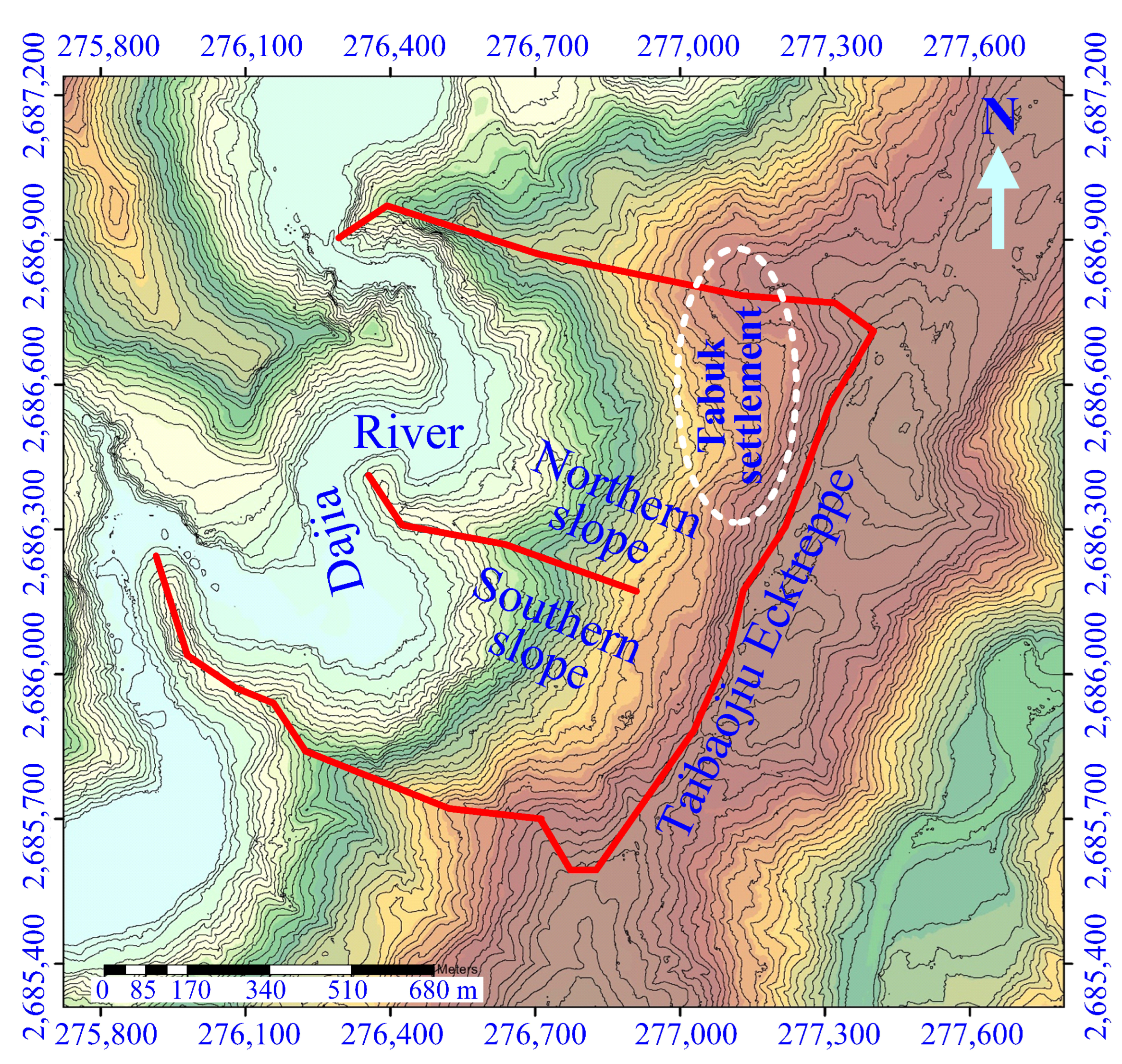
Topographically, the study area is located at the west wing of the Central Mountain Range, with elevations ranging between EL. +1420 m and EL. +1800 m; mountain and valley are the two main terrain features found in the study area (Figure 2). The northwest boundary of the study area is bounded by the Dajia River, which has a total length of about 120 km and flows from the northeast to the central west of the island of Taiwan, while two transmeridional ridges and the flat-topped Taibaojiu Ecktreppe (Figure 2), respectively, bound the northern, southern, and eastern boundaries of the study’s large-scale slope. A third transmeridional ridge divides the study area into the northern and southern slopes (Figure 2), making the main topography of the study site look like a pair of “dustpans” with their lip facing the Dajia River. Meanders, alluvial fans, and river terraces are common topographies found along the river. The overall topography of the study area is high in the east and low in the west, where the northern and southern slopes both dip to the west with slope angles ranging between 15 and 30 down to the Dajia River. The terrain stretching between the highest point of the Taibaojiu ridgeline and the lowest point of Dajia River Valley is steep–gentle–steep.
2.2. Temperature and Rainfall
Located at an altitude of EL. +1420 m and above, the study area attracts an average annual temperature of 15.2 °C. The lowest and highest average monthly temperature is 9.4 °C in January and 23 °C in July, respectively. The average annual rainfall between 1971 and 2016 was about 2215 mm, with a maximum average annual rainfall of 3771 mm in 2005. Table 1 shows the monthly and yearly average and maximum rainfalls recorded between 1971 and 2016, in which almost 70% of the 2215 mm average annual rainfall occurred between April and September; the month with the highest average monthly rainfall was June, which exceeds 300 mm. The huge discrepancy between the monthly average and the maximum rainfall during the recorded period was due to the extreme weather, which resulted in the uneven distribution of the rainfall [9].
2.3. Geology
Geologically, the study area is situated in the colluvial formation originally from the Miocene slate formation, and because of the frequent dynamic tectonic activities along with the high precipitation, the surficial slate of the study area has been found to be highly weathered [10]. The rocks stratum in the study area is dominated by the Lishan formation, also of the Miocene period, which comprises mostly slate and argillite with mature foliations, i.e., cleavage or schistosity [11]. Slate is characterized by rich foliations along which it breaks to leave smooth and flat surfaces. Because it is closely related to the axial planes of folds in the rock, it is often called the axial plane cleavage [11]. The orientation of the foliations of the slaty outcrop within the study area varies considerably. The main foliation fabrics, which were induced by the horizontal northwest–southeast compression, are sub-vertical, trending northeast–southwest at high angles. On one hand, slaty foliations with a high dip angle together with overturned and crooked foliations have been found along the river bank; on the other hand, broken slaty rocks with a gentle foliations orientation have been discovered at the higher elevations. Because the rock quality and weathering resistance of the slate with rich foliations are relatively poor, erosion has been a major concern and it has resulted in a relatively wide river valley. Lin et al. [12] have pointed out another concern whereby metamorphic rock slopes with well-developed foliations tend to creep under gravity with considerable variation in the orientations of the foliation, in compliance with the definition of a deep-seated gravitational slope deformation.
At the crest of the northern and southern slopes is the Taibaojiu Ecktreppe (Figure 2), which was formed by the action of the Nanhu and Hehuan creeks further west; its elevation range is between 1500 and 1900 m, which is the typical elevation for the Ecktreppe topography. Alluvial was found on the surface of its topography, indicating that the Ecktreppe was once the river-bed of a stream [13]. In the Dajia River at the toe of the northern and southern slopes, sedimentary rocks with clear patterns could be easily found.
2.4. Google Earth Images Taken between 2006 and 2018
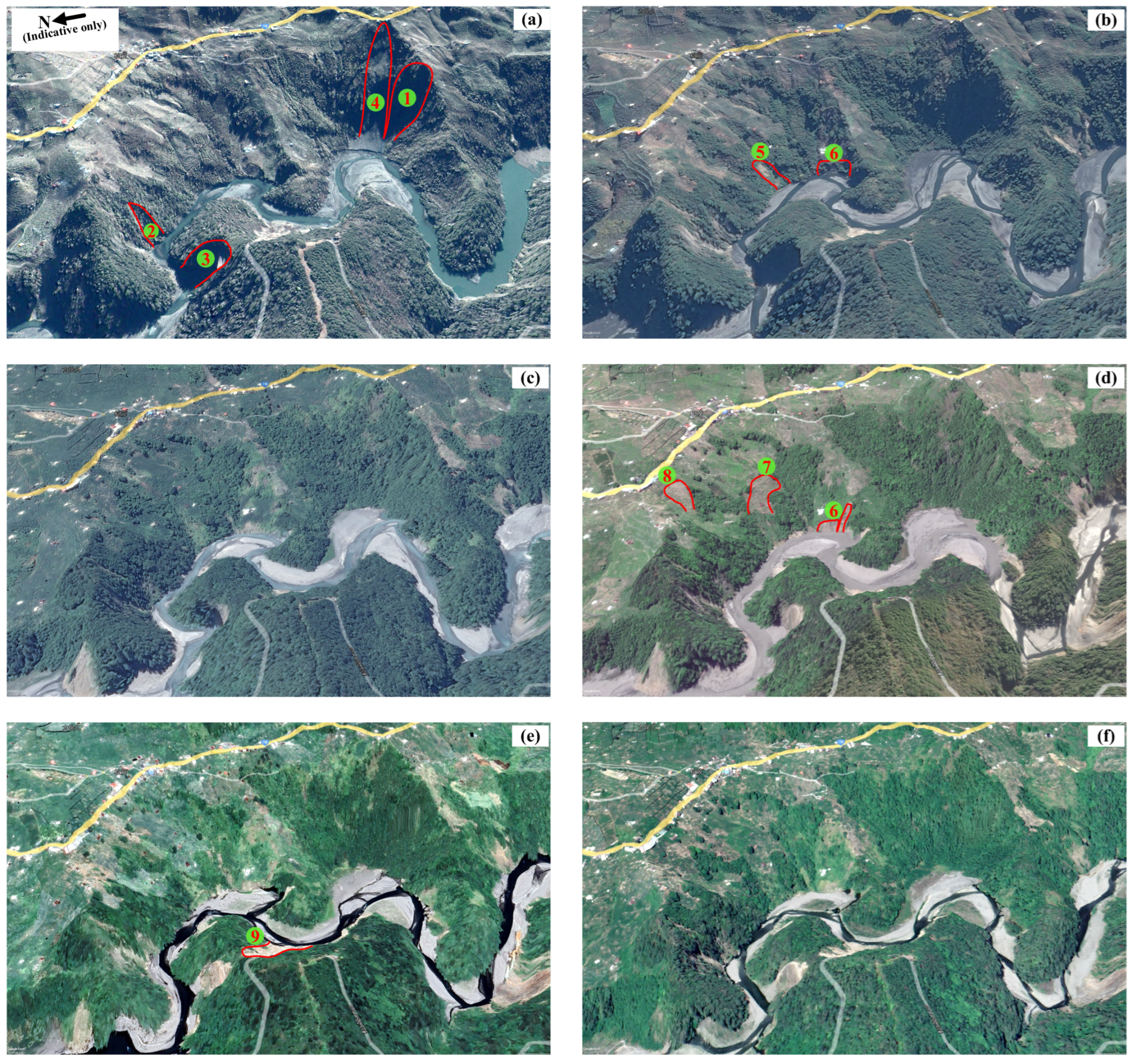
Six historical Google Earth [14] satellite images of the study area shot between 2006 and 2021 are presented and compared in Figure 3. Although the interpretation of satellite images, such as minor terrain variations, may be affected by the vegetation in the study area, the exposed surfaces as a result of slope collapses could still be identified in normal circumstances. The majority of the landslides have a visible rupture surface, main scarp, scarp floor, and deposition fan depositing most of the landslide debris; however, for open slopes, the deposition fan may not be available because the sliding debris could well be deposited on the trail path [15]. Perhaps the most obvious changes observed from these images are the headward erosion of the two concave banks of the northern and southern slopes.
Figure 3 reveals that the most distinct variation in the study site between 2006 and 2021 was the amount of water in the river and the transformation of the river banks due to erosion. Figure 3a shows the collapse of two river banks at locations Nos. 1 and 2 of the convex bank of the southern and northern slopes, respectively, and one collapse at location No. 3 of the concave bank opposite the northern convex bank. These collapses occurred as early as 2001, during which the river channel still had a considerable amount of water. On July 11 of 2004, a rather huge landslide occurred at location No. 4 of the southern slope, where the highest part of the main scarp of the landslide reached Provincial Highway No. 7A. Prior to November 2013, most likely in early 2012, two new failures were observed at locations Nos. 5 and 6 of the convex bank of the northern slope (Figure 3b), in which failure No. 5 was a shallow slope failure, whereas failure No. 6 was a cut bank failure. No new failures were observed prior to July 2016, as inferred from Figure 3c; however, surface erosion could be seen at locations Nos. 7 and 8 of Figure 3d while the collapse of the cut bank at location No. 6 was extended further. A failure at location No. 9 of the concave bank opposite the northern slope was reported some time in 2017 (Figure 3e). These collapses have been found to be closely related to the rainfall event associated with the various typhoons, as tabulated in Table 2. In general, the satellite images revealed that most of the slope collapses observed along this portion of Dajia River occurred along the two convex banks as the banks were easily subjected to fluvial attack and erosion. The critically eroding banks collapsed when an external factor, such as a high-intensity rainfall, disturbed their already fragile stability.
3. Methods of Study
The main methods used in this study consist of ground investigation via a series of boreholes and electrical resistivity tomography (ERT), slope monitoring that included monitoring the depth of ground-water level and the lateral displacement of the slope, and slope stability analysis that took into account the influence of a designed storm for 50-year return period in 24 h.
3.1. Ground Investigations
3.1.1. Boreholes Exploration
Ground investigation via a series of boreholes was conducted in this study to establish the soil and rock profiles and the materials parameters to be used in the stability analysis. Wire-line core drilling system with H-size drill rods and Q-group wire-line diamond drilling machine, which is associated with a core diameter of 63.5 mm and a hole diameter of 96 mm, was used for the exploration. The system is efficient in complete recovery of core from the rock mass without having to pull out the drill string.
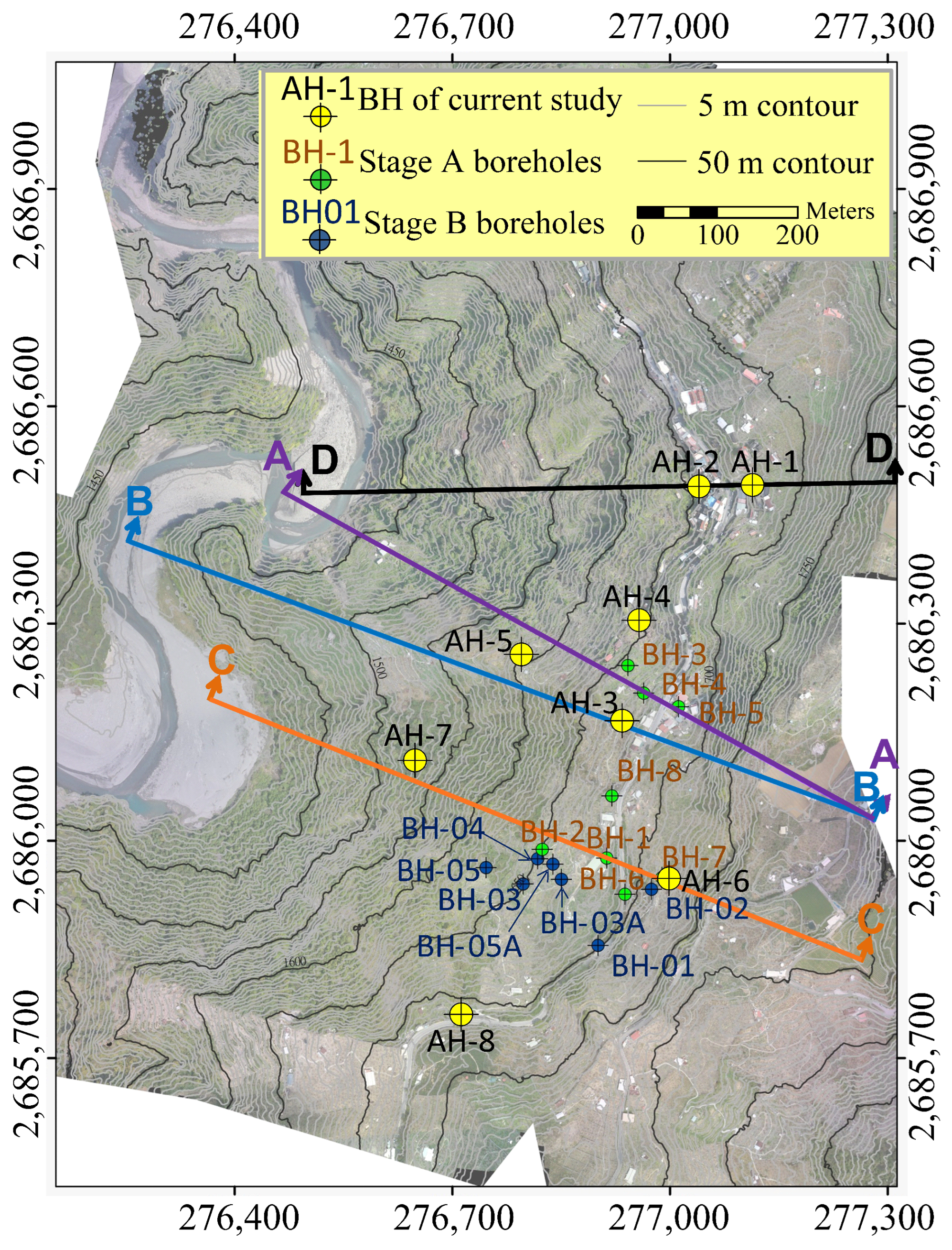
Prior to this study, some fourteen boreholes, which were mainly concentrated in the southern slope, were drilled by the Soil and Water Conservation Bureau in 2007 [9]. To realize the ground information of the transmeridional (central) ridge and that of the northern slope, additional boreholes were required. After a detailed on-site visual inspection, eight additional boreholes (AH–1 to AH–8) were assigned, as shown in Figure 4, and drilled in 2017. The depth of these additional boreholes, except AH–6 and AH–8, was 50 m; AH–6 was 60 m, while AH–8 was 40 m deep.
3.1.2. Electrical Resistivity Tomography (ERT)
As a near-surface geophysical tool, the ERT, which computes the below-ground distribution of electrical resistivity from a series of electrical resistance measurements, is a widely used geophysical subsurface imaging technique for providing information of geologic site conditions, hydro-geologic characteristics, environmental-related conductivity variability, etc. [16]. Because ERT is a rather advanced site investigation technique, the principle behind the technique is briefly described here.
How difficult it is for an electrical current to pass through a material is described by its electrical resistance R, where loose soil or a void in the ground will have a higher resistance reading, while compacted soil or a buried metal will have a lower resistance reading. Thus, when an electrical current I is generated in the ground, the electrical voltage V varies depending on the state or condition of the ground and, hence, the resistance R; according to Ohm’s Law (), R is expressed as the ratio of the measured voltage and current, but it varies with material’s volume. For an object with a length L and an area A, R is given by:
where is a constant of proportionality, also called the electrical resistivity or the specific resistance []. The reciprocal of electrical resistivity is conductivity, which represents a material’s ability to conduct electrical current and is often used as a representation of bulk property of earth material.
Unlike electrical resistance R, which varies with a material’s volume, electrical resistivity is a bulk property of a material and it has the same value for all lumps of that material, regardless of geometry. Thus, using either an alternating current (AC) or a direct current (DC), ERT can be used to measure the variations in electrical resistivity either at the ground surface or by electrodes installed at depth [17]. However, the value of resistivity is commonly affected by ground materials, minerals composition, particles size, and salinity of water.
From Ohm’s Law and taking the surface area A of a hemisphere with a radius r as and the length , one may derive the electrical potential or voltage V as
where I is the electric current in amperes, which flows radially away from the current source along the ground surface; hence, the potential V varies inversely with distance r from the current electrode.
The voltage, or, more precisely, the potential difference over a homogeneous half-space with a four-electrode array (Figure 5), is given by:
where and are the electrical potentials at and and is the distance between electrodes and , etc.
In practice, resistivity surveys are normally performed over inhomogeneous mediums where the subsurface resistivity has a 3-D distribution [18]; in this case, the measurements of the resistivity are still conducted by passing a current into the ground via the current electrodes and and recording the potential difference between the electrodes and . The apparent resistivity —defined as the resistivity of an electrically homogeneous and isotropic half-space—is related to the applied current I and the measured value of potential difference for a given arrangement and spacing of electrodes as [18]
where k is a geometric factor that is governed by the arrangement of the four electrodes; k in Equation (4) is found to be
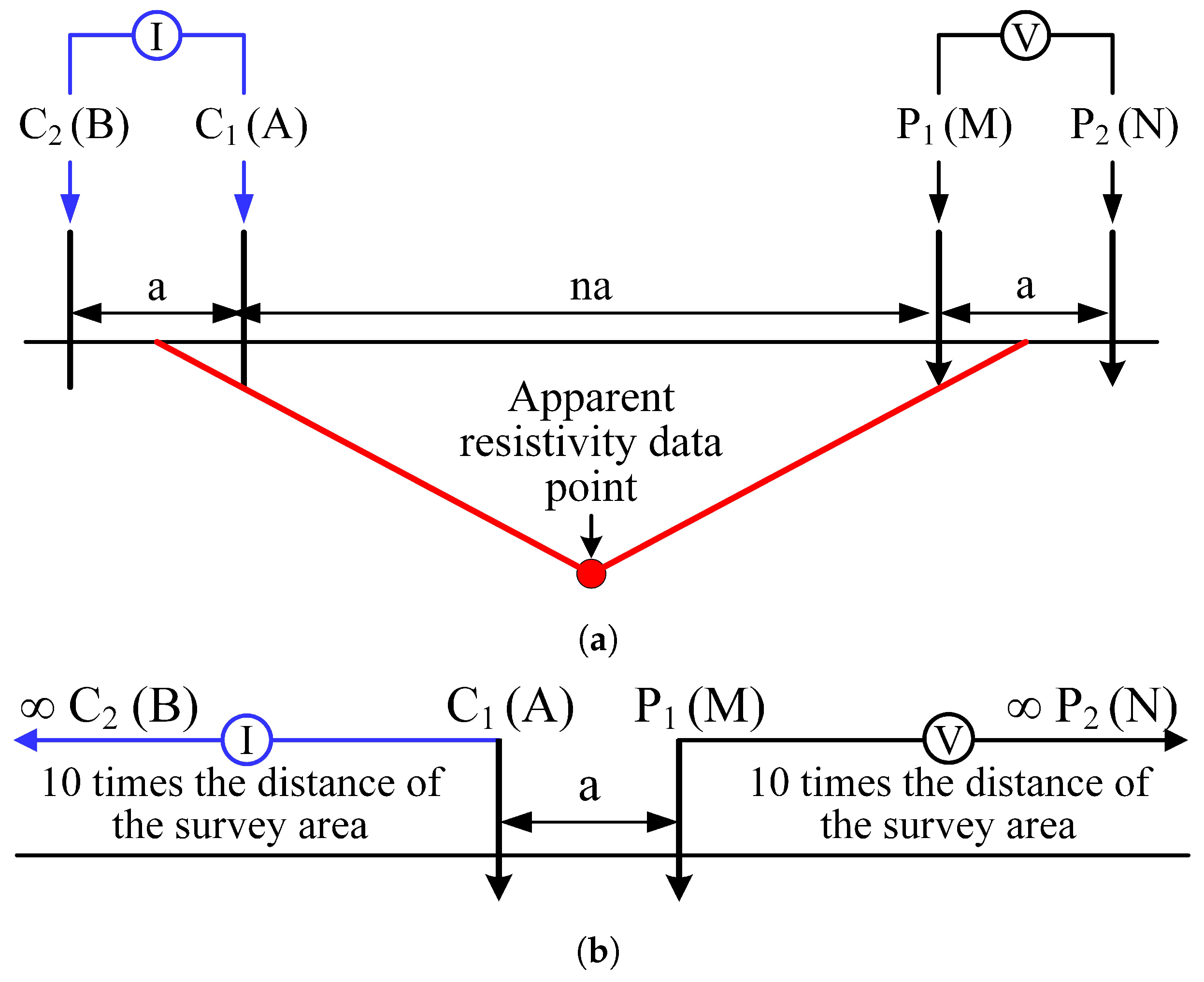
Two types of electrode arrays were deployed in this study: the Wenner–Schlumberger array, Figure 5a, and the pole–pole array, Figure 5b. On one hand, in the Wenner–Schlumberger array, the distance between the current and potential electrodes (or ) was “n” times the distance between the two potential electrodes pair . This arrangement allowed the detection of greater concentration of high resistivity values beneath the electrodes and [19]. The configuration of Wenner–Schlumberger array was reported to be moderately sensitive to changes in resistivity horizontally and vertically and, thus, it is suitable for areas with complex geological conditions [20].
The pole–pole array, on the other hand, is often used for deep imaging through the placement of two remote electrodes ( and ) at infinity, while the distance between the transmitter dipole and the receiver dipole was comparatively short [21]. Here, a single transmitting electrode is called a pole, while a pair of oppositely charged electrodes is called a dipole. The dipole is closely placed so that the electric field would seem to be a single electrode field instead of field from two different electric poles [21]. Quantitatively, to ensure a measurement error of less than 5%, the second current and potential electrodes ( and ) would have to be moved in the opposite direction and placed at a distance of at least 10 times the maximum distance between and electrodes; in other words, this array has a stationary infinity electrode on either side of the survey area, Figure 5b. “Super-Sting R8” multi-electrode resistivity system was used for geologic mapping in this study as it allows for rapid analysis of site conditions below the ground surface.
3.2. Field Monitoring
In addition to the boreholes exploration and electrical resistivity tomography, the water level and lateral deformation of the northern and southern slopes were also monitored by observing the water level via the observation wells and the inclinometers, respectively.
Observation Wells
Groundwater levels across a site may be determined via (i) groundwater observation wells; (ii) piezometers; (iii) open boreholes; and (iv) field estimates. For the study site, direct monitoring via observation wells and piezometers were used. The observation wells were mainly used to identify the shallow groundwater levels, while the piezometers were used to measure the piezometric head of the confined groundwater. Because the shallow groundwater levels are easily influenced by the rainfall and the rise in such water levels could result in slope instability, eight observation wells (AH–1 through AH–8) were drilled and installed next to the locations of the inclinometers for the direct monitoring of the groundwater levels in the study slopes, in particular during the rainy seasons in 2017. The groundwater levels in the wells were measured manually with a calibrated steel tape once a month; in addition, extra measurements were also taken when the 24-hour accumulated rainfall exceeded 400 mm.
3.3. Inclinometers
Monitoring stations for inclinometer are effective way of monitoring a landslide and detecting the associated sliding surface [22]. In total, five inclinometer points were installed, in which a 50 m long specially grooved casing was inserted into each of the existing boreholes, AH–2, AH–3, AH–4, AH–5, and AH–7. Cement grout was injected to fill the annular void; these boreholes were thus unsuitable for use as observation wells. The servo-accelerometer probe was lowered and raised through the specially grooved casing, which guides the movement of the probe within the casing via its four orthogonal longitudinal wheel grooves. Readings were taken manually once a month, and additional measurements were also taken when the 24-hour accumulated rainfall exceeded 400 mm.
3.4. Seepage and Stability Analyses
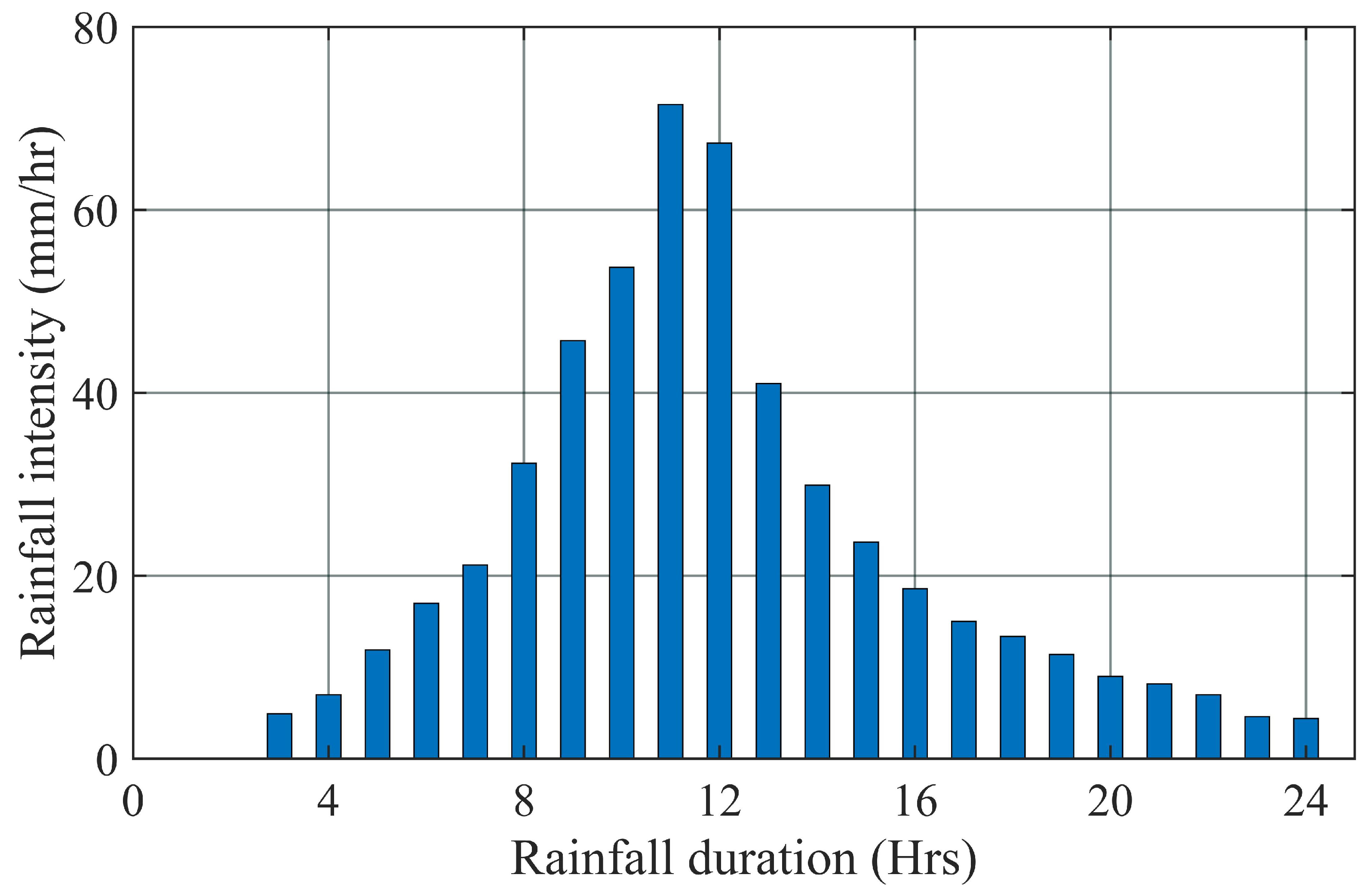
The stability of the northern and southern slopes may be assessed using conventional slope stability analysis, taking into consideration, in particular, the effect of short-term rainwater infiltration. The uncoupled hydromechanical stability analyses were performed using the program SEEP/W and SLOPE/W with a three-stage approach. Firstly, the steady-state seepage analysis, using the approach of variably saturated flow and the parameters listed in Table 3, was performed to obtain the hydrostatic pore-water pressure distribution in the slopes. Secondly, using the result from the first stage and the designed rainfall (Figure 6), a transient analysis was conducted to simulate the infiltration of rainwater and obtained the corresponding change in pore-water pressure distribution in the slopes; this was followed by assessing the stability of the slopes based upon the shear strength parameters given in Table 3 and the distribution of pore-water pressure obtained from the above transient analysis. In Table 3, the parameters: saturated and residual volumetric water content, a, and n were the fitting parameters for the corresponding van Genuchten’s [23] soil–water characteristic curve (SWCC) and hydraulic conductivity functions; another fitting parameter m was taken as .
It should be emphasized that uncoupled analysis is by no means perfect. Firstly, for rainfall infiltration-related analysis, Khoei and Mohammad [24] and Airey and Ghorbani [25] recommended that coupled or fully coupled models should be preferably used because deformation of solid significantly affected its pore air and water pressures. Secondly, the van Genuchten’s SWCC and hydraulic conductivity models adopted here were assumed to work under constant void ratio or under conditions in which the material’s volume does not change appreciably, thus ignoring the effect of initial void ratio on air-entry value [26,27] and also the effect of hydraulic hysteresis [28], which are known to significantly affect the hydromechanical response of soils. In practice, because the problem of slope stability is inherently a large deformation problem, materials’ void ratio changes appreciably as a result of such deformation [29]; thus, for a more complete analysis, these two functions should be updated throughout the analysis. In addition, the effect of stress-induced anisotropy, which has always been a concern in problems related to slopes stability [30,31], is also not considered in this study. Nevertheless, they were commonly adopted in practice because of their availability and ease of use.
Based on the monitoring data collected between 1990 and 2016 from the nearby Tabuk rainfall station and the simple scaling Gauss–Markov analysis, the designed storm for 50-year return period in 24 h (Figure 6) was derived and used as the boundary condition in the transient analysis. The Morgenstern–Price method used in the stability analysis is one of the many general methods of slices formulated based on the principle of limit equilibrium; it satisfies both the equilibrium of forces and moments acting on individual blocks.
4. Results and Discussion
4.1. Ground Investigation Results
4.1.1. Slopes Materials
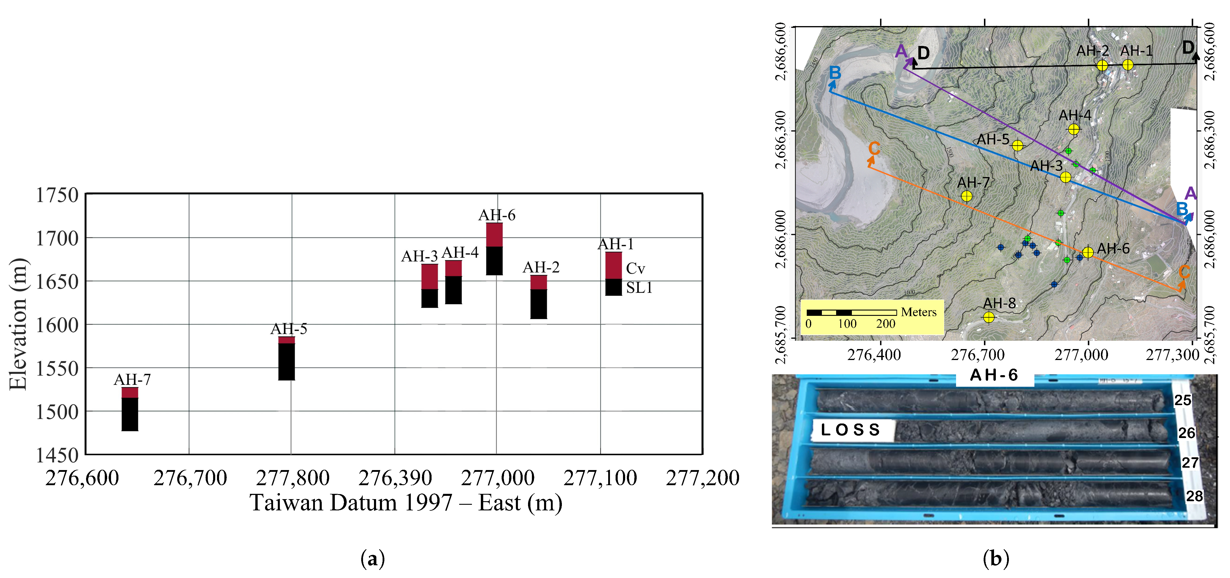
A general stratigraphy of the study site was derived from the analysis of the cores extracted from the seven boreholes drilled across the study site. The stratigraphy of each core and the location of the boreholes are presented in Figure 7.
From the boreholes cores analysis, it was found that colluvium (Cv) of varying thicknesses occupied the top layer of the slopes (Figure 7a). The colluvium consists of the yellowish brown to gray clayey silt, and sand with lightly to moderately weathered slate fragments, occasionally accompanied by slate debris with quartz detritus, but the engineering characteristic of this colluvium is dominated by the clayey silt and sand. The Standard Penetration Test (SPT) “N” values ranged between 2 and 20, but sometimes they could be as high as 40. The thickness of the colluvium varies considerably, with a maximum thickness of 31.3 m at borehole AH–1.
Beneath the colluvium was the gray to dark gray slate of fair rock mass quality, occasionally with a quartz vein. The disintegrated and fragmented rock materials found here were mainly due to the weathering process. The slaty cleavage (SL1) has a gentle dip of between 10 and 30 and a gouge was found present in this clastic rock mass, indicating that the fissures of the flexural toppling slate were well-developed and hence induced relative displacement under the long-term gravitational force; consequently, SL1 is continuously under creeping and slipping.
The third layer was basically formed by the anti-dip (obsequent) and high-angle foliations slate (SL2) [32]. Under normal circumstances, obsequent slate slopes with high-angle foliations would normally cause the deformation of flexural toppling, the formation of bending folds in the upper slope, and rock falling [11]. However, this should not be the case for the study site because only a small portion of the rock mass toward the toe of the slope of section B–B and section C–C (Figure 7b) exhibits such day-lighting foliations; the anti-dip slate with high-angle foliations in the other two cross-sections were not day-lighting and thus their tendency to toppling is being refrained by the overlying colluvium.
Finally, a total of 34 soil samples—selected from a total of 360 m long cores recovered from the boreholes—were tested in a geotechnical laboratory for the determination of their physical properties and shear strength. The result of the laboratory tests are tabulated in Table 3, and they were used in the following seepage and stability analyses.
The ERT survey results of the Wenner–Schlumberger and the pole–pole arrays for cross-sections ERT1 (Section B–B in Figure 4b) and ERT2 (Section C–C in Figure 4c) are plotted in Figure 8. The ground layers inferred from the borehole cores analysis are also shown in this figure.
The resistivity readings obtained from both the Wenner–Schlumberger and pole–pole arrays for the northern and southern slopes ranged between 100 and 500 m. The variation in the resistivity reading is more discernible and unevenly distributed near the ground surface than that at a deeper depth. Care must be taken when interpreting the resistivity readings for the following reasons: (i) it is possible for a particular material to have a wide range of resistivity readings as a result of its saturation degree, ions concentration, faulting, jointing, weathering degree, etc., (ii) most of the resistivity reading of the near-surface sedimentary materials is mainly dictated by the amount and the chemical contents of their pore water, and (iii) clayey soils and sulphide minerals are the only sedimentary materials that allowed an enormous amount of electrical current passing through themselves [33].
The resistivity reading variation in Figure 8 was expected as the resistivity measurements in the slate formation were dictated by the presence of water in the rock fissures and the relative degree of the shear fracture and shear gouges; however, in the colluvium, the degree of moisture content, fine content, and rock-fragment content were the known factors that governed the resistivity measurement. The borehole sampling revealed that the fine content of the colluvium was higher than that of the slate; the overall resistivity reading of the colluvium in the two cross-sections was thus lower than that of the loose colluvium or with fragmented rock where the resistivity value was higher.
Core samples from the site investigation revealed that the orientation of the disturbed slate foliation SL1 was almost horizontal or gently plunging, and the disturbed slate SL1 consisted of poor quality rock masses, often filled with gouges of varying thicknesses. The resistivity measurements of the slate converged with a depth to about 200+ m, indicating that within the investigation depth the resistivity measurement was still governed by the fine content of the slate and the in situ pore water. An intriguing pattern of resistivity distribution was observed from the results of the Wenner–Schlumberger and pole–pole arrays. Unlike the low resistivity-based colluvium that occasionally mingled with some high resistivity reading, a higher resistivity reading was measured near the ground surface of the ERT-1 survey line between 0K+110 and 0K+230 m, Figure 8c; after re-visiting the site, it was found that said location was in fact covered by slate with gently plunging foliation. A similar phenomenon was also seen between 0K+00 and 0K+20 m of the ERT-2 survey line where the steep slope is located, Figure 8d. A further study can be performed in the future to examine whether the method is suitable to be used to deduce the degree of bending and toppling of the foliated rock mass under gravitational force.
The interface between the colluvium (Cv) and the disturbed slate formation (SL1) was postulated and is plotted in Figure 8 using the white dotted line. The interface was deduced from the results of the ERT survey, borehole coring, and outcrops noted from the study site. The postulated interface revealed that the thickest colluvium was located in the vicinity of Borehole AH-3 on the ERT-1 survey line, while that on the ERT-2 survey line was roughly located between 0K+300 m and 0K+500 m.
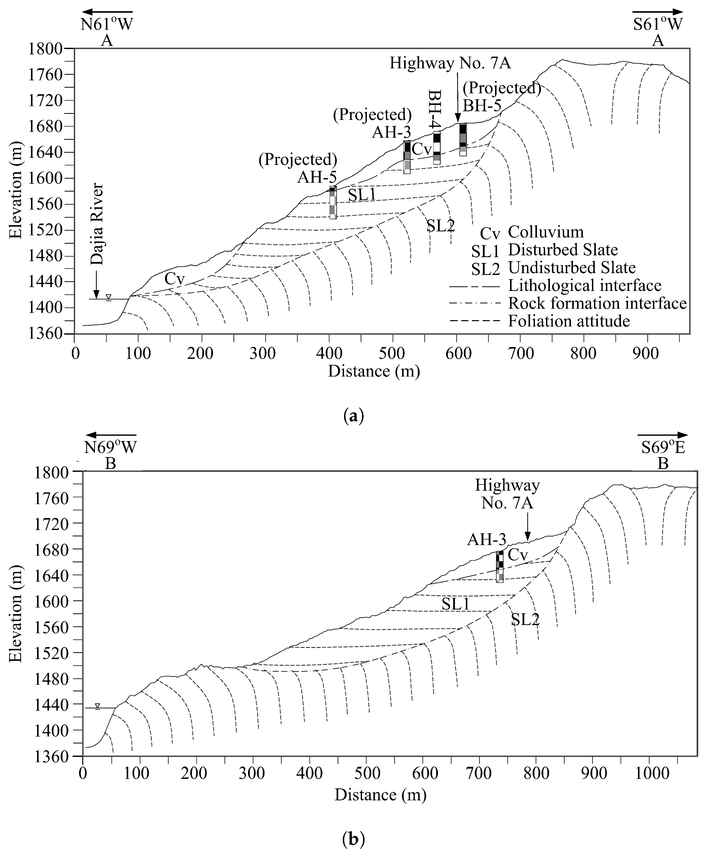
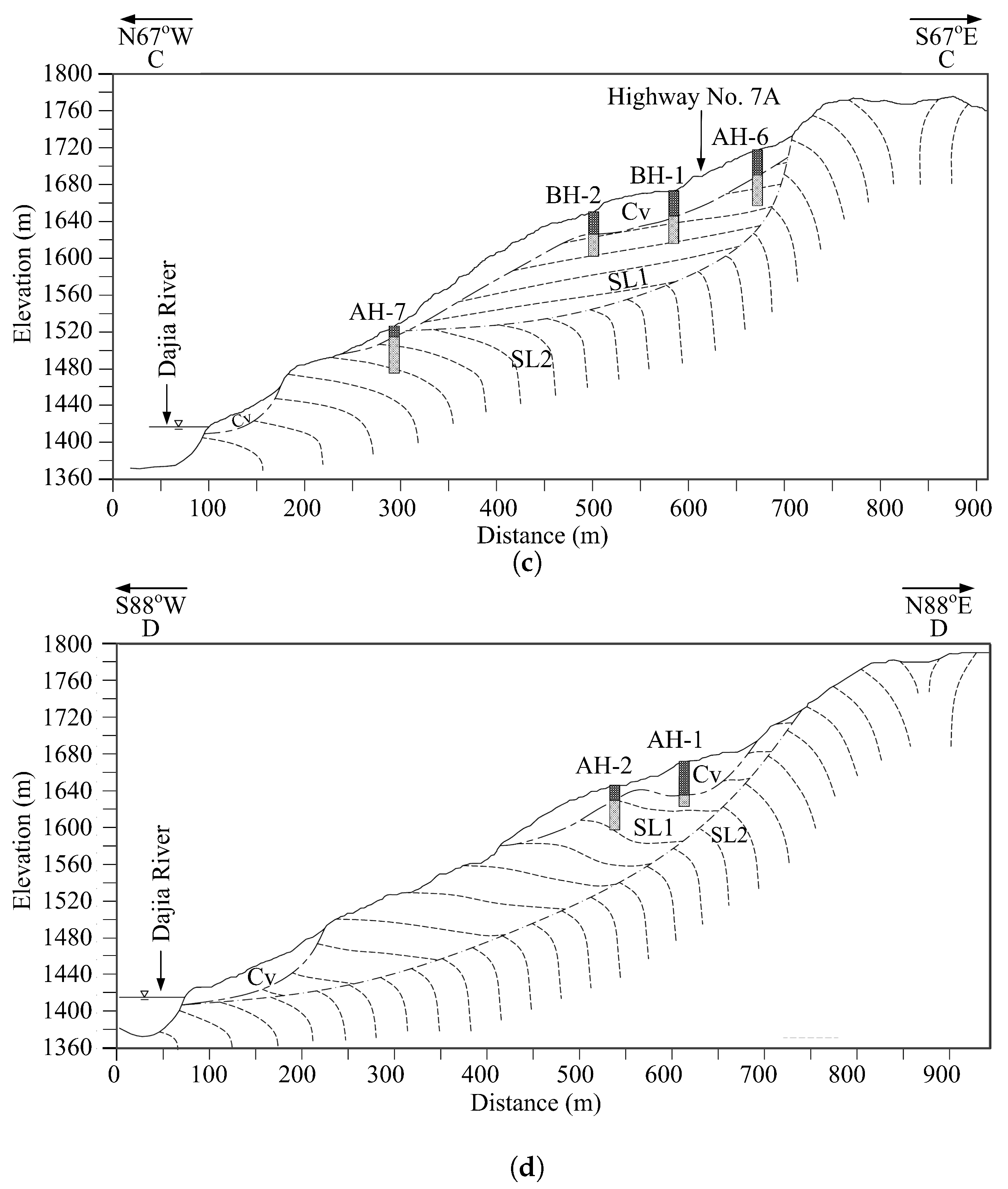
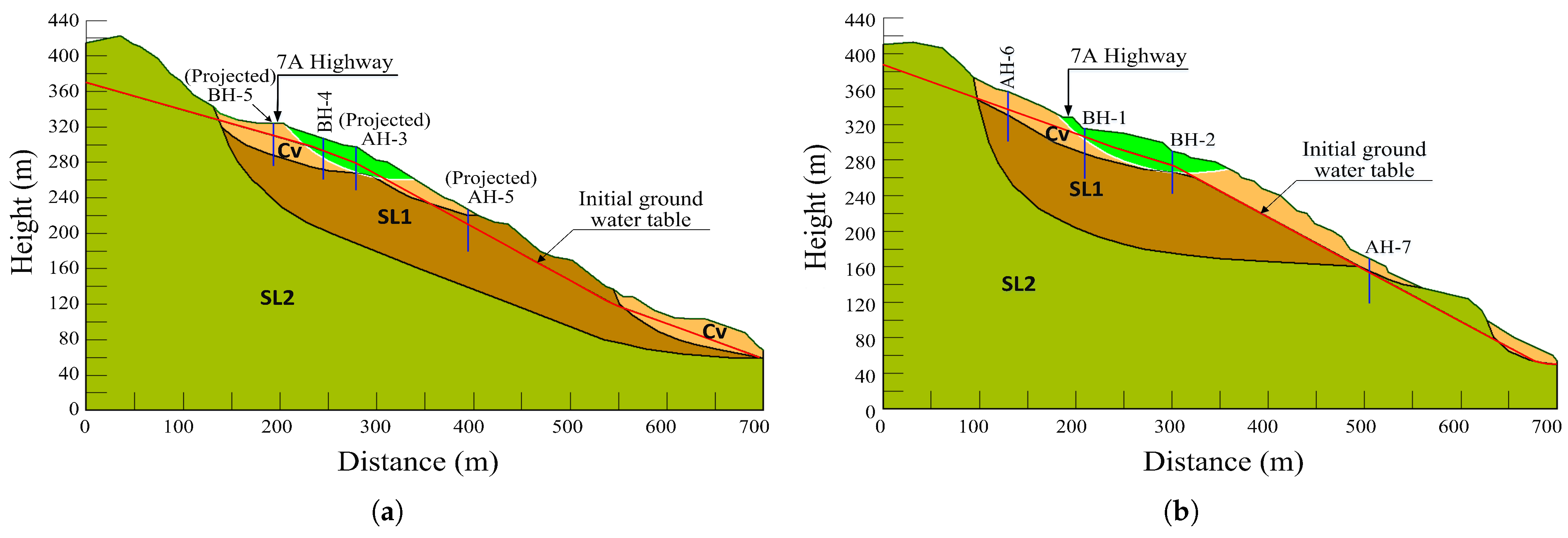
Finally, the stratigraphic layout for each of the four designated cross-sections, as shown in Figure 4, is plotted in Figure 9; these layouts were deduced via the combination of the desk study, the subsurface geologic mapping, and the borehole cores analysis, as presented above. However, due to the limited number of boreholes, the stratigraphic layouts derived here may be oversimplified; to quantify the error associated with such a simplification, the Boolean Stochastic Generation approach, as proposed by Bossi et al. [34], may be adopted. Nonetheless, such a comprehensive analysis is out of the scope of the current study.
4.1.2. Groundwater Level of Study Slopes
The highest groundwater level in each observation well recorded for the study site is tabulated in Table 4. The results show that the highest groundwater level was located either in the colluvium layer or in the vicinity of the interface between the colluvium and the slate formation (SL1).
4.1.3. Lateral Displacement of Slopes
The installation of the inclinometers AH–3, AH–4, and AH–7 (Figure 4) was completed on June 11, 2017, while that of AH–2 and AH–5 was completed on August 16. Thus, only the records of AH–3, AH–4, and AH–7 are presented here in Figure 10. The inclinometer AH–3 was originally 50 m long, but it was found broken at a depth of 27.5 m in a local sliding event just after installation (Figure 10), and continuous displacement was observed at depths between 24.5 and 27.5 m. Coincidentally, the thickness of the colluvium at AH–3, according to the borehole log, was about 29.2 m, and the large inclinometer or shear displacement reading at the depths between 24.5 m and 27.5 m revealed that the sliding surface, induced by the extreme rainfall, was located within the colluvium layer. In addition, the sliding thickness could be as deep as the thickness of the colluvium because the disturbed (SL1) and undisturbed (SL2) slate formations could both be regarded as relatively stable strata. Within the period of monitoring, no obvious displacement and trend of movement were observed in the inclinometers AH–4 and AH–7 (Figure 10) as their readings were within the measurement margin of error. According to Machan and Bennett [35], the field accuracy of an inclinometer is roughly ±7.6 mm per 30 m, which includes a combination of random and systematic errors. The random errors occurred within the sensors and affected the accuracy of the inclinometer probe, while systematic errors occurred because of human operations and influenced the condition of the probe and the procedure of data collection [35]. No further measurements were taken for the inclinometers AH–4 and AH–7 in the subsequent months because of the discontinuation of the project.
4.2. Factors Causing Short-Term Sliding
The three main factors, (1) the infiltration of rainwater on the slope, (2) upraised river-bed elevation caused by earthquakes and seasonal typhoons at the toe of the slope, and (3) erosion of the river bank of the slope toe, were believed to be crucial in initiating the slope instability.
The result of the seepage and stability analyses revealed that prior to the rain (0∼2 h), the factor of safety (FOS) of the cross-section A–A of the northern slope and the cross-section C–C of the southern slope was 1.04 and 1.22, respectively. The FOS of the slopes was then re-assessed for every subsequent hour of infiltration. It was found that the FOS of the cross-section A–A of the northern slope decreased to 1.00 after 14 h of rainfall and to 0.98 at the end of 24 h. Likewise, for the cross-section C–C of the southern slope, its FOS decreased to 1.00 after 18 h of rainfall and to 0.98 at the end of 24 h of rain. The corresponding sliding zone for both the analyzed cross-sections at the end of 24 h rainfall is plotted in Figure 11. As seen from this figure, both sliding zones were located in the top half of the slopes and extended to Provincial Highway No. 7A. The colluvium deposit located at the toe of the study slopes (Figure 9) is believed to be the debris produced as a result of the local failure of the overlying colluvium of the up-slope. The deposit at the toe of the slopes subsequently led to the rise in the groundwater level and triggered the instability at the toe of the slopes. The projected location of the inclinometer AH–3 was included in Figure 11a, which shows the analyzed sliding surface of the cross-section A–A; the depth of the sliding surface given by the simulation was about 28 m deep, which was very close to the depth at which the inclinometer AH–3 was found broken, i.e., at 27.5 m.
The slope collapses reported in Section 2.4 were mainly due to the rise in the river-bed and the erosion of the river bank or slope toe. The study area is located at the upstream of Deji Reservoir and the sedimentation produced by the erosion further upstream has resulted in the rise in the elevation of the river-bed of the study area. According to local residents, the condition of Dajia River has been deteriorating since after the construction of the Deji Dam in 1973 as a result of the severe river-bed sedimentation, especially in the early 2000s. The 921-Jiji earthquake resulted in the elevation of the river-bed rising by 10 m; in 2001, the river-bed elevation rose by 8 m around the period when Typhoon Toranji ripped past the island; in July 2004, Typhoon Mindulle caused the river-bed to rise by a further 10 m; and a month later, on 25 August 2004, Typhoon Aere pounded northern Taiwan with torrential rains and increased the elevation of the river-bed by another 6 m. Thus, within a period of five years, the elevation of the river-bed of Dajia River was raised by some 34 m while the width of the river was doubled. The consequent increase in the river-bed elevation changed the topography of the slopes and eventually affected the movement characteristics of the slope.
In addition to the uprise in the river-bed elevation, the erosion of the outer-bank (cut bank) of the meandering, as discussed in Section 2.4, is another destabilizing factor of the northern and southern slopes. Because the toe of the southern and northern slopes ended at the concave cut bank, the current of Dajia River was continuously eroding and steepening the toe of the slopes and increasing the tangential component of the disturbing force, thereby reducing the stability of the toe of the slopes. Furthermore, rain accumulated within the ridge-top depression at the slope crest, infiltrated into the slope, and eventually seeped out from the surface of the toe of the slopes or river bank before entering into the Dajia River; the seepage force along the sloping direction together with the gravitational force caused the slope to be susceptible to instability. Another possible reason could be due to the excess pore-water pressure generated in the saturated bank, which reduces the shear strength of the river bank and increases the sliding force and, in turn, contributed to the instability of the slopes.
4.3. Factors Causing Long-Term Sliding
The result of the ground investigation and geophysics tests of the study area showed that the slopes were basically formed by disturbed slate (SL1), undisturbed slate (SL2), and occasionally by the overlying of wedges of colluvium deposit on the surface (Figure 9). The slate outcrops within the study site revealed considerable variations in the foliation orientation. The foliations of the SL2 slate of the bank of Dajia River and that toward the toe of the slopes are found bowing down-slope, while the foliations of the SL1 slate are oriented nearly horizontally. These down-slope bowing (toppling) foliations were induced by the long-term down-slope gravitational force and they could lead to the formation of a bending fold [36]. The SL1 slate was seriously disturbed during the process of the right-angle curving or bending of its foliations into the gently dipping or horizontal foliation; it is thus unsurprising to observe on site that SL1 is of a poorly integrated rock mass compared to the more intact SL2 rock mass.
At the crest of the slope, at an elevation of about 1784 m, is the Taibaojiu Ecktreppe. Figure 4 reveals that the landform of the Ecktreppe has somehow crept into a double-crested ridge or ridge-top depression; in other words, the crest crept westward toward the Dajia River and eastward toward the Hehuan Valley. The phenomena is consistent with the criteria and structural landform induced by a large-scale deep-seated gravitational slope deformation (DSGSD), which is driven by the process of mass rock creep (MRC) [37]. In studying the long-term gravitational deformation of rocks slopes, Chigira [36] concluded that when the subsurface rocks of the slopes are continuously subjected to an unstable state under the influence of gravitational force, the subsurface rocks deformed to various degrees in various ways by means of MRC. The disturbed rock mass SL1 is believed to be creeping at a very slow rate. Although the creeping rate cannot be detected over a short period of time and the modes of movements are not always evident, creeping may still bring gradual but continuous damages to the slopes [36].
Chigira [36] categorized the macroscopic deformational structures of the MRC into Types I∼IV folds that changed according to the relationships between foliations and slopes. Using the classification of the attitude of foliations defined by Chigira [36], the MRC structure of the exposed down-slope bowing foliated rock mass of the northern and southern slopes shown in Sections B–B and C–C of Figure 9 would be categorized as Type III folds. According to Chigira [36], this type of fold often led to small debris avalanches by means of the valley-ward bulging of a fragmented rock mass, and such a phenomenon revealed the inherent danger of the northern and southern slopes as it could occasionally trigger huge and catastrophic landslides.
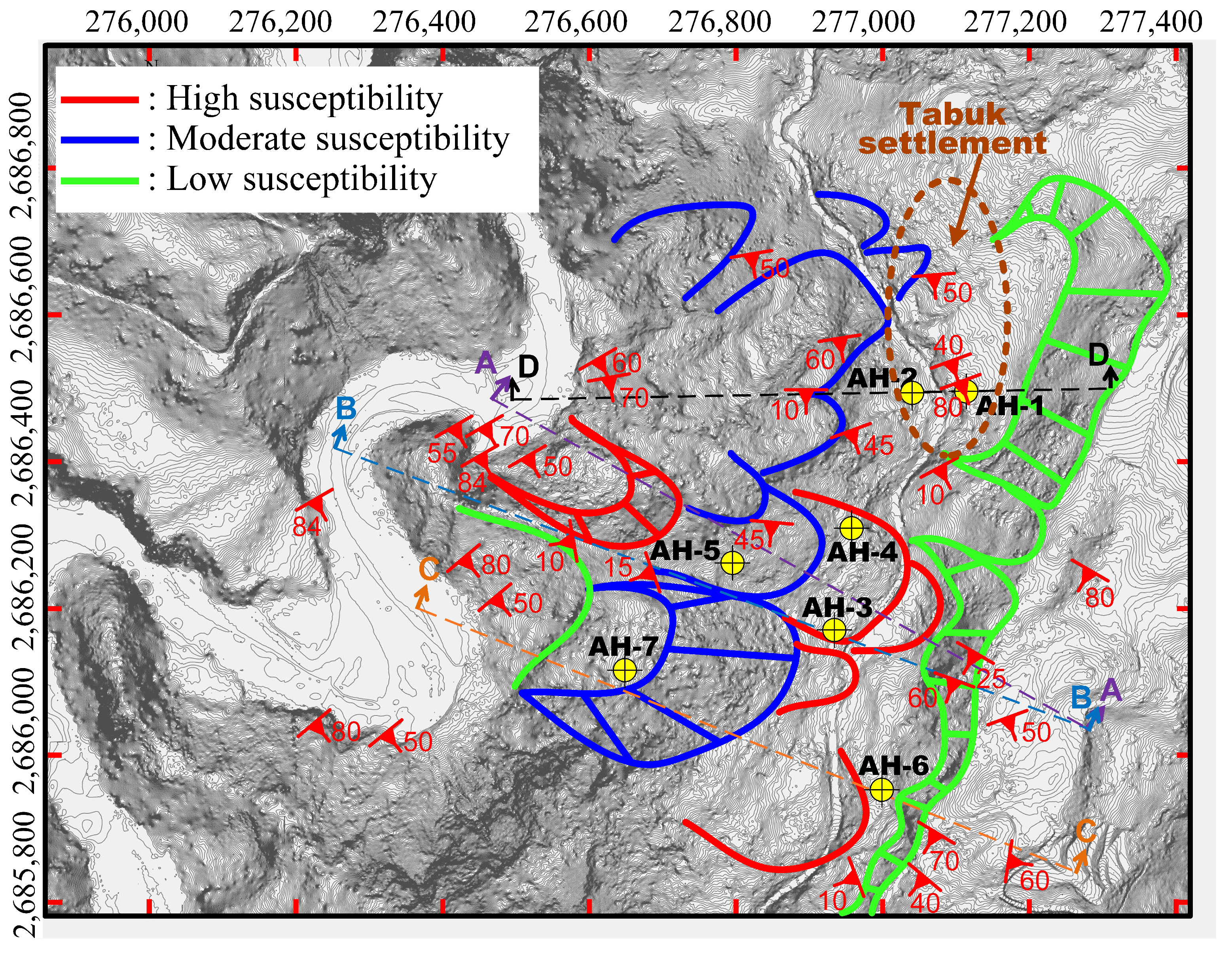
A sliding susceptibility assessment was carried out for the study site. The dip direction of the slate is plotted together with the sliding susceptibility zones in Figure 12. In general, the slate around the toe of the slopes and the river valley dipped more steeply than that of the two slopes. The strike and dip measurements of the slate at the toe of the slopes and the river valley were more reliable than that of the slopes because the slate at these two locations is mainly undisturbed, while the measurements on the slopes were made on the slates that were disturbed by DSGSD and, in particular, the local sliding to varying degrees. An individual potential sliding body on the study site was interpreted based on the topography features such as the slope gradient and slope aspect, which can be clearly interpreted from the Digital Terrain Model (DTM), in this case, with a contour interval of 1 m. Kasahara et al. [38] used satellite and Google Earth imagery and a visual inspection to produce a landslide susceptibility map with respect to land use. In this study, the Google Earth imagery was cross-examined with that from the aerial photographs taken on 23 August 2014, the Unmanned Aerial Vehicle (UAV) imagery taken on 19 April 2017, and field checking; it was decided to classify the sliding susceptibility of the study site into three categories, low, moderate, and high susceptibility, as shown in Figure 12. The sliding susceptibility classification was made based on the following evaluation:
- High susceptibility (red): Evidence of sliding, such as sliding surfaces, indicated by monitoring instruments, new cracks, ground subsidence, or broken drainage ditches within the sliding body, was found during field checking.
- Moderate susceptibility (blue): No evidence of sliding was found; however, signs of impending sliding, such as scarp, tilted ground, old cracks, and colluvium deposits, were observed during field checking.
- Low susceptibility (green): No obvious signs of soil slippage were seen during the field checking but could be inferred from topography features.
It can be seen that most of the potential sliding zones, in particular the high susceptibility zones, are concentrated on the central transmeridional ridge that divided the study area into the northern and southern slopes. There was a high sliding susceptibility zone at the bottom half of the northern slope, which happened to have colluvium as its surface soil and the river bank at its toe; according to the finding of Zhong et al. [39], although the slope gradient was not high, it was still prone to rainfall-induced accumulation failure in which the failure would be initiated from the toe of the slope. The Tabuk Indigenous settlement that this study is concerned with is exposed to a moderate sliding susceptibility.
4.4. Hazard Mitigation
Intense rainfall and infiltration: The subsequent rise in the groundwater level above the almost impermeable rock strata that prevented the groundwater from infiltrating downward and the upraised elevation of the river-bed of Dajia River together with the erosion of the river bank were the main destabilizing factors of the northern and southern slopes. A two-stage mitigation method is proposed for the study site. Firstly, the source for the rising groundwater or the infiltration of the rain into the ground has to be reduced quickly by means of surface drainage; secondly, the raised groundwater level has to be quickly drained off by underground drainage.
Surface drainage is effective in preventing surface erosion, intercepting run-off, and reducing rain infiltration into the colluvium and the cracks of the fissure of the study slopes. A man-made surface or open ditches together with Dajia River at the toe of the slopes seemed to be an ideal surface drainage system of the study site. The flexible and low-cost ditches could work very well in the hilly environment as the environment fulfilled the minimum requirement for a ditch gradient of at least 2%; however, ditches should be lined to minimize the rain infiltration and erosion [40]. In addition, sufficient redundancies have to be provided in a surface drainage design to accommodate for blockage and uncertainties [41].
The use of underground drainage in preventing the rise in the groundwater level would indeed prevent the increase in the water content of the slopes, which would otherwise reduce the shear strength and, hence, the stability of the slopes. Generally, facilities such as the shallow depth (2 m < depth) subsurface blind ditches, horizontal drainage pipes, and water collection wells are used jointly to achieve the purpose of underground drainage. The successful mitigation of the Lishan large-scale landslide, which was about 8.5 km to the southeast of the study site (see Figure 1), involved the use of a subsurface drainage network that included 15 storm water drainage wells of 15 to 40 m in depth and 3.5 m in diameter [42], in which the drainage well was essentially a manhole structure designed to gather storm water. Thus, for this study, storm water collection wells would also be required to receive the infiltrated water from upstream collection via the horizontal drainage pipes that were connected directly through the walls of the wells. For efficient water collection, the horizontal drainage pipes connected to the wells should be arranged in such a way that they are spreading radially upward.
To discharge the groundwater quickly, the horizontal drainage pipes could be installed at a variety of depths. The horizontal drainage pipes in the shallower layer are applicable for a location where its groundwater level is within 3 m of the ground surface; pipes with a diameter of 50 mm to 62.5 mm should be installed at an upward inclination angle of 10 to 15. The deeper horizontal drainage pipes are suitable for a location where its groundwater level is deeper than 3 m; in this case, the pipes are installed at an inclination angle of 5 to 10, the diameter of the pipes varies with the geological conditions but is normally between 75 and 125 mm, and the maximum length of the pipes should be less than 100 m.
It is believed that surface drainage together with the underground drainage system of horizontal drainage pipes and collection wells could rapidly discharge the surface run-off and groundwater and decrease the rise in the groundwater level during a heavy storm. These measures could effectively enhance the stability of the northern and southern slopes.
As for the erosion problem of the two cut banks of the meandering, at first glance, single-row stabilizing piles seemed to be a good treatment in protecting the river bank. However, transporting the construction equipment to the required location is a particular concern because a paved access road is unavailable on the slopes and constructing even a temporary access road seems inconceivable as it would destroy the fruit farming on the slopes. It thus seemed that protecting the eroded slopes with a riprap wall using the material available locally is a more practical approach.
5. Conclusions
A study aimed at investigating the sliding susceptibility of a large-scale landslide-prone area on the west wing of the Central Mountain Range in central Taiwan where its crest houses an Indigenous settlement and Provincial Highway No. 7A has been conducted. Severe subsidence has caused a section of the Provincial Highway No. 7A to undergo road-bed differential settlement and damage to its retaining structures and drainage ditches. At the toe of the slope is Dajia River, which has also recorded several collapses along its river bank in the past. By accomplishing a series of multi-temporal satellite and aerial images comparisons, site investigations, ground monitoring, geophysics tests, and slope stability analyses, the following findings and conclusions have been made:
- It was astonishing to learn that the river-bed of the river at the toe of the studied large-scale slope has been raised by more than 30 m within a period of five years as a result of the inundation of debris from upstream after the construction of a dam downstream of the study site.
- The infiltration of rainwater from the surface of the slope, the upraised river-bed elevation, and the erosion of the river bank of the toe of the slopes have altered the landform and the groundwater level of the large-scale slope and eventually triggered several localized slope failures. The results of the uncoupled hydromechanical slope stability analysis where the analyzed slopes were subjected to a designed storm for a 50-year return period in 24 h revealed that a sliding surface was triggered within the depth of the colluvium. The thickness of the simulated sliding surface coincided with that observed on site.
- The landform of the Taibaojiu Ecktreppe at the crest of the study area has somehow crept into a double-crested ridge or ridge-top depression, indicating that the study area is being subjected to large-scale deep-seated gravitational slope deformation (DSGSD) by means of mass rock creep. Although the creeping rate has yet to be quantified, the study’s large-scale slope is believed to be creeping gradually. The orientation of the on-site foliations has also revealed the inherent danger of the northern and southern slopes in which huge and catastrophic landslides could eventually be triggered. Based on field monitoring records and the orientation of the foliations, the associated DSGSD surface was deduced to be developed along the interface of the disturbed (SL1) and undisturbed (SL2) slates.
- An intriguing pattern of resistivity distribution was observed from the results of the Wenner–Schlumberger and pole–pole arrays. Unlike low resistivity-based colluvium that occasionally mingled with some high resistivity readings, areas with a concentrated high resistivity reading were found to be associated with the orientation of the foliated rock mass. Further studies could be conducted to verify the reason for this association.
It should be noted that the SWCC and the hydraulic conductivity functions used in the simulation stated in Conclusion 2 have been assumed to work under a constant void ratio or conditions in which the material’s volume does not change appreciably. In practice, because the slope stability problem is inherently a large deformation problem, the materials’ void ratio changes appreciably as a result of such deformation [29]. Thus, for a more rigorous analysis, these two functions should be updated throughout the analysis. Nevertheless, the findings of this study would be valuable for formulating detailed countermeasures to protect and maintain the stability and safety of the Tabuk Indigenous settlement located at the crest of the study’s large-scale slope.
Author Contributions
Conceptualization, H.-A.C., C.-C.L. and M.-W.G.; analysis, H.-A.C., C.D., C.-C.L. and M.-W.G.; data curation, H.-A.C. and C.D.; writing—original draft preparation, H.-A.C. and C.D.; writing—review and editing, C.-C.L. and M.-W.G.; supervision, C.-C.L., S.-K.H. and M.-W.G. All authors have read and agreed to the published version of the manuscript.
Funding
A part of this study, (in particular, the ground investigation and field monitoring) was based upon the project SWCB-106-204 supported by Soil and Water Conservation Bureau.
Institutional Review Board Statement
Not applicable.
Informed Consent Statement
Not applicable.
Data Availability Statement
Not applicable.
Acknowledgments
We would like to thank the two anonymous reviewers for taking the time and effort necessary to review the manuscript and we sincerely appreciate all their insightful comments and suggestions, which helped us to improve the quality of the manuscript immensely. We are also grateful to Director-General Chen-Yang Lee of the Soil and Water Conservation Bureau, Council of Agriculture, for providing vital information for the preparation of this article.
Conflicts of Interest
The authors declare they have no conflict of interest.
Abbreviations
The following abbreviations are used in this manuscript:
| 921-Jiji | 21 September 1999 Jiji Earthquake |
| Cv | Colluvium |
| ERT | Electrical Resistivity Tomography |
| FOS | Factor of Safety |
| SL1 | Disturbed Slate Formation |
| SL2 | Undisturbed Slate Formation |
References
- Shou, K.J.; Wu, C.C.; Lin, J.F. Predictive analysis of landslide susceptibility under climate change conditions—A study on the Ai-Liao watershed in southern Taiwan. J. Geoeng. 2019, 13, 013–027. [Google Scholar]
- Weng, M.C.; Lin, M.L.; Lo, C.M.; Lin, H.H.; Lin, C.H.; Lu, J.H.; Tsai, S.J. Evaluating failure mechanisms of dip slope using a multiscale investigation and discrete element modelling. Eng. Geol. 2019, 263, 105303. [Google Scholar] [CrossRef]
- Tsao, M.C.; Lo, W.; Chen, W.L.; Wang, T.T. Landslide-related maintenance issues around mountain road in Dasha River section of Central Cross Island Highway, Taiwan. Eng. Geol. 2021, 80, 813–834. [Google Scholar] [CrossRef]
- Tseng, C.H.; Chan, Y.C.; Jeng, C.J.; Rau, R.J.; Hsieh, Y.C. Deformation of landslide revealed by long-term surficial monitoring: A case study of slow movement of a dip slope in northern Taiwan. Bull. Eng. Geol. Environ. 2021, 284, 106020. [Google Scholar] [CrossRef]
- Lo, P.C.; Lo, W.; Chiu, Y.C.; Wang, T.T. Movement characteristics of a creeping slope influenced by river erosion and aggradation: Study of Xinwulü River in southeastern Taiwan. Eng. Geol. 2021, 295, 106443. [Google Scholar] [CrossRef]
- The World Bank. Understanding Poverty: Indigenous People. Available online: https://www.worldbank.org/en/topic/indigenouspeoples (accessed on 20 June 2022).
- Lee, C.C.; Ding, C.; Chen, B.A.; Chen, H.H. Large-scale landslide investigation and governance planning: A case study on Tabuk Village (D306), Heping District of Taichung City. J. Prof. Eng. 2020, 91, 39–48. (In Mandarin) [Google Scholar]
- Lee, C.C.; Tsai, L.L.Y.; Yang, C.H.; Wen, K.L.; Wang, Z.B.; Hsieh, Z.H.; Liu, H.C. The identified origin of a linear slope near Chi–Chi earthquake rupture combining 2D, 3D resistivity image profiling and geological data. Environ. Geol. 2008, 58, 1397. [Google Scholar] [CrossRef]
- Ho, S.K. D036 Large-Scale Landslide Investigation and Governance Planning for Heping District of Taichung City; Report No. SWCB-106-204; Soil and Water Conservation Bureau, Council of Agriculture: Taichung, Taiwan, 2017; 419p. (In Mandarin)
- Su, M.B.; Chen, I.H.; Liwo, C.H. Using TDR cables and GPS for landslide monitoring in high mountain area. J. Geotech. Eng. ASCE 2009, 135, 1113–1121. [Google Scholar] [CrossRef] [Green Version]
- Weng, M.C.; Chang, C.Y.; Jeng, F.S.; Li, H.H. Topography of Taiwan. Evaluating the stability of anti-dip slate slope using an innovative failure criterion for foliation. Eng. Geol. 2020, 275, 105737. [Google Scholar] [CrossRef]
- Lin, L.L.; Huang, C.C.; Yen, C.Y.; Huang, J.K.; Cheng, Y.S.; Chang, Y.T. Deep seated creep deformation of a slate rock slope—A case study of landslide in Lishan area. Soil Water Conserv. 2010, 42, 1–14. (In Mandarin) [Google Scholar]
- Lin, C.D. Topography of Taiwan. Gen. Chronicles Taiwan Prov. (Land Chronicles Geogr.) 1957, 1, 424. (In Mandarin) [Google Scholar]
- Google Earth Pro 7.3.4.8642. Lishan, Taiwan: N24°16′48″, E121°15′36″. Available online: http://www.google.com/earth/index.html (accessed on 12 May 2022).
- Dai, F.C.; Lee, C.F. Landslides on Natural Terrain: Physical Characteristics and Susceptibility Mapping in Hong Kong. Mt. Res. Dev. 2002, 22, 40–47. [Google Scholar] [CrossRef] [Green Version]
- Pyramid Environmental & Engineering, P.C. Electrical Resistivity. Available online: https://pyramidenvironmental.com/multi-electrode-electrical-resistivity-mer-electrical-resistive-tomography-ert/ (accessed on 2 February 2022).
- Wikipedia Contributors. Electrical Resistivity Tomography. Wikipedia, The Free Encyclopedia. Available online: https://en.wikipedia.org/wiki/Electrical_resistivity_tomography (accessed on 2 February 2022).
- Tamssar, A.H. An Evaluation of the Suitability of Different Electrode Arrays for Geohydrological Studies in Karoo Rocks Using Electrical Resistivity Tomography. Master’s Dissertation, Institute for Groundwater Studies, University of the Free State, Bloemfontein, South Africa, 2013; 183p. [Google Scholar]
- Loke, M.H. Electrical Imaging Surveys for Environmental and Engineering Studies: A Practical Guide to 2-D and 3-D Surveys. 2015. 67p. Available online: https://www.academia.edu/11991713/Electrical_imaging_surveys_for_environmental_and_engineering_studies_A_practical_guide_to_2_D_and_3_D_surveys (accessed on 24 February 2022).
- Hermawan, O.R.; Putra, D.P.E. The effectiveness of Wenner-Schlumberger and dipole-dipole array of 2D geoelectrical survey to detect the occurring of groundwater in the Gunung Kidul Karst aquifer system, Yogyakarta, Indonesia. J. Appl. Geol. 2016, 1, 71–81. [Google Scholar] [CrossRef] [Green Version]
- Advanced Geosciences Inc (AGI). A Comparison of 11 Classical Electrode Arrays. Available online: https://www.agiusa.com/blog/comparison-11-classical-electrode-arrays (accessed on 12 February 2022).
- Zhang, X.; Zhu, C.; He, M.; Dong, M.; Zhang, G.; Zhang, F. Failure mechanism and long short-term memory neural network model for landslide risk prediction. Remote Sens. 2022, 14, 166. [Google Scholar] [CrossRef]
- Van Genuchten, M.T. A Closed-Form Equation of Predicting the Hydraulic Conductivity of Unsaturated Soils. Soil Sci. Soc. Am. J. 1980, 44, 892–898. [Google Scholar] [CrossRef] [Green Version]
- Khoei, A.R.; Mohammadnejad, T. Numerical modeling of multiphase fluid flow in deforming porous media: A comparison between two- and three-phase models for seismic analysis of earth and rockfill dams. Comput. Geotech. 2011, 38, 142–166. [Google Scholar] [CrossRef]
- Airey, D.W.; Ghorbani, J. Analysis of unsaturated soil columns with application to bulk cargo liquefaction in ships. Comput. Geotech. 2021, 140, 104402. [Google Scholar] [CrossRef]
- Khalili, N.; Habte, M.A.; Zargarbashi, S. A fully coupled flow deformation model for cyclic analysis of unsaturated soils including hydraulic and mechanical hystereses. Comput. Geotech. 2008, 35, 872–889. [Google Scholar] [CrossRef]
- Gallipoli, D.; Wheeler, S.J.; Karstunen, M. Modelling the variation of degree of saturation in a deformable unsaturated soil. Géotechnique 2003, 53, 105–112. [Google Scholar] [CrossRef]
- Ghorbani, J.; Airey, D.W.; El-Zein, A. Numerical framework for considering the dependency of SWCCs on volume changes and their hysteretic responses in modelling elasto-plastic response of unsaturated soils. Elsevier Comput. Methods Appl. Mech. Eng. 2018, 336, 80–110. [Google Scholar] [CrossRef]
- Song, X.Y.; Borja, R.I. Mathematical framework for unsaturated flow in the finite deformation range. Int. J. Numer. Methods Eng. 2014, 97, 658–682. [Google Scholar] [CrossRef]
- Al-Karni, A.A.; Al-Shamrani, M.A. Study of the effect of soil anisotropy on slope stability using method of slices. Comput. Geotech. 2000, 26, 83–103. [Google Scholar] [CrossRef]
- Ghorbani, J.; Airey, D.W. Modelling stress-induced anisotropy in multi-phase granular soils. Comput. Mech. 2021, 67, 497–521. [Google Scholar] [CrossRef]
- Chiu, K.H. Characteristics of Cleavage Attitude Distribution in Techi to Lishan Area of Central Taiwan. Master’s Thesis, National Central University, Taoyuan, Taiwan, 2000; 96p. (In Mandarin). [Google Scholar]
- Surface Search Inc. Electrical Resistivity Tomography: What Is It? Available online: https://surfacesearch.com/electrical-resistivity-tomography-what-is-it/ (accessed on 8 August 2022).
- Bossi, G.; Borgatti, L.; Gottardi, G.; Marcato, G. Quantification of the uncertainty in the modelling of unstable slopes displaying marked soil heterogeneity. Landslides 2019, 16, 2409–2420. [Google Scholar] [CrossRef]
- Machan, G.; Bennett, V.G. Use of Inclinometers for Geotechnical Instrumentation on Transportation Projects: State of the Practice; Transportation Research Circular E-C129; Transportation Research Board: Washington, DC, USA, 2008; 92p. [Google Scholar]
- Chigira, M. Long-term gravitational deformation of roicks by mass rock creep. Eng. Geol. 1992, 32, 157–184. [Google Scholar] [CrossRef]
- Delchiaro, M.; Mele, E.; Della Seta, M.; Martino, S.; Mazzanti, P.; Esposito, C. Quantitative investigation of a Mass Rock Creep deforming slope through A-Din SAR and geomorphometry. In Understanding and Reducing Landslide Disaster Risk: Volume 5 Catastrophic Landslides and Frontiers of Landslide Science; Vilímek, V., Wang, F., Strom, A., Sassa, K., Bobrowsky, P.T., Takara, K., Eds.; Springer International Publishing: Cham, Switzerland, 2021; pp. 165–170. [Google Scholar]
- Kasahara, N.; Gonda, Y.; Huvaj, N. Quantitative land-use and landslide assessment: A case study in Rize, Türkiye. Water 2022, 14, 1811. [Google Scholar] [CrossRef]
- Zhong, W.; Zhu, Y.; He, N. Physical Model Study of an intermittent rainfall-induced gently dipping accumulation landslide. Water 2022, 14, 1770. [Google Scholar] [CrossRef]
- Larimit. Surface Drainage Works (Ditches, Channels, Pipeworks). 2023. Available online: https://www.larimit.com/mitigation_measures/957/# (accessed on 24 February 2023).
- Lee, R.W.H.; Law, R.H.C.; Lo, D.O.K. Importance of surface drainage management to slope performance. HKIE Trans. 2018, 25, 182–191. [Google Scholar] [CrossRef]
- Lee, C.C.; Yang, C.H.; Liu, H.C.; Wen, K.L.; Wang, Z.B.; Chen, Y.J. A Study of the hydrogeological environment of the lishan landslide area using resistivity image profiling and borehole data. Eng. Geol. 2008, 98, 115–125. [Google Scholar] [CrossRef]
Figure 1.
Location of the study area in relation to the island of Taiwan and the 1990 Lishan large-scale land-sliding zone (Google Earth Pro, 2022).
Figure 1.
Location of the study area in relation to the island of Taiwan and the 1990 Lishan large-scale land-sliding zone (Google Earth Pro, 2022).

Figure 2.
Location of the northern and southern slopes in relation to Tabuk settlement and Taibaojiu Ecktreppe (After [9]).
Figure 2.
Location of the northern and southern slopes in relation to Tabuk settlement and Taibaojiu Ecktreppe (After [9]).

Figure 3.
Google Earth satellite images and landslide locations (1 to 9): (a) Feb’2006; (b) Nov’2013; (c) Jul’2016; (d) Apr’2017; (e) Sep’2018; and (f) May’2021 (Google Earth Pro [14]).
Figure 3.
Google Earth satellite images and landslide locations (1 to 9): (a) Feb’2006; (b) Nov’2013; (c) Jul’2016; (d) Apr’2017; (e) Sep’2018; and (f) May’2021 (Google Earth Pro [14]).

Figure 4.
Location of boreholes, and cross-sections A–A to D–D used in this study (After [9]).
Figure 4.
Location of boreholes, and cross-sections A–A to D–D used in this study (After [9]).

Figure 5.
Electrode arrays used in this study: (a) Wenner–Schlumberger array; (b) pole–pole array.

Figure 6.
Rainfall hyetographs of a designed storm for 50-year return period in 24-hour.

Figure 7.
(a) Stratigraphy of each core; deep red denotes colluvium layer, while black denotes slate formation; (b) location of boreholes and cross-sections A–A to D–D (AH–8 is not presented as it is outside the two study slopes), and core sample image for AH–6 (After [9]).
Figure 7.
(a) Stratigraphy of each core; deep red denotes colluvium layer, while black denotes slate formation; (b) location of boreholes and cross-sections A–A to D–D (AH–8 is not presented as it is outside the two study slopes), and core sample image for AH–6 (After [9]).

Figure 8.
Resistivity imaging: (a) Wenner–Schlumberger array: ERT1 (Sec. B–B in Figure 4b); (b) Wenner–Schlumberger array: ERT2 (Sec. C–C in Figure 4c); (c) pole–pole array: ERT1 (Sec. B–B in Figure 4b); (d) pole–pole array: ERT2 (Sec. C–C in Figure 4c) (After [7]).

Figure 9.
Cross-sectional profile of (a) A–A; (b) B–B; (c) C–C; (d) D–D (see Figure 4 for relative location of these cross-sections) (Adapted from [7,9]).


Figure 10.
Inclinometers reading recorded between 13 June and 16 Aug of 2017 for inclinometers: (a) AH–3N; (b) AH–3S; (c) AH–4N; (d) AH–4S; (e) AH–7N; and (f) AH–7S. (Note: “N” and “S” denote North- and South-bounds, respectively).
Figure 10.
Inclinometers reading recorded between 13 June and 16 Aug of 2017 for inclinometers: (a) AH–3N; (b) AH–3S; (c) AH–4N; (d) AH–4S; (e) AH–7N; and (f) AH–7S. (Note: “N” and “S” denote North- and South-bounds, respectively).

Figure 11.
Result of the stability analysis at the end of 24 h for cross-sections: (a) A–A in northern slope and (b) C–C in southern slope (Adapted from [9]).
Figure 11.
Result of the stability analysis at the end of 24 h for cross-sections: (a) A–A in northern slope and (b) C–C in southern slope (Adapted from [9]).

Figure 12.
Distribution of low, moderate, and high sliding susceptibility zones postulated for the study large-scale slope; for ease of referencing, location of boreholes (AH–1 to AH–7), dip directions of slaty cleavage, and cross-sections A–A to D–D are also shown here (Adapted from [7,9]).


Table 1.
Rainfall characteristics of the study area between 1971 and 2016 [9].
Table 1.
Rainfall characteristics of the study area between 1971 and 2016 [9].
| Month | Jan | Feb | Mac | Apr | May | Jun | Jul | Aug | Sep | Oct | Nov | Dec | Yearly |
|---|---|---|---|---|---|---|---|---|---|---|---|---|---|
| Average (mm) | 90 | 180 | 213 | 249 | 284 | 330 | 199 | 254 | 204 | 88 | 60 | 60 | 2215 |
| Maximum (mm) | 504 | 710 | 786 | 938 | 560 | 920 | 691 | 784 | 1351 | 511 | 325 | 170 | 3771 |
| Year | 2016 | 1983 | 1983 | 1990 | 1984 | 2006 | 2004 | 1994 | 2008 | 2007 | 2012 | 2012 | 2005 |
Table 2.
Relationship between rainfall and the occurrence of local collapses of the large-scale slope between 2001 and 2018 [7].
Table 2.
Relationship between rainfall and the occurrence of local collapses of the large-scale slope between 2001 and 2018 [7].
| Landslide Locations | Nearest Rainfall Event | Date of Rainfall Recorded | Accumulated Rainfall (mm) | Date of Google Image Taken | Postulated Cause of Failure |
|---|---|---|---|---|---|
| 1, 2, 3 | Typhoon Toraji | 28 July 2001 | 244 | 1 February 2006 | |
| 4 | Typhoon Mindulle | 1 July 2004 | 645 | 1 February 2006 | rainfall |
| 5 | Typhoon Morakot | 6 August 2009 | 755 | 29 November 2013 | rainfall |
| 6 | Low pressure | 8 June 2012 | 674 | 29 November 2013 | rainfall and fluvial attack |
| 7, 8 | Typhoon Megi | 26 Sept 2016 | 327 | 30 April 2017 | rainfall |
| 9 | Typhoon Maria | 10 July 2018 | 276 | 30 September 2018 | rainfall |
Table 3.
Input parameters used in seepage and stability analyses [9].
Table 3.
Input parameters used in seepage and stability analyses [9].
| Material | Unit Weight | Apparent Cohesion | Friction Angle | Saturated Volumetric Water Content | Residual Volumetric Water Content | Saturated Hydraulic Conductivity | a | n |
|---|---|---|---|---|---|---|---|---|
| (kN/m3) | (kPa) | () | (m/m) | (m/m) | (m/s) | (kPa) | ||
| Colluvium | 22 | 0 | 23.5 | 0.30 | 0.02 | 4.6 × 10 | 2.00 | 1.35 |
| Slate (SL1) | 25 | 20 | 30.0 | 0.25 | 0.02 | 9.6 × 10 | 0.19 | 1.70 |
| Slate (SL2) | 25 | 20 | 30.0 | 0.21 | 0.02 | 3.8 × 10 | 0.19 | 1.70 |
Table 4.
Highest groundwater levels measured for each observation well located next to the inclinometer.
Table 4.
Highest groundwater levels measured for each observation well located next to the inclinometer.
| Observation Well No. | Highest Groundwater Level (m) |
|---|---|
| AH–2 | 5.5 |
| AH–3 | 14.0 |
| AH–4 | 19.0 |
| AH–5 | 13.5 |
| AH–7 | 15.5 |
Disclaimer/Publisher’s Note: The statements, opinions and data contained in all publications are solely those of the individual author(s) and contributor(s) and not of MDPI and/or the editor(s). MDPI and/or the editor(s) disclaim responsibility for any injury to people or property resulting from any ideas, methods, instructions or products referred to in the content. |
© 2023 by the authors. Licensee MDPI, Basel, Switzerland. This article is an open access article distributed under the terms and conditions of the Creative Commons Attribution (CC BY) license (https://creativecommons.org/licenses/by/4.0/).
Share and Cite
MDPI and ACS Style
Gui, M.-W.; Chu, H.-A.; Ding, C.; Lee, C.-C.; Ho, S.-K. Hazard Mitigation of a Landslide-Prone Area through Monitoring, Modeling, and Susceptibility Mapping. Water 2023, 15, 1043. https://doi.org/10.3390/w15061043
AMA Style
Gui M-W, Chu H-A, Ding C, Lee C-C, Ho S-K. Hazard Mitigation of a Landslide-Prone Area through Monitoring, Modeling, and Susceptibility Mapping. Water. 2023; 15(6):1043. https://doi.org/10.3390/w15061043
Chicago/Turabian StyleGui, Meen-Wah, Hsin-An Chu, Chuan Ding, Cheng-Chao Lee, and Shu-Ken Ho. 2023. "Hazard Mitigation of a Landslide-Prone Area through Monitoring, Modeling, and Susceptibility Mapping" Water 15, no. 6: 1043. https://doi.org/10.3390/w15061043
Note that from the first issue of 2016, this journal uses article numbers instead of page numbers. See further details here.