
Hydrometer Design Based on Thin-Film Resistive Sensor for Water Measurement in Residential Buildings

1
Postgraduate in Chemical and Materials Engineering Department (DEQM), Pontifical Catholic University of Rio de Janeiro, Rio de Janeiro 22451-900, Brazil
2
Optical Fiber Sensors Laboratory (LSFO), Mechanical Engineering Department (DEM), Pontifical Catholic University of Rio de Janeiro, Rio de Janeiro 22451-900, Brazil
3
Postgraduate Program in Metrology, Pontifical Catholic University of Rio de Janeiro, Rio de Janeiro 22451-900, Brazil
*
Author to whom correspondence should be addressed.
Water 2023, 15(6), 1045; https://doi.org/10.3390/w15061045
Submission received: 7 February 2023
/
Revised: 3 March 2023
/
Accepted: 7 March 2023
/
Published: 9 March 2023
(This article belongs to the Special Issue Application of Artificial Intelligence in Hydraulic Engineering)
Abstract
:Because of economic, population, and consumption patterns changes, the use of freshwater has increased significantly in the last 100 years. Notably, measurement is essential to encourage water conservation. Thus, the present study aims to evaluate the applicability of a thin-film resistive sensor (bend sensor) with different coatings for implementation in individualized water measurement systems. The motivation of this work is to propose a volumetric meter using flow control valves that ordinarily are already present in a building’s hydraulic installations. Methodologically, the following are presented: the system developed for the electromechanical and thermal characterization of the sensor, the sensor computational simulation performed using Ansys® software, and for the electronic circuit designed in LTSpice® software, the artificial neural network used to estimate the flow and the volume estimates from the trapezoidal pulses. The results obtained allowed us to assess that, taking into account the type of coating, the sensor coated with polyester has better behavior for the proposed hydrometer. In addition, this evaluation allowed us to conclude that the bend sensor demonstrated its feasibility to be used as a transducer of this novel type of volumetric meter and can be easily inserted inside a hydraulic component, such as a flow control valve, for example.
1. Introduction
The importance of water is indisputable, directly affecting the social, political, and economic development of society. Therefore, interest in hydraulic knowledge dates back to the Egyptian and Mesopotamian civilizations—located near the Tigris and Euphrates rivers—which used the waters and fertile lands on the banks of these rivers to survive and were called hydraulic civilizations [1,2]. In turn, in the Indus Valley (currently located in Afghanistan and part of India and Afghanistan), the Harappa civilization had the most advanced sanitary systems of the time where all houses had water wells and drains for sewage disposal [3]. Regarding the Roman Empire hydraulic works, the Proserpina dam (Mérida) and the Nîmes aqueduct [4] stand out. Posteriorly, with the advancement of knowledge of hydraulic systems, in the 19th century, hydraulic machines—such as turbines—and hydroelectric plants began to appear [5]. Finally, with 20th- and 21st-century computer technology, it is possible to perform computer simulations to predict and analyze projects in the water sector. With this, we emphasize that the interest in the study and advancement of technologies in the hydraulic sector is timeless.
In the past, public baths were usual, corresponding to an average daily consumption per inhabitant of around 750 L [6]. Despite seeming to be an obvious waste, part of this consumption was used for other purposes—for example, cleaning the villages. Even so, it indicates a high consumption compared to current figures. According to the National Sanitation Information System (SNIS) [7], in Brazil, the average per capita consumption of water is 152.1 L/inhabitant/day. This difference is related to changes in habits whether due to the advancement of technologies in the water sector or to greater waste awareness.
In this sense, the importance of monitoring water consumption in urban environments, especially in large buildings, is clearly observed [8]. This need for control and monitoring can be evidenced through numerous studies in different areas that aim at more responsible consumption. Ali et al. [9] presented a study in three manufacturing plants of a leather chemical industry with strategies to minimize water consumption. Ozturk and Cinperi [10] also reported a decrease in water consumption in a wool fabric factory. In addition, Gabarda-Mallorquí et al. [11] showed a study of the hotel industry in Lloret de Mar, a tourist destination on the Mediterranean coast, which presents results that contribute to achieving efficient use of water and dealing with changes in water availability.
In general, when comparing the indicators of water losses in the national scene with the standards of developed countries, which have an average of 15%, it is possible to observe a supply that still denotes a distance from the technological frontier in terms of efficiency. According to Oliveira et al. [12], in Brazil in 2018, the rate of losses in distribution was 38.45%, 0.16% more than in 2017, demonstrating a worsening and pointing to the urgency of greater efforts to reduce losses.
Therefore, it is necessary to emphasize that potable water losses happen in different ways, the most common being leaks, thefts, and reading errors or inaccurate readings due to water meters being very old [12].
Being so, it is essential to use effective procedures, such as monitoring and measuring water, to encourage its conservation. This can be performed with the aid of hydrometers that, conceptually, are instruments of measurement and a constant indication of the volume of water that passes through them. In addition, the building sector in Brazil is increasingly showing interest and progress in water consumption individual measurements.
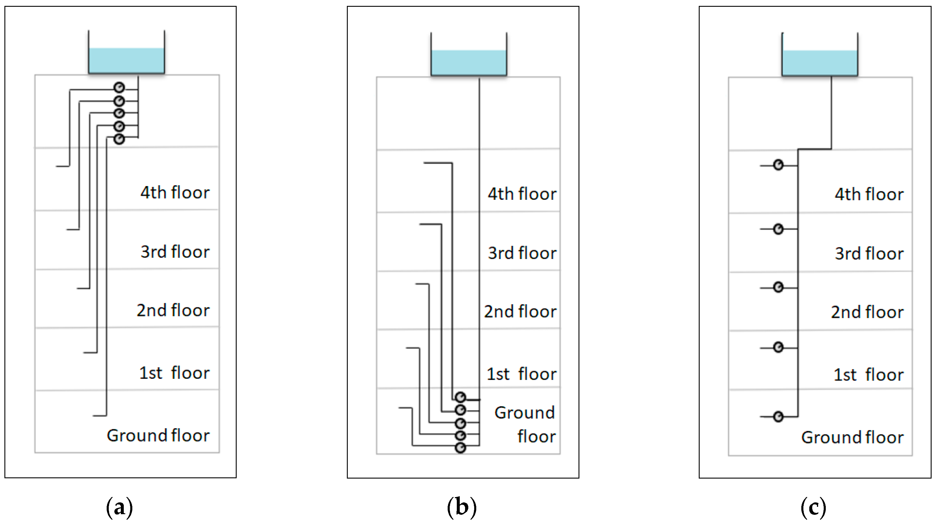
Commonly, the measurement of both collective and individual water consumption is conducted with conventional hydrometers, but their installation for individualization requires adaptation work in most multifamily buildings. In order for the measurement to be individualized, it is necessary to install water meters in each branch of the existing columns (Figure 1a,b). Alternatively, it is necessary to have a place in the common area of the corridors to position the meters and the installation of specific columns with individualized water meters for each autonomous unit (Figure 1c). Noting that in the case of buildings with many floors, the renovation to be carried out is large-scale and very expensive.
Thus, the availability of a flow and/or volume meter that could be more easily integrated into existing hydraulic installations would contribute greatly to the greater dissemination of the individual measurement systems (IMSs) in buildings with collective metering given that individualized measurement provides numerous benefits, both for the owner and for the condominium, as well as for the development of a sustainable society, as it helps in saving water, reduces waste, and financially promotes a reduction in the bill, as pointed out by some case studies identified in the literature [13,14,15]. For example, the study carried out by Souza and Kalbusch, 2017 [14] presents a 34% reduction in per capita consumption of buildings that changes collective measurement to individual measurement.
In this sense, the present research sought to propose and evaluate a new type of hydrometer to promote advances in the study of these water consumption meters, more specifically for measuring the volume of water consumed in autonomous units of residential buildings.
Thereby, this article aims to research and develop a new methodology for measuring water consumption using a thin-film resistive sensor. In addition, the proposal is to use valves (gate valves) commonly present in residential hydraulic systems, consequently dispensing the need for large-scale work to transform the collective measurement of water consumption into individual measurement in autonomous unit buildings; that is, there will be savings in the installation time of individual meters and a faster return on investment due to the installation of the proposed water meters being on a small scale compared to conventional water meters.
Structurally, this work is organized as follows: Section 2 describes the thin-film resistive sensor, the proposed hydrometer, and the setup used in the electromechanical and electrothermal characterizations; the project made in the Ansys® (2021R2) software of the proposed volumetric meter using the bend sensor; the computer simulation via Ansys® software to obtain the relationship between the resistance of the sensor and the water flow in a building pipe; and, still, the electronic circuit simulation via LTSpice XVII® (v. 17.0.30.0) software to obtain a signal with adequate levels and a good signal-to-noise ratio, that is, a less noisy signal. In addition, the theoretical foundations of artificial neural networks are also shown. Section 3 and Section 4 present the results obtained and the discussions and recommendations for future work, respectively.
2. Materials and Methods
2.1. Thin-Film Resistive Sensor
The thin-film resistive sensor used in this work, herein called ‘bend sensor’, is a flexible sensor that varies its electrical resistance, as it is bent. This happens because the sensor is made by combining a single thin layer of a plastic substrate with a resistive material. This type of sensor separates this resistive material into several microcracks when it is bent, which, as a consequence of the bending movement, defines an increase or a decrease in the material’s electrical conductivity [16], and the radius of curvature or sensor angular deflection establishes the sensor electrical resistance.
It is worth mentioning that the bend sensor’s basic electrical characteristics are established according to the resistive material, the substrate, and the type of coating used in its construction. With respect to the resistive material, typically carbon or polymer elements are used. The substrate properties, together with the conductive component, define sensor flexibility. Finally, as for the coating, the bend sensor may not have any type but also might include some type of coating, for example, silicone rubber, adhesive rubber, polyester, or polyimide. It is important to highlight that the coating provides chemical and mechanical protection to the sensor [17].
Because the bend sensor has relevant electromechanical properties, the interest of several researchers is growing. In this way, its application is spread in several areas. Most of the studies related to the bend sensor are in the health sector, in which this type of sensor is used for numerous purposes [18,19,20,21,22,23,24]. In addition, the thin-film resistive sensor is used for other functionalities, such as soil monitoring [25,26]. In turn, unlike these other areas, the water sector does not present many studies using the bend sensor for flow measurement. However, some studies demonstrate the feasibility and applicability of this type of sensor for this purpose. For example, Fan et al. [27] employ the sensor to monitor the airflow velocity in real-time, helping to save energy consumption in a wastewater treatment process; Xu et al. [28] report a way to monitor water flow in pipelines using a flexible resistive film; Srinivasan et al. [29] use the sensor as a cantilever beam to measure the flow for moderate flow applications; and Stewart et al. [30] developed a velocity sensor using the bend sensor for application in streams.
In summary, these thin-film resistive sensors have various applications in the most diverse areas, such as medical, aeronautical, automotive, robotics, and even soil studies. Over the last few years, this type of sensor has attracted a lot of attention from researchers because it can vary its resistance when flexed, as well as being light, robust, and low cost. These sensors are easily adaptable in hydraulic systems of autonomous units (residential, commercial, or mixed) in buildings. In addition, it is possible to design and build interfaces that result in the effective coupling of electronic components with the bend sensor.
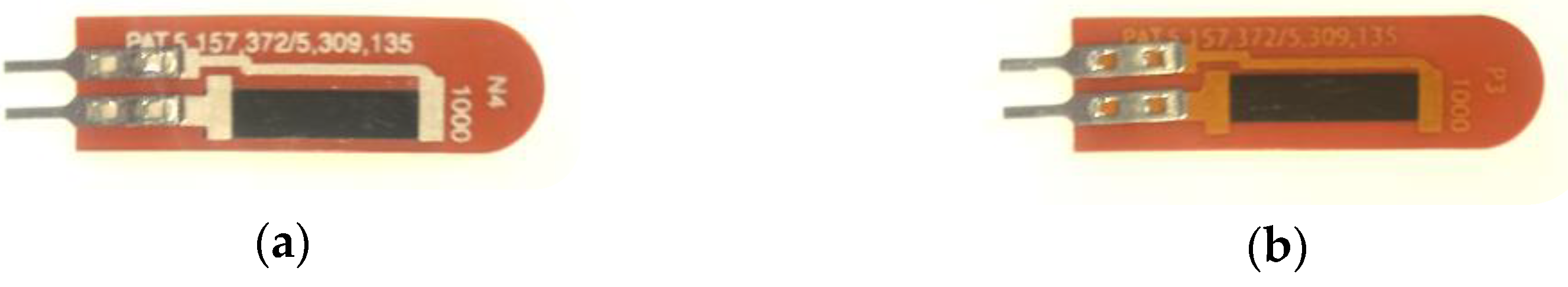
For the development of this study, we used two thin-film resistive sensors from the manufacturer Flexpoint (Figure 2), each one is 1 inch (24.5 mm) long, 0.28 inches (7.11 mm) wide, and 0.005 inches (0.127 mm) thick. Of these two sensors, one is coated with polyester and the other with polyimide.
The new hydrometer proposal—based on a thin-film resistive sensor for measuring water consumption in autonomous units—consists mainly of using flow control valves that are already present in the building’s hydraulic installation.
Thereby, the proposal is to insert the bend sensor into the valve so that it can be adapted to work as a volumetric meter using the valve’s mechanical structure, especially the wedge—the component responsible for the release (valve open) and blockage (valve closed) of the fluid passage. This adaptation is possible because it is feasible to remove the core from these flow control valve types, enabling the use of these valves that are already installed in the piping of buildings.
Figure 3 shows a gate-type flow control valve: In Figure 3a, the valve is open (retracted wedge) with the sensor positioned inside it, allowing the passage and flow measurement, and in Figure 3b, the valve is closed (wedge obstructing the passage), preventing flow.
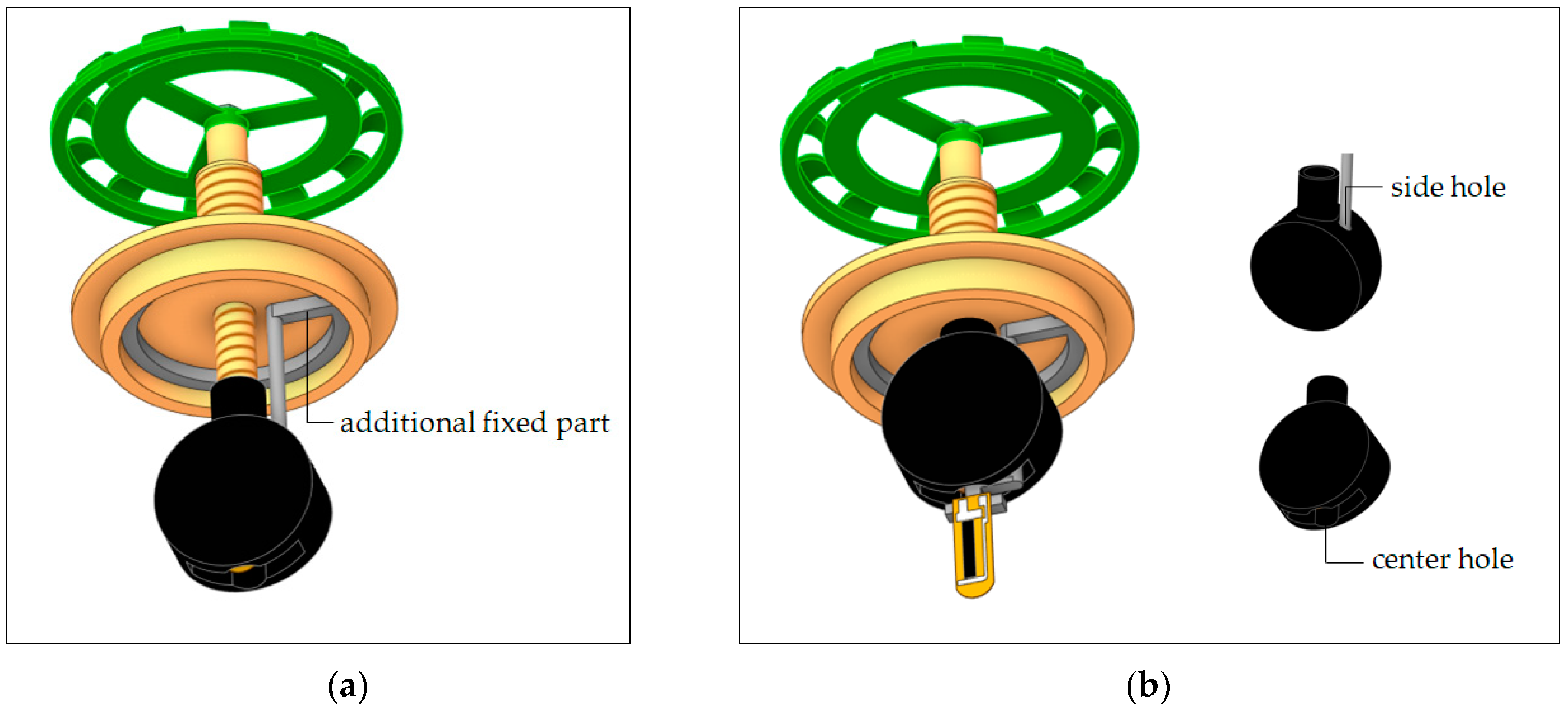
To adapt the valve as a volumetric meter, it is proposed to insert an additional fixed part (gray part) inside the cover (Figure 4a) to work as a support for the bend sensor to be positioned inside the valve. In a meter initial proposal and laboratory evaluation, it is suggested to use epoxy resin for fixing the sensor in this additional part, as this type of resin is highly resistant and even hardens in water, as was performed in the study by Xu et al. [28]. However, due to the epoxy resin toxicity, it is necessary to investigate other material options to be used to fix the sensor within the proposed volumetric meter idea. Furthermore, in practical terms, to standardize the proposed gauge model, it would be necessary to manufacture a wedge with a hole on the side for the gray part to pass through and an opening in the center to make space for the sensor, as shown Figure 4b.
Initially, it was necessary to better understand some properties of the bend sensor and its behavior when flexed at different angles within an exploratory study, which sought to determine the feasibility of using it to measure water consumption. Thus, two types of characterizations of thin-film resistive sensors through different methods were made. The first characterization method sought to evaluate the sensor’s electromechanical behavior, and the second analyzed its electrothermal characteristics.
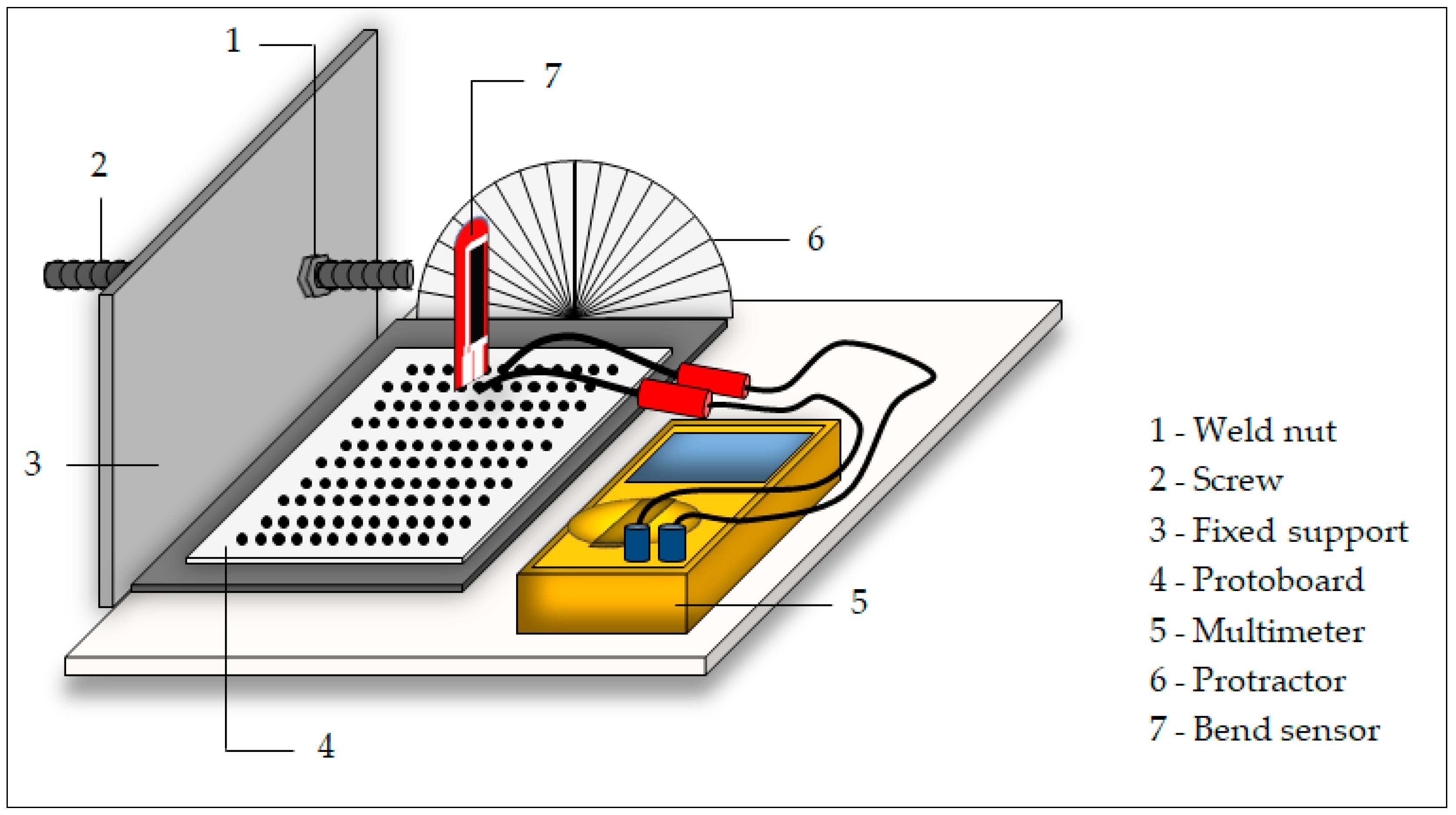
For this, a setup was developed and used in both characterizations, containing a Flexpoint bend sensor, a Keysight U1233A portable digital multimeter, a screw to flex the bend sensor, a fixed support with a welded nut to guide the screw, a protoboard as a base for the bend sensor, and a protractor to measure the sensor bending angle. This setup is shown in Figure 5. Additionally, the same characterizations—electromechanical and thermal—of article [31] were made but with smaller sensors (1 inch). It should be mentioned that this configuration requires the operator to manually flex the bend sensor to the required angle and visually position it. As a result, these measurements are susceptible to parallax errors, so differences in the values measured in the two characterizations may occur.
2.2. Ansys Simulation
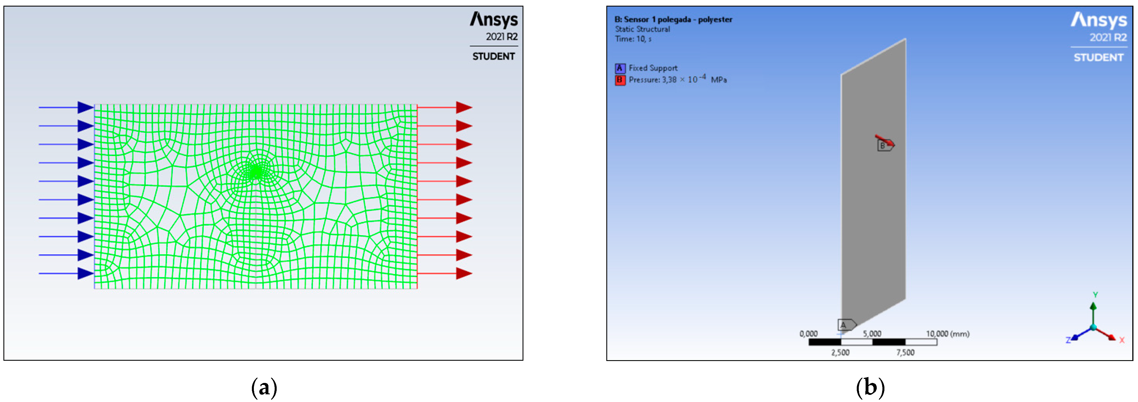
To computationally analyze the sensor bend flexing caused by the flow of water in a pipe, it was necessary to carry out a study through a simulation using computer-aided engineering (CAE) via Ansys® software through a decoupled system. In other words, first, a simulation was carried out in Fluent Ansys® of the water flow inside a pipe to obtain the pressure value (Figure 6a) and, after that, another simulation was carried out in Mechanical Ansys® to obtain the maximum sensor deformation when the pressure calculated in the previous step is applied (Figure 6b).
Methodologically, to simulate the water flow through a pipe, a numerical simulation of computational fluid dynamics (CFD) was performed. The geometry and mesh generation were completed in SpaceClaim, the flow parameters configuration and the numerical solutions were performed in Fluent, and the visualization and analysis were conducted in CFD-Post.
With the aim to configure the simulation of water flow, the Reynolds number (Re) was used according to Equation (1), which is used to determine the flow regime of a given fluid. This regime can be classified as laminar or turbulent depending on the Reynolds number (Re). Typically, in internal flows, Re values lower than 2300 are considered laminar flows, and values higher than 2300 are considered turbulent flows.
where ρ and μ are the fluid and dynamic viscosity, respectively, is the average fluid velocity, and Dh is the hydraulic diameter defined by
where and are, respectively, the cross-sectional area and the wetted perimeter in which the flow occurs.
The velocities used for the flow simulation came from historical data obtained from measurements performed with an ultrasonic flow meter and a 1 ½ inch diameter pipe (typically used in hydraulic systems of autonomous units in residential buildings). These velocities vary between 0.0502 m/s and 0.5307 m/s. Table 1 presents the data used in the one-inch-long resistive sensor simulation and data for calculating the Reynolds number. The fluid used in the simulation was water (μ = 1.003 × 10⁻³ Pa·s and ρ = 998.2 kg/m3 at 20 °C) without considering the air that is commonly present in the pipes.
To generate the velocity field and obtain the pressure value, it was necessary to choose the appropriate flow model for the simulation. For all velocities, the Reynolds number was higher than 2300, thus configuring a turbulent flow, so the turbulence model used was the shear stress transport.
Regarding the simulation via Mechanical Ansys®, the sensor was considered analogous to a cantilever beam subjected to a uniformly distributed load q in which the maximum deflection and the maximum rotation angle occur at the free end of the beam.
Therefore, for the purpose of this study, the method used was finite element analysis. The geometry generation and the sensor parameters configuration, as well as its dimensions and the type of coating (polyester with a density equal to 1380 kg/m3, modulus of elasticity equal to 3.65 GPa, and Poisson’s ratio equal to 0.48 [32]), were performed by the Ansys Workbench.
On the other hand, to configure the structural simulation, the pressure applied to the sensor was obtained with the flow simulation. With this, it was possible to know the maximum deformation corresponding to each speed and, consequently, the sensor’s maximum deflection angle.
Finally, after obtaining these results and using the regression equation obtained in the electromechanical characterization (resistance as a function of deflection angle), it was possible to estimate the resistances for each angle from the simulation (RS).
2.3. LTSpice Simulation
Subsequently, to compose and evaluate the functioning of the proposed water meter, a computer simulation was carried out in LTSpice® of an electronic circuit responsible for powering and conditioning the electrical signals, generating an output voltage related to the flow in the gate valve.
Aiming to perform a simple conversion of deflection to voltage, the bend sensor was connected to a resistor in a voltage divider configuration. The simplest configuration uses just two resistors in series (R1 e R2) and an input voltage (Vin), thus generating an output voltage (Vout) given by
In general, for the purpose of the given electrical voltage signal to have adequate levels and a good signal-to-noise ratio, in other words, the lesser effect of background noise on the signal measurement, it must go through some processes, such as amplification, filtering, and linearization.
The resistance values (RS = R2) obtained from the simulation performed in the Ansys® software were used to properly configure the bend sensor circuit. In addition, using the Solver function of the Excel® (2007) software, another exponential regression (Equation (4)) was performed to obtain a relationship between the simulation resistance (RS) and the flow, which was calculated by multiplying the flow velocity and the pipe cross-section area.
where R0 is the initial resistance, is the instantaneous flow corresponding to the sensor deflection, and is the initial volumetric flow rate.
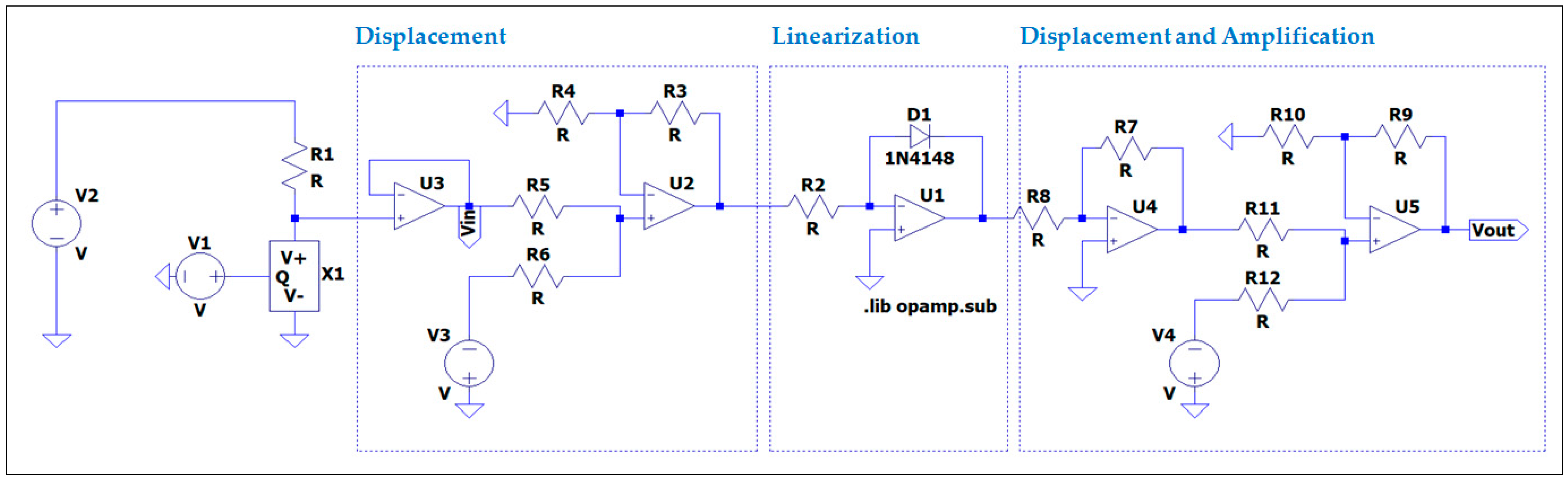
In the simulation in LTSpice®, aiming to obtain a voltage signal as a flow function, a component was created that simulates the bend sensor’s resistive behavior. This component was used in the electronic circuit with processes such as offset, linearization, and amplification. Figure 7 shows how the electronic circuit simulation was performed in this work: (i) The component that simulates the bend sensor (X1) composes a voltage divider with R1, thus generating an output voltage signal (in addition, the resistance value R1 from Figure 7 was chosen to maximize the desired deflection sensitivity range), and (ii) after that, this signal went through the offset, amplification, and linearization processes. Thus, the simulation generated an electrical voltage signal as a flow function with adequate levels and a good signal-to-noise ratio, in other words, with a reduced effect of background noise on the signal measurement.
In this way, the complete system provided a circuit output voltage (output variable Vout) which corresponds to a certain instantaneous flow (input variable controlled by voltage source V1 in Figure 7).
However, for this research, it is necessary to estimate the flow corresponding to this electrical voltage, that is, to obtain the relationship between flow and electrical voltage. For this purpose, the computational intelligence tools called artificial neural networks (ANNs) were used.
2.4. Inverse Problem Solution
In 1943, the first concepts about artificial neural networks were introduced by Warren S. Mcculloch and Walter Pitts [33] who proposed a model of artificial intelligence analogous to the form, behavior, and functions of a biological neuron. In other words, the input signals and the weights from the artificial neuron correspond, respectively, to the dendrites and the synapses—which are the connection of a dendrite with the cell body—from the biological neuron. Furthermore, the stimuli processing is equivalent to the soma function that occurs in the cell body and the activation function and represents the triggering threshold of the biological neuron [34].
Basically, it is enough to combine numerous artificial neurons to obtain the so-called artificial neural networks (ANNs). One of their most relevant purposes is the relationship between independent (input) and dependent (output) variables, which is determined using a learning process in which a set of data is provided to the network. Also noteworthy is the fact that an ANN is a model that does not need to be guided by physical laws; in other words, its parameters do not need to have any physical meaning [35].
Additionally, ANNs have reduced computational time, high precision, and the ability to generate nonlinear relationships between the independent and dependent system variables. Thus, in addition to performing the approximation of functions, ANNs are capable of performing pattern recognition, predictions, and image processing, enabling their application in numerous areas [35], for example, in solar energy systems [36,37,38,39]. ANNs are also used for classification and facial recognition [40,41,42] to create models to predict the condition of airport pavements [43] and for stock market studies [44,45,46,47].
ANNs are also present in research related to water systems, such as in the detection and recognition of leaks in pipes [48,49]; the assessment of the water quality index in the Red Sea, Sudan [50] and the Godavari River, India [51]; and in predicting the efficiency of heavy metal removal from aqueous solutions of biochar systems [52].
In short, these multiple applications are consequences of the artificial neural networks’ various configuration possibilities that can be characterized by the pattern of connections between the units (structure), the learning method, and the activation function [53].
Regarding structure, ANNs can be classified as single-layer or multilayer feedforward networks and recurrent networks. Feedforward networks differ from recurrent networks because they do not have a recurrent loop.
In relation to the learning method, the training model is established by how the parameters are modified, being able to be supervised, unsupervised, and by reinforcement. In supervised mode, the input and output data set are known, but the environment is not known; in other words, the network parameters adjustment is performed by associating the input signal with an error signal (difference between the output signal desired and the one provided by the network). In contrast, the unsupervised one does not require the desired output value from the network—the system collects properties from the patterns set, grouping them into classes inherent to the data. In contrast, the reinforcement training system learns to perform a certain task only based on the results of its experience with an interaction with the environment [54]. Furthermore, it is possible to validate the training model using several algorithms, for example, cross-validation, which is a standard statistical tool that uses a different data set from those used to adjust the network parameters; in other words, the data set is randomly divided into two sets: training—which is subdivided into estimation (used to select the model) and validation (used to test or validate the model)—and test [34].
As for the activation function, it can be from several types, the most used being binary step function, linear function, sigmoid, tanh, ReLU, and radial basis function (RBF).
Thus, in this research, we chose to use a feedforward network with supervised learning and the radial basis function as the activation function (two layers) because other adjustments were tested (for example, exponential and polynomial) but had large errors.
In light of what was presented previously about LTSpice® and ANNs, the following describes what is conventionally called ‘Inverse Problem Solution’: The simulated system generated a voltage signal from the bend sensor as an output having a flow signal as an input; however, for this study, the flow must be the output variable. Therefore, the ANN was used to obtain the volumetric flow rate signal (output) as a voltage function (input). This training was carried out through Matlab’s (R2019b) ‘newrbe’; function—in which the input parameters were the electrical voltages simulated by the LTSpice®, and the outputs were the desired flow rates. With this, it was possible to obtain a trained network that, when receiving the voltage values, estimates the volumetric flow rate values.
Finally, a volume estimate was made by different means—analytical and numerical calculation—aiming at a simulated validation of the proposed measurement concept with the thin-film resistive sensor.
2.5. Simulation of Meter Operation
Assuming that the hydrometer must measure the total volume of water consumed by an autonomous unit, it is understood that the meter proposed in this work needs to estimate the volume from the instantaneous flow.
Because of this, it is necessary to consider the reality of residential building pipes given that water only flows at certain moments, such as when opening a faucet, for example. Therefore, to validate the simulations performed on the proposed hydrometer based on a resistive sensor, two different cases of trapezoidal flow pulses were generated starting from zero (no water flow in the pipe) and reaching a certain flow value, which depends on which hydraulic system was activated.
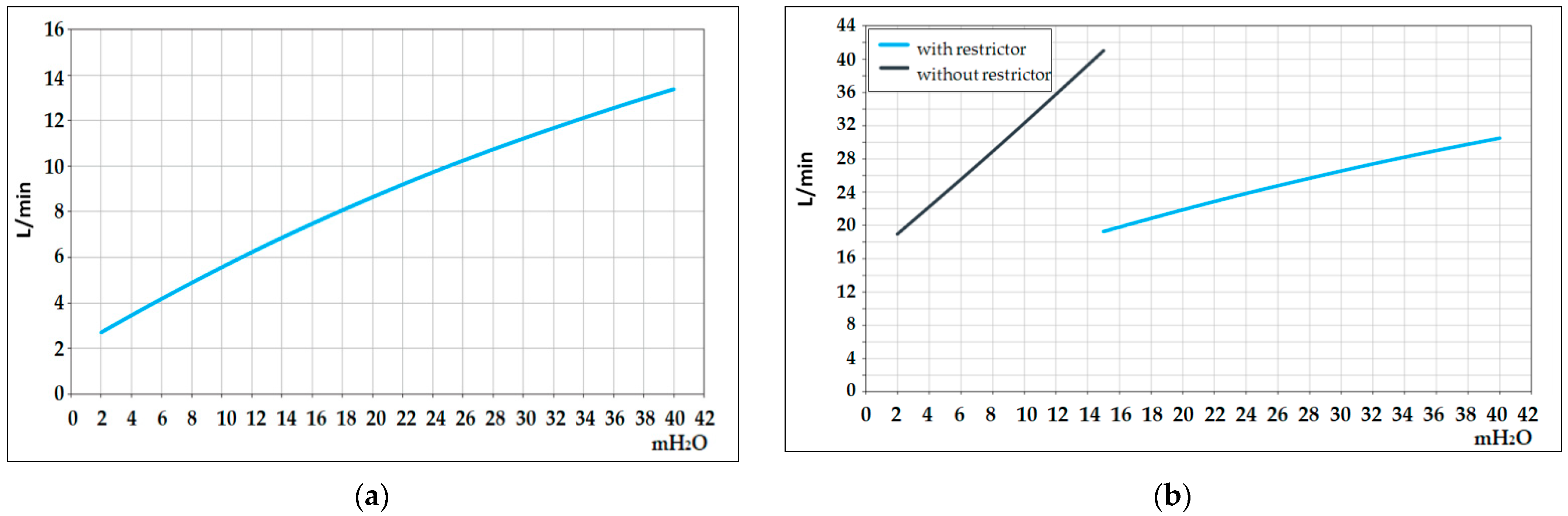
In this research, a water tap—flow curve from the faucet (Figure 8a)—and a conventional shower—flow curve traditional shower (Figure 8b)—both from the manufacturer Docol, were considered to extract the flow values to generate the trapezoidal pulse. To approach a more realistic scenario, small fluctuations in the trapezoidal pulse maximum flow were added, and 15 s faucet activation and 15 min shower using the conventional shower were considered.
The configuration of the trapezoidal pulse in the two cases applied considered a twelve-floor building, and two autonomous units, one on the fourth floor and another on the eleventh floor. It is worth mentioning that, as each floor is 3 m high, the unit on the fourth floor has 24 m of water column (mH2O), and the one on the eleventh has 3 mH2O.
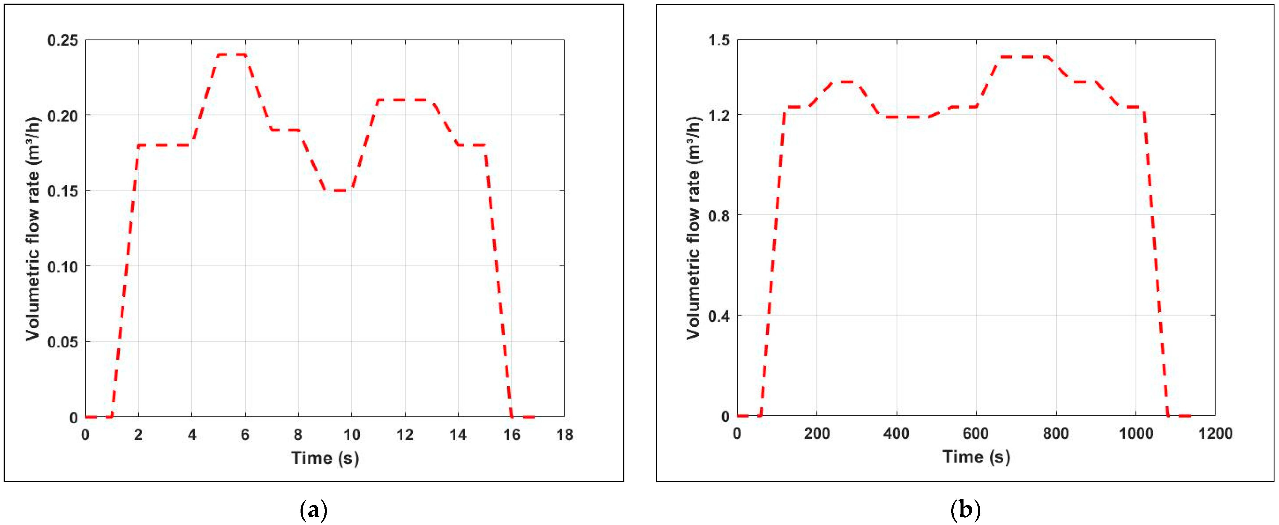
For the fourth floor unit, the faucet has a flow of 9.5 L/min (0.57 m3/h), so the trapezoidal pulse was generated with fluctuations around this flow (Figure 9a), and for the shower—considering the use of a pressure restrictor as indicated by the manufacturer—the pulse was generated around the flow of 24 L/min (1.44 m3/h), as shown in Figure 9b.
Regarding the eleventh floor unit, the faucet trapezoidal pulse is shown in Figure 10a and has fluctuations around the flow rate of 3 L/min (0.18 m3/h). Whereas, for the same unit, the traditional shower without restrictor trapezoidal pulse is shown in Figure 10b and varies around the flow rate of 20.5 L/min (1.23 m3/h).
Subsequently, these pulses were used in the LTSpice® software (defining the values of voltage source V1 in Figure 7) to obtain the sensor output voltage signal. With this, the simulation response of the bend sensor (voltage) towards the hydraulic system activation (flow) was obtained as a function of time. These voltage values were provided to the trained artificial neural network to obtain the corresponding volumetric flow rate output values.
Finally, to estimate the volume from these volumetric flow rates found, two calculations were performed by different means, the first by analytical calculations and the second by numerical calculations.
The analytical estimate was made from the trapezoidal pulse generated using
where is the volumetric flow that represents the volume () of a fluid that flows through a section of a pipe in a time interval ().
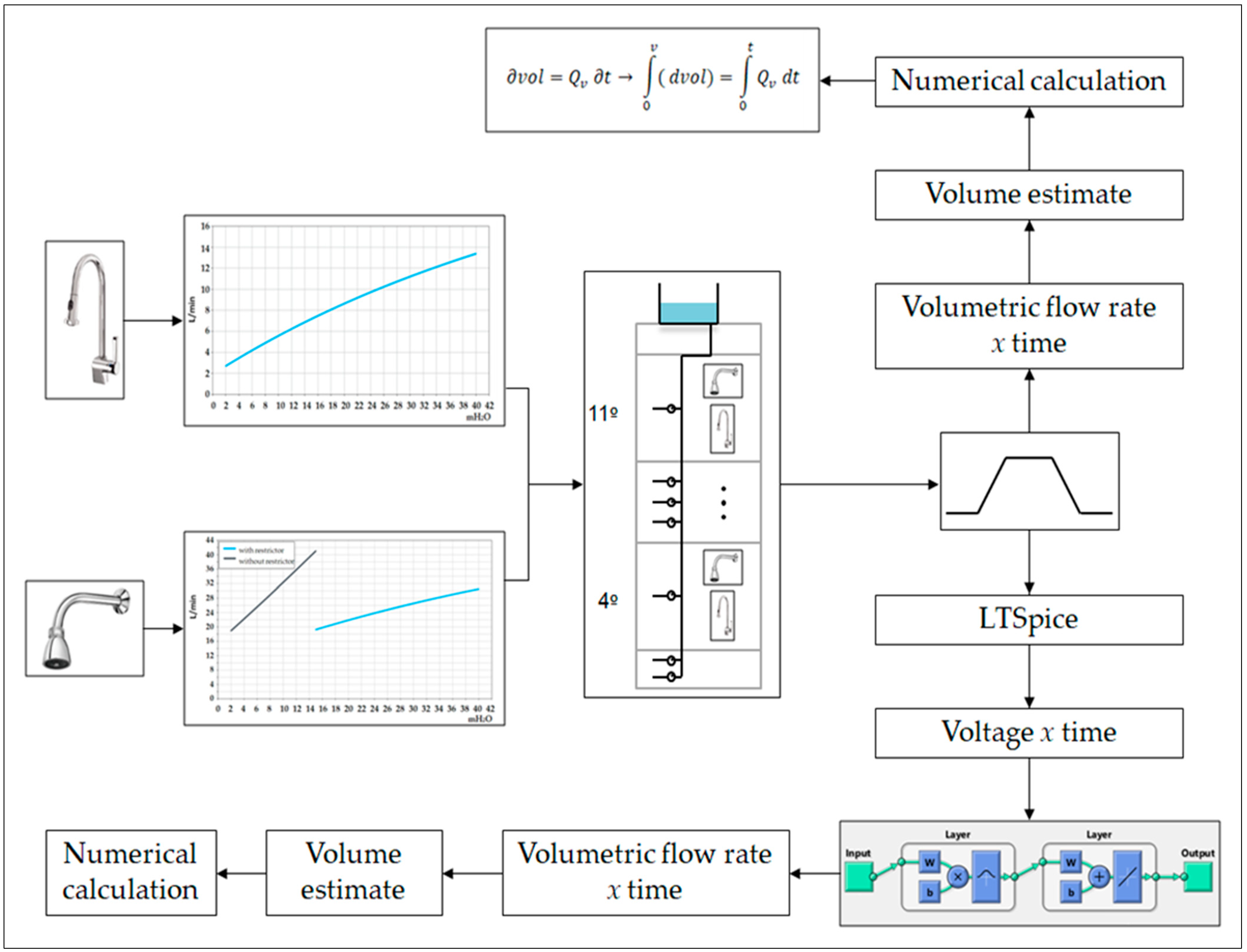
The second estimate, in turn, was performed by numerically integrating the flow values from the neural network using the Matlab software trapezoidal method, resulting in the volume calculation. Figure 11 presents, in a summarized and schematic way, the steps that were performed to obtain the volume by the two methods.
It is important to point out that the pressure value from the hydraulic system flow curve is different from the one from the computer simulation via Fluent Ansys. The first pressure is called static, which corresponds to the pressure of the water when it is stopped in the pipe, and, according to the ABNT NBR 5626 standard, in a building installation, a pressure of 40 mH2O must not be exceeded [55]. On the other hand, the pressure of the computer simulation is called dynamic, which is when there is the movement of water in the pipe at the moment when some hydraulic system is activated. Moreover, dynamic pressure is static pressure minus distributed and localized head losses.
3. Results
This section presents the resistance behavior of thin film resistive sensors when subjected to angular (electromechanical characterization) and temperature (electrothermal characterization) variations; simulations in Ansys and LTSpice® software to find a correlation between the sensor resistance and the flow velocity; and finally, a mathematical formulation for estimating the volume, aiming at the bend sensor application to measure the volume of water drained in a pipe of autonomous units.
Initially, intending to facilitate the understanding of the organization of the content of the results, Figure 12 shows a section mapping.
3.1. Bend Sensor Behavior Evaluation
3.1.1. Electromechanical Characterization
This characterization had, as its principal objective, to know preliminarily the characteristics of the sensor resistance variation in relation to its angular deflection and, consequently, to analyze its behavior. As previously mentioned, two one-inch-long bend sensors with different coatings—one coated with polyester and the other with polyimide-coated—were analyzed.
As this characterization method made it possible to measure the resistances in the increment and decrement of the angle, it was possible to obtain the hysteresis curve and calculate the maximum hysteresis for each sensor bend. The regression equations and the coefficients of determination (R2) were obtained via Excel® software from the average resistances (between the values in the increment and decrement of the angle).
The results for the sensor with polyester coating are shown in Figure 13a. This sensor presented a maximum hysteresis equal to 3.5% of full scale, an average resistance variation between 1.40 kΩ and 5.28 kΩ, and the equation as an exponential regression with a coefficient of determination (R2) of 0.9988. Figure 13b shows the results of the 1-inch-long sensor with a polyimide coating. This sensor showed a maximum hysteresis equal to 13% of the full scale and an average resistance variation between 3.51 kΩ and 10.65 kΩ, and the equation as an exponential regression with the coefficient of determination (R2) of 0.9964.
When considering the change in velocity of the water flow inside a pipe, it becomes imperative that the proposed hydrometer based on a resistive sensor has the lowest possible hysteresis value, in other words, the highest agreement between the ‘loading’ and ‘unloading’ curves. Therefore, comparing these results from the electromechanical characterization, the sensor coated with polyester showed better applicability for measuring water consumption due to having a lower hysteresis value.
On the other hand, given that the proposal is to use the resistive sensor in a pipe to measure the volume of water, this sensor, in turn, must have characteristics that support this type of application. Therefore, the sensors were subjected to electrothermal characterization.
3.1.2. Electrothermal Characterization
The main objective of this characterization was to know and analyze the sensor resistance variation characteristics when subjected to temperature changes. In the same way as the electromechanical characterization, two one-inch-long thin film resistive sensors were evaluated: one with a polyester coating and the other with a polyimide coating. The sensors characterized were the same for both characterizations.
In this methodology, the curvature angle was fixed, and the sensor resistances were measured in the temperature increment and decrement. Consequently, it was feasible to calculate and evaluate the hysteresis concerning the temperature.
First, the polyester-coated bend sensor was characterized. This sensor showed the same behavior for all angles tested when subjected to climatic chamber heating and cooling. As the temperature increased, the sensor resistance decreased, and when the temperature reduced, the resistance increased (Figure 14), noting, thus, a good agreement between the ‘loading’ and ‘unloading’ curves of the sensor.
In the sequence, the other bend sensor characterized was polyimide coated. This sensor, when submitted to the climatic chamber cycle, presented an irregular behavior between the tested angles (Figure 15). At a 0° angle, when heating, the resistance values decreased, and during cooling, these values also decreased (Figure 15a). In turn, for angles of 10°, 30°, 50°, and 60°, this behavior did not remain. At these angles, as the temperature increased, the sensor resistance also increased, and during cooling, as the temperature reduced, the sensor resistance continued to rise (Figure 15b)—thus denoting an irregular behavior between the sensor ‘loading’ and ‘unloading’ curves.
In light of this result, the same characterization was repeated with an identical sensor, having obtained the same results as the first, thus confirming the anomalous behavior of that type of sensor when subjected to the same evaluation conditions.
Thus, the bend sensor with polyester coating showed a more regular and satisfactory behavior demonstrated by a better agreement between the ‘loading’ and ‘unloading’ curves when compared to the sensor with polyimide coating. For this reason, the results obtained from this sensor were plotted, indicating the quantities measured in different ways: from the three-dimensional point of view (Figure 16a) and the bend sensor resistance responses concerning the angle for each temperature (Figure 16b).
In general, when analyzing the results presented, the bend sensor coated with polyester showed a negative linear relationship between the sensor resistance and the temperature variation; in other words, the resistance decreases when the temperature increases.
As this sensor has demonstrated a more stable behavior compared to that of polyimide, as well as a lower hysteresis value in the electrothermal characterization, in terms of applicability, it shows up as being more viable for measuring water consumption in pipes of autonomous units of buildings. For these reasons, only the polyester-coated sensor was used in the Ansys and LTspice® software simulations that follow.
3.2. Computational Simulation
3.2.1. Ansys Simulation
The sensor behavior study was carried out through a computer simulation in Ansys software to evaluate the applicability of the bend sensor for measuring water consumption in autonomous units. The aim was to obtain computationally the sensor deflection angle caused by the flow of water in the pipe and then calculate the corresponding resistances using the regression equation found in Section 3.1.1.
Thus, Table 2 presents the results of the interaction of the water flow in the pipeline with the deflection behavior of the resistive sensor with a polyester coating.
The velocity used in the flow simulation to obtain the pressure to bend the 1-inch-long sensor with polyester coating ranged from 0.15 m/s to 0.58 m/s. As a result, this sensor presented a variation of deflection between 5° and 69° and resistances (Rs) between 1.35 kΩ and 9.25 kΩ.
After completing the modeling to obtain the sensor deflection angle curved by the pressure exerted by the fluid flow inside a pipe, an evaluation more focused on the sensor’s operational aspect was started. For this purpose, a simulation of the electronic circuit to be implemented was performed via LTSpice® software.
3.2.2. LTSpice Simulation
As mentioned previously, only the polyester-coated sensor was used. Thus, it is emphasized that the principal purpose of computationally simulating the electronic circuit was to obtain a relationship between the voltage from the bend sensor with the flow of water.
Therefore, considering the sensor to be one-inch-long, Equation (6)—obtained through the Solver function of the Excel® software—presents the estimated parameters to minimize the error sum of squares.
Thus, Figure 17 presents the resistance response obtained in the simulation via Ansys (RS) as a function of the flow and the adjustment curve with a coefficient of determination (R2) of 0.9972.
Given this, the bend sensor circuit was configured with Equation (6), and the generated signal (X1) passed through the voltage divider (first block of Figure 7), which transformed the resistance signal into voltage and maximized the deflection sensitivity range (R1 = 3 kΩ). After that, the signal went through an offset of 0.3145 V (V3), a gain of 16 v/v (1 + R3/R4), and a linearization process (‘linearization’ block in Figure 7). Finally, it again passed an offset (V4) and a gain (1 + R9/R10) of 1.897 V and 1.769 v/v, respectively.
Once the configuration above was generated with the data obtained from the simulation of the circuit and the conditioners, it was possible to obtain a relationship between voltage and flow, as shown in Figure 18.
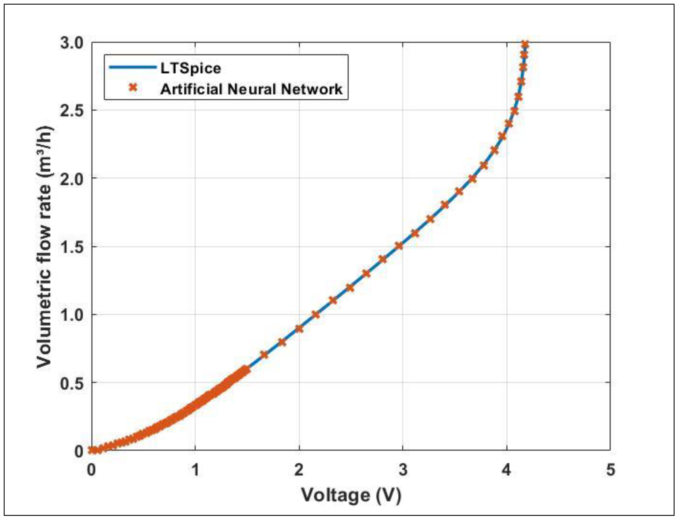
Finally, as previously presented, this relationship between voltage and flow was used to train an artificial neural network that estimated the instantaneous flow values upon receiving the voltage values. The network training results for the one-inch-long sensor are shown in Figure 19.
In this sense, as a hydrometer, conceptually, is an instrument designed for measurement and a continuous indication of the volume of water drained, the meter proposed in this work needs to indicate volume instead of flow. For this reason, in the next step, a volume estimate was performed.
3.3. Meter Operation Simulation
3.3.1. Fourth-Floor Autonomous Unit
The simulation results of the thin-film resistive sensor when the faucet is activated are shown in Figure 20. Figure 20a shows the electrical voltage signal response as a function of the faucet’s operating time. In turn, Figure 20b presents a comparison between the trapezoidal pulse generated by the resistive sensor simulation via an artificial neural network (blue curve) and the faucet flow curve (red dashed curve).
It is worth mentioning that, for the proposed hydrometer, it is necessary to estimate the water volume drained during the 15 s activation of the water tap.
Then, as explained in Section 2.5, the volume was estimated by different means from the flows found. The first method, which was the analytical calculation of the theoretical trapezoidal pulse (faucet flow curve), resulted in a volume of 0.002314 m3 (2.314 L), and the second method, which was the numerical calculation of the trapezoidal pulse obtained via sensor simulation, resulted in 0.002319 m3 (2.319 L) of drained volume.
For the traditional shower activation, the sensor simulation results are shown in Figure 21. In Figure 21a, the electrical voltage signal response is shown as a function of the operating time of the conventional shower. Additionally, Figure 21b presents a comparison between the trapezoidal pulse generated by the resistive sensor simulation via an artificial neural network (blue curve) and the shower flow curve (red dashed curve). By the analytical calculation, the volume of water drained during the traditional shower activation for a 15 min shower was equal to 0.3861 m3 (386.1 L), and by the numerical calculation, it was equal to 0.3858 m3 (385.8 L).
3.3.2. Eleventh-Floor Autonomous Unit
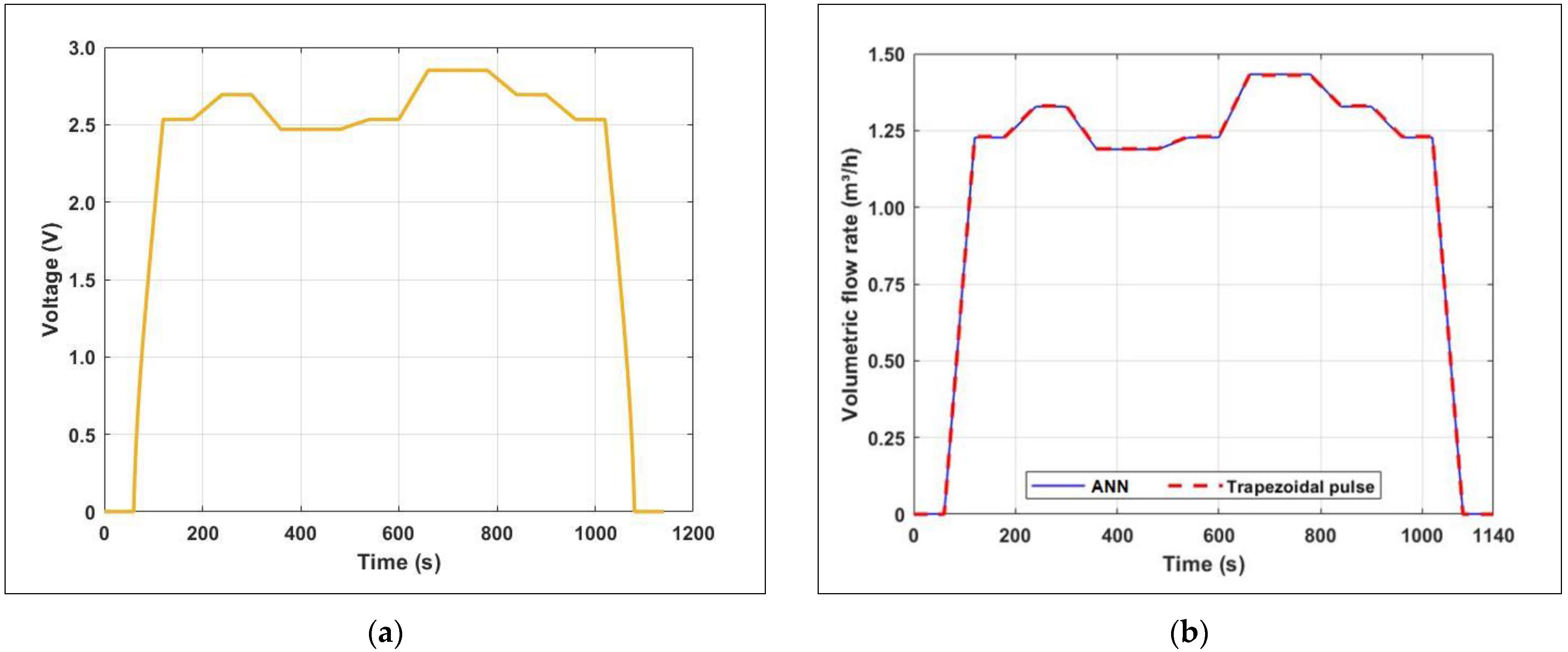
Concerning water tap activation, the sensor simulation results are shown Figure 22. Figure 22a shows the electrical voltage signal response as a function of the faucet operating time. In turn, Figure 22b presents a comparison between the trapezoidal pulse generated by the resistive sensor simulation via an artificial neural network (blue curve) and the faucet flow curve (red dashed curve). By analytical calculation, the volume of water drained during water tap activation for 15 s was equal to 7.472 × 10⁻⁴ m3 (0.07472 L), and by numerical calculation, it was equal to 7.488 × 10⁻⁴ m3 (0.07488 L).
In turn, the sensor simulation results before the traditional shower activation are shown in Figure 23. In Figure 23a, the electrical voltage signal response is shown as a function of the operating time of the shower. Additionally, Figure 23b shows a comparison between the trapezoidal pulse generated by the resistive sensor simulation via an artificial neural network (blue curve) and the shower flow curve (red dashed curve). By the analytical calculation, the volume of water drained during the activation of the shower for a 15 min shower was equal to 0.3427 m3 (342.7 L), and by the numerical calculation, it was equal to 0.3423 m3 (342.3 L).
In summary, Table 3 presents the results described in this section.
These results made it possible to compare the volume calculation in two ways (analytical and numerical). With this, it was possible to perform a simulated validation of the measurement concept.
4. Discussion and Conclusions
From an extensive exploratory study of a thin-film resistive sensor (bend sensor) characterization and simulation, the results reveal the feasibility of the proposed volumetric meter using this type of sensor for volume measurement in autonomous units.
For this, two resistive sensors that were one-inch-long and with different coatings—polyester and polyimide—were electromechanically and thermally characterized. In general, the results obtained from the behavior of the polyimide-coated bend sensor, mainly in the electrothermal characterization, can be considered unexpected because this type of polymer is classified as ultra-performance; in other words, they are super engineering plastics. Polyimide is a material that has significant and particular characteristics, such as high thermal stability, which is one of the main qualities of polyimide, allowing this material to be used for long periods at temperatures up to 200 °C and for a short term at temperatures up to 480 °C without affecting its mechanical behavior [56,57]. Additionally, study [31] corroborates this anomalous behavior of the polyimide-coated bend sensor because in this article, two two-inch-long polyimide-coated sensors were electrothermally characterized and showed the same behavior as the one-inch sensors presented in this article.
Therefore, for the proposed hydrometer, the electrothermal characterization test is more significant, as it is more similar to the reality of residential building pipes. Consequently, because of the results from this characterization, the bend sensor with polyimide coating is unfeasible for measuring the water consumption of autonomous units, as the water meters must be built with materials resistant to temperature variations between +1 °C and +40 °C according to specifications in Brazil by the National Institute of Metrology, Quality, and Technology (INMETRO) [58]. Therefore, considering the intended proposed hydrometer application and the two characterizations, the polyester-coated resistive sensor demonstrated better viability to be used as a transducer.
Concerning the computer simulation, through Ansys, it was fundamental to obtain the relation of the sensor deflection angle, which is curved by the pressure exerted by the fluid flow inside a pipe. The 1-inch-long polyester-coated sensor was simulated using a velocity range between 0.15 m/s and 0.58 m/s. This sensor presented a deflection variation between 5° and 69° and resistance (Rs) between 1.35 kΩ and 9.25 kΩ. These velocities are relevant for piping installation in buildings. In Brazil, for example, the velocity inside the pipe cannot exceed 3 m/s [55].
Regarding the proposed meter operating principle, an electronic circuit simulation was made via LTSpice® software. The simulation resulted in an electrical voltage signal with a larger intensity, a better signal-to-noise ratio, and was as linear as possible as a result of the amplification and linearization processes. In turn, an artificial neural network was trained to obtain the instantaneous volumetric flow rates from the electrical voltage signal. In addition, the results obtained showed promising behavior in the use of these sensors for the desired application.
In addition, a simulated validation of the measurement concept was made considering two autonomous units—one on the fourth floor and another on the eleventh floor—and using two hydraulic systems—a water tap with a 15 s activation and a traditional shower working for 15 min—to validate the simulations performed and estimate the volume from the flow rates of the hydraulic systems. For this, two calculations were performed by different means, the first by analytical calculations and the second by numerical calculations. These results were very similar, which allowed for validation of the simulations performed using Ansys and LTSpice® software and the trained artificial neural network. The 1-inch-long sensor presented a measurement range between 0 m3/h and 3 m3/h (Figure 19). In addition, according to the simulation results, this sensor proved to be capable of measuring the flows of the considered hydraulic systems, in other words, demonstrated to be adequate to work for the application proposed in this research. Furthermore, considering Portaria INMETRO n° 246, from October 17th, 2000 [58], the sensor measurement ranges are relevant for water meters, as this regulation establishes conditions for water volume meters with a nominal flow of 0.6 m3/h at 15.0 m3/h.
Finally, it was possible to define the meter concept by inserting the bend sensor inside the valve so that it can be adapted to work as a volumetric meter. For this, a fixed part was designed inside the valve cover, as shown in Figure 4 (in Section 2), to work as a support for the sensor, and for its fixation in this part, the use of epoxy resin was suggested, as it is highly resistant and hardens even in water, as was performed in the study by Xu et al. [28]. Furthermore, in practical terms, to standardize the proposed meter model, a wedge with a hole on the side for the passage of the support piece and an opening in the center to allow space for the sensor needs to be manufactured, as well as shown in Figure 4b. In addition, still considering the practical aspects, the electrical connection and power source necessary for the proposed hydrometer to work would be solved by a small battery-powered circuit installed next to the valve. For this, some technologies allow for increased battery life, for example, energy harvesting and polling (transmitting data only when new information is available) [59,60,61,62].
In turn, thinking in financial terms and taking into account that the proposed hydrometer will require electronic circuits to measure the voltage, store the readings, and convert them into water consumption, it was possible to estimate the costs of the work to transform the collective measurement water into individual measurements using the hydrometer from this research and a conventional one, as shown in Table 4. These estimates show that the works using the water meter proposed in this article are much cheaper when compared to those using conventional hydrometers.
Therefore, the validation of the thin-film resistive sensor applicability as a transducer of the proposed meter proves to be viable to carry out measurements of the volume of water drained into pipes in autonomous units using flow control valves that are already present in the installation building hydraulics. The proposed water meter complies with Portaria INMETRO n° 246 from 17 October 2000 (Brazilian normative document) [58] under the conditions that the volume meters of cold potable water flowing in a closed pipe must satisfy.
Suggestions for future work to be developed in the continuity of this were proposed:
- The instrumentation of the gate valve through the insertion of the bend sensor inside it, as well as its adaptation as explained through the incorporation of a fixed part and a rubber wedge with a hole on the side and an opening in the center replacing existing wedges;
- To accomplish tests in a hydraulic section to experimentally corroborate the potential of the bend sensor with a polyester coating to measure water consumption in autonomous building units and evaluate the sensor’s long-term behavior (useful life);
- To accomplish additional simulations implementing other scenarios, for example, using flow values lower than those used (leaks), considering air in the pipeline as in reality;
- To realize several bending cycles evaluating the variation in the behavior of the bend sensor, thereby assessing the sensor’s reliability for long-term operation.
Author Contributions
Methodology, L.d.S.G., K.A.R.M. and C.R.H.B.; Software, L.d.S.G., K.A.R.M. and C.R.H.B.; Validation, L.d.S.G., K.A.R.M. and C.R.H.B.; Formal analysis, L.d.S.G., K.A.R.M. and C.R.H.B.; Investigation, L.d.S.G., K.A.R.M. and C.R.H.B.; Resources, K.A.R.M. and C.R.H.B.; Data curation, L.d.S.G. and K.A.R.M.; Writing—original draft, L.d.S.G. and K.A.R.M.; Writing—review & editing, L.d.S.G., K.A.R.M. and C.R.H.B.; Visualization, L.d.S.G.; Supervision, K.A.R.M. and C.R.H.B.; Project administration, K.A.R.M. and C.R.H.B.; Funding acquisition, C.R.H.B.. All authors have read and agreed to the published version of the manuscript.
Funding
This study was financed in part by the Coordenação de Aperfeiçoamento de Pessoal de Nível Superior-Brasil (CAPES)-Finance Code 001.
Data Availability Statement
Not applicable.
Acknowledgments
The authors thank, for the financial support provided, the Brazilian funding agencies CNPq, CAPES, FINEP, and FAPERJ. This study was financed in part by the Coordenação de Aperfeiçoamento de Pessoal de Nível Superior-Brasil (CAPES)-Finance Code 001.
Conflicts of Interest
The authors declare no conflict of interest. In addition, the funders had no role in the design of the study; in the collection, analyses, or interpretation of data; in the writing of the manuscript; or in the decision to publish the results.
References
- Valipour, M.; Krasilnikof, J.; Yannopoulos, S.; Kumar, R.; Deng, J.; Roccaro, P.; Mays, L.; Grismer, M.E.; Angelakis, A.N. The evolution of agricultural drainage from the earliest times to the present. Sustainability 2020, 12, 416. [Google Scholar] [CrossRef] [Green Version]
- Angelakis, A.N.; Zaccaria, D.; Krasilnikoff, J.; Salgot, M.; Bazza, M.; Roccaro, P.; Jimenez, B.; Kumar, A.; Yinghua, W.; Baba, A.; et al. Irrigation of world agricultural lands: Evolution through the millennia. Water 2020, 12, 1285. [Google Scholar] [CrossRef]
- Webster, C. The sewers of Mohenjo-Daro. J. Water Pollut. Control Fed. 1962, 34, 116–123. [Google Scholar]
- De Feo, G.; Angelakis, A.N.; Antoniou, G.P.; El-Gohary, F.; Haut, B.; Passchier, C.W.; Zheng, X.Y. Historical and technical notes on aqueducts from prehistoric to medieval times. Water 2013, 5, 1996–2025. [Google Scholar] [CrossRef] [Green Version]
- Das, M.M.; Das Saikia, M.; Das, B.M. Hydraulics and Hydraulic Machines; PHI Learning: New Delhi, India, 2013. [Google Scholar]
- Fagan, G.G. Bathing in Public in the Roman World; University of Michigan Press: Ann Arbor, MI, USA, 1999. [Google Scholar]
- SNS. Diagnóstico Temático—Serviços de Água e Esgoto: Gestão Técnica de Água—Ano de Referência 2020. 2022. Available online: https://arquivos-snis.mdr.gov.br/DIAGNOSTICO_TEMATICO_GESTAO_TECNICA_DE_AGUA_AE_SNIS_2022.pdf (accessed on 5 September 2022).
- de Moura, M.R.F.; Pereira, I.K.L.; da Silva, S.R.; Baptista, F.M. Measuring individual water consumption: An incentive to urban areas sustainability. Bund. I 2014, 19, 2071–2081. [Google Scholar]
- Ali, A.; Shaikh, I.A.; Abbasi, N.A.; Firdous, N.; Ashraf, M.N. Enhancing water efficiency and wastewater treatment using sustainable technologies: A laboratory and pilot study for adhesive and leather chemicals production. J. Water Process. Eng. 2020, 36, 101308. [Google Scholar] [CrossRef]
- Ozturk, E.; Cinperi, N.C. Water efficiency and wastewater reduction in an integrated woolen textile mill. J. Clean. Prod. 2018, 201, 686–696. [Google Scholar] [CrossRef]
- Gabarda-Mallorquí, A.; Garcia, X.; Ribas, A. Mass tourism and water efficiency in the hotel industry: A case study. Int. J. Hosp. Manag. 2017, 61, 82–93. [Google Scholar] [CrossRef]
- GO Associados. Perdas De Água—Desafios à Disponibilidade Hídrica e Necessidade de Avanço na Eficiência do Saneamento—Ano de Referência 2018. 2020. Available online: https://tratabrasil.org.br/wp-content/uploads/2022/09/Relatorio_Final_-_Estudo_de_Perdas_2020_-_JUNHO_2020.pdf (accessed on 6 November 2021).
- Vesal, M.; Rahmati, M.H.; Hosseinabadi, N.T. The externality from communal metering of residential water: The case of Tehran. Water Resour. Econ. 2018, 23, 53–58. [Google Scholar] [CrossRef]
- De Souza, C.; Kalbusch, A. Estimation of water consumption in multifamily residential buildings. Acta Sci. Technol. 2017, 39, 161–168. [Google Scholar] [CrossRef] [Green Version]
- Castillo-Manzano, J.I.; Lopez-Valpuesta, L.; Marchena-Gómez, M.; Pedregal, D.J. How much does water consumption drop when each household takes charge of its own consumption? The case of the city of Seville. Appl. Econ. 2013, 45, 4465–4473. [Google Scholar] [CrossRef]
- Orengo, G.; Sbernini, L.; Lorenzo, N.D.; Lagati, A.; Saggio, G. Curvature characterization of flex sensors for human posture recognition. Univers. J. Biomed. Eng. 2013, 1, 10–15. [Google Scholar] [CrossRef]
- Saggio, G.; Riillo, F.; Sbernini, L.; Quitadamo, L.R. Resistive flex sensors: A survey. Smart Mater. Struct. 2015, 25, 13001. [Google Scholar] [CrossRef]
- Saggio, G.; Orengo, G. Flex sensor characterization against shape and curvature changes. Sens. Actuators A Phys. 2018, 273, 221–231. [Google Scholar] [CrossRef]
- Saggio, G. A novel array of flex sensors for a goniometric glove. Sens. Actuators A Phys. 2014, 205, 119–125. [Google Scholar] [CrossRef]
- Guo, Y.R.; Zhang, X.C.; An, N. Monitoring neck posture with flex sensors. In Proceedings of the 9th International Conference on Information Science and Technology, Hulunbuir, China, 2–5 August 2019. [Google Scholar] [CrossRef]
- Borges, L.M.; Barroca, N.; Velez, F.J.; Lebres, A.S. Smart-clothing wireless flex sensor Belt network for foetal health monitoring. In Proceedings of the 3rd International Conference on Pervasive Computing Technologies for Healthcare, London, UK, 1–3 April 2009. [Google Scholar] [CrossRef]
- Jabin, J.; Chowdhury, A.M.; Adnan, M.E.; Islam, M.R.; Mahmud, S.S. Low cost 3D printed prosthetic for congenital amputation using flex sensor. In Proceedings of the 5th International Conference on Advances in Electrical Engineering, Dhaka, Bangladesh, 26–28 September 2019. [Google Scholar] [CrossRef]
- Hu, Q.; Tang, X.; Tang, W. A smart chair sitting posture recognition system using flex sensors and FPGA implemented artificial neural network. IEEE Sens. J. 2020, 20, 8007–8016. [Google Scholar] [CrossRef]
- Starck, J.R.; Murray, G.; Lawford, P.V.; Hose, D.R. An inexpensive sensor for measuring surface geometry. Med. Eng. Phys. 1999, 21, 725–729. [Google Scholar] [CrossRef]
- Yao, C.; Hong, C.; Su, D.; Zhang, Y.; Yin, Z. Design and verification of a wireless sensing system for monitoring large-range ground movement. Sens. Actuators A Phys. 2020, 303, 111745. [Google Scholar] [CrossRef]
- Ramesh, M.V.; Vidya, P.T.; Pradeep, P. Context aware wireless sensor system integrated with participatory sensing for real time road accident detection. In Proceedings of the 10th International Conference on Wireless and Optical Communications Networks, Bhopal, India, 26–28 July 2013. [Google Scholar] [CrossRef]
- Fan, Y.; Dai, Z.; Xu, Z.; Zheng, S.; Dehkordy, F.M.; Bagtzoglou, A.; Zhang, W.; Gao, P.; Li, B. High resolution air flow velocity monitoring using air flow resistance-type sensor film (AFRSF). Sens. Actuators A Phys. 2019, 297, 111562. [Google Scholar] [CrossRef]
- Xu, Z.; Fan, Y.; Wang, T.; Huang, Y.; Dehkordy, F.M.; Dai, Z.; Xia, L.; Dong, Q.; Bagtzoglou, A.; McCutcheon, J.; et al. Towards high resolution monitoring of water flow velocity using flat flexible thin mm-sized resistance-typed sensor film (MRSF). Water Res. X 2019, 4, 100028. [Google Scholar] [CrossRef]
- Srinivasan, C.R.; Sen, S.; Kumar, A.; Saibabu, C. Measurement of flow using bend sensor. In Proceedings of the International Conference on Advances in Energy Conversion Technologies, Manipal, India, 23–25 January 2014. [Google Scholar] [CrossRef]
- Stewart, R.L.; Fox, J.F.; Harnett, C.K. Time-average velocity and turbulence measurement using wireless bend sensors in an open channel with a rough bed. J. Hydraul. Eng. 2013, 139, 696–706. [Google Scholar] [CrossRef] [Green Version]
- Gonçalves, L.d.S.; Medeiros, K.A.R.; Barbosa, C.R.H. Proposition of water meter for buildings based on a thin-film resistive sensor: Electromechanical and thermal characterizations. In Proceedings of the 11° Congresso Brasileiro de Metrologia, Rio de Janeiro, Brazil, 18–21 October 2021. [Google Scholar]
- MatWeb. Overview of Materials for Polyester Film. Available online: http://www.matweb.com/search/DataSheet.aspx?MatGUID=40559706b4fd4aa0a43f5739799728f5&ckck=1 (accessed on 2 March 2021).
- Mcculloch, W.S.; Pitts, W. A logical calculus of ideas immanent in nervous activity. Bull. Math. Biophys. 1943, 5, 115–133. [Google Scholar] [CrossRef]
- Haykin, S. Neural Networks: A Comprehensive Foundation; Prentice Hall: Hoboken, NJ, USA, 1999. [Google Scholar]
- Jawad, J.; Hawari, A.H.; Zaidi, S.J. Artificial neural network modeling of wastewater treatment and desalination using membrane processes: A review. Chem. Eng. J. 2021, 419, 129540. [Google Scholar] [CrossRef]
- Taki, M.; Ajabshirchi, Y.; Ranjbar, S.F.; Rohani, A.; Matloobi, M. Heat transfer and MLP neural network models to predict inside environment variables and energy lost in a semi-solar greenhouse. Energy Build. 2016, 110, 314–329. [Google Scholar] [CrossRef]
- Ghritlahre, H.K.; Prasad, R.K. Prediction of thermal performance of unidirectional flow porous bed solar air heater with optimal training function using artificial neural network. Energy Procedia 2017, 109, 369–376. [Google Scholar] [CrossRef]
- Cetiner, C.; Halici, F.; Cacur, H.; Taymaz, I. Generating hot water by solar energy and application of neural network. Appl. Therm. Eng. 2005, 25, 1337–1348. [Google Scholar] [CrossRef]
- Bala, B.K.; Ashraf, M.A.; Uddin, M.A.; Janjai, S. Experimental and neural network prediction of the performance of a solar tunnel drier for drying jackfruit bulbs and leather. J. Food Process. Eng. 2005, 28, 552–566. [Google Scholar] [CrossRef]
- Saxena, N.; Varshney, D. Smart home security solutions using facial authentication and speaker recognition through artificial neural networks. Int. J. Cogn. Comput. Eng. 2021, 2, 154–164. [Google Scholar] [CrossRef]
- Reddy, K.R.L.; Babu, G.R.; Kishore, L. Face Recognition based on eigen features of multi scaled face components and an artificial neural network. Procedia Comput. Sci. 2010, 2, 62–74. [Google Scholar] [CrossRef] [Green Version]
- Kumar, A. Comparative analysis of RBF (Radial Basis Function) network and gaussian function in multi-layer feed-forward neural network (MLFFNN) for the case of face recognition. Int. J. Adv. Res. 2017, 5, 843–873. [Google Scholar] [CrossRef] [Green Version]
- Baldo, N.; Miani, M.; Rondinella, F.; Celauro, C. Artificial neural network prediction of airport pavement moduli using interpolated surface deflection data. IOP Conf. Ser. Mater. Sci. Eng. 2021, 1203, 022112. [Google Scholar] [CrossRef]
- Bisoi, R.; Dash, P.K. A hybrid evolutionary dynamic neural network for stock market trend analysis and prediction using unscented Kalman filter. Appl. Soft Comput. J. 2014, 19, 41–56. [Google Scholar] [CrossRef]
- Hu, H.; Tang, L.; Zhang, S.; Wang, H. Predicting the direction of stock markets using optimized neural networks with Google Trends. Neurocomputing 2018, 285, 188–195. [Google Scholar] [CrossRef]
- Moghar, A.; Hamiche, M. Stock market prediction using LSTM recurrent neural network. Procedia Comput. Sci. 2020, 170, 1168–1173. [Google Scholar] [CrossRef]
- Chhajer, P.; Shah, M.; Kshirsagar, A. The applications of artificial neural networks, support vector machines, and long–short term memory for stock market prediction. Decis. Anal. J. 2022, 2, 100015. [Google Scholar] [CrossRef]
- Wang, W.; Sun, H.; Guo, J.; Lao, L.; Wu, S.; Zhang, J. Experimental study on water pipeline leak using in-pipe acoustic signal analysis and artificial neural network Prediction. Meas. J. Int. Meas. Confed. 2021, 186, 110094. [Google Scholar] [CrossRef]
- Pérez-Pérez, E.J.; López-Estrada, F.R.; Valencia-Palomo, G.; Torres, L.; Puig, V.; Mina-Antonio, J.D. Leak diagnosis in pipelines using a combined artificial neural network approach. Control Eng. Pract. 2021, 107, 104677. [Google Scholar] [CrossRef]
- Ismael, M.; Mokhtar, A.; Farooq, M.; Lü, X. Assessing drinking water quality based on physical, chemical and microbial parameters in the red sea state, Sudan using a combination of water quality index and artificial neural network model. Groundw. Sustain. Dev. 2021, 14, 100612. [Google Scholar] [CrossRef]
- Nayak, J.G.; Patil, L.G.; Patki, V.K. Artificial neural network based water quality index (WQI) for river Godavari (India). Mater. Today Proc. 2021, in press. [CrossRef]
- Zheng, X.; Nguyen, H. A novel artificial intelligent model for predicting water treatment efficiency of various biochar systems based on artificial neural network and queuing search algorithm. Chemosphere 2022, 287, 132251. [Google Scholar] [CrossRef]
- López, O.A.M.; López, A.M.; Crossa, J. Multivariate Statistical Machine Learning Methods for Genomic Prediction; Springer International Publishing: Cham, Switzerland, 2022. [Google Scholar]
- Sutton, R.S.; Barto, A.G. Reinforcement Learning: An Introduction, 2nd ed.; The MIT Press: Cambridge, MA, USA, 2018. [Google Scholar]
- NBR 5626; Instalação Predial de Ágia Fria. Associação Brasileira de Normas Técnicas—ABNT: Rio de Janeiro, Brazil, 1998; Volume 41.
- Sroog, C.E. Polyimides. Prog. Polym. Sci. 1991, 16, 561–694. [Google Scholar] [CrossRef]
- Liaw, D.J.; Wang, K.L.; Huang, Y.C.; Lee, K.R.; Lai, J.Y.; Ha, C.S. Advanced polyimide materials: Syntheses, physical properties and applications. Prog. Polym. Sci. 2012, 37, 907–974. [Google Scholar] [CrossRef]
- Instituto Nacional De Metrologia Normalização E Qualidade—Inmetro. Portaria nº 246 de 17 de outubro de 2000. Diário Of. da República Fed. do Bras. 2000. Available online: http://www.inmetro.gov.br/legislacao/rtac/pdf/rtac000667.pdf (accessed on 2 July 2021).
- Buennemeyer, T.K.; Nelson, T.M.; Gora, M.A.; Marchany, R.C.; Tront, J.G. Battery polling and trace determination for bluetooth attack detection in mobile devices. In Proceedings of the 2007 IEEE Workshop on Information Assurance, New York, NY, USA, 20–22 June 2007. [Google Scholar] [CrossRef] [Green Version]
- Morris, N.M. Interrupts and polling. In Microprocessor and Microcomputer Technology; Palgrave: London, UK, 1981; pp. 173–186. [Google Scholar]
- Mateu, L.; Moll, F. Review of energy harvesting techniques and applications for microelectronics. In Proceedings of the SPIE 5837, VLSI Circuits and Systems II, Sevilla, Spain, 30 June 2005. [Google Scholar] [CrossRef]
- Kim, T.Y.; Kim, S.K.; Kim, S.W. Application of ferroelectric materials for improving output power of energy harvesters. Nano Converg. 2018, 5, 30. [Google Scholar] [CrossRef] [PubMed] [Green Version]
Figure 1.
Possible locations for hydrometers: (a) on the top floor; (b) on the ground floor; and (c) on the building floors.
Figure 1.
Possible locations for hydrometers: (a) on the top floor; (b) on the ground floor; and (c) on the building floors.

Figure 2.
1-inch bend resistive sensors: (a) polyester bend sensor and (b) polyimide bend sensor.

Figure 3.
Gate valve 3D drawing: (a) open and (b) closed.

Figure 4.
Gate valve cover with rubber wedge fitted with the sensor fixed to the gray part: (a) valve closed and (b) valve open.
Figure 4.
Gate valve cover with rubber wedge fitted with the sensor fixed to the gray part: (a) valve closed and (b) valve open.

Figure 5.
Test setup schematic representation.

Figure 6.
Ansys simulation: (a) Fluent Ansys for obtaining the pressure value and (b) Mechanical Ansys for estimating the sensor maximum deformation.
Figure 6.
Ansys simulation: (a) Fluent Ansys for obtaining the pressure value and (b) Mechanical Ansys for estimating the sensor maximum deformation.

Figure 7.
Electronic circuit configuration in LTSpice®.

Figure 8.
Flow curve from the manufacturer Docol: (a) water tap and (b) traditional shower.

Figure 9.
Trapezoidal pulse for 4th floor autonomous unit of the: (a) water tap and (b) traditional shower.
Figure 9.
Trapezoidal pulse for 4th floor autonomous unit of the: (a) water tap and (b) traditional shower.

Figure 10.
Trapezoidal pulse for 11th floor autonomous unit of the: (a) faucet and (b) traditional shower.
Figure 10.
Trapezoidal pulse for 11th floor autonomous unit of the: (a) faucet and (b) traditional shower.

Figure 11.
Schematic representation of the steps taken to validate the measurement concept of the proposed meter.
Figure 11.
Schematic representation of the steps taken to validate the measurement concept of the proposed meter.

Figure 12.
Content mapping of Section 3.
Figure 12.
Content mapping of Section 3.

Figure 13.
Average and adjusted resistance as a function of the bend sensor deflection angle with (a) polyester coating and (b) polyimide coating.
Figure 13.
Average and adjusted resistance as a function of the bend sensor deflection angle with (a) polyester coating and (b) polyimide coating.

Figure 14.
Resistance of the polyester-coated bend sensor to temperature variation for deflection angles: (a) 0° and 10° and (b) 30°, 50°, and 60°.
Figure 14.
Resistance of the polyester-coated bend sensor to temperature variation for deflection angles: (a) 0° and 10° and (b) 30°, 50°, and 60°.

Figure 15.
Resistance of the polyimide-coated bend sensor to temperature variation for deflection angles: (a) 0°, 10°, and 30° and (b) 50° and 60°.
Figure 15.
Resistance of the polyimide-coated bend sensor to temperature variation for deflection angles: (a) 0°, 10°, and 30° and (b) 50° and 60°.

Figure 16.
Response of the polyester-coated bend sensor: (a) the average resistance between the temperature increment and decrement values for each angle through 3D measured quantities graph and (b) the average resistance as a function of angle of deflection.
Figure 16.
Response of the polyester-coated bend sensor: (a) the average resistance between the temperature increment and decrement values for each angle through 3D measured quantities graph and (b) the average resistance as a function of angle of deflection.

Figure 17.
Resistance response as a function of flow via simulation (green) and regression (blue).

Figure 18.
Polyester-coated bend sensor voltage ratio as a function of flow.

Figure 19.
Result of training the network to obtain the instantaneous flow corresponding the voltage of the one-inch-long, polyester-coated bend sensor.
Figure 19.
Result of training the network to obtain the instantaneous flow corresponding the voltage of the one-inch-long, polyester-coated bend sensor.

Figure 20.
(a) Sensor response to faucet activation and (b) trapezoidal pulse via the bend sensor simulation on the ANN (blue curve) and faucet flow curve for the autonomous unit with 24 mH2O (dashed red curve).
Figure 20.
(a) Sensor response to faucet activation and (b) trapezoidal pulse via the bend sensor simulation on the ANN (blue curve) and faucet flow curve for the autonomous unit with 24 mH2O (dashed red curve).

Figure 21.
(a) Sensor response to the activation of the traditional shower and (b) trapezoidal pulse via the bend sensor simulation on the ANN (blue curve) and traditional shower flow curve for the autonomous unit with 24 mH2O (dashed red curve).
Figure 21.
(a) Sensor response to the activation of the traditional shower and (b) trapezoidal pulse via the bend sensor simulation on the ANN (blue curve) and traditional shower flow curve for the autonomous unit with 24 mH2O (dashed red curve).

Figure 22.
(a) Sensor response to faucet activation and (b) trapezoidal pulse via the bend sensor simulation on the ANN (blue curve) and faucet flow curve for the autonomous unit with 3 mH2O (dashed red curve).
Figure 22.
(a) Sensor response to faucet activation and (b) trapezoidal pulse via the bend sensor simulation on the ANN (blue curve) and faucet flow curve for the autonomous unit with 3 mH2O (dashed red curve).

Figure 23.
(a) Sensor response to the activation of the traditional shower and (b) trapezoidal pulse via simulation of the bend sensor on the ANN (blue curve) and traditional shower flow curve for the autonomous unit with 3 mH2O (dashed red curve).
Figure 23.
(a) Sensor response to the activation of the traditional shower and (b) trapezoidal pulse via simulation of the bend sensor on the ANN (blue curve) and traditional shower flow curve for the autonomous unit with 3 mH2O (dashed red curve).


Table 1.
Data used in the CFD simulation of the bend sensor.
| Parameters | Value | Units | ||
|---|---|---|---|---|
| Inner diameter D | 1 ½ | inch | ||
| 0.0381 | m | |||
| Area A | 0.00114 | m | ||
| Wetted perimeter P | 0.1197 | m | ||
| Hydraulic diameter Dh | 0.0381 | m | ||
| Reynolds number | velocity | max. | 21,992 | - |
| min. | 5688 | |||
Table 2.
Ansys® simulation results with the polyester-coated bend sensor.
| v | Re | Pressure | Deformation | Deflection Angle | RS |
|---|---|---|---|---|---|
| (m/s) | (Dimensionless) | (Pa) | (mm) | (°) | (kΩ) |
| 0.58 | 21,992 | 287 | 22.92 | 69 | 9.25 |
| 0.53 | 19,954 | 240 | 19.17 | 58 | 4.64 |
| 0.47 | 17,916 | 189 | 15.09 | 45 | 2.61 |
| 0.42 | 15,878 | 151 | 12.06 | 36 | 1.95 |
| 0.37 | 13,840 | 117 | 9.34 | 28 | 1.65 |
| 0.31 | 11,802 | 81.8 | 6.53 | 20 | 1.49 |
| 0.26 | 9764 | 57.7 | 4.61 | 14 | 1.42 |
| 0.20 | 7726 | 34.1 | 2.72 | 8 | 1.36 |
| 0.15 | 5688 | 19.2 | 1.53 | 5 | 1.35 |
Table 3.
Volume calculation results.
| Floor | Hydraulic Systems | Volume Estimate (L) | |
|---|---|---|---|
| Analytical | Numerical | ||
| 4th | Water tap | 2.314 | 2.319 |
| Traditional shower | 386.1 | 385.8 | |
| 11th | Water tap | 0.07472 | 0.07488 |
| Traditional shower | 342.7 | 342.3 | |
Table 4.
Estimate of the cost of work to the transformation from the collective measurement of water into individual measurement.
Table 4.
Estimate of the cost of work to the transformation from the collective measurement of water into individual measurement.
| The Transformation from the Collective Measurement of Water into Individual Measurement for a Reasonably Large Building | |||
|---|---|---|---|
| With Conventional Hydrometer | With Proposed Hydrometer | ||
| Number of autonomous units | 160 | 160 | 48 |
| Cost of work (USD) | 180,000 | 32,000 | 9600 |
Disclaimer/Publisher’s Note: The statements, opinions and data contained in all publications are solely those of the individual author(s) and contributor(s) and not of MDPI and/or the editor(s). MDPI and/or the editor(s) disclaim responsibility for any injury to people or property resulting from any ideas, methods, instructions or products referred to in the content. |
© 2023 by the authors. Licensee MDPI, Basel, Switzerland. This article is an open access article distributed under the terms and conditions of the Creative Commons Attribution (CC BY) license (https://creativecommons.org/licenses/by/4.0/).
Share and Cite
MDPI and ACS Style
Gonçalves, L.d.S.; Medeiros, K.A.R.; Barbosa, C.R.H. Hydrometer Design Based on Thin-Film Resistive Sensor for Water Measurement in Residential Buildings. Water 2023, 15, 1045. https://doi.org/10.3390/w15061045
AMA Style
Gonçalves LdS, Medeiros KAR, Barbosa CRH. Hydrometer Design Based on Thin-Film Resistive Sensor for Water Measurement in Residential Buildings. Water. 2023; 15(6):1045. https://doi.org/10.3390/w15061045
Chicago/Turabian StyleGonçalves, Laís dos S., Khrissy A. R. Medeiros, and Carlos R. Hall Barbosa. 2023. "Hydrometer Design Based on Thin-Film Resistive Sensor for Water Measurement in Residential Buildings" Water 15, no. 6: 1045. https://doi.org/10.3390/w15061045
Note that from the first issue of 2016, this journal uses article numbers instead of page numbers. See further details here.