Next Article in Journal
Characterization and Disinfection by Product Formation of Dissolved Organic Matter in Anaerobic–Anoxic–Oxic Membrane Bioreactor (AAO-MBR) Process
Next Article in Special Issue
Improvement of Hargreaves–Samani Reference Evapotranspiration Estimates in the Peruvian Altiplano
Previous Article in Journal
Forecasting Monthly Water Deficit Based on Multi-Variable Linear Regression and Random Forest Models
Previous Article in Special Issue
CSM-CERES-Wheat Sensitivity to Evapotranspiration Modeling Frameworks under a Range of Wind Speeds
 
 
water-logo
Article Menu

Article Menu

Article

Estimation of the Evapotranspiration of Irrigated Açaí (Euterpe oleracea M.), through the Surface Energy Balance Algorithm for Land—SEBAL, in Eastern Amazonia

by
Paulo Jorge de Oliveira Ponte de Souza
1,*,
Ewelyn Regina Rocha Silva
1,
Bernardo Barbosa da Silva
2,
Thomás Rocha Ferreira
2,
Denis de Pinho Sousa
1,
Denilson Barreto da Luz
1,
Marcos Adami
3,
Adriano Marlison Leão de Sousa
1,
Hildo Giuseppe Garcia Caldas Nunes
1,
Gabriel Siqueira Tavares Fernandes
1,
João Vitor de Nóvoa Pinto
1,
Vivian Dielly da Silva Farias
4,
Israel Alves de Oliveira
5,
Sandra Andrea Santos da Silva
4,
José Farias Costa
4,
Matheus Lima Rua
1,
Deborah Luciany Pires Costa
1,
Vandeilson Belfort Moura
1,
Marcus José Alves de Lima
1,
Jannaylton Everton Oliveira Santos
1,
Antonio José da Silva Sousa
6 and
Samuel Ortega-Farias
7
add Show full author list remove Hide full author list
1
Grupo de Pesquisa Interações Solo-Planta-Atmosfera na Amazônia, Instituto Socioambiental e dos Recursos Hídricos, Campus Belém, Universidade Federal Rural da Amazônia, Belém 66077-830, PA, Brazil
2
Centro de Tecnologia e Recursos Naturais, Campus Campina Grande, Universidade Federal de Campina Grande, Campina Grande 58429-900, PB, Brazil
3
Divisão de Observação da Terra e Geoinformática, Instituto Nacional de Pesquisas Espaciais, São José dos Campos 12227-010, SP, Brazil
4
Faculdade de Engenharia Agronômica, Campus de Altamira, Universidade Federal do Pará, Altamira 68372-040, PA, Brazil
5
Instituto de Desenvolvimento Florestal e da Biodiversidade do Estado do Pará, Altamira 66087-812, PA, Brazil
6
Secretaria de Estado de Meio Ambiente e Sustentabilidade, Belém 66093-677, PA, Brazil
7
Centro de Investigación y Transferencia en Riego y Agroclimatologia, Facultad de Ciencias Agrarias, Campus Talca, Universidade de Talca, Talca 3460000, Chile
*
Author to whom correspondence should be addressed.
Water 2023, 15(6), 1073; https://doi.org/10.3390/w15061073
Submission received: 28 December 2022 / Revised: 16 February 2023 / Accepted: 2 March 2023 / Published: 10 March 2023

Abstract

:
The culture of açaí (Euterpe oleraceae M.), originating from floodplain areas, was planted on dry land in many properties in Pará, Brazil, making necessary the use of irrigation. To irrigate adequately with less waste, it is necessary that studies aim at increasing efficiency in the use of water in this sector, and one of the ways to do so is to estimate evapotranspiration (ET). The objective of this study was to estimate the actual daily evapotranspiration using the Surface Energy Balance Algorithm for Land (SEBAL) in eastern Amazonia. Six images from the Landsat 8 satellite were used, and the estimates of evapotranspiration with the SEBAL algorithm showed good agreement with the results obtained by the Bowen ratio method in the area of açaí planting, including the mean absolute error (MAE), mean relative error (MRE), root of mean square error (RMSE), and the concordance index (d index) equal to 0.45 mm day−1, 4.23%, 0.52 mm day−1, and 0.80, respectively. SEBAL showed the ability to distinguish the soil cover, demonstrating the sensitivity of the model, which provided the mapping of the components analyzed. The use of the algorithm helps in decision making regarding irrigation management and reducing costs and water losses.

1. Introduction

The lack of water for various forms of consumption, including irrigation, is already an important issue in many parts of the world and is expected to become an even greater issue due to population growth, increased demand for food [1], and likely future climate change scenario [2]. The need for water for irrigation and food production has become one of the most pressing demands on water resources, making irrigated agriculture the most water-demanding sector [3]. However, by applying effective water resource management, water use efficiency in the agricultural sector has been increased with profitable and sustainable irrigation aimed at the minimum waste of water in the system [4].
The state of Pará, north of Brazil, in recent years has migrated its cultivation areas of açaí (Euterpe oleraceae M.), a fruit originally from flooded regions, to areas of solid ground, mainly in the northeast of Pará [5]. In order to avoid water losses during the less rainy period through irrigation, which is still applied empirically, the planning and study of water losses through the estimation of evapotranspiration (ET), either directly or indirectly [6], is indispensable.
The rational use of water through irrigation management requires accurate information on water consumption by plants, which depends, for example, on the availability of water in the soil, plant characteristics, and atmospheric demand [7]. An estimate of crop evapotranspiration can be obtained directly or indirectly through lysimetry [8], eddy covariance [9], soil water balance [10], or the Bowen ratio [11].
On the other hand, the limitations of ET estimation techniques, in loco, with direct and indirect measurement methods, are that they produce point values or are used for small areas [6], are applicable to a relatively homogeneous area around the measurement equipment [12], and cannot be extrapolated directly to regional scales [13] since they are not representative of larger areas [14].
Thus, the use of methodologies that make it possible to evaluate exchange processes in the soil–plant–atmosphere system on a regional scale, such as remote sensing, allows the determination of ET in areas with different types of use of varying dimensions [15]. Remote sensing tools have been widely applied in studies on energy fluxes and evapotranspiration, considering the energy balance with two sources [16]; in the evaluation of the spatial variability of evapotranspiration [17]; the use of water in smart irrigation monitoring and control strategies [18]; and the role of vegetation and climate change in evapotranspiration [19,20].
The Surface Energy Balance Algorithm for earth (SEBAL) is one of several existing models that can estimate ET without prior knowledge of the soil, crop, and management conditions [21]. The model has been used in several biomes and different analyses, obtaining satisfactory results in several regions of Brazil [15,20,22,23,24,25,26,27].
Since the estimation of evapotranspiration is important to determine the amount of water to be offered to crops in the form of irrigation and that can be obtained by remote sensing, the objectives of this research were to (1) estimate the actual daily evapotranspiration of irrigated açaí through the SEBAL in eastern Amazonia using Landsat 8 satellite images, (2) compare the energy balance and evapotranspiration components estimated by the SEBAL algorithm with the data obtained from the surface in the açaí plantation area, (3) evaluate the performance of the algorithm, and (4) elaborate the mapping of the spatial distribution of the energy balance and evapotranspiration components.

2. Materials and Methods
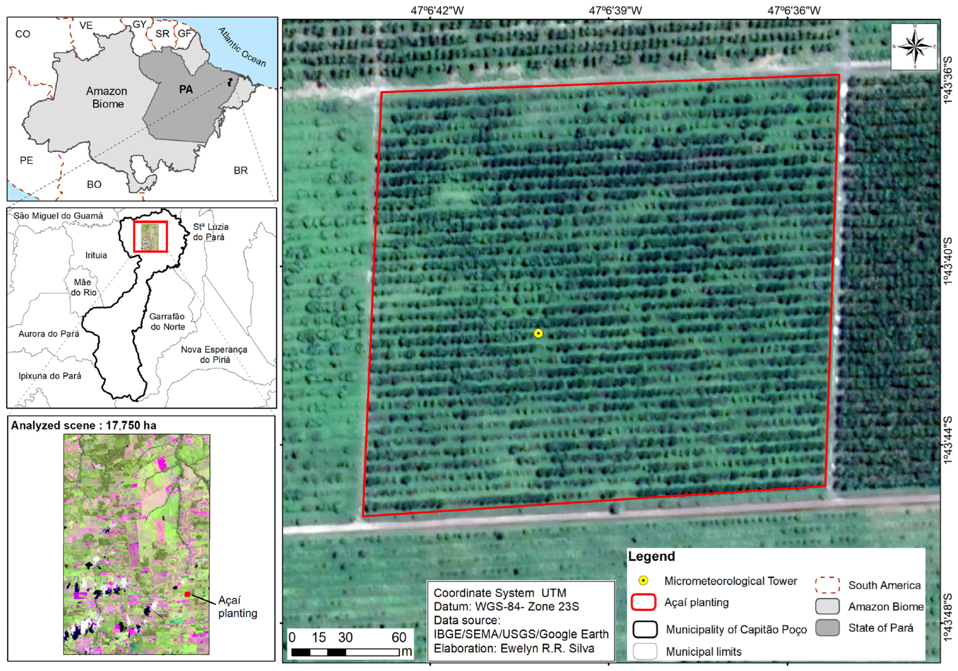
2.1. Study Area

The study was conducted in an area of 17,750 ha (Figure 1) in the municipality of Capitão Poço, belonging to the northeastern Paraense region of the eastern Legal Amazon. The rainy season of the region usually extends from December to June and the dry (less rainy) season from July to November [28].
The açaí was planted for commercial purposes in 2012 at Fazenda Ornela in the municipality of Capitão Poço. The planting spacing was 6.0 × 4.0 m, with three plants per clump, cultivated on dry land with daily irrigation, during the driest four months of the year (Aug–Nov), using a microaspersion system, where a gross empirical blade of 3.28 mm was applied daily. In 1 ha of the plantation, the field experiment was implemented (Figure 1), which was conducted during two açaizeiro harvests: the first from September 2017 to October 2018 and the second from November 2018 to October 2019.
In the experimental area, a 14 m high micrometeorological tower was installed (Figure 1), where three automatic meteorological data recorders that were distributed along the canopy (two from Campbell Scientific (Garbutt, Australia), model CR1000, and one from Onset Hobo (Bourne, MA, USA), model U30) were coupled. The system’s programming included reading the sensors every ten seconds and extraction of their averages every 20 min. The location of the tower obeyed the minimum requirements of area edge, presenting the available “fetch” (higher than the ratio 1:100), so that the obtained measurements were representative of the experimental area without the influence of advective energy [29]. Table 1 shows the sensors used in the experiment and their arrangement in relation to the soil or canopy. The data from the tower were used to compare the energy balance and evapotranspiration data estimated with the SEBAL algorithm.

2.2. Data from Landsat 8 Satellite Sensors

Six images generated by the Operational Land Imager (OLI) and Thermal Infrared Sensor (TIRS) of the Landsat 8 satellite were used, acquired free of charge from the United States Geological Survey (USGS) website which distributes both Landsat and other satellite data. For the selection of the satellite images, the data collection period of the micrometeorological tower was considered, as well as the least cloud interference in the analyzed scene (<10%), mainly at the micrometeorological tower site.
The days selected were 20 November and 22 December 2017 (orbit/point 222/61); 31 May (orbit/point 222/61) and 7 June (orbit/point 223/61) of 2018; and 26 June and 29 August 2019 (orbit/point 223/61), respectively, on Julian days 324, 356, 151, 158, 146, and 241. Initially, all OLI and TIRS sensor bands were stacked and cut out for the specific study area (açaí plot), before obtaining the different components of the radiation and energy balances.

2.3. Surface Energy Balance Algorithm for Land (SEBAL) Method

The latent heat flow (LE) (W m−2) was obtained according to Equation (1) [30]:
L E = R n G H
where R n is the balance of radiation, G is the heat flow in the ground, and H is the sensitive heat flow, with units in W m−2.
The balance of radiation (Rn) was obtained according to Bastiaanssen et al. [21]:
R n = R S 1 α s u p R L + R L 1 ε 0 R L
where R S is the incident shortwave radiation (W m−2); α s u p is the corrected surface albedo of each pixel; R L is the longwave radiation emitted from the atmosphere (W m−2); R L is the longwave radiation emitted from the surface (W m−2); and ε 0 is the emissivity of each pixel. The methodology proposed by Allen et al. [31] was followed to obtain α s u p , R L , R L , and ε.
The heat flow of the soil (G) (W m−2) was calculated according to the empirical equation developed by Bastiaanssen [30]:
G = T S 0.0038 + 0.0074 α 1 0.98 N D V I 4 R n
where T S is the surface temperature (°C), α is the surface albedo, and NDVI is the vegetation index of the normalized difference that was obtained through the following expression (Allen et al. [31]):
N D V I = r 4 r 5 r 4 + r 5
where r 4 and r 5 are the reflections corresponding to the near-infrared (band 5) and the red of the solar spectrum (band 4), respectively.
The values of the sensitive heat flow (H) were estimated based on the wind speed and the temperature difference (dT) near the surface between the levels in the atmosphere:
H = ρ c p d T r a h
where ρ is the specific mass of air (Kg m−3); c p is the specific heat of the air at constant pressure (1004 J kg−1 K−1); d T represents the temperature difference near the surface in Kelvin; and r a h is the aerodynamic resistance to heat transport (sm−1) between two heights near the surface (Z1 = 0.1 m and Z2 = 2.00 m).
The main hypothesis of the SEBAL model is to consider the existence of a linear relationship between the surface temperature difference and the air temperature, i.e., dT = a + b ∗ Ts. The obtaining of coefficients “a” and “b” demands the definition of two anchor pixels (hot and cold), which represent extreme conditions of temperature and humidity. The hot pixel was obtained in an area of exposed ground, with low NDVI and high values of temperature and albedo, where it was assumed that LE is null; therefore, H = Rn − G, and dT = H ∗ rah/ρ ∗ cp [30,32]. The cold pixel was obtained in an area with high vegetative vigor (high NDVI) and low temperature and albedo values, where H and dT were assumed to be null, and LE = Rn − G [30]. Such values of H were considered to initially serve only as input parameters of the iterative process in which they were used to identify the stability conditions of the atmosphere of each pixel according to the theory of similarity of Monin–Obukhov − L (m), computed according to Allen et al. [31]:
L = ρ c p u * 3 T s k g H
where ρ is the density of the air (1.15 kg m−3); cp is the specific heat of the air at constant pressure; u * is the speed of friction of each pixel of the images (m s−1); Ts is the temperature of the surface (K); g is the module of the terrestrial gravitational field (9.81 m s−2); and H is the flow of sensitive heat (W m−2), initially obtained considering the condition of neutrality. The values of L define the stability conditions as follows: when L < 0, the lower atmospheric limit layer is unstable, and when L > 0, the lower atmospheric limit layer is stable.
The values of the actual daily evapotranspiration (mm day−1) were obtained by extrapolation of the instantaneous value of LE (Equation (1)) in the daily value according to the methodology proposed by Bastiaanssen [30]:
E T 24 h = 0.035 L E R n G R s 24 h 1 α 110 τ s w 24 h
where R s 24 h is the daily global solar radiation (Wm−2), α is the surface albedo; τ s w 24 h is the daily average atmospheric transmittance, obtained as the ratio between the measured daily global solar radiation ( R n 24 h ) (MJ m−2) and the daily solar radiation incident at the top of the atmosphere ( R s t o a ) (MJ m−2); and 0.035 is the conversion factor from W m−2 to mm day−1.
The data of energy flows and evapotranspiration in the açaí plantation area were determined by indirect methods. The Bowen ratio method was used as proposed by Perez et al. [33]. Details about the experiment with Bowen’s ratio method can be found in Sousa et al. [6].

2.4. Algorithm Performance

For the performance evaluation of the algorithm, comparing the data observed in the field and the values estimated by the SEBAL algorithm, the methods of mean absolute error (MAE), mean relative error (MRE), the root of mean square error (RMSE), and the concordance index (d) developed by Willmott et al. [34] were used.
M A E = 1 N i = 1 N | E O |
M R E = 100 N i = 1 N | E O | O
R M S E = 1 N ( E O ) 2 N
d = 1 i = 1 n E i O i 2 i = 1 n | E i O ¯ | + | O i O ¯ | 2
where N is the number of pairs of the variables. E(Ei) and O(Oi) are, respectively, the values estimated by SEBAL and observed in the field for each variable evaluated. O ¯ is the overall mean of the observed values.
The MAE calculates the “mean absolute error” of errors between observations and simulations. The RMSE represents the root mean square of the errors between the observed values and those simulated by SEBAL with the same unit as the evaluated variable. Both statistical indices (MAE and RMSE) represent the average SEBAL error in relation to the observed data, and the lower their values, the better the estimate. The mean relative error (MRE) is defined as the ratio between the MAE and the value observed in the field. The MRE indicates how good the estimate is in relation to the magnitude of the observed variable; it is usually multiplied by 100 to express it as a percentage. Index d specifies the degree to which the observed deviations from Ō correspond, both in magnitude and sign, to deviations predicted by SEBAL from Ō. Values of index “d” close to 1 indicate an excellent agreement between the observed value and the simulated value, or that the error between them is small.

3. Results

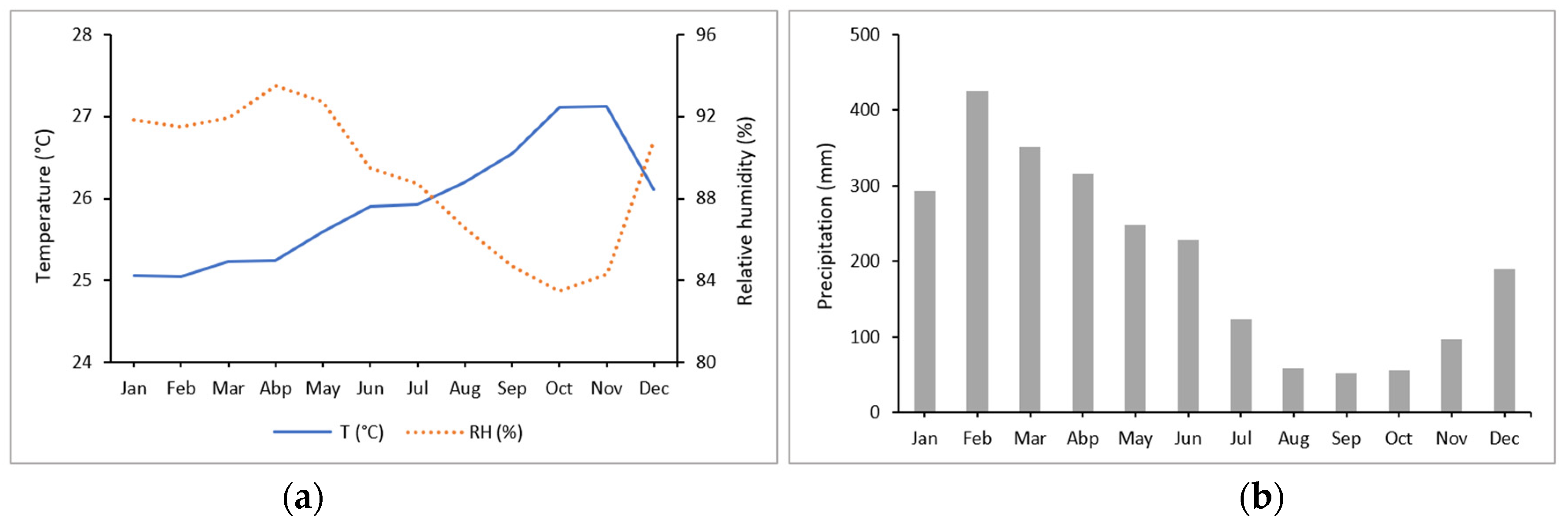
3.1. Weather Conditions

The variability of the monthly average air temperature and relative humidity of the data observed on the surface, for the period from September 2017 to November 2019, are represented in Figure 2a. The average air temperature during the studied period was 25.9 °C, oscillating between 25.1 °C and 27.2 °C, and the relative humidity of the air was an average of 89.1%, varying between 83.5% and 93.2%.
The total annual rainfall recorded in the study area for the same period was 2440 mm, where it was observed that the rainiest months were from January to June, with a peak in February (Figure 2b).
The information recorded by the sensors of the micrometeorological tower corresponding to the days analyzed in the Landsat 8 images, as well as information obtained from the metadata of the images, is shown in Table 2.
The daily global solar radiation ( R s 24 h ) varied between 20.3 and 22.6 MJ m−2, while the Rn varied between 12.7 and 15.5 MJ m−2. The maximum air temperature, obtained in the micrometeorological tower, was 32.5 °C and the minimum 29.3 °C. The relative humidity of the air showed variability between 66.5% on 20 November 2017 and 82.6% on 26 June 2019. The highest global instantaneous radiation recorded on the days evaluated at the moment of the satellite passage was 924.06 W m−2 on 20 November 2017 (DOY 324) followed by 844.67 W m−2 on 22 December 2017 (DOY 356). Despite this, the total R s 24 h on these two days did not follow the same trend, with lower Rn values compared to the other days.

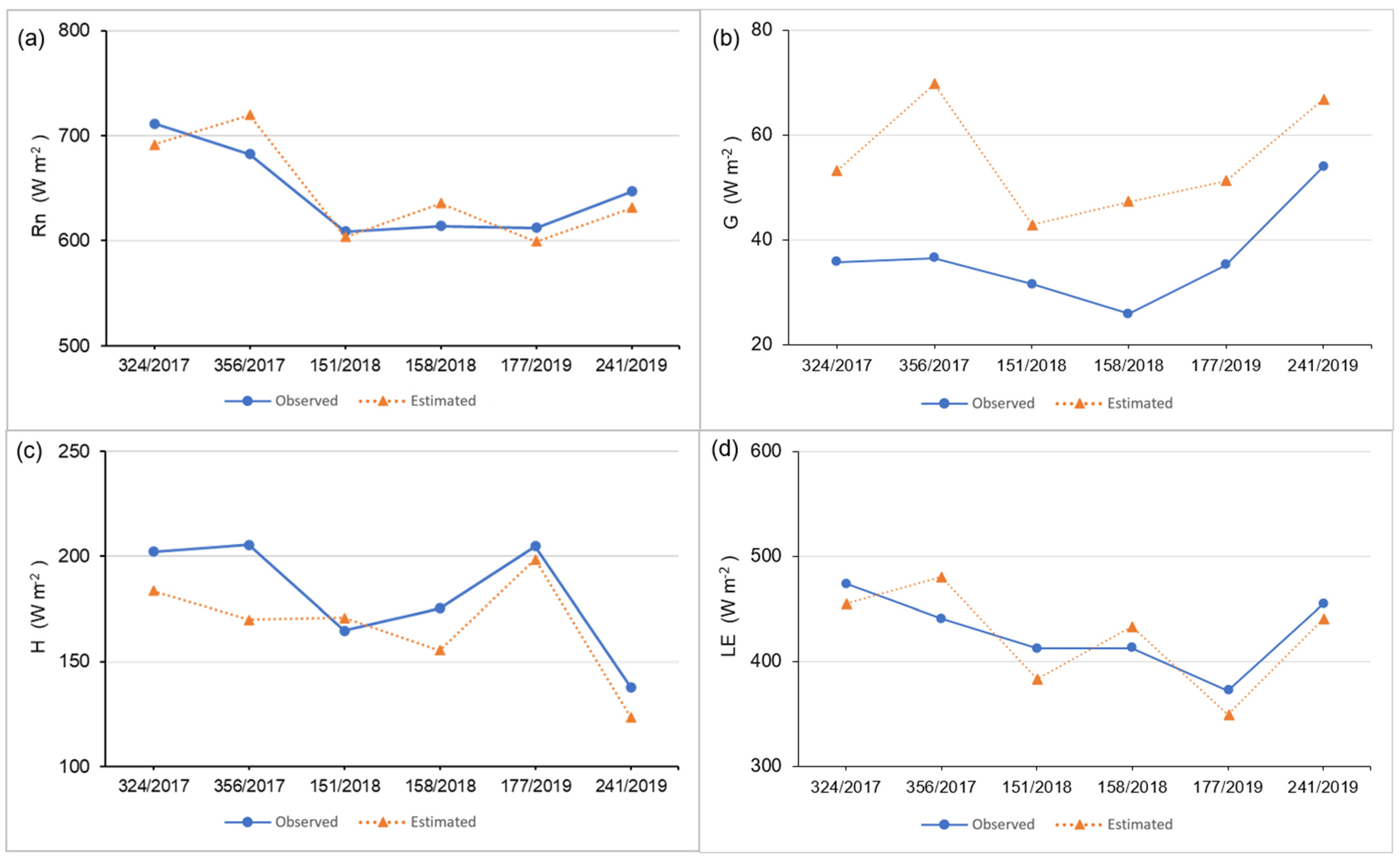
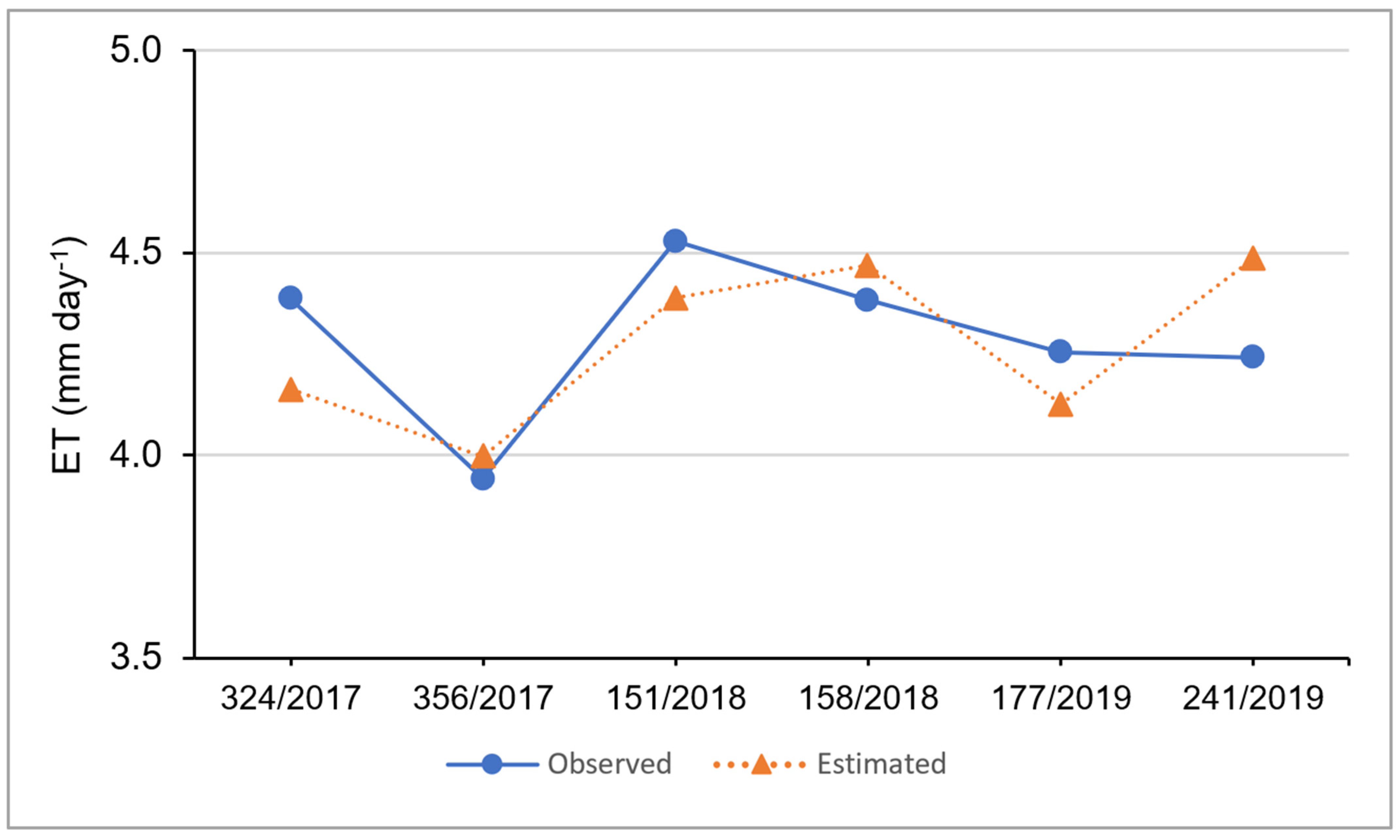
3.2. Comparison with Field Data

Figure 3 presents the values of energy flows obtained in the field through the micrometeorological tower installed in the açaí plantation area and the values estimated by the SEBAL algorithm at the time of the satellite passage.
For the radiation balance (Figure 3a), smaller differences were noticed between the estimated and observed values at the moment of the satellite passage, with an MRE of 2.84%, MAE of 18.65 W m−2, RMSE of 25.80 W m−2, and concordance index of 0.79 (Table 3).
For the heat flow in the soil (G), a greater discrepancy between the data was observed, mainly for 22 December 2017 (DOY 356) (Figure 3b), with the lowest index of agreement observed and errors equal to 64.42%, 20.81 W m−2, and 22.28 W m−2 for MRE, MAE, and RMSE, respectively (Table 3).
Among the energy balance variables, it can be observed that for the sensitive heat flow there was an overestimation on 31 May 2018 (DOY 151) (Figure 3c). For this component, the MRE was 9.89%, MAE was 17.97 W m−2, RMSE was 24.62 W m−2, and concordance index was 0.73 (Table 3).
Regarding the latent heat flow (Figure 3d), it was observed that the differences between the estimated and observed values were smaller too, similar to those observed for Rn. For LE, an MRE of 5.75%, MAE of 24.03 W m−2, RMSE of 31.14 W m−2, and d equal to 0.83 were obtained (Table 3).
Figure 4 shows the evapotranspiration values obtained in the micrometeorological tower and estimated by the SEBAL algorithm for the days analyzed.
Small differences were observed between the data estimated by SEBAL and those observed in the field, namely, the mean relative error, mean absolute error, root of the mean square error, and concordance index, equal to 4.23%, 0.45 mm dia−1, 0.52 mm dia−1, and 0.80, respectively (Table 3). It can be noted that the first days analyzed showed lower estimated and observed evapotranspiration values compared to the other days, although at the time of the satellite passage, the radiation balance (Figure 3a) and the latent heat flux (Figure 3d) resulted in possible high values.

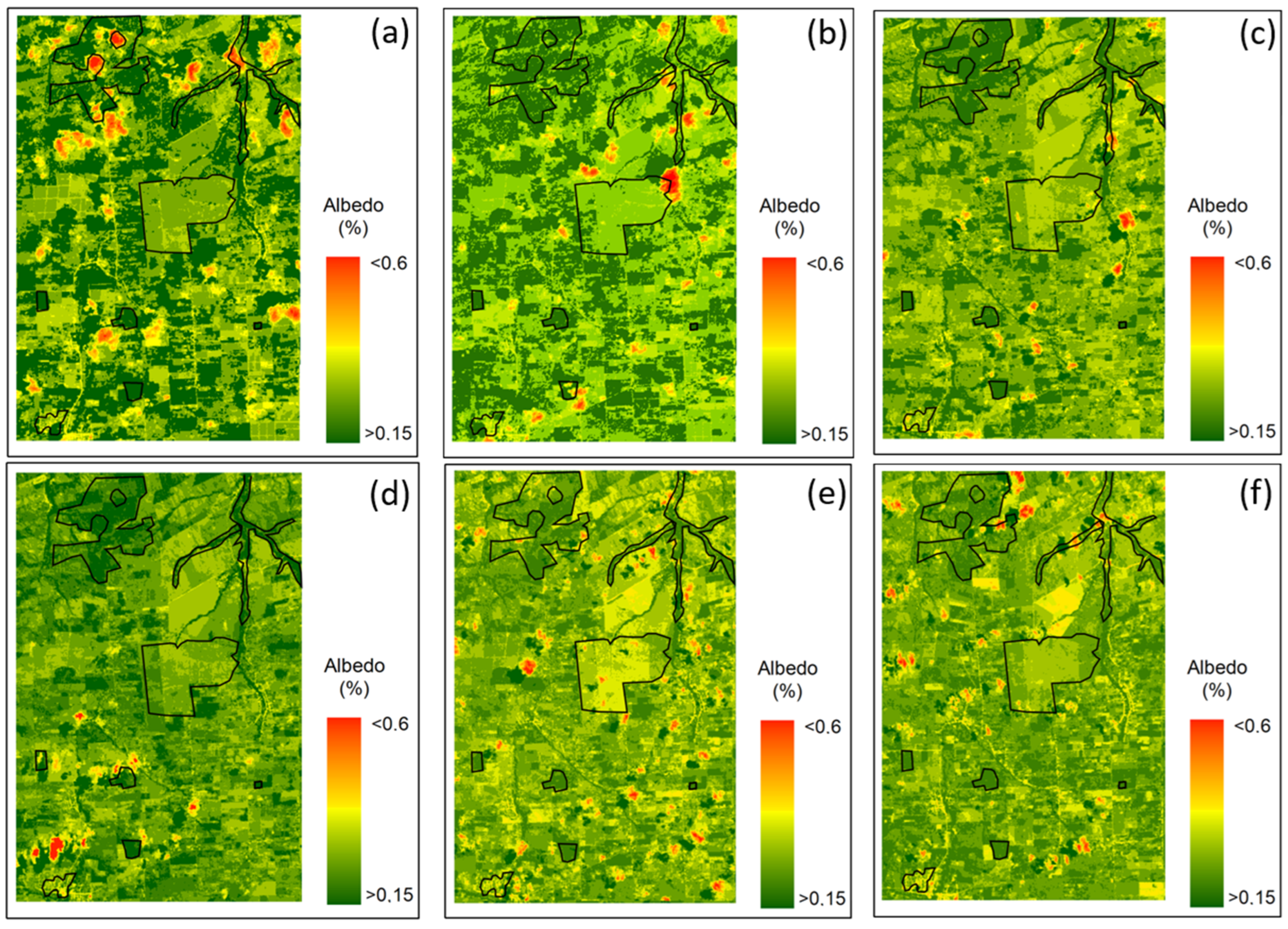
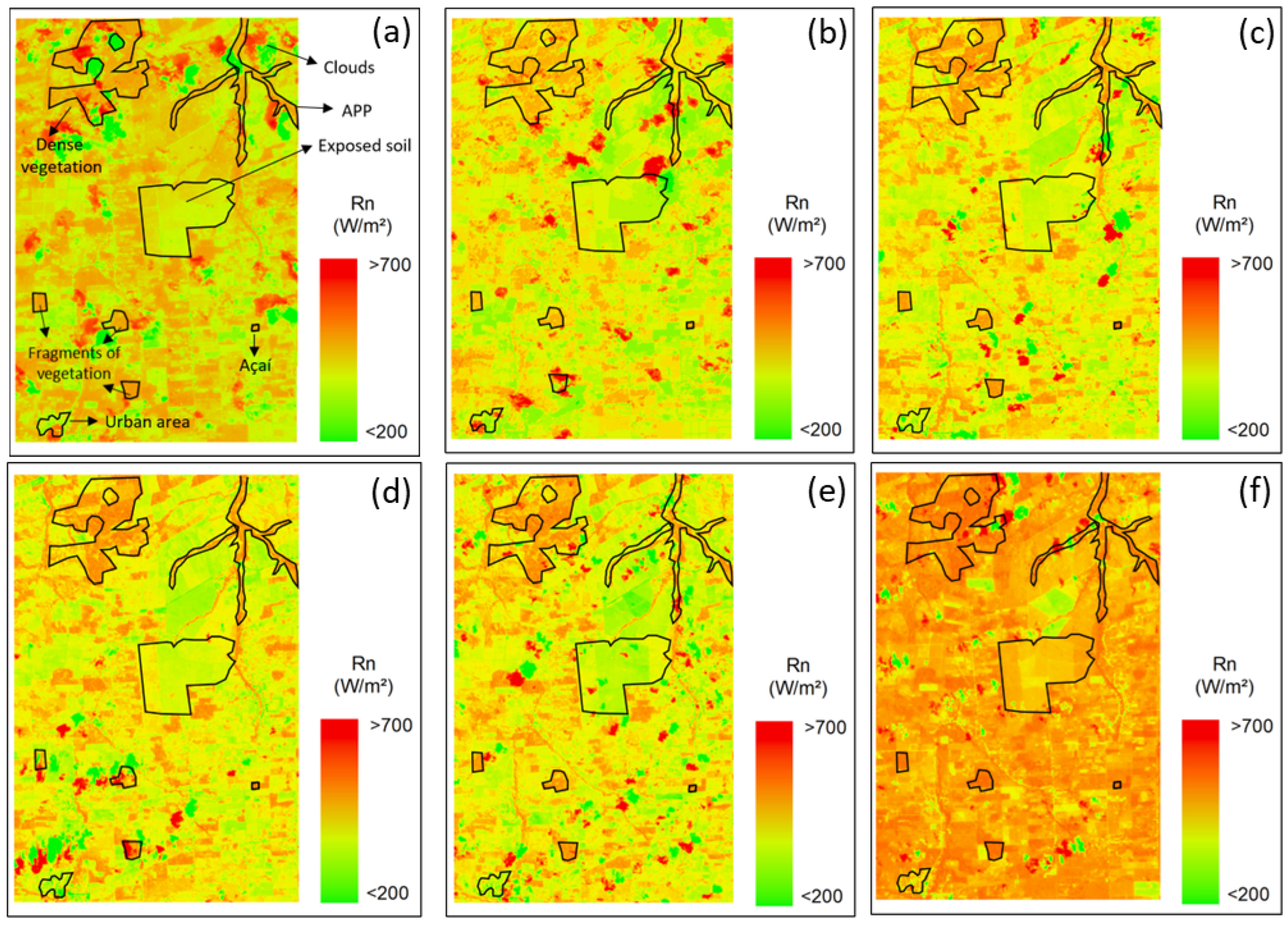
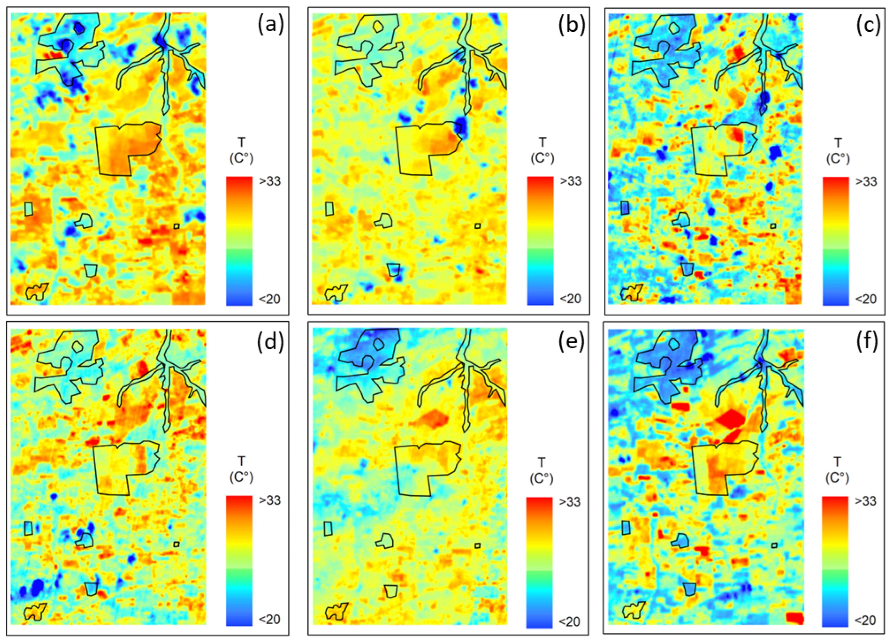
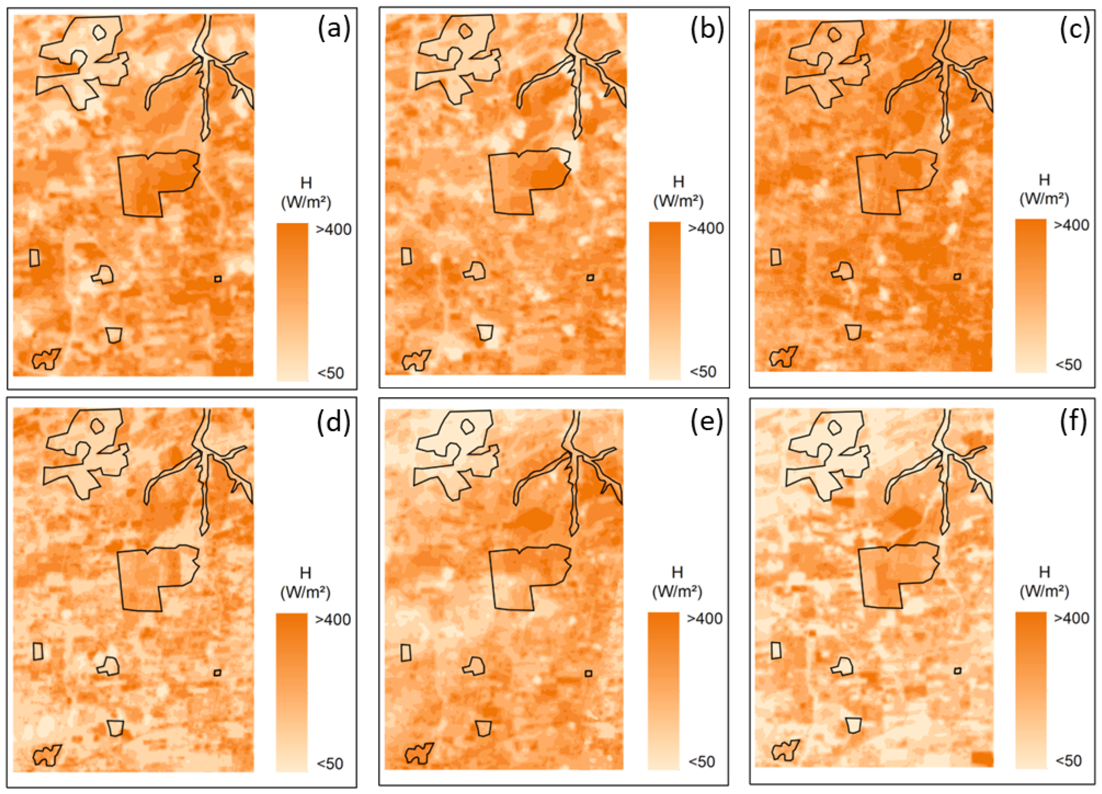
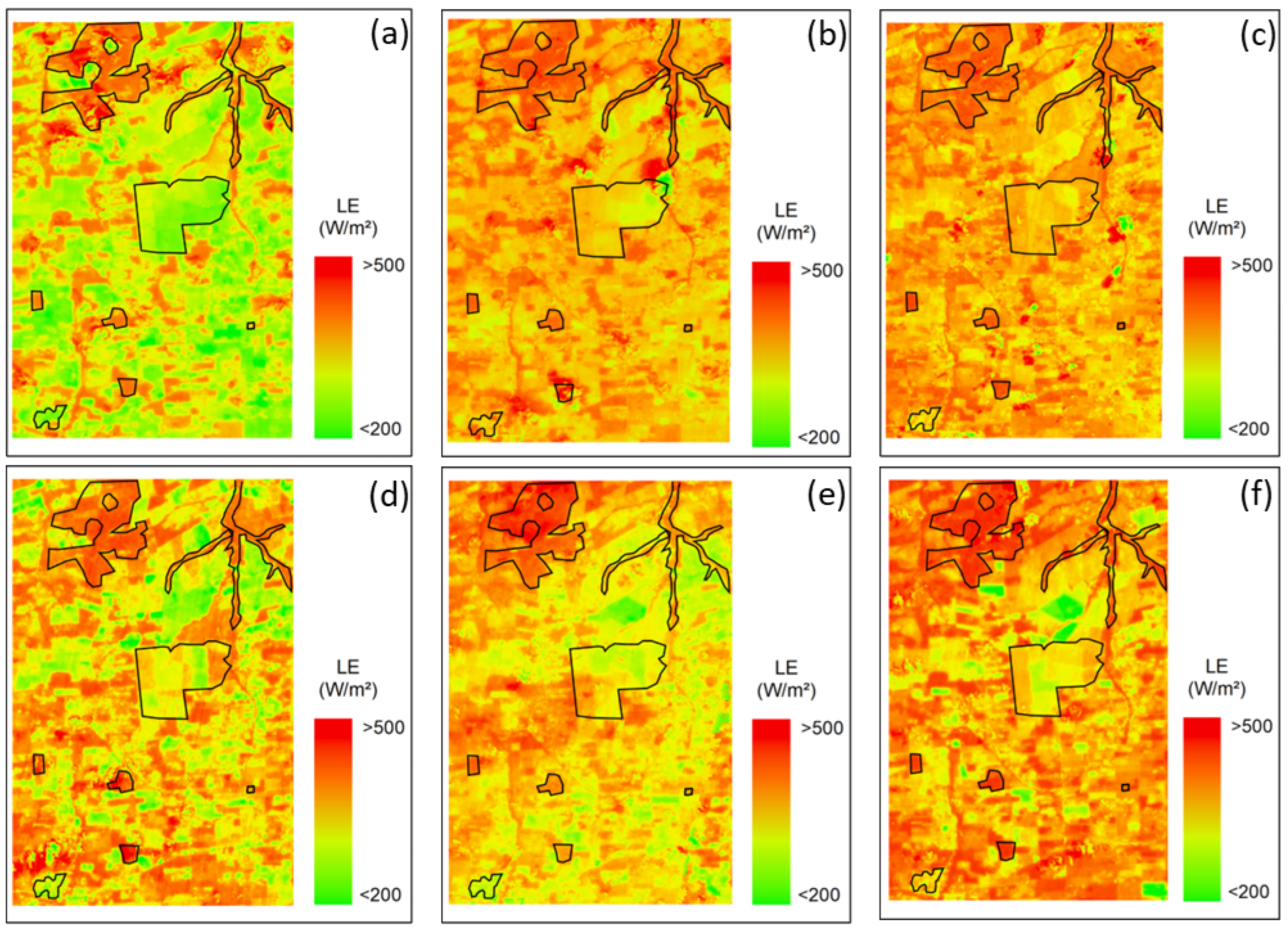
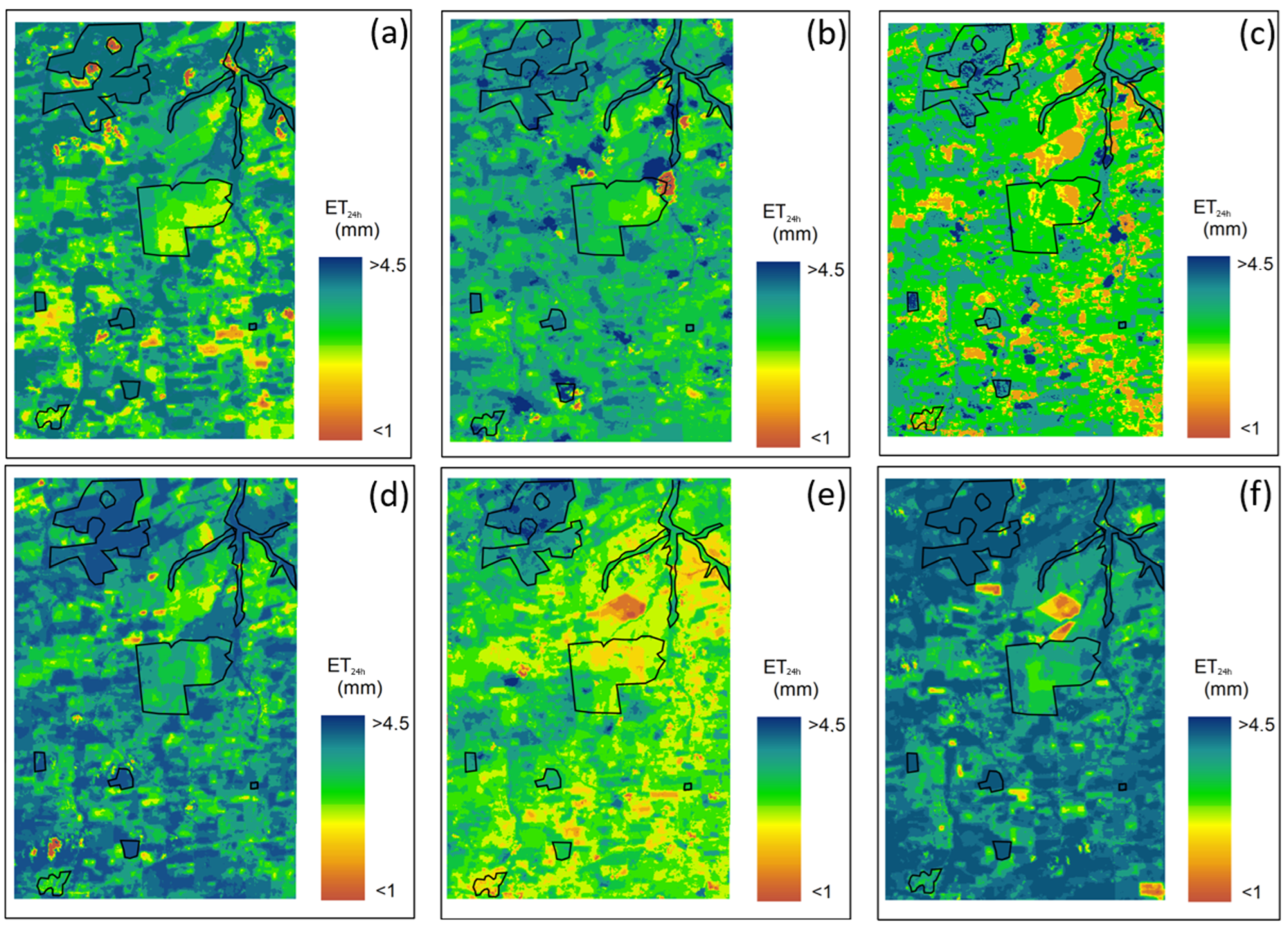
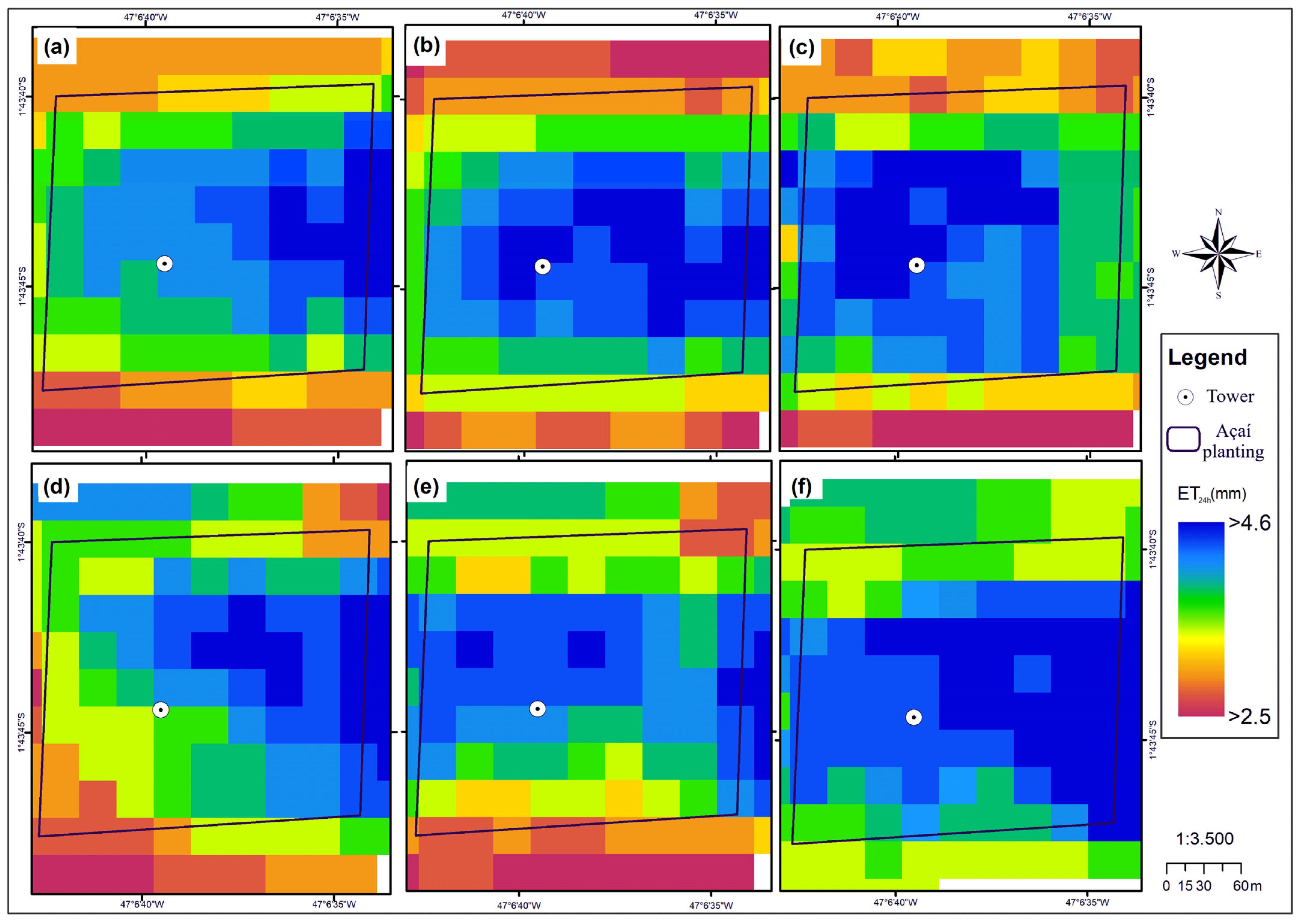
3.3. Spatialization of Energy Balance and Evapotranspiration Components

Figure 5, Figure 6, Figure 7, Figure 8, Figure 9 and Figure 10 represent the spatial distributions of the variables albedo ( α ) , radiation balance (Rn), surface temperature T , sensitive heat flow (H), latent heat flow (LE), and actual daily evapotranspiration ( E T 24 h ) , from 20 November 2017 (DOY 324) to 29 August 2019 (DOY 241).
Figure 5 shows the spatial variability of albedo from 20 November 2007 to 29 August 2019. The average albedo value for the whole scene on the first day evaluated was 0.22 (Figure 5a), and the maximum recorded in areas with exposed soil was 0.39. On 22 December 2017, the average value of albedo was 0.19 (Figure 5b). According to the scene analyzed on 31 May 2018 (Figure 5c), the average albedo of the area was 0.21, while in areas with exposed soil the values were between 0.29 and 0.35. The average value of the albedo was 0.18 on 7 June 2018, which varied in the area according to the type of surface coverage, foliar thickening of the plants, and incidence angle of the sun rays (Figure 5d). The albedo estimate at the point referring to the micrometeorological tower was 0.14 (Figure 5e). The average albedo of the scene obtained on 29 August 2019 was 0.19, and 0.16 at the point referring to the micrometeorological tower (Figure 5f).
For the Rn variable, it is noticed that in areas with exposed soil (in yellow on the map) the values of Rn ranged from 498.35 to 597.58 W m−2 (Figure 6a) on 20 November 2017 (the green color represents clouds in the image). On 22 December 2017, the Rn values that were between 530 and 641 W m−2 represent areas of exposed soil (Figure 6b). The average of the values for Rn was 629.61 Wm−2, with a maximum of 770 Wm−2. The average Rn was 575.1 W m−2 with a maximum value of 698.3 W m−2 on 31 May 2018 (Figure 6c). On 7 June 2018 (Figure 6d), the average Rn was 579.8 W m−2, with a maximum value of 694.63 W m−2. The data for 26 June 2019 is spatialized in Figure 6e. The average radiation balance was 585.28 W m−2 with the lowest observed value of 124.95 W m−2. On 29 August 2019, the radiation balance remained between 169.34 W m−2 and 734.49 W m−2 (Figure 6f).
On 20 November 2017, the estimated surface was highest from the central region down (Figure 7a). On 22 December 2017, during the rainy season, it was more stable (Figure 7b). The estimated temperature on 7 June 2018 varied from 20.07 °C to 32.3 °C with an average of 24.6 °C (Figure 7c). On 7 June 2018, the surface temperature estimate, at the point referring to the micrometeorological tower, was 25.6 °C (Figure 7d). The estimation obtained through the algorithm indicated a minimum surface temperature value of 22.3 °C and a maximum of 34.2 °C on 29 August 2019 (Figure 7f).
The maximum value for sensitive heat flow (H) was 429.29 W m−2 in the exposed soil area on 20 November 2017 (Figure 8a), while on 22 December 2017 this maximum value was equal to 528.4 W m−2 (Figure 8b). On 31 May 2018, the maximum value of H was 498.2 Wm−2 (Figure 8c), which was recorded in a place with less presence of vegetation cover and a higher temperature of 33.27 °C (Figure 7c). On 7 June 2018 (Figure 8d), the sensitive heat flow varied from 69.41 W m−2 to 509.12 W m−2, with an average value of 108.24 W m−2. The highest values of the sensitive heat flow were registered in areas with exposed soil on 26 June 2019 (Figure 8e); at the point referring to the tower, the H was 198.55 W m−2, and the average value for the analyzed scene was 187.09 W m−2. On 29 August 2019, the average value for the sensitive flows was 186.06 W m−2; for the micrometeorological tower point, this value was equal to 123.48 Wm−2 for H (Figure 8f).
The average value obtained for latent heat flow (LE) on 20 November 2017 was only 393,24 W m−2 (Figure 9a), less than the other periods evaluated. On 22 December 2017, the average value obtained for LE was 430.94 W m−2, with a maximum of 698 W m−2 in vegetated areas, indicating that most of the incident solar radiation is used by the plants in the evapotranspiration process as a form of latent heat (Figure 9b). An average of LE equal to 429.3 W m−2 and a maximum of 633.3 W m−2 were obtained in an area with vegetation fragments on 31 May 2018 (Figure 9c). On 7 June 2018, the LE estimates show an average of 452.91 W m−2 and a maximum of 733.78 W m−2 (Figure 9d). The highest values of latent heat flow obtained on 26 June 2019 are in areas with a higher density of vegetation (Figure 9e), and the maximum recorded reached a value of 558.92 W m−2. The average value for latent flows on 29 August 2019 was 468.69 W m−2; for the micrometeorological tower point, this value was equal to 441.17 Wm−2 (Figure 9f).
The daily evapotranspiration estimates over the period evaluated are presented in Figure 10. It was observed that in relation to heterogeneous soils the distribution of the daily value of ET was well distinguished by the model, with an average value for the scene of 3.64 mm day−1 on 20 November 2017 (Figure 10a). At the point where the micrometeorological tower was located, the ET estimated by SEBAL on this day was 4.16 mm day−1. In areas of surfaces covered with vegetation, it was observed that the ET was higher, reaching up to 6.45 mm in some areas, which also had high NDVI (>0.5) and low temperatures (Figure 7). The highest values of evapotranspiration were in areas with vegetal covering, namely, permanent preservation areas (APP) and fragments of dense vegetation (Figure 10b), as observed on 22 December 2017. On 31 May 2018, the mean ET value was 3.28 mm day−1 (Figure 10c) and the estimated ET in the açaí planting area was 4.39 mm day−1. The average value of ET on 7 June 2018 was 4.00 mm day−1, and at the site referring to the micrometeorological tower it was 4.47 mm day−1 (Figure 10d). On 26 June 2019, in areas with low vegetation the ET values were between 2.04 and 2.95 mm day−1, and the lowest estimates were in exposed soil areas (Figure 10e). On this day, the evapotranspiration value estimated in the açaí planting area was 4.13 mm day−1. Among all periods evaluated, the scene obtained from 29 August 2019 indicated a day with more available energy (Figure 6f) and latent flux (Figure 9f), and the evapotranspiration value in the açaí plantation was 4.49 mm day−1 (Figure 10f), while the average obtained for the analyzed scene was 4.14 mm day−1.
Figure 11 represents the spatial variability of evapotranspiration in the açaí plantation plot estimated with the SEBAL algorithm for the images analyzed in this study over the periods evaluated.
In the analysis of the recorded evapotranspiration values, a general average equal to 3.99 mm day−1 was observed, with a minimum average of 3.11 mm day−1 on 26 June 2019 (Figure 11e), and a maximum of 4.59 mm day−1 on 29 August 2019 (Figure 11f). The lowest value observed among the images was 2.70 mm day−1 on 26 June 2019; this value is below the empirical water slide used in the entire area by the owner (3.28 mm day−1). The maximum value was 4.89 on 29 August 2019 (Figure 11f).
The total evapotranspiration in the demarcated area estimated via remote sensing using SEBAL was 311.5 mm and 301.3 mm on days 324 and 356 of the year 2017 (Figure 11a,b, respectively), 364.1 mm and 339.1 mm for days 151 and 158 of the year 2018 (Figure 11c,d), and 253.0 mm and 371.6 mm for days 177 and 241 of 2019, respectively.
When considering the total evapotranspired water for the whole demarcated area based only on the value measured by the tower—equal to 4.39; 3.94; 4.53; 4.38; 4.25; and 4.24 mm day−1, respectively, with the totals respectively equal to 355.3; 319.3; 366.6; 355.0; 344.5; and 343.6 mm—it was possible to observe errors that varied from 0.7% to 26.6%, which can affect irrigation management and which demonstrate the importance of considering the existing spatial variability in the area.
Using the ETc estimated by SEBAL and the reference evapotranspiration (ETo) obtained from the automatic meteorological station of the National Institute of Meteorology (INMET), located 7 km from the experimental site, the simple crop coefficient (Kc) was obtained as the ratio of ETc to ETo and compared to the observed values for this açaí plantation plot found by Sousa et al. [6], according to Allen et al. [35] (Table 4).
It is noticed that SEBAL can be used to simulate the crop coefficient with good performance. The Kc values estimated by SEBAL range from 0.78 to 1.13, similar to the observed values (0.82 to 1.17). The Kc values simulated for the acai tree are similar to those of other perennial fruits, such as cacao and palm oil [35], which have Kc values ranging from 0.90 to 1.05. Additionally, it is noted that the variability observed in the field could be reproduced by the model, confirming its robustness and applicability in the region.

4. Discussion

4.1. Comparison with Field Data

The data in Table 2 indicate the climatic variability obtained in the study area. The lowest precipitation rates were in the period from July to November (Figure 2b). The maximum UR registered by the sensors of the micrometeorological tower was 82.6% on 26 June 2019. The municipality is located in a region subject to high rainfall at certain times of the year, which raises the relative humidity [36], as can be seen in Figure 2a.
According to Sousa et al. [6], the açaí tree in this region has two well-defined phases in well-defined seasons: the inflorescence phase predominates in the wettest period of the year (between November and March), while the inflorescence phase occurs in most of the rainy period and the beginning of the less rainy period (from March to October). The estimation of evapotranspiration during most of the infructescence phase is essential in supporting irrigation management due to the reduction in rainfall.
The available energy (Rn) values on the analyzed days were similar despite having been evaluated at different times of the year, and it was noticed that the average of the selected days in the year 2017 (DOY 324 and 356) was below the average of the other analyzed years (Table 2). The low values of Rn obtained for the 24 h period on days 324/2017 and 356/2017 are a consequence of the reduction in total solar radiation (Rs24h) recorded by the meteorological station after the moment of the satellite passage, which does not necessarily coincide with the pattern established at that moment (Rsinst).
Considering that SEBAL estimates the total evapotranspiration of the day as a function of the availability of energy in the form of latent heat from the evaporative fraction at the time of the satellite’s passage, the natural variability observed throughout the day is an important factor in determining the ETc. In spite of this small difference, the lower energy availability at the end of the year in this region is associated with the degree of cloudiness present in the atmosphere that causes a larger energy balance even in the winter period of the southern hemisphere [37].
The values estimated by the SEBAL algorithm were compared to the values coming from the micrometeorological tower at the moment of the satellite passage, as shown in Figure 3 and Table 3. For the radiation balance (Rn) (Figure 3a), higher values were estimated on 22 December 2017 and 7 June 2018, and these peaks may be related to the higher amount of clouds in these periods in the region. In tropical areas, the seasonal changes in cloud cover are the main influence on the incidence of solar radiation [28]. The Rn showed the lowest average relative error value among the energy flows and a good concordance index (Table 3). Similar results were found in different studies on radiation balance estimation using SEBAL, demonstrating the efficiency of the model for studies with this objective. Oliveira et al. [38], analyzing the liquid radiation in the Amazon in the southwest of the state of Pará, recorded RMSE ranging from 18.7 to 24.8 W m−2. Oliveira and Moraes [39] estimated and validated Rn in areas with pasture and forest characterizations in the central eastern portion of the state of Rondônia and obtained MRE errors of less than 3%.
In Ruhoff et al. [40], the error for the radiation balance was equal to 4% in studies on the estimation of evapotranspiration in the Rio Grande basin located in the tropical area of Cerrado. Good estimates of Rn using the SEBAL model were also found by Santos et al. [41] in the Jaru Biological Reserve in the Legal Amazon in the state of Rondônia, whose errors ranged from 7 to 16%. Thus, in this study, it is verified that the radiation balance estimate obtained by the SEBAL model in the analyzed area presented satisfactory results since, according to Ferreira et al. [15], for studies involving measurements and estimates of Rn with remote sensing, errors are expected to be small.
The greatest discrepancy between the values estimated by the algorithm and obtained at the surface was found for the heat flow in the soil (G) (Figure 3b), being the component which, when estimated with the aid of orbital images, presents greater uncertainties. The observed overestimation of this flow may be related to the effect that each canopy causes in the soil, sometimes working as a thermal insulator and reducing the radiation that reaches the surface [22], besides the fact that the measurements “in loco” are not always representative of the whole area [14]. However, this fact is not considered a limiting aspect of the model on a large scale, since the measurements of G “in loco” represent small areas, when the soil and vegetation cover are considered homogeneous [30]. Bastiaanssen et al. [21] affirm that the estimate of G via remote sensing is the one that presents the greatest difficulty due to the complexity in obtaining accurate data in the field. This also occurred in other studies, such as Timmermans et al. [42], who applied SEBAL in two experimental regions in Arizona and Oklahoma and obtained MAE and RMSE results equal to 24.0 W m−2 and 29.0 W m−2, respectively. Mendonça et al. [22], in the southeast region of Brazil, noticed significant overestimations of the heat flow in the soil above 60%. Monteiro et al. [43], in an irrigated soybean cultivation area in the municipality of Cruz Alta (RS), also obtained RMSE equal to 27.77 W m−2.
By analyzing the sensitive heat flow (H), it was observed that the model underestimated the observed data (Figure 3c); however, in relation to the methods used to evaluate the performance of the algorithm (Equations (8)–(11)), the results obtained were considered satisfactory (Table 3). The underestimation of variable H obtained in this study was also observed in Ruhoff et al. [40] in the Rio Grande basin between the states of São Paulo and Minas Gerais; these authors observed discrepancies in this component compared with surface data; however, the products obtained were acceptable. For Mendonça et al. [22] and Ruhoff et al. [40], the differences in the flow of sensible heat can be generated by the choice of pixel “anchors”; thus, after the creation of SEBAL, there were studies proposing different ways to choose these pixels, since this selection is subjective to each user and depends on each region in the study. For French et al. [44], these differences can be explained by a set of several factors relative to uncertainties and simplifications introduced in the algorithm, such as UR, Z 0 m , T a , a n d   ε a .
In Figure 3d, we have the values of latent heat flow (LE) at the moment of the satellite passage; the course of this flow follows the pattern of available energy (Rn), showing that most of the Rn, in the planting of açaí, is being directed to the evapotranspiration process of the plant. One of the factors that may have caused the minimum peaks observed on 31 May 2018 and 26 June 2019 is the low atmospheric demand in these periods, making the plant transpiration rate low. Field studies with other crops including palm trees also observed low rates of transpiration being caused, among other variables, by the contribution of atmospheric demand [45].
When comparing the data obtained in the açaí plantation with the results estimated by SEBAL, a good performance of the model was found for LE (Table 3). A similar result was found by Bhattacharya et al. [46] analyzing the estimate of regional evapotranspiration on agricultural land in India, with MRE and RMSE results equal to 22% and 28 W m−2, respectively. Relative errors between 3.8 and 9.6% were obtained by Bezerra, Silva, and Ferreira [32] when comparing castor bean and cotton crop data estimated with SEBAL with Bowen’s ratio method in the Cariri (EC) mesoregion. Bezerra et al. [25], in the semiarid region of northeastern Brazil, registered MAE, MRE, and RMSE equal to 19.4 W m−2, 4.4%, and 25.5W m−2, respectively.
The daily evapotranspiration (ET) estimation obtained by the SEBAL algorithm was similar to that observed in the field, calculated by Bowen’s ratio method (Figure 4), being the available energy that is converted and used by the plants in their evapotranspiration processes. It is noticed that the ETc on days 324/2017 and 356/2017 was lower than on the other days analyzed, although at the time of the satellite passage the energy available for the evaporation process was higher than in the rest of the period. This inverse behavior between Figure 3a,d and Figure 4 on the days in question corroborates the importance of total energy availability as one of the main determinants of evapotranspiration and not just the evaporative fraction established by the model at a given time of day.
The importance of determining the evapotranspiration of a crop, mainly in irrigated areas, is related to the determination of the water consumption by the plants and also to the irrigation blade that must be applied in the system [47], thus avoiding water losses. A good performance of the model was observed (Table 3); the errors associated with the ET component are acceptable (differences less than 15%) and in agreement with the literature on the application of remote sensing models for ET estimation [48]. It can be noted that this method offers the chance to assist producers in making decisions mainly concerning the irrigation of the cultivated area.
The study by Moreira, Adamatti, and Ruhoff [49], also in the Amazon region, showed errors ranging from 0.32 to 1.29 mm day−1, which demonstrates that the daily evapotranspiration values calculated by the algorithm were consistent when compared to “in loco” observations. Similar results were found by Silva et al. [23], in areas with coconut growing in the semiarid zone of the Brazilian Northeast, where the ET was estimated and presented an MAE, MRE, and RMSE equal to 0.43 mm day−1, 9.46%, and 0.53 mm day−1, respectively. In the analysis by Odi-Lara et al. [50], in a study carried out in a drip-irrigated apple orchard in Chile, the authors found promising results for the concordance index (0.90).
Oliveira et al. [24], estimating the ET in the Tapacurá river basin (PE), highlighted that despite the intense presence of clouds in the region the values obtained were considered satisfactory, with AMS, REQM, and ERM equal to 0.40 mm day−1, 0.51 mm day−1, and 9.63%, respectively, as in the analysis by Santos et al. [27]) in the northeastern region of Brazil, with REQM equal to 1.43 mm day−1. Silva et al. [26] obtained even more promising results for the municipality of Salto do Lontra (PR), with AMS equal to 0.3 mm day−1, demonstrating that the model obtained good estimates of evapotranspiration in the study area.

4.2. Spatialization of Energy Balance and Evapotranspiration Components

In areas with dense vegetation and ground vegetation, albedo values varied between 0.09 and 0.30 (Figure 5a–f). Because the denser vegetation has a darker color, it absorbs more solar radiation than the undergrowth and therefore has a lower albedo [51]. In these areas, most of the energy available to the environment is made available for the evapotranspiration process, cooling the vegetated surface [52].
In this study, the obtained average values in the analyzed scenes for the radiation balance (Rn) ranged from 575.10 W m−2 to 629.61 W m−2 (Figure 6). On the surface, the average value was around 646.09 W m−2. Also in northeast Pará, in a study by Freire et al. [53] carried out on a local scale analyzing the radiation balance in mangrove areas, averaged at 1:00 p.m., Rn was between 469 W m−2 and 572 W m−2. On the other hand, Souza, Rocha, and Ribeiro [37] obtained an average of 371.53 W m−2 in the harvest and between harvests of soybeans in eastern Amazonia. In the evaluated areas that had a low vegetation index or exposed soil, the radiation balance value (Rn) varied between 498.35 and 641.49 W m−2 (Figure 6a–f) and albedo between 0.17 and 0.45 (Figure 5a–f), which is related to an increase in the emission of terrestrial radiation resulting in lower Rn values.
Thus, an inversely proportional relationship is observed between these components (Rn and albedo) because the higher the coefficient of reflection, the more energy is reflected, and thus the lower the balance. The higher albedo values were already expected for the exposed soil areas, and in these same areas the estimated surface temperatures were higher (Figure 7a–f), confirming that the energy available to the environment is used for heating the soil and air adjacent to the surface in areas without vegetation cover, similar to the results obtained by Ferreira et al. [15] in exposed soil areas.
In the spatial distribution of the sensitive heat flow (H), shown in Figure 8a–f, it was verified that, in general, the smallest values of H correspond to small water bodies and areas of dense vegetation and vegetation fragments, with averages between 108.2 W m−2 and 187 W m−2 obtained. These values were low when compared with the study carried out at the local scale by Pereira and Rodrigues [54] in the municipality of Bragança, also in the northeast of the state of Pará, which found an average sensitive heat flow of 271.8 W m−2. The highest values of H were identified in areas of exposed soil, which had low NDVI (between 0.1 and 0.3), which was also reported by Ferreira et al. [15], in the Brazilian semiarid region, and by Mendonça et al. [22] in the northern region of Fluminense (RJ). These low rates of NDVI are related to the low vegetative vigor caused by the absence of vegetation; thus, a large part of the Rn is destined for the heating of the air in areas of exposed soil.
The highest values of latent heat flow (LE) (Figure 9a–f) correspond to areas with vegetation, with the red color representing areas with dense vegetation fragments, which also had high NDVI values, corroborating the methodology described in Allen, Tasumi, and Trezza [55]. There is a well-known and well-documented relationship between these areas with high NDVI values, i.e., areas with higher vegetation cover and lower surface temperature (Figure 7a–f), giving these areas a milder climate [56]. Thus, most of the available energy (Rn) in these areas is being directed to the transpiratory process of the plants in the form of LE consumption.
Figure 10a–f refer to the estimation of daily evapotranspiration (ET); the average estimated in the scenes was between 3.28 and 4.14 mm dia−1. The model was able to differentiate ET for the different types of ground cover since evapotranspiration is dependent on both atmosphere and surface parameters, that is, if there are changes in local parameters, this can cause variation in ET values. The highest ET values are in areas with dense vegetation, such as permanent preservation areas and vegetation fragments, which can be Legal Reserve Areas (LRAs), within the properties present in the analyzed area. The high vegetation indices (IAF > 3) found in these places explain the high values of evapotranspiration [47]. As açaí originates from floodplain areas with an abundance of water, the plant demands more water in the form of irrigation on firm ground; however, it is noted that in Figure 11 there are different values of evapotranspiration within the açaí plantation area itself, which would not make it necessary to standardize the use of a specific water blade for the entire area. This is noticeable in the analysis made in this study because currently the owner of the farm uses an empirical fixed slide of 3.28 mm day−1, which added together for the açaí plantation plot results in 265.68 mm day−1, but according to Figure 11e, for example, it results in 253.0 mm day−1.
Among the images analyzed, it was observed that higher ET values occurred on 29 August 2019 (Figure 11f) with a total evapotranspiration estimate equal to 371.6 mm for the delimited area of the açaí plot, an average of 4.49 mm day−1. This high value may be associated with the dry season in the region where there is not much rainfall and the temperatures are higher (Figure 7f), which contributes to a higher atmospheric demand (Table 4), which is eventually met due to the area receiving water through irrigation.
It is also verified that the values of ET inside the plot were greater than 3.0 mm day−1, except for on 26 June 2019 when a lower value was observed of 2.70 mm day−1 as well as a lower average of ET (3.11 mm day−1) (Figure 11e). These results can be explained by the high relative humidity of the air and the low temperature in this period in the region (Figure 3 and Table 2) because these variables comprise the climatic elements that help in the determination of the vapor pressure deficit, which is an indicator of the evaporative capacity of the air.
The variability found in the crop coefficients for açaí is due to the fact that the crop has different phases throughout the year, with a predominance of the inflorescence phase between November and March and the infructescence phase between March and October [6]. The days evaluated from the years 2017 and 2018 corresponded to the period in which the açaí tree was in the pre-flowering phase (DOY 324/2017 and 356/2017) and in the green fruit phase (DOY 151/2018 and 158/2018). According to Sousa et al. [6], the lower values of Kc during pre-flowering may be due to the transition from the less rainy season to the rainy season (Figure 1), when the amount of water in the soil is still a limiting factor, as well as the smaller leaf area of the acai tree due to the presence of new inflorescences located in the sheaths of the leaves which are released from the abscission of the leaves. The higher Kc in the green fruit stage may be associated with a better soil moisture level and a greater energy requirement for the crop to produce and dispose of photoassimilates for fruit growth and development, inducing a greater water demand by the plant [6].
Although the total estimate of the area presents differences (between 0.7 and 26.6%), it is important to remember that the values measured by the micrometeorological tower represent an estimate of an area at the windward side of the tower, and, considering the pattern adopted for the edge, represent a fetch of at least 200 m in the wind direction. These values represent the average evapotranspiration of the area but this unfortunately cannot be associated with the different pixels observed in the scenes used because it has not been monitored punctually with methodologies such as sap flow or water balance in the soil.
The value observed in the micrometeorological tower already indicates that the management adopted by the producer is inadequate to meet the water demand of the plant in the area, and, with the use of the SEBAL model, it was possible to corroborate this hypothesis for the spatial variability observed inside the plot of açaí (Figure 11). This fact demonstrates the importance of considering the spatial variability of the exchange processes existing in vegetated surfaces since the productivity to be reached is a reflection of the management adopted in the area, and, as shown in Figure 11, inside the plot there are areas with lower and higher water demand. Studies on the estimation of evapotranspiration in açaizeiro plantations using local methods and also using remote sensing are still scarce; however, it can be said that the methodology used in this study can bring satisfactory results for this purpose. Through the estimation of the energy balance with SEBAL, important information was obtained that can help producers to determine criteria for irrigation management as well as to establish the ideal water consumption of crops, thus reducing the expense of electric energy used for water pumping and reducing water waste.

5. Conclusions

The estimation of the energy balance components and the evapotranspiration by means of SEBAL applied to the OLI/TIRS sensor images of the Landsat 8 satellite are compatible with the data sets available on the açaí (Euterpe oleraceae M.) plantation surface.
The algorithm has good performance in determining the power fluxes H, LE, and Rn, with EAM equal to 17.97 W m−2, 24.03 W m−2, and 18.65 W m−2; ERM equal to 9.89%, 5.75%, and 2.84%; REQM equal to 24.62 W m−2, 31.14 W m−2, and 25.80 W m−2; and the concordance index equal to 0.73, 0.83, and 0.79, respectively.
Evapotranspiration (ET) presented good evaluation (ERM = 0.45 mm day−1, ERM = 4.23%, REQM = 0.52 mm day−1, and d = 0.80), which allows producers to use this methodology as an alternative to assist them in making decisions regarding irrigation management in cultivated areas, thus reducing expenses with energy costs and mainly water losses.
The results show the model’s potential to distinguish the different types of ground cover, demonstrating the sensitivity of the algorithm, which enabled the generation of maps of the distribution of the spatial and temporal variability of the components analyzed.

Author Contributions

Açaí experiment: P.J.d.O.P.d.S., E.R.R.S., D.d.P.S., D.B.d.L., H.G.G.C.N., G.S.T.F., J.V.d.N.P., V.D.d.S.F., I.A.d.O., S.A.S.d.S., J.F.C., M.L.R., D.L.P.C., V.B.M., M.J.A.d.L. and A.J.d.S.S.; conceptualization: P.J.d.O.P.d.S., E.R.R.S., B.B.d.S., T.R.F., M.A., A.M.L.d.S., J.E.O.S. and S.O.-F.; methodology: P.J.d.O.P.d.S., E.R.R.S., B.B.d.S., T.R.F., M.A., A.M.L.d.S., J.E.O.S. and S.O.-F.; software: E.R.R.S., B.B.d.S. and T.R.F.; data organization: P.J.d.O.P.d.S., E.R.R.S., D.d.P.S., D.B.d.L., H.G.G.C.N., G.S.T.F., J.V.d.N.P., V.D.d.S.F., I.A.d.O., S.A.S.d.S., J.F.C., D.L.P.C., V.B.M. and M.J.A.d.L.; data quality control: P.J.d.O.P.d.S., E.R.R.S., B.B.d.S., T.R.F., M.A., A.M.L.d.S., J.E.O.S. and S.O.-F.; data analysis: P.J.d.O.P.d.S., E.R.R.S., B.B.d.S., T.R.F., M.A., A.M.L.d.S., J.E.O.S. and S.O.-F.; writing—original draft preparation: P.J.d.O.P.d.S., E.R.R.S., B.B.d.S., T.R.F., M.A., A.M.L.d.S., J.E.O.S. and S.O.-F.; writing—review and editing: P.J.d.O.P.d.S., E.R.R.S., B.B.d.S., T.R.F., M.A., A.M.L.d.S., J.E.O.S. and S.O.-F.; project administration: P.J.d.O.P.d.S. and A.M.L.d.S.; funding acquisition: P.J.d.O.P.d.S. and A.M.L.d.S. All authors have read and agreed to the published version of the manuscript.

Funding

This research was funded by the National Council for Scientific and Technological Development (CNPq) through the Universal project (process no. 403902/2021-5), and by the Coordination for the Improvement of Higher Education Personnel—CAPES to the second author.

Data Availability Statement

Not applicable.

Acknowledgments

We would like to thank the rural producer Cid Ornela for making the experimental area of his farm available, and his employees for their support in the development of this research, and the Federal Rural University of the Amazon—UFRA, the Graduate Program in Agronomy—PgAgro, the Federal University of Campina Grande—UFCG, and the group Interaction Soil Plant Atmosphere in the Amazon—ISPAAM for logistics and for the support provided in this study. The authors acknowledge the Conselho Nacional de Desenvolvimento Científico e Tecnológico (CNPq) for the Research Productivity Fellowship of M. Adami (PQ—306334/2020-8), P.J.O.P. Souza (PQ—306728/2018-4).

Conflicts of Interest

The authors declare no conflict of interest. The funders had no role in the design of the study; in the collection, analyses, or interpretation of data; in the writing of the manuscript; or in the decision to publish the results.

References

  1. Elliott, J.; Deryng, D.; Müller, C.; Frieler, K.; Konzmann, M.; Gerten, D.; Glotter, M.; Flörke, M.; Wada, Y.; Best, N.; et al. Constraints and Potentials of Future Irrigation Water Availability on Agricultural Production under Climate Change. Proc. Natl. Acad. Sci. USA 2014, 111, 3239–3244. [Google Scholar] [CrossRef] [PubMed]
  2. Shrestha, S.; Bhatta, B.; Shrestha, M.; Shrestha, P.K. Integrated Assessment of the Climate and Landuse Change Impact on Hydrology and Water Quality in the Songkhram River Basin, Thailand. Sci. Total Environ. 2018, 643, 1610–1622. [Google Scholar] [CrossRef] [PubMed]
  3. Rosa, L.; Chiarelli, D.D.; Rulli, M.C.; Dell’Angelo, J. Global agricultual economic water scarcity. Sci. Adv. 2020, 6, eaaz6031. [Google Scholar] [CrossRef] [PubMed]
  4. Li, M.; Xu, Y.; Fu, Q.; Singh, V.P.; Liu, D.; Li, T. Efficient irrigation water allocation and its impact on agricultural sustainability and water scarcity under uncertainty. J. Hidrol. 2020, 586, 124888. [Google Scholar] [CrossRef]
  5. Sousa, F.F.; Vieira-Da-Silva, C.; Barros, F.B. The (in)Visible Market of Miriti (Mauritia flexuosa L.f.) Fruits, the ‘Winter Acai’ in Amazonian Riverine Communities of Abaetetuba, Northern Brazil. Glob. Ecol. Conserv. 2018, 14, e00393. [Google Scholar] [CrossRef]
  6. Sousa, D.D.P.; Fernandes, T.F.S.; Tavares, L.B.; Farias, V.D.D.S.; De Lima, M.J.A.; Nunes, H.G.G.C.; Costa, D.L.P.; Ortega-Farias, S.; Souza, P.J.D.O.P. Estimation of Evapotranspiration and Single and Dual Crop Coefficients of Acai Palm in the Eastern Amazon (Brazil) Using the Bowen Ratio System. Irrig. Sci. 2021, 39, 5–22. [Google Scholar] [CrossRef]
  7. Canalis-Ide, F.; Zubelzu, S.; Rodríguez-Sinobas, L. Irrigation systems in smart cities coping with water scarcity: The case of Valdebebas, Madrid (Spain). J. Environ. Manag. 2019, 247, 187–195. [Google Scholar] [CrossRef]
  8. Xu, G.; Xue, X.; Wang, P.; Yang, Z.; Yuan, W.; Liu, X.; Lou, C. A lysimeter study for the effects of different canopy sizes on evapotranspiration and crop coefficient of summer maize. Agric. Water Manag. 2018, 208, 1–6. [Google Scholar] [CrossRef]
  9. Paço, T.A.; Paredes, P.; Pereira, L.S.; Silvestre, J.; Santos, F.L. Crop Coefficients and Transpiration of a Super Intensive Arbequina Olive Orchard using the Dual Kc Approach and the Kcb Computation with the Fraction of Ground Cover and Height. Water 2019, 11, 383. [Google Scholar] [CrossRef]
  10. Domínguez-Niño, J.M.; Oliver-Manera, J.; Girona, J.; Casadesús, J. Differential irrigation scheduling by an automated algorithm of water balance tuned by capacitance-type soil moisture sensors. Agric. Water Manag. 2020, 228, 105880. [Google Scholar] [CrossRef]
  11. Xiong, Y.; Chen, X.; Tang, L.; Wang, H. Comparison of surface renewal and Bowen ratio derived evapotranspiration measurements in an arid vineyard. J. Hidrol. 2022, 613, 128474. [Google Scholar] [CrossRef]
  12. Martins, S.L.F.; Santos, M.A.; Lyra, G.B.; Souza, J.L.; Lyra, G.B.; Teodoro, I.; Ferreira, F.F.; Ferreira, R.A., Jr.; Almeida, A.C.S.; Souza, R.C. Actual Evapotranspiration for Sugarcane Based on Bowen Ratio-Energy Balance and Soil Water Balance Models with Optimized Crop Coefficients. Water Resour. Manag. 2022, 36, 4557–4574. [Google Scholar] [CrossRef]
  13. Bastiaanssen, W.G.M.; Noordman, E.J.M.; Pelgrum, H.; Davids, G.; Thoreson, B.P.; Allen, R.G. SEBAL Model with Remotely Sensed Data to Improve Water-Resources Management under Actual Field Conditions. J. Irrig. Drain. Eng. 2005, 6, 85–93. [Google Scholar] [CrossRef]
  14. Sarwar, A.; Bill, R. Mapping Evapotranspiration in the Indus Basin Using ASTER Data. Int. J. Remote Sens. 2007, 28, 5037–5046. [Google Scholar] [CrossRef]
  15. Ferreira, T.R.; Silva, B.B.; Moura, M.S.B.; Verhof, A.; Nobrega, R.L.B. The use of remote sensing for reliable estimation of net radiation and its components: A case study for contrasting land covers in an agricultural hotspot of the Brazilian semiarid region. Agric. For. Meteorol. 2020, 291, 188052. [Google Scholar] [CrossRef]
  16. Kool, D.; Kustas, W.P.; Ben-Gal, A.; Agam, N. Energy partitioning between plant canopy and soil, performance of the two-source energy balance model in a vineyard. Agric. For. Meteorol. 2021, 300, 108328. [Google Scholar] [CrossRef]
  17. Fuentes-Peñailillo, F.; Ortega-Farías, S.; Acevedo-Opazo, C.; Fonseca-Luengo, D. Implementation of a two-source model for estimating the spatial variability of olive evapotranspiration using satellite images and ground-based climate data. Water 2018, 10, 339. [Google Scholar] [CrossRef]
  18. Bwambale, E.; Abagale, F.K.; Anornu, G.K. Smart irrigation monitoring and control strategies for improving water use efficiency in precision agriculture: A review. Agric. Water Manag. 2022, 260, 107324. [Google Scholar] [CrossRef]
  19. Qiu, L.; Wu, Y.; Shi, Z.; Chen, Y.; Zhao, F. Quantifying the Responses of Evapotranspiration and Its Components to Vegetation Restoration and Climate Change on the Loess Plateau of China. Remote Sens. 2021, 13, 2358. [Google Scholar] [CrossRef]
  20. Jardim, A.M.R.F.; Araújo Junior, G.N.; Silva, M.V.; Santos, A.; Silva, J.L.B.; Pandorfi, H.; Oliveira-Junior, J.F.; Teixeira, A.H.C.; Teodoro, P.E.; Lima, J.L.M.P.; et al. Using Remote Sensing to Quantify the Joint Effects of Climate and Land Use/Land Cover Changes on the Caatinga Biome of Northeast Brazilian. Remote Sens. 2022, 14, 1911. [Google Scholar] [CrossRef]
  21. Bastiaanssen, W.G.M.; Menenti, M.; Feddes, R.A.; Holtslag, A.A.M. A Remote Sensing Surface Energy Balance Algorithm for Land (SEBAL) 1. Forlmutaion. J. Hydrol. 1998, 213, 198–212. [Google Scholar] [CrossRef]
  22. Mendonça, J.C.; De Sousa, E.F.; André, R.G.B.; Da Silva, B.B.; Ferreira, N.D.J. Estimativa Do Fluxo Do Calor Sensível Utilizando o Algoritmo SEBAL e Imagens MODIS Para a Região Norte Fluminense, RJ. Rev. Bras. Meteorol. 2012, 27, 85–94. [Google Scholar] [CrossRef]
  23. Silva, B.B.; Braga, A.C.; Braga, C.C.; De Oliveira, L.M.M.; Galvíncio, J.D.; Montenegro, S.M.G.L. Evapotranspiration and Assessment of Water Consumed in Irrigated Area of the Brazilian Semiarid Region by Remote Sensing|Evapotranspiração e Estimativa Da Água Consumida Em Perímetro Irrigado Do Semiárido Brasileiro Por Sensoriamento Remoto. Pesqui. Agropecu. Bras. 2012, 47, 1218–1226. [Google Scholar] [CrossRef]
  24. Oliveira, L.M.M.; Montenegro, S.M.G.L.; Da Silva, B.B.; Antonino, A.C.D.; De Moura, A.E.S.S. Evapotranspiração real em bacia hidrográfica do Nordeste brasileiro por meio do SEBAL e produtos MODIS. Rev. Bras. Eng. Agríc. Ambient. 2014, 18, 1039–1046. [Google Scholar] [CrossRef]
  25. Bezerra, B.G.; da Silva, B.B.; dos Santos, C.A.C.; Bezerra, J.R.C. Actual Evapotranspiration Estimation Using Remote Sensing: Comparison of SEBAL and SSEB Approaches. Adv. Remote Sens. 2015, 4, 234–247. [Google Scholar] [CrossRef]
  26. Silva, B.B.; Mercante, E.; Boas, M.A.V.; Wrublack, S.C.; Oldoni, L.V.; Melo, F.B.; Cardoso, M.J.; Júnior, A.S.A.; Ribeiro, V.Q. Satellite-Based ET Estimation Using Landsat 8 Images and SEBAL Model. Rev. Cienc. Agron. 2018, 49, 221–227. [Google Scholar] [CrossRef]
  27. Santos, C.A.C.; Mariano, D.A.; Nascimento, F.D.C.A.D.; Dantas, F.R.D.C.; de Oliveira, G.; Silva, M.T.; da Silva, L.L.; da Silva, B.B.; Bezerra, B.G.; Safa, B.; et al. Spatio-Temporal Patterns of Energy Exchange and Evapotranspiration during an Intense Drought for Drylands in Brazil. Int. J. Appl. Earth Obs. Geoinf. 2019, 85, 101982. [Google Scholar] [CrossRef]
  28. Moraes, B.C.; Da Costa, J.M.N.; Da Costa, A.C.L.; Costa, M.H. Variação Espacial e Temporal Da Precipitação No Estado Do Pará. Acta Amaz. 2005, 35, 207–214. [Google Scholar] [CrossRef]
  29. Rana, G.; Katerji, N. Measurement and Estimation of Actual Evapotranspiration in the Field under Mediterranean Climate: A Review. Eur. J. Agron. 2000, 13, 125–153. [Google Scholar] [CrossRef]
  30. Bastiaanssen, W.G.M. SEBAL-Based Sensible and Latent Heat Fluxes in the Irrigated Gediz Basin, Turkey. J. Hydrol. 2000, 229, 87–100. [Google Scholar] [CrossRef]
  31. Allen, R.G.; Tasumi, M.; Morse, A.; Trezza, R.; Wright, J.L.; Bastiaanssen, W.; Kramber, W.; Lorite, I.; Robison, C.W. Satellite-Based Energy Balance for Mapping Evapotranspiration with Internalized Calibration (METRIC)—Applications. J. Irrig. Drain. Eng. 2007, 133, 395–406. [Google Scholar] [CrossRef]
  32. Bezerra, B.G.; Da Silva, B.B.; Ferreira, N.J. Estimativa Da Evapotranspiração Real Diária Utilizando-Se Imagens Digitais TM—Landsat 5. Rev. Bras. Meteorol. 2008, 23, 305–317. [Google Scholar] [CrossRef]
  33. Perez, P.; Castellvi, F.; Ibáñez, M.; Rosell, J. Assessment of Reliability of Bowen Ratio Method for Partitioning Fluxes. Agric. For. Meteorol. 1999, 97, 141–150. [Google Scholar] [CrossRef]
  34. Willmott, C.J.; Ackleson, S.G.; Davis, R.E.; Feddema, J.J.; Klink, K.M.; Legates, D.R.; O’donnell, J.; Rowe, C.M. Statistics for the Evaluation and Comparison of Models. J. Geophys. Res. Ocean. 1985, 90, 8995–9005. [Google Scholar] [CrossRef]
  35. Allen, R.G.; Pereira, L.S.; Raes, D.; Smith, M. Crop Evapotranspiration: Guidelines for Computing Crop Water Requirements; Paper 56; FAO Irrigation and Drainage: Rome, Italy, 1998; 300p. [Google Scholar]
  36. Farias, V.D.S.; Costa, D.L.P.; Pinto, J.V.N.; Souza, P.J.O.P.; Souza, E.B.; Ortega-Farias, S. Calibration of reference evapotranspiration models in Pará. Acta Sci. 2020, 42, e42475. [Google Scholar] [CrossRef]
  37. Souza, P.J.D.O.P.D.; Da Rocha, E.J.P.; Ribeiro, A. Impacts of Soybean Expansion on Radiation Balance in Eastern Amazon. Acta Amaz. 2013, 43, 169–178. [Google Scholar] [CrossRef]
  38. Oliveira, G.; Brunsell, N.A.; Moraes, E.C.; Bertani, G.; Dos Santos, T.V.; Shimabukuro, Y.E.; Aragão, L.E.O.C. Use of MODIS Sensor Images Combined with Reanalysis Products to Retrieve Net Radiation in Amazonia. Sensors 2016, 16, 956. [Google Scholar] [CrossRef] [PubMed]
  39. Oliveira, G.; Moraes, E.C. Validação Do Balanço de Radiação Obtido a Partir de Dados MODIS/TERRA Na Amazônia Com Medidas de Superfície Do LBA. Acta Amaz. 2013, 43, 353–363. [Google Scholar] [CrossRef]
  40. Ruhoff, A.L.; Paz, A.R.; Collischonn, W.; Aragao, L.E.; Rocha, H.R.; Malhi, Y.S. A MODIS-Based Energy Balance to Estimate Evapotranspiration for Clear-Sky Days in Brazilian Tropical Savannas. Remote Sens. 2012, 4, 703–725. [Google Scholar] [CrossRef]
  41. Santos, C.C.D.; Nascimento, R.L.; Rao, T.V.R.; Manzi, A.O. Net Radiation Estimation under Pasture and Forest in Rondônia, Brazil, with TM Landsat 5 Images. Atmosfera 2011, 24, 435–446. [Google Scholar]
  42. Timmermans, W.J.; Kustas, W.P.; Anderson, M.C.; French, A.N. An Intercomparison of the Surface Energy Balance Algorithm for Land (SEBAL) and the Two-Source Energy Balance (TSEB) Modeling Schemes. Remote Sens. Environ. 2007, 108, 369–384. [Google Scholar] [CrossRef]
  43. Monteiro, P.F.C.; Fontana, D.C.; Santos, T.V.D.; Roberti, D.R. Estimativa dos componentes do balanço de energia e da evapotranspiração para áreas de cultivo de soja no sul do Brasil utilizando imagens do sensor TM Landsat 5. Bragantia 2014, 73, 72–80. [Google Scholar] [CrossRef]
  44. French, A.N.; Jacob, F.; Schmugger, T.J.; Kustas, W.P. TSEB vs. SEBAL: Comparison of two Surface Energy Flux Models. In Proceedings of the AGU Spring Meeting Abstracts, Washington, DC, USA, 28–31 May 2002; p. H51D-07. [Google Scholar]
  45. Passos, E.E.M.; Prado, C.H.B.A.; Aragão, W.M. The Influence of Vapour Pressure Deficit on Leaf Water Relations of Cocos Nucifera in Northeast Brazil. Exp. Agric. 2009, 45, 93–106. [Google Scholar] [CrossRef]
  46. Bhattacharya, B.; Mallick, K.; Patel, N.; Parihar, J. Regional Clear Sky Evapotranspiration over Agricultural Land Using Remote Sensing Data from Indian Geostationary Meteorological Satellite. J. Hydrol. 2010, 387, 65–80. [Google Scholar] [CrossRef]
  47. French, A.N.; Hunsaker, D.J.; Sanchez, C.A.; Saber, M.; Gonzalez, J.R.; Anderson, R. Satellite-based NDVI crop coefficients and evapotranspiration with eddy covariance validation for multiple durum wheat fields in the US Southwest. Agric. Water Manag. 2020, 239, 106266. [Google Scholar] [CrossRef]
  48. Carrasco-Benavides, M.; Ortega-Farías, S.; Lagos, L.O.; Kleissl, J.; Morales-Salinas, L.; Kilic, A. Parameterization of the Satellite-Based Model (METRIC) for the Estimation of Instantaneous Surface Energy Balance Components over a Drip-Irrigated Vineyard. Remote Sens. 2014, 6, 11342–11371. [Google Scholar] [CrossRef]
  49. Moreira, A.A.; Adamatti, D.S.; Ruhoff, A.L. Avaliação dos produtos de evapotranspiração baseados em sensoriamento remoto MOD16 e GLEAM em sítios de fluxos turbulentos do programa LBA. Ciência Nat. 2018, 40, 112. [Google Scholar] [CrossRef]
  50. Odi-Lara, M.; Campos, I.; Neale, C.M.U.; Ortega-Farías, S.; Poblete-Echeverría, C.; Balbontín, C.; Calera, A. Estimating Evapotranspiration of an Apple Orchard Using a Remote Sensing-Based Soil Water Balance. Remote Sens. 2016, 8, 253. [Google Scholar] [CrossRef]
  51. Zhang, X.; Jiao, Z.; Zhao, C.; Qu, Y.; Liu, Q.; Zhang, H.; Tong, Y.; Wang, C.; Li, S.; Guo, J.; et al. Statistics for the Evaluation and Comparison of Models. Remote Sens. 2022, 14, 1382. [Google Scholar] [CrossRef]
  52. Biudes, M.S.; Vourlitis, G.L.; Machado, N.G.; de Arruda, P.H.Z.; Neves, G.A.R.; Lobo, F.D.A.; Neale, C.M.U.; Nogueira, J.D.S. Patterns of Energy Exchange for Tropical Ecosystems across a Climate Gradient in Mato Grosso, Brazil. Agric. For. Meteorol. 2015, 202, 112–124. [Google Scholar] [CrossRef]
  53. Freire, A.S.; Vitorino, M.I.; Souza, A.M.L.; Germano, M.F. Analysis of the energy balance and CO2 fow under the infuence of the seasonality of climatic elements in a mangrove ecosystem in Eastern Amazon. Int. J. Biometeorol. 2021, 66, 647–659. [Google Scholar] [CrossRef] [PubMed]
  54. Pereira, P.L.; Rodrigues, H.J.B. Análise e Estimativa Dos Componentes Do Balanço de Energia Em Ecossistema de Manguezal Amazônico. Rev. Bras. Meteorol. 2013, 28, 75–84. [Google Scholar] [CrossRef]
  55. Allen, R.G.; Tasumi, M.; Trezza, R. SEBAL Surface Energy Balance Algorithms for Land: Advanced Training and Users Manual, Idaho Implementation, 1st ed.; Department of Water Resources, University of Idaho: Moscow, ID, USA, 2002.
  56. Fayech, D.; Tarhouni, J. Climate variability and its efect on normalized diference vegetation index (NDVI) using remote sensing in semiarid area. Model. Earth Syst. Environ. 2021, 7, 1667–1682. [Google Scholar] [CrossRef]
Figure 1. Location of the study area and the micrometeorological tower in the açaí plantation.
Water 15 01073 g001
Figure 2. (a) Average monthly temperature and relative humidity and (b) average total monthly precipitation from September 2017 to November 2019.
Water 15 01073 g002
Figure 3. Comparison of the components of the energy balance between the data estimated by SEBAL and observed at the surface: (a) radiation balance (Rn); (b) heat flow in the soil (G); (c) sensitive heat flow (H); and (d) latent heat flow (LE).
Water 15 01073 g003
Figure 4. Evapotranspiration values of the micrometeorological tower data and the data estimated by SEBAL.
Water 15 01073 g004
Figure 5. Temporal distribution of albedo (α) on 20 November 2017 (a), 22 December 2017 (b), 31 May 2018 (c), 7 June 2018 (d), 26 June 2019 (e), and 29 August 2019 (f).
Water 15 01073 g005
Figure 6. Temporal distribution of radiation balance (Rn) on 20 November 2017 (a), 22 December 2017 (b), 31 May 2018 (c), 7 June 2018 (d), 26 June 2019 (e), and 29 August 2019 (f).
Water 15 01073 g006
Figure 7. Temporal distribution of the variable surface temperature (T) on 20 November 2017 (a), 22 December 2017 (b), 31 May 2018 (c), 7 June 2018 (d), 26 June 2019 (e), and 29 August 2019 (f).
Water 15 01073 g007
Figure 8. Temporal distribution of the sensitive heat flow (H) on 20 November 2017 (a), 22 December 2017 (b), 31 May 2018 (c), 7 June 2018 (d), 26 June 2019 (e), and 29 August 2019 (f).
Water 15 01073 g008
Figure 9. Temporal distribution of latent heat flow (LE) on 20 November 2017 (a), 22 December 2017 (b), 31 May 2018 (c), 7 June 2018 (d), 26 June 2019 (e), and on 29 August 2019 (f).
Water 15 01073 g009
Figure 10. Temporal distribution of actual daily evapotranspiration (ET24h) on 20 November 2017 (a), 22 December 2017 (b), 31 May 2018 (c), 7 June 2018 (d), 26 June 2019 (e), and 29 August 2019 (f).
Water 15 01073 g010
Figure 11. Spatial variability in evapotranspiration estimation in açaí planting area on the analyzed days: (a) 20 November 2017(DJ 324); (b) 22 December 2017 (DOY 356); (c) 31 May 2018 (DOY 151); (d) 7 June 2018 (DOY 158); (e) 26 June 2019 (DOY 177); (f) 29 August 2019 (DOY 241).
Water 15 01073 g011
Table 1. Variables and instruments used in the experiment, as well as their arrangement in relation to the soil and the plant canopy.
Weather VariablesInstrument and ModelSensor Level (m)
Air temperatureVaisala thermohygrometer (HMP35A)2 and 8 above the ground
Relative humidityVaisala thermohygrometer (HMP35A)2 and 8 above the ground
Air temperature Hobo (STHB-M002)0.5 and 2 above the canopy
Relative humidityHobo (STHB-M002)0.5 and 2 above the canopy
Soil moistureTime Domain Reflectometer (CS615)−0.3 soil surface
RainRain gauge (TB4-L)0.5 above the canopy
Global incident radiationPyranometer (CMP6-L)2 above the canopy
Balance of radiationNet Radiometer (NR-LITE2-L)2 above the canopy
Ground heat flowSoil Heat Flux Plate (HFP01SC-L)−0.08 soil surface
Wind speed and directionWind Monitor (05106-L)2 above the canopy
Table 2. R s 24 h : total daily global solar radiation (MJ m−2); R n : total daily radiation balance (MJ m−2); Ta: air temperature at the moment of the satellite passage (°C); RH: relative humidity at the moment of the satellite passage (%); R s i n s t : instantaneous global radiation at the moment of the satellite passage (W m−2); τ s w : atmospheric transmissivity at the moment of the satellite passage; cosZ: cosine of the solar zenith angle at the moment of the satellite passage.
DOY *   R s 24 h *   R n *   Ta *   RH *   R s i n s t τ s w cosZ
324/201722.613.632.566.5924.060.7220.871
356/201720.312.731.372.5844.670.7210.829
151/201822.015.229.679.6776.360.7060.817
158/201821.214.729.476.7766.940.7090.810
177/201921.915.329.382.6774.030.7030.801
241/201922.215.530.274.6645.980.7170.872
Note: * Data recorded by sensors in the micrometeorological tower.
Table 3. The average absolute error, average relative error, root of the average quadratic error, and concordance index between the energy balance and evapotranspiration variables.
RnGHLEET24h
MAE (W m−2)18.65 20.81 17.97 24.030.45 (mm day−1)
MRE (%)2.84 64.42 9.89 5.75 4.23
RMSE (W m−2)25.80 22.28 24.62 31.14 0.52 (mm dia−1)
d0.790.470.730.830.80
Table 4. Reference evapotranspiration (ETo), crop evapotranspiration (ETc), and single crop coefficient (Kc) estimated by SEBAL and observed in field.
DOY E T o E T c _ E ETc_OKc_E K c _ O
324/20175.364.164.440.780.83
356/20174.224.003.990.940.95
151/20183.884.394.531.131.17
158/20184.084.474.381.091.07
177/20195.134.134.520.800.88
241/20195.614.494.590.800.82
Disclaimer/Publisher’s Note: The statements, opinions and data contained in all publications are solely those of the individual author(s) and contributor(s) and not of MDPI and/or the editor(s). MDPI and/or the editor(s) disclaim responsibility for any injury to people or property resulting from any ideas, methods, instructions or products referred to in the content.

