Article

Forecasting Monthly Water Deficit Based on Multi-Variable Linear Regression and Random Forest Models

1
Key Laboratory of Agricultural Soil and Water Engineering in Arid and Semiarid Areas at Ministry of Education, College of Water Resources and Architecture Engineering, Northwest A & F University, Xianyang 712100, China
2
State Key Laboratory of Simulation and Regulation of Water Cycle in River Basin, China Institute of Water Resources and Hydropower Research, Beijing 100038, China
3
College of Water Conservancy & Architectural Engineering, University Shihezi, Shihezi 832003, China
4
NSW Department of Primary Industries, Wagga Wagga Agricultural Institute, Wagga Wagga, NSW 2650, Australia
5
College of Land Science and Technology, China Agricultural University, Beijing 100193, China
*
Authors to whom correspondence should be addressed.
These authors contributed equally to this work.
Water 2023, 15(6), 1075; https://doi.org/10.3390/w15061075
Submission received: 3 February 2023 / Revised: 3 March 2023 / Accepted: 7 March 2023 / Published: 10 March 2023
(This article belongs to the Special Issue Environmental and Human Impacts on Hydrological Drought)

Abstract

:
Forecasting water deficit is challenging because it is modulated by uncertain climate, different environmental and anthropic factors, especially in arid and semi-arid northwestern China. The monthly water deficit index D at 44 sites in northwestern China over 1961−2020 were calculated. The key large-scale circulation indices related to D were screened using Pearson’s correlation (r). Subsequently, we predicted monthly D with the multi-variable linear regression (MLR) and random forest (RF) models at certain lagged times after being strictly calibrated and validated. The results showed the following: (1) The r between the monthly D and the screened key circulation indices varied from 0.71 to 0.85 and the lagged time ranged from 1 to 12 months. (2) The calibrated and validated performance of the established MLR and RF models were all good at the 44 sites. Overall, the RF model outperformed the MLR model with a higher coefficient of determination (R2 > 0.8 at 38 sites) and mean absolute percentage error (MAPE < 50% at 30 sites). (3) The Pacific Polar Vortex Intensity (PPVI) had the greatest impact on D in northwestern China, followed by SSRP, WPWPA, NANRP, and PPVA. (4) The forecasted monthly D values based on RF models indicated that the water deficit in northwestern China would be most severe (−239.7 to −62.3 mm) in August 2022. In conclusion, using multiple large-scale climate signals to drive a machine learning model is a promising method for predicting water deficit conditions in northwestern China.

1. Introduction

The sixth comprehensive report of the Intergovernmental Panel on Climate Change pointed out that the global climate would further warm up in the future. Global warming triggers anomalous climate and circulation [1], and changes the relative values of precipitation and evapotranspiration, which denotes water deficit and surplus conditions [2]. Influenced by climate change, the anomalous water deficit at the land–atmosphere interface is directly connected with lower precipitation and higher evapotranspiration than normal [3], which often leads to extreme events such as drought, flooding, and rainstorm. Water deficit has impacted the severity, frequency, and magnitude of the drought hazards and imposed severe threats to ecosystems, human societies, and civilization [4]. The occurrence and formation of drought disasters not only involve complex dynamic processes with multiscale water-energy cycle mechanisms, but also meteorology, agriculture, hydrology, ecology, socioeconomics, and other fields. Due to the great perniciousness, the research related to prediction of water deficit (or drought hazards) is very important [5].
Water deficit is the result of the insufficient precipitation and subsequent soil water and plant water loss, which are mainly reflected by soil evaporation and plant transpiration (i.e., evapotranspiration) [6]. There are different types of evapotranspiration including potential evapotranspiration, reference crop evapotranspiration (ET0), pan evaporation, and actual evapotranspiration. The difference of precipitation and ET0 (denoted as D here and after) characterizes water deficit very well and further was used for computing drought indices, e.g., standardized precipitation and evapotranspiration index (SPEI) [7]. Water deficit is a natural feature of climate and occurs in almost all climate regions, and it varies in frequency, severity, and duration. For example, Mihăilă et al. [8] investigated the temporal and spatial trends of D between the Carpathian Mountains and the Dniester River over 1961−2012. They pointed out that the climate of the region underwent an evolution process to a more arid climate. Das et al. [9] analyzed the drought patterns in India using D over 1901−2008. They found that in eastern India, the increase in drought events was attributed to decrease in rainfall, while in the arid areas of the west, the decrease in drought events was mainly due to increase in rainfall. In addition, some researchers analyzed the spatiotemporal changes of drought on the basis of drought index calculated by D. Somorowska et al. [10] analyzed the changes of drought situation in Poland over 1956−2015 using SPEI at 3, 6, and 12 months and found that the severity of droughts from southwestern to central Poland increased. Additionally, drought events of different severity occurred in winter and summer. These studies demonstrated that D can be well used to monitor and evaluate the long-term dry and wet conditions.
Climate change and human activities are major drivers of water deficit. Human activity drivers refer to irrigation, human water use, the modification of land use/land cover, urbanization and industrialization, etc., which have significant impacts on water resources [11]. Excessive human activities will lead to land degradation and severe ecological and environmental problems, and drought on degraded land and regions will show a positive feedback effect, making more severe drought conditions. For example, Jiang et al. [12] investigated the impact of climate change and human activities on hydrological drought using the fixed runoff threshold level and standardized runoff index in the Laohahe catchment in North China. They found that human activities were the dominant factor affecting hydrological drought with an upward trend. Climate change drivers refer to circulation, precipitation, temperature, water vapor transport, pressure belts and wind belts, etc. Of these, circulations have played vital roles in affecting water deficit conditions. The potential relationship of large-scale climate signals affecting remote areas through circulation is called teleconnection. Teleconnection is an important part of climate drive, and its essence is low-frequency, repetitive, continuous, large-scale pressure and circulation abnormal patterns [13]. Circulation indices, along with drought indices, were used for teleconnection analysis between water deficit (or drought) and circulations. For example, Özger et al. [14] applied wavelet transform and kriging to investigate the spatial structure of the teleconnection between El Niño Southern Oscillation (ENSO)/Pacific Decade Oscillation (PDO) and the palmer drought severity index in the 20th century. It was worth noting that arid regions were more closely related to climate anomalies than tropical humid regions. Talaee et al. [15] linked ENSO with the standardized streamflow index in western Iran over 1969−2009, noting that extreme and severe hydrological drought events in western Iran’s hydrological years were strongly correlated with ENSO. Manzano et al. [16] assessed the teleconnection between SPEI and large-scale circulation factors in the Iberian Peninsula. They concluded that Artic Oscillation (AO) and North Atlantic Oscillation (NAO) patterns had significant impacts on droughts in winter over large areas of the Iberian Peninsula. Previous research found that there were potential connections between water deficit and circulation at regional or global scales.
Many statistical models have been used to estimate hydro-meteorological variables with different circulation indices. For example, Esha and Imteaz [17] evaluated the potential of several circulation factors to predict long-term runoff using the MLR technique in New South Wales. They found that the Pearson’s correlation coefficient (r) of established MLR models at all 12 sites showed good results (r = 0.51–0.65). Acharya et al. [18] used the MLR model to predict the standardized precipitation index (SPI) in India with nine general circulation model products. They showed that the ability of the atmosphere-ocean coupled models was better than the atmospheric models. The multi-variable linear regression (MLR) model has been widely applied to link drought index with multiple circulation indices. The MLR model is simple and straightforward in application and interpretation, but it lacks the ability to quantify the nonlinear relationship between response and predictor variables. By contrast, machine learning models cannot only consider the nonlinearity between variables, but also learn information directly from the data without relying on predetermined equations. Compared with traditional linear regression models, machine learning has a better performance in predicting drought, crop yield, and soil carbon. Recently, Feng et al. [13] used random forest (RF) to predict rainfall events with large-scale circulation indicators in Australia. They found the different prediction rates of the RF model for rainfall in spring (64.9%), summer (71.5%), autumn (65.8%), and winter (63.9%). Zhu et al. [19] established a wheat drought loss system based on the RF and multi-variable stepwise regression methods. They found that the RF model (R2 = 0.72) had higher accuracy under than the regression model different irrigation thresholds. Li et al. [20] estimated wheat yields using MLR and RF techniques in 129 major wheat-producing counties in the North China Plain. They found higher accuracy with RF (RMSE = 1175 kg/ha) than with RF (RMSE = 365 kg/ha).
China has vast territory and complex terrain, and its climates in different regions vary greatly [21]. Large-scale climate circulation and ocean circulation have significant impacts on temperature and precipitation in China. Previous studies investigated the climate drivers of water deficit in China and obtained useful results. For example, Ummenhofer et al. [22] applied the Monsoon Asia Drought Atlas to assess the spatial drought patterns during ENSO and Indian Ocean Dipole (IOD) events over 1877−2005 in eastern China. They found that the ENSO and the positive value of the IOD were related to the severe drought. The teleconnection between circulation index and D was different due to different terrains and geographic locations. Xiao et al. [23] incorporated ENSO, NAO, IOD, and PDO into the Markov chain model to study the drought behavior in the Pearl River Basin of China. They concluded that the average duration of extreme drought during the negative phase of IOD tended to be longer.
However, most of the former research applied few circulation indices, which were subjectively selected without any rigorous procedure. This may have caused some inaccurate judgements of the key circulation drivers of water deficit prediction. In addition, with more and more intense global warming, the water resources shortage is facing more challenges in the arid and semi-arid northwestern China. There is still a lack of a good prediction methods for the water deficit in northwestern China.
To bridge this gap, the key circulation indicators of water deficit in northwestern China would be determined, and the real-time dynamic predicting models for water deficit would be constructed for northwestern China in this research. The specific objectives are (i) to analyze the spatiotemporal variations of the monthly D in northwestern China; (ii) to stepwise and rigorously screen out the key circulation indices that played more important roles for denoting site-specific D in northwestern China; (iii) to establish the quantitative relationships between D and the key circulation indices site-specifically in northwestern China using MLR and RF models; and (iv) to forecast the D variations in the coming months with a better model. This research may provide practical methods for the prediction of water deficit and supply valuable information to potential stakeholders and decision makers for disaster prevention.

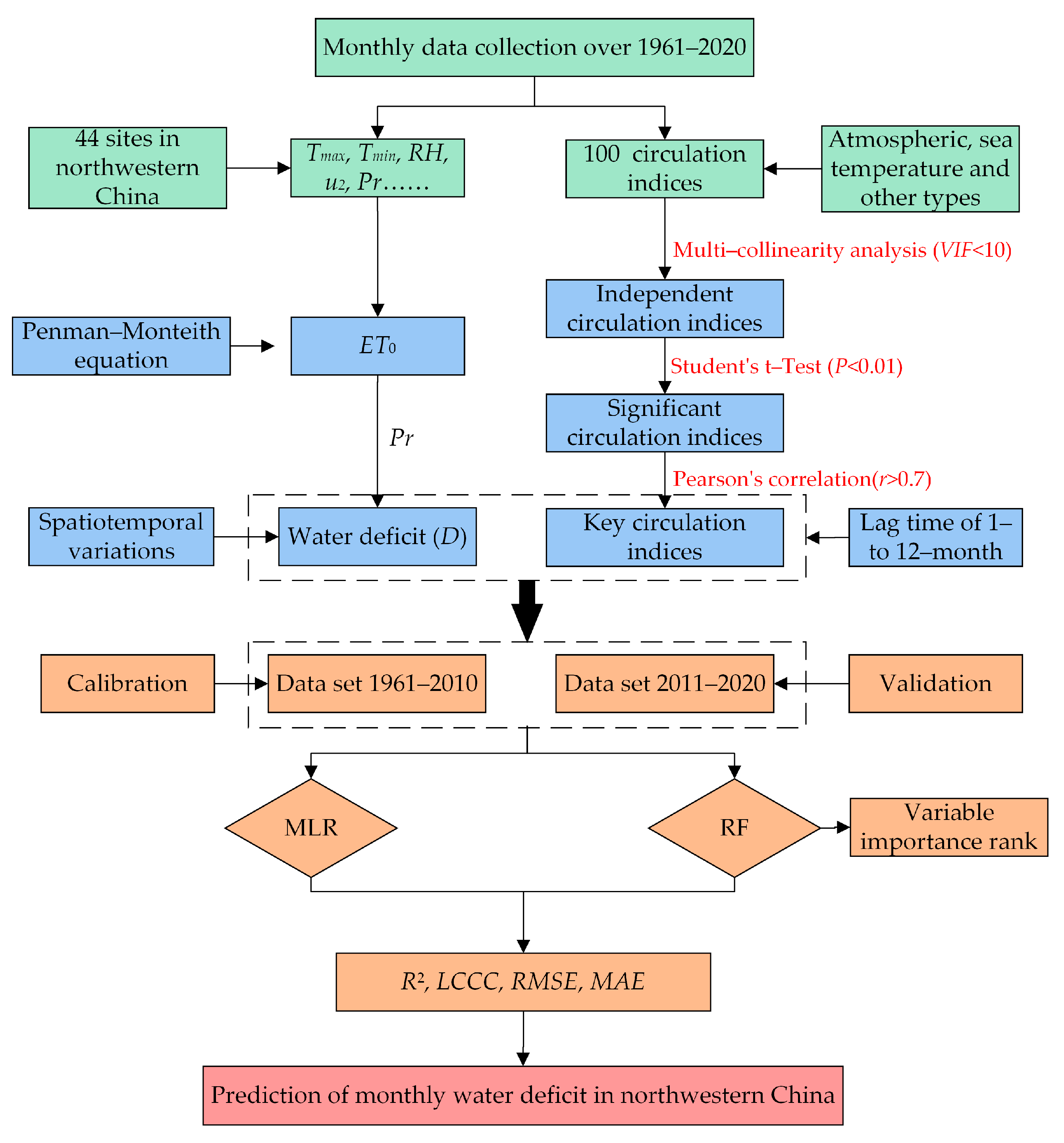
2. Data and Methodology

2.1. Data Collection

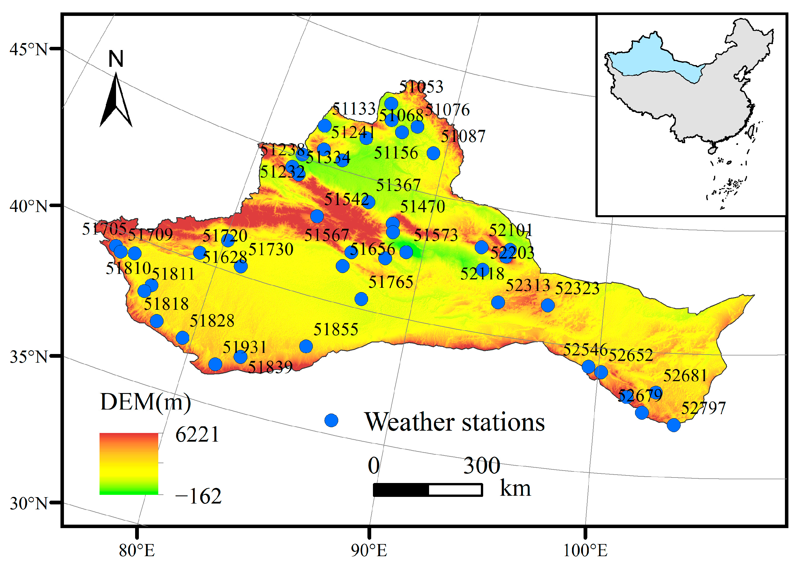
2.1.1. Study Area and Weather Data

The northwestern China is located in inland of the Eurasian continent with an area of approximately 1.91 × 10⁶ km2. This is a transition zone where the west wind belt, the plateau monsoon climate and the East Asian monsoon climate interact. It is an arid and semi-arid region with a typical arid continental climate. The precipitation and temperature in the whole year and winter had a rising trend [24]. Due to the arid climate, the daily and annual temperature ranges are both very large.
The observed daily weather data from 52 national meteorological sites covering 1961−2020 were collected from the China Meteorological Data Service Centre (http://data.cma.cn (accessed on 22 July 2021)). To ensure the consistency and completeness of meteorological data, data with a missing ratio > 1% were deleted. Accordingly, a subset containing 44 sites was used (Figure 1). Missing data were filled using the average data from adjacent 10 sites of the same period [25]. The climate variables include daily minimum and maximum air temperatures, relative humidity, sunshine duration, and wind speed. The data quality and reliability were cross-examined using nonparametric tests including the Kendall autocorrelation test and Mann–Whitney homogeneity tests [26].

2.1.2. The Circulation Indices Data

The 130 monthly circulation indices over 1961−2020 were collected from the National Climate Center of China Meteorological Administration (http://cmdp.ncc-cma.net/cn/download.htm (accessed on 22 July 2021)). There are three types of circulation indices including atmosphere, sea-temperature, and other types. To ensure the data continuity and quality, the circulation index with a missing rate of one month was linearly interpolated using the average value of circulation index in the adjacent 2 months [21], and the circulation index that missed two consecutive months was interpolated using the average value of the current month over the rest of the years of the study period. Regarding the instance where the circulation index that missed three consecutive months or longer was seriously missing, and we excluded it. Finally, 100 circulation indices were retained. Detailed information (namely, the full name, the simplified name, and the classification) of the 100 circulation indices are presented in Table S1.

2.2. Methodology

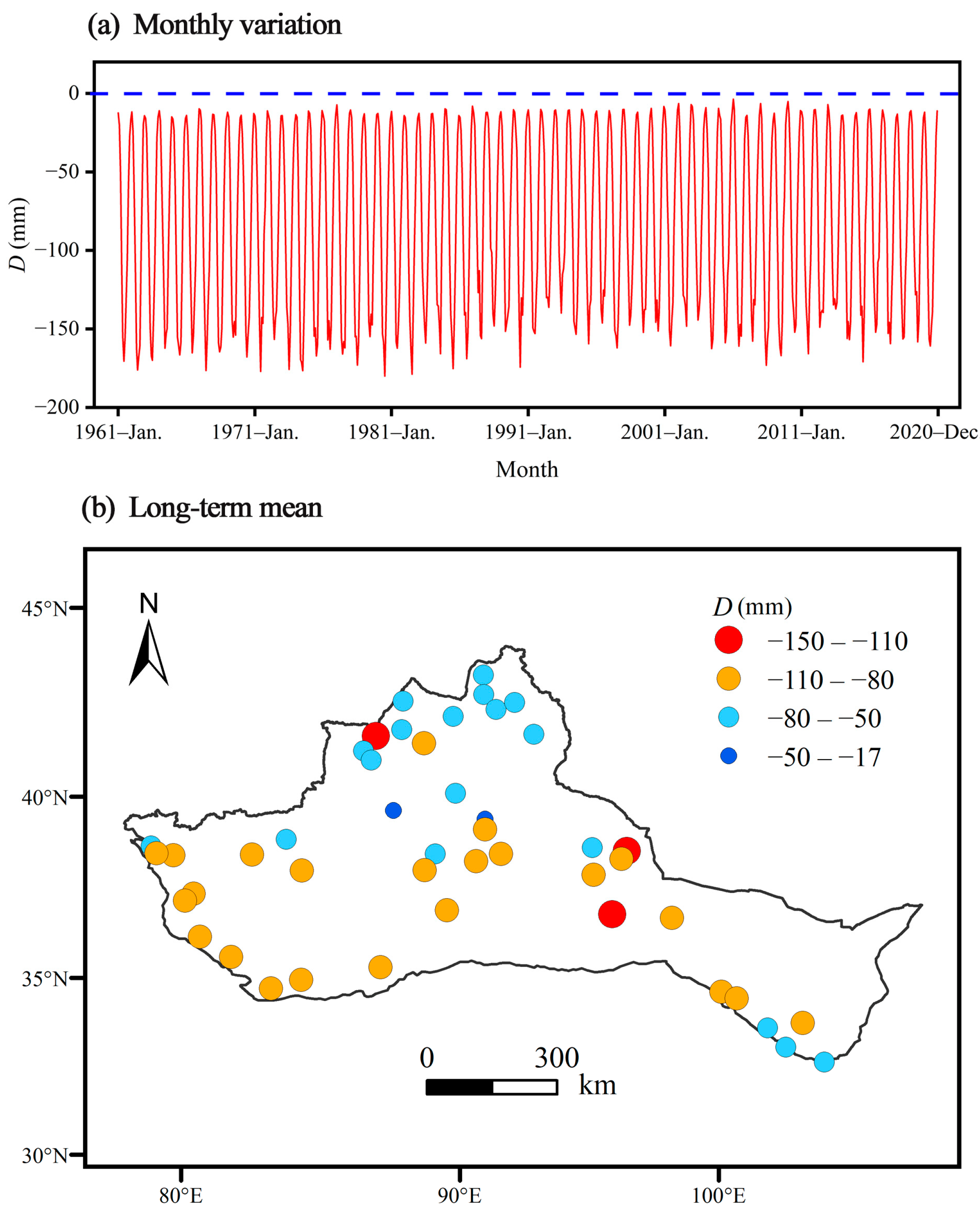
2.2.1. Variation of Water Deficit

Water deficit was calculated on the basis of the difference between precipitation (Pr) and reference crop evapotranspiration (ET0). The D was used to describe the characteristics of water deficit, and the time series of monthly D over 1961−2020 were computed for the selected 44 sites. For computing D, ET0 should be calculated first on the basis of the principle of energy balance and aerodynamics. The Food and Agriculture Organization (FAO) 56 Penman–Monteith equation was applied here for computing ET0 because this equation was developed with theoretical basis and has been proved to have high accuracy around the world [27]. The equation is written as follows:
E T 0 = 0.408 Δ ( R n G ) + γ 900 T + 273 u 2 ( e s e a ) Δ + γ ( 1 + 0.34 u 2 )
where Rn is the net radiation (MJ m−2 day−1); G is the downward ground heat flux (MJ m−2 day−1); Δ is the slope of saturated vapor pressure (kPa °C−1); γ is the psychrometric constant (kPa °C−1); T is the mean air temperature at 2 m (°C); u2 is the winds at 2 m (m s−1); es and ea are saturated and actual vapor pressures, respectively (kPa). Monthly G is estimated by
G = 0.14 ( T k T k 1 )
where Tk and Tk−1 are the average are temperature in the kth and k−1th months, respectively.
Rn is calculated by
R n = R n s R n l
R n s = 0.77 R s
R s = [ 0.25 + 0.75 n N ] R a
R n l = 4.903 × 10 9 ( T max 4 T min 4 4 ) ( 0.34 0.14 e a ) ( 1.35 R s R s o )
where Rns, Rnl, Rs, Ra, and Rso are net shortwave, net longwave, solar, extraterrestrial, and clear sky radiations (MJ m−2 month−1), respectively; n and N are actual and maximum possible sunshine durations, respectively (h); and Tmax and Tmin are maximum and minimum temperatures, respectively.
The parameters es and ea are calculated by
e s = e 0 ( T max ) + e 0 ( T min ) n
e 0 ( T ) = 0.6108 exp ( 17.27 T T + 237.3 )
e a = e 0 ( T min ) × R H max 100
where RHmax is maximum relative humidity (%).
Then, the difference between Pr and ET0 at the ith month, namely, D is obtained by
D i = P r i E T 0 , i
where Di represents water deficit at the ith month.
The temporal variation in data is determined using OriginPro 2023 software, and the maps of the study area and the distribution of sites were mapped using ArcGIS 10.2 software.

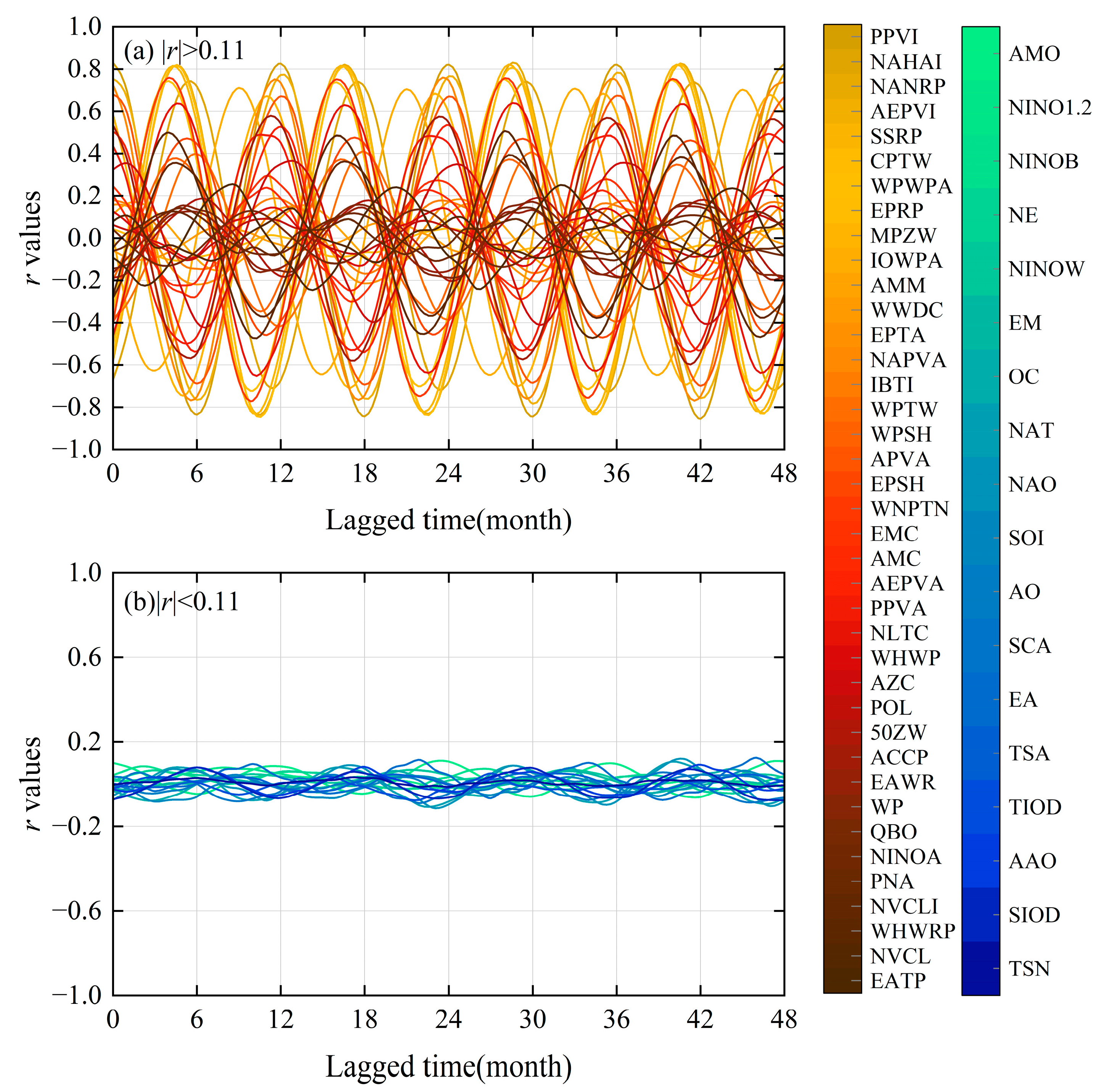
2.2.2. Selection of the Key Circulation Indices

Preliminary Selection of the Independent Circulation Indices

Before conducting the quantitative statistical analysis between circulation indices and D series, it was necessary to conduct multi-collinearity analysis [28] to remove some mutually dependent indices during the regression process. To detect whether there is any collinearity among the 100 circulation indices, the variance inflation factor (VIF) was computed:
V I F j = 1 1 R j 2
where VIFj is variance inflation factor of the jth circulation index, and Rj2 is the coefficient of determination between the jth circulation index and the others.
The threshold of VIFj ≥ 10 was used to infer statistical evidence of significant collinearity [29]. If the jth variable was accounted by at least 90% variance (R2 ≥ 0.9, namely, VIFj ≥ 10) with the other circulation indices, this index has statistically significant collinearity with other variables, and hence it should not be necessarily included in the regression analysis [30]. The test procedure was repeatedly run for several times until VIFj < 10. On the basis of the multi-collinearity analysis, relatively independent monthly circulation indices over 1961–2020 were preliminary retained.

Selection of the Key Circulation Indices

Pearson’s correlation analysis was widely used to show the correlation degree between two time series [31]. Pearson’s correlation coefficient r was performed between monthly D and circulation indices with lag time from 0 to 48 months. The index r ranges from −1 to 1. r > 0 (<0) indicates a positive (negative) correlation; r = 0 indicates no linear relationship. When |r| is close to 1, a higher correlation is implied.
Student’s t test was used to examine whether the monthly D is significantly correlated with the selected circulation indices at the significance level of p < 0.01. However, using enormous circulation indices to predict D would result in a large data set, which is prone to the “curse of dimensionality” and may overfit the model [32,33]. Thus, a strong relation between circulation indices and monthly D with r value of 0.7 was considered to screen the circulation indices for the third time at each climate site [34].

2.2.3. The Quantitative Relationship between D and the Key Circulation Indices

Multi-Variable Linear Regression Model

The multi-variable linear regression (MLR) model was used to establish the quantitative relationship between monthly D (response variable) and the selected key circulation indices (predictor variable) [35]. The largest r value between monthly D and the key circulation indices had certain lagged times (months), at which the key circulation indices were set as the predictor variables sequence. The MLR model is written as
D = a 1 x 1 , l + a 2 x 2 , l + a j x j , l + + a m x m , l + b
where xj is the jth circulation index (j = 1, 2, …, m, m varies with different sites), and aj and b are the fitted coefficients. l represents the lagged months.
For the MLR model, considering the r value between the key circulation index and monthly D had different lagged months, the key circulation indices at the corresponding lagged months (with the maximum r value) were set as the predictor variables sequence. The MLR model was implemented on the basis of the “lm” function in R version 4.1.1.

Random Forest Model

Random forest (RF) is a widely used machine learning decision tree model [36]. Unlike other machine learning methods, RF only needs to adjust two parameters in model training: (i) the number of decision trees growing in the forest (ntree), ntree is 500 by default; (ii) the number of randomly selected features on each node (mtry), mtry is set to one-third of the number of all predictor variables for regression model [13].
Moreover, RF can provide the importance score of each variable during model training process. The importance of the variable is based on the out-of-bag (OOB) regression prediction error. For a training set, RF performs a bootstrap sample and randomly selects g samples for training, then the probability of each sample not being selected is pro = (1 − 1/g)^g. When g becomes larger, pro tends to 1/3, that is, 1/3 of the data are not used in the process of forest formation. Then, this 1/3 of the data are used to evaluate the performance of the RF model [36]. The importance of the variable was computed as a function of the change prediction error by arranging each input variable expressed by the average rate of decrease in accuracy (mean square error). The mean square error (MSEOOB) is calculated by
M S E O O B = 1 n k = 1 n ( O k D O O B , k ) 2
where n is the number of observations, and DOOB,k is the average of all OOB predictions across all trees.
The RF model was implemented using the “randomForest” package of R version 4.1.1. The relative importance of variables is estimated using the “importance” function in the “randomForest” package. All input variables were the same in order to compare the performance of the RF and MLR models for predicting D. The total dataset was divided into the calibration period of 1961–2010 and validation period of 2011−2020 for both MLR and RF models.
For each site in northwestern China, the RF model was to output an importance ranking of predictor variables. Considering the number of total predictor variables and their importance rank change with specific sites, an overall rank in the northwestern China index was proposed to indicate the importance of the selected circulation indices, written as
R a n k i d , N W = i i = 1 44 ( S I i i + 1 R a n k i d , i i ) 2 × I m p i d , i i 44 × S I max
where Rankid,NW is the rank of the idth circulation index in northwestern China; SIii denotes total number of the selected key circulation indices at the iith sites; SImax is the maximal number of the selected circulation indices in northwestern China; Rankid,ii is the rank of the idth circulation index among total SIii circulation indices; Impid,ii is the importance value of the idth circulation index at the iith site (%). Rankid,NW potentially counts the occurrence times (frequency) of the idth circulation index in the studied area and measures its overall importance. The larger the Rankid,NW value, the more important the idth circulation index.

Model Performance Assessment

The performance of the MLR and RF models was assessed using the following four statistical indicators: (i) the coefficient of determination (R2), which reflected the proportion of the response variable explained by the predictor variable through the model; (ii) Lin’s Concordance Correlation Coefficient (LCCC), which assessed the level of agreement between predicted and observed values following the 45° line; (iii) the mean absolute percentage error (MAPE), which measured the percentage error of deviation relative to the observed value; and (iv) the root mean square error (RMSE), which reflected the overall accuracy of the forecast. The equations for computing R2, LCCC, RMSE, and MAPE are referred to in the work of Feng et al. [37].

2.2.4. Prediction of Water Deficit Conditions

The established water deficit models were compared, and the better one was used to predict the water deficit at the 44 sites in northwestern China.
The overall research frame of this research is illustrated in Figure 2.

3. Results

3.1. Spatiotemporal Variations of Month D

The spatiotemporal variations of monthly D over 1961−2020 in northwestern China are shown in Figure 3. First, monthly D in northwestern China over 1961−2020 fluctuated periodically and ranged from −3.7 to −179.9 mm (Figure 3a), and the displayed general water shortage status indicated a severe drought situation in northwestern China. The relatively dry months were June and July, and the relatively wet months were January and December. Second, the spatial distribution of long-term mean monthly D in northwestern China had regional characteristics (Figure 3b). The mean monthly D of the 44 sites in northwestern China ranged from −17.8 to −143.0 mm. We observed higher D values in the southwest, indicating drier conditions in the western south part. Overall, northwestern China was in a state of water deficit.

3.2. Relationship between Monthly D and Circulation Indices

To show the detailed screening process of 100 circulation indices, we chose a sample site (no. 52118, namely, Yiwu site) as an example to select the circulation index that was finally used for modeling.

3.2.1. Preliminary Selected Circulation Indices Considering Multi-Collinearity

On the basis of the rigorous multi-collinearity analysis between monthly D and 100 circulation indices, 57 out of 100 circulation indices with VIF < 10 were finally selected, which was consistent for all of the 44 selected sites (Table 1). The other 43 indices were removed since they had high multi-collinearity.

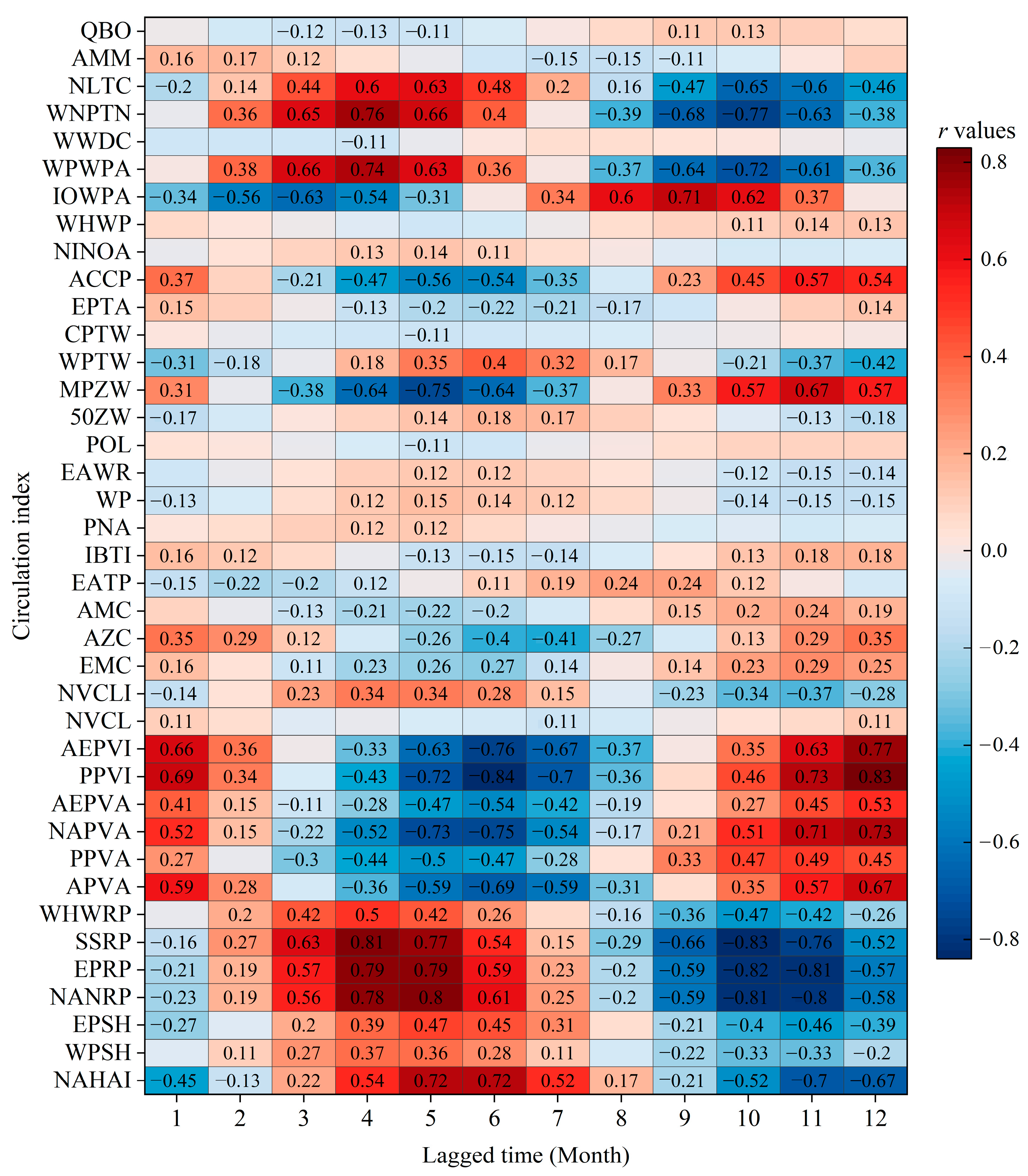
3.2.2. Screen of the Key Circulation Indices

Pearson’s correlation analysis combining Student’s t-test (p < 0.01) were used to screen the key circulation indices that were highly correlated to D series. During this process, the correlations varied with lagged months were necessarily considered.
The r values between monthly D vs. the 57 initially selected circulation indices that lagged from 0 to 48 months were obtained site-specifically. Variations had common features for different sites, and the results for the site no. 52118 was taken as an example (Figure 4). We found the following to be the case: (1) The fluctuations of the r values had a period of 12 months, and monthly D were correlated with circulation indices with the lagged time of 1 to 12 months. The lagged time varied for different circulation indices. (2) Figure 4a,b illustrate the curves of |r| > 0.11 and <0.11, respectively. The water deficit at site no. 52118 were affected by different circulations. The r values were different when the lag time differed (Figure 4a). When the lag time was 6 months and 12 months, the r value between monthly D and PPVI reached −0.84 and 0.83, respectively. (3) There were insignificant correlations between D and 18 circulation indices with −0.11 < r < 0.11 (Figure 4b), and therefore those circulations were screened out from the 57 indices. The remaining 39 circulation indices were meaningful and were maintained for further quantitative analysis of monthly D.
Generally, results for other sites were similar to site no. 52118 in variation patterns of r values. However, different ranks of circulation indices were found for specific sites, which would not be described in detail here.
We considered the period (the largest lag time of water deficit behind circulations) of the r curves was 12 months, at the 0.01 significance level, and then we screened the 39 circulation indices with significance at site no. 52118. The r values between monthly D and the specific circulation index (from the screened 39 ones) varied with changing lag time is demonstrated in Figure 5. The results showed the following: (1) The correlation between monthly D and circulation indices of PPVI, SSRP, EPRP, and NANRP were generally high. At certain lagged time, the circulation index that had the strongest correlations with D changed. For example, when the lag time was 12 months, the r reached the largest (0.83 for D vs. PPVI) and smallest (−0.67 for D vs. NAHAI) levels. Conversely, r reached the largest (0.72 for D vs. NAHAI) and the smallest (−0.84 for D vs. PPVI) levels at the lag time of 6 months. At the 4-month lag time, the r was the largest (0.81 for D vs. SSRP) and the smallest (−0.64 for D vs. MPZW). We suspect that there was a complicated teleconnection relationship between D and specific circulation indices. The reason may be that northwestern China is a transitional zone with an interaction of the westerlies, a plateau monsoon climate, and an east Asian monsoon climate. Moreover, this region has complex terrain, geography, and geomorphology and is very sensitive to climate change and circulations [38] (2) The correlations between D and the nine circulation indices (QBO, WWDC, WHWP, NINOA, CPTW, POL, PNA, WP, NVCL) were relatively poor, with a maximum |r| < 0.14. (3) The number of atmospheric-type circulation indices that were significantly correlated to D was larger than that of sea-temperature-type and other-type circulation indices. For example, when the lagged times were 5, 6, and 12 months, 28, 26, and 26 atmospheric-type circulation indices were significantly correlated with D series, respectively.
Most likely, geographic locations of the study area created the more important impacts of atmospheric-type circulation and less roles of sea-type circulations on monthly D. Northwestern China is located in the highest terrace of the country and far from the sea. In its northwestern part (Xinjiang), there was typical topography of two basins between three mountains. The sea-temperature-type circulations played less important roles in affecting water deficit or climate in northwestern China.
We chose |r| > 0.7 to indicate a strong correlation between the D and circulation indices. The 11 key circulation indices (namely, PPVI, IOWPA, PPVA, AEPVI, SSRP, MPZW, WNPTN, NAHAI, NANRP, WPWPA, and EPRP) were finally selected in site no. 52118.
The finally selected key circulation indices were specific for different sites, and the results are not shown in detail here.

3.3. Quantitative Relationship between Monthly D and the Key Circulation Indices

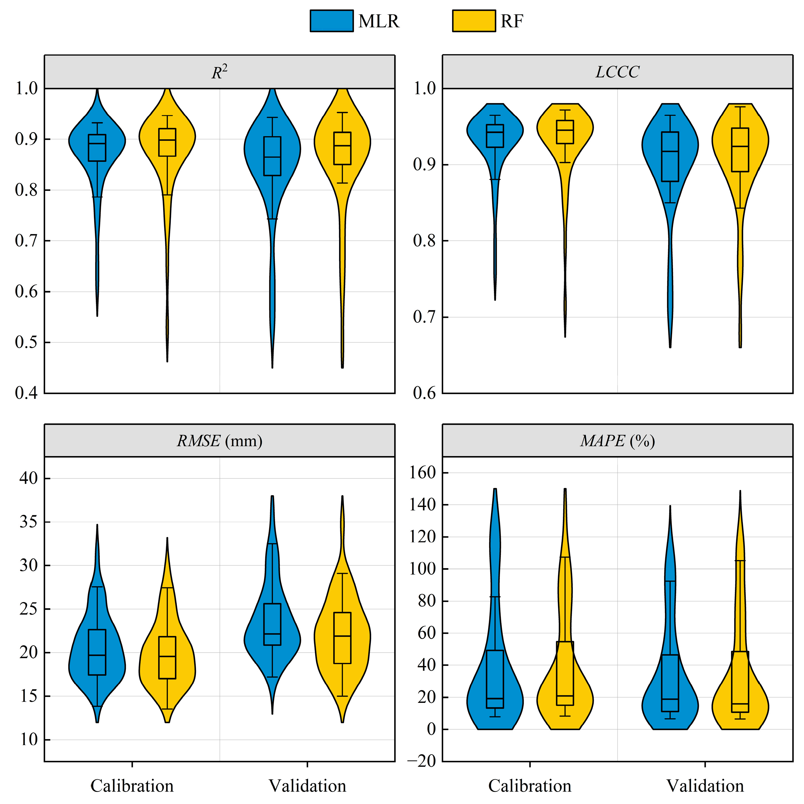
3.3.1. Model Performance Assessment

The performance of MLR- and RF-based models for site-specific D using four statistical indicators (R2, LCCC, RMSE, and MAPE) during the calibration and validation processes are shown in Figure 6. We found the following: (1) In general, both MLR- and RF-based models performed well, with high R2 and LCCC and low RMSE and MAPE values. The ranges of R2, LCCC, RMSE, and MAPE values were 0.488–0.953, 0.677–0.976, 13.5–36.4 mm, and 8.3–158.1%, respectively (MAPE < 50% at 30 sites). According to the R2 values, in the MLR- and RF-based models, the final selected circulation indices explained more than 80% of water deficit conditions at 36 and 38 sites, respectively (Tables S2 and S3). (2) The RF-based model performed better than the MLR-based model, with higher R2 and LCCC and lower RMSE and MAPE values both during the calibration and validation processes. This may be because the RF model considered the nonlinearity between the predictor and response variables. (3) The ranges of R2 and LCCC during the calibration process were higher but lower for RMSE and MAPE than the validation process, which were both found for the MLR and RF models. This was reasonable because data for calibration were greater.
The established MLR equations of monthly D at the nine representative sites are presented in Table 2. Overall, both MLR and RF have satisfactory predictive performance. RF had better predictive effect than MLR because the RF model considered the nonlinear relationship between variables. The model verified the applicability of the MLR and RF models between monthly D and large-scale circulation factors.
We wanted to further demonstrate the performance of MLR and RF models. Therefore, we compared the temporal variations of the MLR- and RF-predicted monthly D with that of the observed values during validation period at the nine representative sites that were distributed in different locations of northwestern China (Figure 7). Both MLR and RF captured the main variation patterns, and their monthly D variations did not deviate from the observed monthly D greatly and showed high consistency at the nine sites. In addition, both essentially captured the peak values very well, but the prediction of the MLR-based model deviated more from the observed D than RF-based model. We think that this result further showed that the performance of RF was better than MLR.

3.3.2. Importance Rank of Predictors

The Impid,ii values (in Equation (6)) of the selected circulation indices (predictors) using RF are provided for the 44 sites in northwestern China in Table 3. The importance rank of the predictor variables at the nine representative sites are illustrated in Figure S1. From the results, the SI changed with specific sites. The SImax was 12 in northwestern China. The Impid,ii differed for all the 44 sites. Taking the Pacific Polar Vortex Strength Index (PPVI) as an example, the index occurred as the largest number at the 23 sites and the second at 10 sites out of 44 sites. PPVI was an important circulation index in denoting water deficit conditions of northwestern China. In addition, the South China Sea Subtropical High Ridge Position Index (SSRP) was an important predictor of the RF prediction models established by the 44 sites in northwestern China.
On the basis of the results shown in Table 3 and Equation 6, we obtained the overall rank of each circulation index in the northwestern China (Table 4), namely, PPVI > SSRP > WPWPA > NANRP > PPVA > IOWPA > AEPVI > WNPTN > NAHAI > MPZW > EPRP > APVA. In particular, PPVI and SSRP had the greatest contributions to the changes in water deficit in northwestern China. The overall ranking created more certainty and was more representative for measuring the importance of the predictors for the studied region with multi-sites.

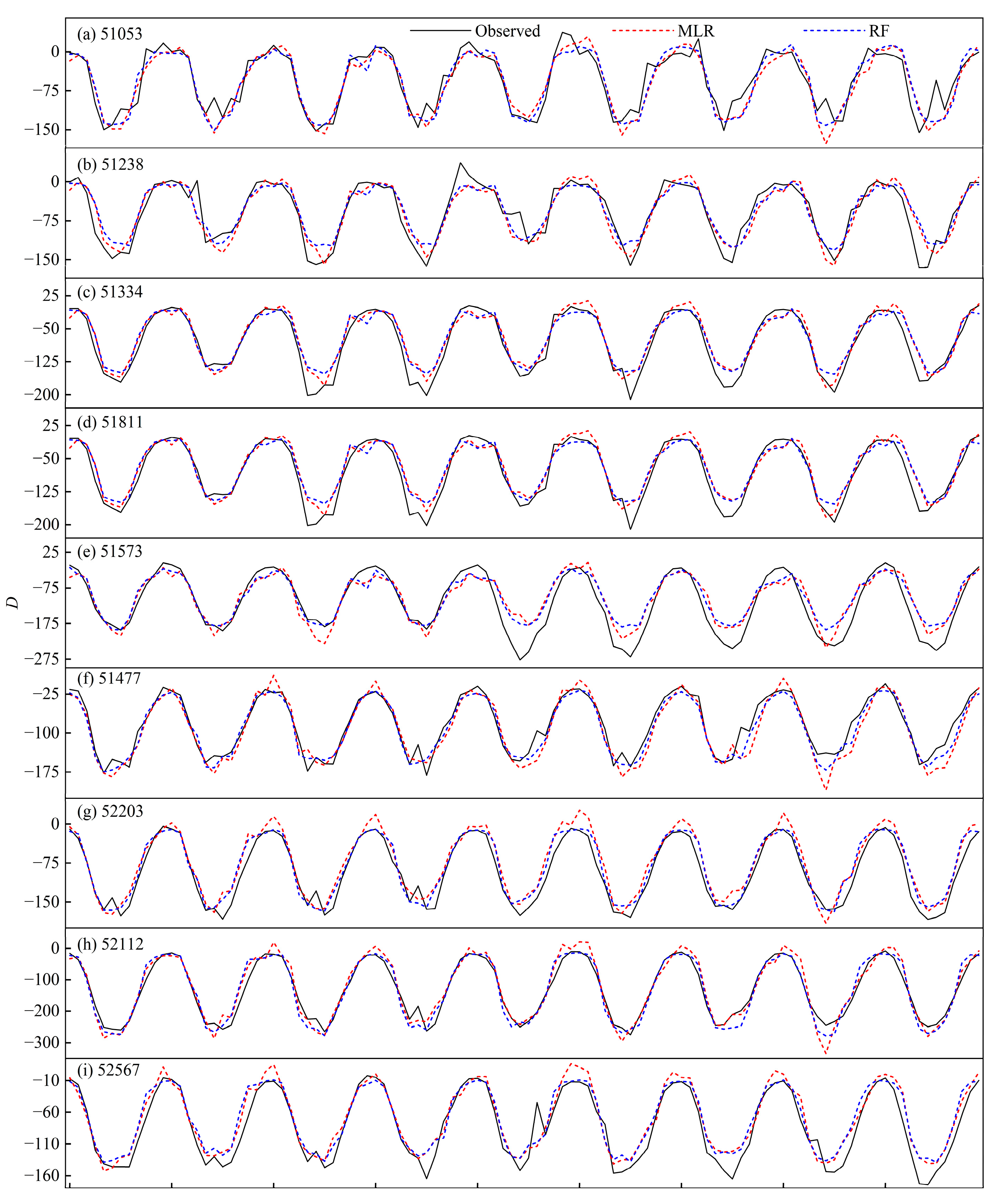
3.4. Forecasted Water Deficit Conditions in Northwestern China

Using the established RF models, we forecasted the monthly D from June 2022 to August 2022 at 44 sites in northwestern China (Figure 8). We found the following: (1) The forecasted D values ranged between −239.7 and −62.3 mm from June 2022 to August 2022. (2) Comparatively, the water deficit conditions in central northwestern China were relatively severe, while the water deficit conditions in western and southeastern northwestern China were less severe. (3) The degree of water deficit was different in northwestern China from June 2022 to August 2022. Overall, the water deficit in northwestern China was the most severe in August 2022, followed by July 2022, and finally June 2022 (Figure 8d).

4. Discussions

4.1. The Necessity of Selecting Key Circulation Indices from over 100 Indices

There were over 100 global large-scale circulation indices available. Selecting main drivers that affect water deficit conditions in northwestern China needs rigorous procedures. Previous research investigated climate drivers determining water deficit conditions. However, the adoption or selection of the predictors was very subjective and without a strict screen procedure. For example, Guo et al. [39] analyzed the correlation between the Multivariate Standardized Reliability and Resilience Index and climate factors (ENSO, AO, and Sunspots) in the upper Yellow River Basin. They found that ENSO and AO had the greatest impact on the evolution of short-term socioeconomic drought in the upper Yellow River Basin, and the impact of ENSO was stronger than that of AO. Irannezhad et al. [40] empirically selected seven circulation indices, namely, AO, NAO, EA, EA/WR, POL, SCA, and WP, to investigate the circulation driving mechanism of the drought in northern Finland over 1962–2011. They found that the development of drought across Finland was most correlated with the EA/WR pattern. Wu et al. [41] calculated r values between Pr/ET0/SPEI and four atmospheric circulation indices (AO, Niño 3.4, PDO, and SST) at the 763 weather sites in China. They found that Pr and ET0 were positively correlated with AO and Niño 3.4 at most sites, while the correlations between Pr/ET0/SPEI and PDO/SST were either positive or negative. Compared with their work, our method considered the impacts of multiple climate drivers including atmosphere, sea temperature, and other types rather than the atmospheric circulation pattern alone.
Former studies were subjective in selecting circulation indices/patterns, which may have overlooked some key circulations and caused uncertainty in forecasting. With the advances of climatology and various climate models, more circulation indices were developed. For example, the circulation indices associated with the Western Pacific Subtropical High system include the Western Pacific Subtropical High Area Index (WPSHA), the Western Pacific Subtropical High Intensity Index (WPSH), the Western Pacific Subtropical High Ridge Position Index (WWRP), the Western Pacific Subtropical High Northern Boundary Position Index (WHNBP), and the Western Pacific Subtropical High West extension ridge point index (WHWRP), among others. Therefore, it was very necessary to screen and determine representative circulation indices for modelling. In our research, we screened the key circulation indices from over 100 indices step by step using several strict procedures and used them to further establish monthly D models with MLR or RF, which both performed well in predicting monthly D.

4.2. Relative Importance of Climate Drivers to Water Deficit

We found that the driven factors of water deficit in northwestern China are mainly related to the circulation events indicated by PPVI, SSRP, WPWPA, NANRP, and PPVA. The importance rank of the circulation indices varied with study sites. We found that PPVI was most important circulation index in determining monthly D in northwestern China. The reason can be summarized as follows: (1) The enhancement of PPVI can bring a great amount of cold air from high latitudes. If water vapor is sufficient, it will lead to more precipitation [42]. (2) PPVI may induce and intensify the activity of the East Asian summer monsoon and affect the precipitation in northern China [43]. (3) The changes of the PPVI are closely related to the interannual fluctuations of precipitation in eastern and western northwestern China, and the PPVI has a significant impact on the climate of northwestern China by affecting AO [44].
Besides PPVI, we found SSRP also plays an important role in affecting water deficit conditions. This result is consistent with previous studies. For example, Chen et al. [45] showed that with the westward movement of the subtropical high in recent decades, a high-pressure center was formed in the eastern part of the Tibetan Plateau. Water vapor from the Indo-Pacific can be transported along the northeastern edge of the Qinghai–Tibet Plateau to northwestern China. Wu et al. [46] pointed out that the rainy season in northwestern China mainly occurring in summer and the change in precipitation are directly related to the weakening of the East Asian summer monsoon accompanied by the westward extension of the subtropical high. These results indicate that SSRP has a potential impact on the water deficit in northwestern China. Notably, heavy rain in Aksu, Xinjiang, on 30 July 2018 caused serious loss of life and property. Due to the compression of the typhoon, the subtropical high moves westward and northward. This circulation pattern has contributed to the infiltration of low-level water vapor in eastern China to Aksu. The westward extension of the subtropical high undoubtedly plays a crucial role in this torrential rain.
Additionally, the WPWPA was ranked as the third most important predictor in our study region. Cai et al. [47] reconstructed hydroclimate of the Inner Mongolia region on the basis of spatial correlation patterns with global sea surface temperature and statistical analysis, and their results showed that the hydroclimate change in Inner Mongolia is closely related to the sea surface temperature of the Indo-Pacific, especially the western Pacific. In addition, our results also showed that the contributions of WNPTN and PPVA to the water deficit in northwestern China were also important, although there were certain spatial differences. This was consistent with previous research that demonstrated that water deficit conditions in various parts of northwestern China were usually the result of multiple climatic driving factors [43,46].

4.3. Prediction of Water Deficit Conditions

Future water deficit conditions can be forecasted in the upcoming months with large-scale climate drivers. Generally, dynamical and statistical methods are used for predicting water deficit (or drought hazards) [48]. The dynamical methods are based on the physical processes of the atmosphere, ocean, and land surface, while statistical methods use different influencing factors as predictors on the basis of empirical relationships from the historical records. Some researchers have projected future droughts at a long-term scale with dynamical methods [49]. However, no single method can adequately describe the overall process of climate system, and there is a large uncertainty in drought prediction using dynamical models in a seasonal scale [48].
By contrast, the statistical methods including traditional regression models and a newly emerged machine learning model have the advantages of low cost and easy application, having been widely used to estimate and forecast water deficit [15,50,51,52] forecasted drought using atmospheric circulation indices with support vector machine (SVM), artificial neural network (ANN), and long short-term memory network in China, and the highest R2 (0.8) was found using their algorithm model. Gao et al. [53] combined circulation (NAO, EA, SCA, POL, etc.) and climate data with ANN to estimate drought in China. Their results showed that the ANN model produced skillful models for most sub-regions (R2max = 0.91). Comparing their results with our work, we had a higher accuracy (R2max = 0.95) of drought forecasting. This may have been because our method considered the impacts of multiple climate drivers. Overall, our study was able to achieve similar or even better performance in forecasting drought than most previous studies.

4.4. Limitations and Future Framework

In this research, we developed a real-time dynamic water deficit forecasting system in northwestern China. We advocate that the forecasting system based on statistical methods should continue to be improved. There are some limitations in our study. Firstly, our work was based on a linear approach to screen key circulation indices, which may affect the accuracy of drought forecasts with selected indicators. In future work, it is likely to adopt some nonlinear methods such as genetic algorithm or BNN to screen key circulation indices and compare their performance with the linear model. Secondly, we derived important circulation patterns (Table 2 and Table 3) that affect the water deficit in northwestern China on the basis of the RF model, but our results lack in-depth exploration of the physical processes in the atmosphere. Future work could consider the development of a hybrid approach using physics-based dynamic models and machine learning techniques to further improve the accuracy of D forecasts. Thirdly, other machine learning techniques such as SVR, BNN, and deep learning can also be used to forecast water deficits in northwestern China. In a recent study, Bibi et al. [54] developed an ensemble-based technique for modeling time series data. The time series data were divided into deterministic and stochastic components and modeled using different techniques, and the final forecasts were obtained by combining the estimates of deterministic and stochastic components. Their research offered a new perspective for the forecasts of D in this paper. Future research should be conducted using more advanced fusion models in order to construct more reliable results in forecasts.

5. Conclusions

We developed a real-time dynamic water deficit forecasting system in northwestern China with a machine learning method using multiple circulation indices and data from 44 observation sites. Our study showed that using machine learning driven by large-scale circulation indices can provide satisfactory water deficit forecasts in northwestern China. We found that RF had a better performance than MLR at all study sites. This may have been due to the fact that the RF model takes into account the nonlinearity between circulation indices and D. We expect that the established RF models can provide a short-term forecast of the dry and wet conditions in northwestern China in the future and provide useful information for monitoring drought/flooding disasters and addressing some disaster prevention caution measures ahead. In addition, we also identified the main predictors of monthly D in northwestern China. PPVI and SSRP were regarded as important predictors in influencing monthly D, which was comparable with results from previous studies. The modelling framework we proposed here will be helpful for the water resource or disaster management department to publicly release some important information to avoid human and economic losses and reduce the risks of nature hazards in northwestern China. The model developed in this study can be easily extended to other sites, regions, and countries around the world.

Supplementary Materials

The following supporting information can be downloaded at: https://www.mdpi.com/article/10.3390/w15061075/s1, Table S1: 100 monthly circulation indices collected from the National Climate Center of China Meteorological Administration. Table S2: Model performance measurements (R2, LCCC, RMSE and MAE) for the calibration period using multi-variable linear regression (MLR) and random forest (RF) at 44 sites in northwestern China. Table S3: Model performance measurements (R2, LCCC, RMSE and MAE) for the validation period using multi-variable linear regression model (MLR) and random forest model (RF) at 44 sites in northwestern China. Figure S1. The importance of different predictor variables used in RF model to predict monthly D at 9 representative sites in northwestern China.

Author Contributions

Conceptualization, Y.L.; data curation, N.Y. and B.N.; formal analysis, L.W.; investigation, P.F.; methodology, K.W., Y.Z. and B.W.; resources, Z.Y.; software, K.W.; validation, K.C. and J.H.; writing—original draft, K.W.; writing—review and editing, Y.L. and G.Y. All authors have read and agreed to the published version of the manuscript.

Funding

This work was supported by the National Natural Science Foundation of China (no. 52079114 and no. 42242003); the Natural Science Foundation of Shenzhen (no. JCYJ20220530161403007); the High-end Foreign Experts Introduction Project (no. G2022172025L); and the Institute of Modern Agricultural Development, SCO Demonstration Base for Agricultural Technology Exchange and Training, Northwest A&F University (no. SCO22A004).

Data Availability Statement

The 44 national weather sites in this research are available from the Meteorological Data Sharing Service Network of China (http://data.cma.cn/ (accessed on 22 July 2021)). The circulation index data used in this research are openly available from the China Meteorology Administration’s National Climate Centre (http://cmdp.ncc-cma.net/cn/index.htm (accessed on 22 July 2021)).

Acknowledgments

The meteorological and circulation data were shared by Service Network in China. Bernie Dominiak and several anonymous reviewers provided us with helpful comments that helped greatly in improving the manuscript.

Conflicts of Interest

The authors declare that they have no known competing financial interests or personal relationships that could have appeared to influence the work reported in this paper.

Abbreviations

AOArtic oscillation
Ddifference of precipitation and ET0
ET0reference crop evapotranspiration
ENSOEl Niño Southern Oscillation
FAOFood and Agriculture Organization
IODIndian Ocean Dipole
IPCCIntergovernmental Panel on Climate Change
LCCCLin’s Concordance Correlation Coefficient
MAPEmean absolute percentage error
MLRmulti-variable linear regression model
NAONorth Atlantic Oscillation
PDOPacific Decade Oscillation
Prprecipitation
R2coefficient of determination
RMSEroot mean square error
RPearson correlation coefficient
SPIstandardized precipitation index
SPEIstandardized precipitation and evapotranspiration index
VIFvariance inflation factor

References

  1. Cook, B.I.; Mankin, J.S.; Anchukaitis, K.J. Climate Change and Drought: From Past to Future. Curr. Clim. Change Rep. 2018, 4, 164–179. [Google Scholar] [CrossRef]
  2. Wei, Y.; Yu, H.P.; Huang, J.P.; Zhou, T.J.; Zhang, M.; Ren, Y. Drylands climate response to transient and stabilized 2 °C and 1.5 °C global warming targets. Clim. Dyn. 2019, 53, 2375–2389. [Google Scholar] [CrossRef]
  3. Kurnik, B.; Kajfež-Bogataj, L.; Horion, S. An assessment of actual evapotranspiration and soil water deficit in agricultural regions in Europe. Int. J. Climatol. 2015, 35, 2451–2471. [Google Scholar] [CrossRef]
  4. Zhao, H.C.; Li, Y.; Chen, X.G.; Wang, H.R.; Yao, N.; Liu, F.G. Monitoring monthly soil moisture conditions in China with temperature vegetation dryness indexes based on an enhanced vegetation index and normalized difference vegetation index. J. Trop. Meteorol. 2021, 143, 159–176. [Google Scholar] [CrossRef]
  5. King, A.D.; Pitman, A.J.; Henley, B.J.; Ukkola, A.M.; Brown, J.R. The role of climate variability in Australian drought. Nat. Clim. Change 2020, 10, 177–179. [Google Scholar] [CrossRef]
  6. Dai, A.; Zhao, T.B.; Chen, J. Climate Change and Drought: A Precipitation and Evaporation Perspective. Curr. Clim. Change Rep. 2018, 4, 301–312. [Google Scholar] [CrossRef]
  7. Vicente-Serrano, S.M.; Beguería, S.; López-Moreno, J.I. A Multiscalar Drought Index Sensitive to Global Warming: The Standardized Precipitation Evapotranspiration Index. J. Clim. 2010, 23, 1696–1718. [Google Scholar] [CrossRef]
  8. Mihăilă, D.; Bistricean, P.I.; Lazurca, L.G.; Briciu, A.E. Climatic water deficit and surplus between the Carpathian Mountains and the Dniester River (1961–2012). Environ. Monit. Assess. 2017, 189, 545. [Google Scholar] [CrossRef] [PubMed]
  9. Das, P.K.; Dutta, D.; Sharma, J.R.; Dadhwal, V.K. Trends and behaviour of meteorological drought (1901–2008) over Indian region using standardized precipitation–evapotranspiration index. Int. J. Climatol. 2016, 36, 909–916. [Google Scholar] [CrossRef]
  10. Somorowska, U. Changes in Drought Conditions in Poland over the Past 60 Years Evaluated by the Standardized Precipitation-Evapotranspiration Index. Acta Geophys. 2016, 64, 2530–2549. [Google Scholar] [CrossRef]
  11. Li, J.; Wang, Z.L.; Wu, X.S.; Xu, C.Y.; Guo, S.L.; Chen, X.H.; Zhang, Z.X. Robust Meteorological Drought Prediction Using Antecedent SST Fluctuations and Machine Learning. Water Resour. Res. 2021, 57, e2020WR029413. [Google Scholar] [CrossRef]
  12. Jiang, S.H.; Wang, M.H.; Ren, L.L.; Xu, C.Y.; Yuan, F.; Liu, Y.; Lu, Y.G.; Shen, H.R. A framework for quantifying the impacts of climate change and human activities on hydrological drought in a semiarid basin of Northern China. Hydrol. Process. 2019, 3, 1075–1088. [Google Scholar] [CrossRef]
  13. Feng, P.Y.; Wang, B.; Luo, J.J.; Liu, D.L.; Waters, C.; Ji, F. Using large-scale climate drivers to forecast meteorological drought condition in growing season across the Australian wheatbelt. Sci. Total Environ. 2020, 724, 138162. [Google Scholar] [CrossRef] [PubMed]
  14. Özger, M.; Mishra, A.K.; Singh, V.P. Low frequency drought variability associated with climate indices. J. Hydrol. 2009, 364, 152–162. [Google Scholar] [CrossRef]
  15. Talaee, P.H.; Tabari, H.; Ardakani, S.S. Hydrological drought in the west of Iran and possible association with large-scale atmospheric circulation patterns. Hydrol. Process. 2014, 28, 764–773. [Google Scholar] [CrossRef]
  16. Manzano, A.; Clemente, M.A.; Morata, A.; Luna, M.Y.; Beguería, S.; Vicente-Serranod, S.M.; Martín, M.L. Analysis of the atmospheric circulation pattern effects over SPEI drought index in Spain. Atmos. Res. 2019, 230, 104630. [Google Scholar] [CrossRef]
  17. Esha, R.I.; Imteaz, M.A. Assessing the predictability of MLR models for long-term streamflow using lagged climate indices as predictors: A case study of NSW (Australia). Hydrol. Res. 2019, 50, 262–281. [Google Scholar] [CrossRef]
  18. Acharya, N.; Singh, A.; Mohanty, U.C.; Nair, A.; Chattopadhyay, S. Performance of general circulation models and their ensembles for the prediction of drought indices over India during summer monsoon. Nat. Hazards 2013, 66, 851–871. [Google Scholar] [CrossRef]
  19. Zhu, X.F.; Hou, C.Y.; Xu, K.; Liu, Y. Establishment of agricultural drought loss models: A comparison of statistical methods. Ecol. Indic. 2020, 112, 106084. [Google Scholar] [CrossRef]
  20. Li, L.C.; Wang, B.; Feng, P.Y.; Wang, H.H.; He, Q.S.; Wang, Y.K.; Liu, D.L.; Li, Y.; He, J.Q.; Feng, H.; et al. Crop yield forecasting and associated optimum lead time analysis based on multi-source environmental data across China. Agric. For. Meteorol. 2021, 308–309, 108558. [Google Scholar] [CrossRef]
  21. Yao, N.; Li, Y.; Lei, T.; Peng, L.L. Drought evolution, severity and trends in mainland China over 1961–2013. Sci. Total Environ. 2018, 616, 73–89. [Google Scholar] [CrossRef]
  22. Ummenhofer, C.C.; D’Arrigo, R.D.; Anchukaitis, K.J.; Buckley, B.M.; Cook, E.R. Links between Indo-Pacific climate variability and drought in the Monsoon Asia Drought Atlas. Clim. Dyn. 2013, 40, 1319–1334. [Google Scholar] [CrossRef]
  23. Xiao, M.; Zhang, Q.; Singh, V.P.; Liu, L. Transitional properties of droughts and related impacts of climate indices in the Pearl River basin, China. J. Hydrol. 2016, 534, 397–406. [Google Scholar] [CrossRef]
  24. Li, B.F.; Chen, Y.N.; Chen, Z.S.; Xiong, H.G.; Lian, L.S. Why does precipitation in northwest China show a significant increasing trend from 1960 to 2010? Atmos. Res. 2016, 167, 275–284. [Google Scholar] [CrossRef]
  25. Yao, N.; Li, Y.; Li, N. Bias correction of precipitation data and its effects on aridity and drought assessment in China over 1961–2015. Sci. Total Environ. 2018, 639, 1015–1027. [Google Scholar] [CrossRef]
  26. Helsel, D.R.; Hirsch, R.M.; Ryberg, K.R.; Archfield, S.A.; Gilroy, E.J. Statistical Methods in Water Resources; Elsevier: Amsterdam, The Netherlands, 1992. [Google Scholar]
  27. Allen, R.G.; Pereira, L.S.; Raes, D.; Smith, M. Crop Evapotranspiration—Guidelines for Computing Crop Water Requirements; FAO Irrigation and Drainage Paper 56; FAO: Rome, Italy, 1998. [Google Scholar]
  28. Stine, R.A. Graphical Interpretation of Variance Inflation Factors. Am. Stat. 1995, 49, 53–56. [Google Scholar] [CrossRef]
  29. Doetterl, S.; Stevens, A.; Six, J.; Merckx, R.; Van Oost, K.; Casanova Pinto, M. Soil carbon storage con-trolled by interactions between geochemistry and climate. Nat. Geosci. 2015, 8, 780–783. [Google Scholar] [CrossRef]
  30. Liu, D.L.; Ji, F.; Wang, B.; Waters, C.; Feng, P.Y.; Darbyshire, R. The implication of spatial interpolated climate data on biophysical modelling in agricultural systems. Int. J. Climatol. 2020, 40, 2870–2890. [Google Scholar] [CrossRef]
  31. Chen, X.G.; Li, Y.; Yao, N.; Liu, D.L.; Javed, T.; Liu, C.C.; Liu, F.G. Impacts of multi-timescale SPEI and SMDI variations on winter wheat yields. Agric. Syst. 2020, 185, 102955. [Google Scholar] [CrossRef]
  32. Wang, B.; Waters, C.; Orgill, S.; Cowie, A.; Clark, A.; Liu, D.L.; Simpson, M.; McGowen, I.; Sides, T. Estimating soil organic carbon stocks using different modelling techniques in the semi-arid rangelands of eastern Australia. Ecol. Indic. 2018, 88, 425–438. [Google Scholar] [CrossRef]
  33. Rodriguez-Galiano, V.; Sanchez-Castillo, M.; Chica-Olmo, M.; Chica-Rivas, M. Machine learning predictive models for mineral prospectivity: An evaluation of neural networks, random forest, regression trees and support vector machines. Ore Geol. Rev. 2015, 71, 804–818. [Google Scholar] [CrossRef]
  34. Eom, Y.S.; Park, B.R.; Shin, H.W.; Kang, D.H. Evaluation of Outdoor Particle Infiltration into Classrooms Considering Air Leakage and Other Building Characteristics in Korean Schools. Sustainability 2021, 13, 7382. [Google Scholar] [CrossRef]
  35. Srisomkiew, S.; Kawahigashi, M.; Limtong, P. Digital mapping of soil chemical properties with limited data in the Thung Kula Ronghai region, Thailand. Geoderma 2021, 389, 114942. [Google Scholar] [CrossRef]
  36. Breiman, L. Random forests. Mach. Learn. 2001, 45, 5–32. [Google Scholar] [CrossRef]
  37. Feng, P.Y.; Wang, B.; Liu, D.L.; Waters, C.; Xiao, D.P.; Shi, L.J.; Yu, Q. Dynamic wheat yield forecasts are improved by a hybrid approach using a biophysical model and machine learning technique. Agric. For. Meteorol. 2021, 285–286, 107922. [Google Scholar] [CrossRef]
  38. Miralles, D.G.; Gentine, P.; Seneviratne, S.I.; Teuling, A.J. Land-atmospheric feedbacks during droughts and heatwaves: State of the science and current challenges. Ann. N. Y. Acad. Sci. 2019, 1436, 19–35. [Google Scholar] [CrossRef]
  39. Guo, Y.; Huang, S.Z.; Huang, Q.; Wang, H.; Fang, W.; Yang, Y.Y.; Wang, L. Assessing socioeconomic drought based on an improved Multivariate Standardized Reliability and Resilience Index. J. Hydrol. 2019, 568, 904–918. [Google Scholar] [CrossRef]
  40. Irannezhad, M.; Ahmadi, B.; Kløve, B.; Moradkhani, H. Atmospheric circulation patterns explaining climatological drought dynamics in the boreal environment of Finland, 1962–2011. Int. J. Climatol. 2017, 37 (Suppl. S1), 801–807. [Google Scholar] [CrossRef]
  41. Wu, M.J.; Li, Y.; Hu, W.; Yao, N.; Li, L.C.; Liu, D.L. Spatiotemporal variability of standardized precipitation evapotranspiration index in mainland China over 1961–2016. Int. J. Climatol. 2020, 40, 4781–4799. [Google Scholar] [CrossRef]
  42. Guan, X.; Yang, L.; Zhang, Y.; Li, J. Spatial distribution, temporal variation, and transport characteristics of atmospheric water vapor over Central Asia and the arid region of China. Glob. Planet. Chang. 2019, 172, 159–178. [Google Scholar] [CrossRef]
  43. Huang, W.; Feng, S.; Chen, J.; Chen, F. Physical mechanisms of summer precipitation variations in the Tarim Basin in northwestern China. J. Clim. 2015, 28, 3579–3591. [Google Scholar] [CrossRef]
  44. Zhang, H.D.; Jin, R.H.; Zhang, Y.S. Relationships between summer northern polar vortex with sub-tropical high and their influence on precipitation in north china. J. Trop. Meteorol. 2008, 24, 417–422. (In Chinese) [Google Scholar]
  45. Chen, C.; Zhang, X.; Lu, H.; Jin, L.; Du, Y.; Chen, F. Increasing summer precipitation in arid central Asia linked to the weakening of the East Asian summer monsoon in the recent decades. Palaeogeogr. Palaeoclimatol. Palaeoecol. 2021, 41, 1024–1038. [Google Scholar] [CrossRef]
  46. Wu, P.; Ding, Y.; Liu, Y.; Li, X. The characteristics of moisture recycling and its impact on regional precipitation against the background of climate warming over Northwest China. Int. J. Climatol. 2019, 39, 5241–5255. [Google Scholar] [CrossRef]
  47. Cai, Q.F.; Liu, Y.; Liu, H.; Ren, J.L. Reconstruction of drought variability in North China and its association with sea surface temperature in the joining area of Asia and Indian–Pacific Ocean. Palaeogeogr. Palaeoclimatol. Palaeoecol. 2015, 417, 554–560. [Google Scholar] [CrossRef]
  48. Yao, N.; Li, Y.; Li, L.C.; Feng, P.Y.; Feng, H.; Liu, D.L.; Liu, Y.; Jiang, K.T.; Hu, X.T.; Li, Y. Projections of drought characteristics in China based on a standardized precipitation and evapotranspiration index and multiple GCMs. Sci. Total Environ. 2020, 704, 135245. [Google Scholar] [CrossRef]
  49. Feng, P.Y.; Wang, B.; Liu, D.L.; Waters, C.; Yu, Q. Incorporating machine learning with biophysical model can improve the evaluation of climate extremes impacts on wheat yield in southeastern Australia. Agric. For. Meteorol. 2019, 275, 100–113. [Google Scholar] [CrossRef]
  50. Forootan, E.; Khaki, M.; Schumacher, M.; Wulfmeyer, V.; Mehrnegar, N.; van Dijke, A.I.J.M. Understanding the global hydrological droughts of 2003–2016 and their relationships with teleconnections. Sci. Total Environ. 2019, 650, 2587–2604. [Google Scholar] [CrossRef] [PubMed]
  51. Hosseini-Moghari, S.M.; Araghinejad, S. Monthly and seasonal drought forecasting using statistical neural networks. Environ. Earth Sci. 2015, 74, 397–412. [Google Scholar] [CrossRef]
  52. Xu, L.; Chen, N.C.; Zhang, X.; Chen, Z.Q. An evaluation of statistical, NMME and hybrid models for drought prediction in China. J. Hydrol. 2018, 566, 235–249. [Google Scholar] [CrossRef]
  53. Gao, Q.G.; Kim, J.S.; Chen, J.; Chen, H.; Lee, J.H. Atmospheric T eleconnection-Based Extreme Drought Prediction in the Core Drought Region in China. Water 2019, 11, 232. [Google Scholar] [CrossRef]
  54. Bibi, N.; Shah, I.; Alsubie, A.; Ali, S.; Lone, S.A. Electricity Spot Prices Forecasting Based on Ensemble Learning. IEEE Access 2021, 9, 150984–150992. [Google Scholar] [CrossRef]
Figure 1. Spatial distribution of weather sites in northwestern China. We used a sample site (no. 52118) located in the central of study area to show in detail the logical process of screening the key circulation indices. DEM is the digital elevation model.
Water 15 01075 g001
Figure 2. The overall framework of the research.
Water 15 01075 g002
Figure 3. The temporal and spatial variation of D in northwestern China.
Water 15 01075 g003
Figure 4. The variations of r values between the monthly D and the selected 57 circulation indices at site no. 52118 when the lagged months ranged from 0 to 48 months.
Water 15 01075 g004
Figure 5. The r values at different lagged times (1–12 months) between monthly D and the specific circulation index (from the selected 39 ones) at the significance level of p < 0.01 for site no. 52118.
Water 15 01075 g005
Figure 6. Results of R2, LCCC, RMSE, and MAPE to show performance of MLR- and RF-based models for site-specific D in northwestern China during the calibration and validation processes. The horizontal line inside the box indicates the median. The box boundary indicates the 25th and 75th percentiles, and the whiskers below and above the box indicate the 10th and 90th percentiles.
Water 15 01075 g006
Figure 7. Comparison of the observed and MLR- and RF-simulated monthly D during the validation period at 9 representative sites in northwestern China.
Water 15 01075 g007
Figure 8. The forecasted monthly D for (a) June 2022, (b) July 2022, and (c) August 2022 based on the established RF models in northwestern China. (d) The violin chart describes the overall situation of D from June to August.
Water 15 01075 g008
Table 1. The initially selected 57 circulation indices from the 100 indices with VIF < 10 through multi-collinearity analysis (consistent at the 44 sites).
Initially Selected Circulation Indices
NAHAIWPSHEPSHNANRPEPRPSSRP
WHWRPAPVAPPVANAPVAAEPVAPPVI
AEPVINVCLNVCLIEMCAZCAMC
EATPIBTIAOAAONAOPNA
EAWPEAWRPOLSCA50ZW
MPZWWPTWCPTWEPTAACCPNINO1 + 2
NINOWNINOANINOBTSAWHWPIOWPA
WPWPAAMOOCWWDCEMNE
TIODSIODWNPTNNLTCTSNSOI
AMMQBONAT
Table 2. The fitted MLR equations between monthly D and the selected key circulation indices of 9 representative sites in northwestern China (the subscript represents the lagged month).
No. of SiteFitted MLR EquationR2LCCCMAPE
(%)
RMSE
(mm)
510530.0088PPVI12 + 0.21NAHAI6 − 1.68SSRP10 − 1.13NANRP11 − 3.32PPVA6 − 0.76MPZW5 + 3.10WPWPA4
− 1.10EPRP11 + 0.0046AEPVI12 − 2.06WNPTN10 − 36.57
0.8630.92744.322.4
51238+0.0071PPVI12−1.41SSRP11 + 3.43WPWPA4 + 4.13
PPVA12 − 0.84NANRP11 + 0.0045AEPVI12 − 0.60MPZW5
− 0.77NAHAI12 − 2.07WNPTN10 − 0.17EPRP11 − 186.38
0.8720.93128.819.0
51334− 0.50NAHAI12 − 1.08NANRP11 − 0.78EPRP11 − 1.34SSRP10
+ 4.55NAPVA12 + 0.0082PPVI12 + 0.0056AEPVI12 − 0.67
MPZW5 + 3.96WPWPA4 − 2.14WNPTN10 − 211.16
0.9190.95811.217.1
51811− 0.0073PPVI6 + 4.78PPVA11 − 0.19SSRP10 − 1.55EPRP11
+ 0.50IOWPA9 + 0.75NAHAI5 + 1.92WPWPA4 − 1.28
NANRP10 + 0.007AEPVI12 − 2.29WNPTN10 − 0.02MPZW5
− 147.04
0.9000.94828.717.5
51573− 2.29SSRP10 + 0.012PPVI12 + 5.70PPVA11 − 0.95WPWPA10
− 1.55NANRP11 + 0.79NAHAI11 − 0.62MPZW5 − 0.92
EPRP11 − 0.09IOWPA3 + 0.0113AEPVI12 − 4.59WNPTN10
− 150.71
0.9030.94927.621.9
51477− 0.0078PPVI6 − 2.30SSRP10 + 2.62NANRP5 − 0.0068
AEPVI6 − 3.98PPVA6 − 0.37IOWPA9 − 1.12EPRP10 + 0.03
NAHAI6 + 1.63WPWPA4 − 2.05WNPTN10 − 0.54MPZW5
+ 10.87
0.8910.94221.321.0
52203− 0.0087PPVI6 + 0.52IOWPA9 − 1.76SSRP10 − 0.0086
AEPVI6 + 0.15NAHAI5 + 2.85WPWPA4 − 2.09APVA6 − 2.51
WNPTN10 − 0.46MPZW5 − 4.56PPVA5 − 1.03NANRP10 − 0.69EPRP10 +88.96
0.9050.95036.719.8
52112− 0.01PPVI6 − 5.51WNPTN10 − 3.32SSRP10 + 0.0169
AEPVI12 − 0.28IOWPA9 + 3.26WPWPA4 − 6.71PPVA6 − 1.61NANRP10 − 0.31APVA6 + 1.13NAHAI5 − 0.59MPZW5
− 0.72EPRP10 + 53.11
0.9300.96419.226.8
51567− 1.96NAPVA5 − 0.0053PPVI6 + 1.75SSRP4 + 0.0092
AEPVI12 + 0.31IOWPA9 − 0.61MPZW5 + 1.48WPWPA4 − 1.21NANRP10 + 0.12NAHAI5 − 1.66APVA6 + 2.66
WNPTN4 − 0.74EPRP10 − 48.82
0.8950.94521.117.4
Table 3. The RF-based rank of the importance for the selected circulation indices at 44 sites in northwestern China.
No. of SitePredictor Variables Importance Ranking (%)
51053PPVI12 (37.1), NAHAI6 (30), SSRP10 (29.3), NANRP11 (29.1), PPVA6 (28.4), MPZW5 (25), WPWPA4 (24.2), EPRP11 (22.1), AEPVI12 (21.7), WNPTN10 (17.5)
51060IOWPA9 (32.5), PPVI12 (32.5), SSRP10 (31.7), NANRP6 (27.4), NAHAI11 (26.9), PPVA6 (26.8), WPWPA4 (24.1), EPRP12 (23.7), AEPVI11 (23), MPZW5 (22.8), WNPTN10 (14.3)
51068PPVI12 (35.5), WPWPA10 (35.2), SSRP4 (33.9), EPRP12 (28.8), NANRP11 (26), PPVA11 (25.6), MPZW5 (23.5), WNPTN12 (22.7), AEPVI10 (21), NAHAI11 (19.9)
51076NAHAI6 (33.5), SSRP10 (32.8), NANRP12 (31.5), AEPVI11 (31.1), PPVI6 (30.9), MPZW5 (29.4), WPWPA4 (26.4), PPVA6 (23.8), EPRP11 (21), WNPTN10 (13.2)
51087PPVA11 (34.2), PPVI12 (33.8), NANRP12 (32.7), SSRP10 (32), MPZW5 (25), EPRP11 (24.8), WPWPA10 (22.4), AEPVI10 (15.9), NAHAI12 (14.1), WNPTN11 (13)
51133PPVI6 (36.5), AEPVI12 (36.4), SSRP11 (33.9), PPVA10 (25.8), WPWPA11 (25.5), NANRP12 (24.6), NAHAI11 (18.8), EPRP12 (18.4), WNPTN10 (12.9)
51156PPVI12 (36.5), SSRP10 (34.4), MPZW5 (32.6), WPWPA10 (30.5), PPVA12 (23.9), NANRP12 (22.8), AEPVI11 (22.4), WNPTN10 (17.7), EPRP11 (15.3)
51232PPVI12 (41.2), WPWPA4 (36.3), NAHAI6 (33.1), SSRP12 (31.7), AEPVI11 (29.2), NANRP11 (27.9), PPVA6 (27.6), MPZW5 (26.2), EPRP11 (21.2), WNPTN10 (16.3)
51238PPVI12 (40.6), SSRP11 (32.2), WPWPA4 (31.6), PPVA12 (27.6), NANRP11 (27.3), AEPVI5 (25.8), MPZW12 (23.9), NAHAI12 (21.2), WNPTN11 (17.2), EPRP10 (16.6)
51241AEPVI6 (43), PPVI12 (36.8), SSRP11 (30.9), NANRP11 (20), EPRP11 (18.9), PPVA12 (18.6), WNPTN10 (11.8)
51243PPVI6 (42.5), IOWPA11 (31.2), NAHAI9 (30.1), NANRP6 (29.8), SSRP10 (25.3), EPRP11 (22.2), PPVA6 (21), AEPVI5 (15.8), WPWPA6 (15.7), MPZW4 (15), WNPTN10 (6.1)
51334PPVI12 (37.8), SSRP10 (36.9), WPWPA4 (34.3), PPVA11 (30.6), NANRP5 (28.3), NAHAI12 (27.8), AEPVI12 (26.9), MPZW12 (26.6), EPRP11 (21.4), WNPTN10 (12.6)
51367WPWPA4 (40.3), SSRP11 (39.4), PPVI12 (36.7), AEPVI12 (31.4), MPZW5 (30.3), NANRP11 (26.3), PPVA12 (24), NAHAI12 (22.1), IOWPA3 (20.2), EPRP11 (15.9), WNPTN10 (14.9)
51477PPVI6 (37.4), SSRP10 (29.1), NANRP6 (28.8), AEPVI5 (25.3), PPVA9 (25.1), IOWPA6 (24.2), EPRP6 (17.6), NAHAI10 (17.4), WPWPA4 (15), WNPTN10 (13.1), MPZW5 (11.1)
51526PPVI4 (34.9), SSRP6 (34.7), PPVA12 (28.7), NANRP9 (28.4), IOWPA5 (25), WPWPA10 (23.2), AEPVI6 (23), NAHAI5 (19.9), EPRP10 (18.8), MPZW6 (17.3), APVA5 (16.7), WNPTN4 (11.6)
51567PPVI6 (37.1), SSRP4 (32), AEPVI12 (31.1), IOWPA9 (29.8), MPZW5 (25), WPWPA4 (24.1), NANRP5 (22.3), NAHAI5 (21.5), APVA10 (20.4), PPVA6 (19.7), WNPTN4 (17.9), EPRP10 (16)
51573SSRP10 (39.5), PPVI12 (36.7), PPVA10 (31.8), WPWPA11 (31.3), NANRP11 (29.5), NAHAI11 (28.2), MPZW3 (26), EPRP11 (24.8), IOWPA5 (24.3), AEPVI10 (24.1), WNPTN12 (21.7)
51628WNPTN4 (37.9), PPVI12 (37.7), SSRP10 (31.5), PPVA11 (30.4), WPWPA10 (27.6), NANRP11 (24.9), MPZW10 (24), EPRP10 (21.9), NAHAI11 (20.7), AEPVI12 (19.3), APVA12 (15)
51656WPWPA4 (36.8), SSRP4 (34.6), PPVI6 (33.6), IOWPA9 (33.1), MPZW5 (28.9), PPVA5 (26), NANRP4 (24.6), WNPTN4 (24.4), NAHAI5 (21.8), APVA6 (21), AEPVI6 (17.7), EPRP4 (17.5)
51704PPVI6 (39.9), NANRP11 (32.2), IOWPA10 (28.9), SSRP9 (28), AEPVI10 (23.8), NAHAI4 (23.4), WNPTN6 (21.6), WPWPA5 (19.6), EPRP11 (18.1), MPZW6 (16.9), PPVA6 (16.5)
51705EPRP11 (37), PPVI10 (35.4), SSRP12 (34.1), WNPTN10 (31.5), AEPVI12 (26.1), NANRP11 (22.2)
51709PPVI12 (37.5), WPWPA11 (36.9), SSRP10 (33.8), PPVA5 (33.6), MPZW10 (30.2), EPRP10 (29.1), WNPTN11 (28.9), NANRP11 (25.2), AEPVI3 (21.9), IOWPA12 (21), NAHAI11 (19.4)
51720PPVI6 (36.3), WPWPA4 (36), NANRP4 (26.4), SSRP9 (26), AEPVI5 (23.9), IOWPA6 (23.7), PPVA6 (23.1), NAHAI10 (21.2), WNPTN5 (20.3), EPRP5 (14.7)
51730PPVI6 (38.2), IOWPA10 (35.8), SSRP9 (28.6), WNPTN10 (27.4), AEPVI4 (23.3), WPWPA6 (23), NAHAI5 (21.7), NANRP10 (20.7), PPVA6 (18.1), MPZW5 (17.8), APVA10 (17.3), EPRP5 (15.5)
51765PPVI6 (38.2), IOWPA9 (32), SSRP4 (31), NANRP4 (29.3), WPWPA10 (28.7), WNPTN4 (24.8), PPVA5 (24.3), MPZW6 (23.6), AEPVI6 (23.1), APVA5 (20.2), NAHAI5 (18.6), EPRP10 (16.8)
51810PPVI6 (43.8), IOWPA4 (38.8), WPWPA11 (31.8), PPVA9 (30.3), SSRP10 (25.9), WNPTN10 (25.7), AEPVI12 (20.6), MPZW5 (18.1), NANRP10 (18), NAHAI11 (17.5), EPRP10 (11.5)
51811PPVI6 (46.9), PPVA9 (28.8), SSRP11 (27.5), EPRP5 (26.8), IOWPA10 (25.8), NAHAI11 (25), WPWPA4 (22.2), NANRP10 (20.1), AEPVI12 (19.5), WNPTN10 (18.9), MPZW5 (14.3)
51818NANRP6 (36.7), PPVI5 (34.1), SSRP4 (31.9), AEPVI12 (27.9), PPVA11 (27.3), NAHAI11 (25.8), MPZW10 (21.2), WPWPA5 (21.1), EPRP10 (16.8), WNPTN4 (13.7)
51828AEPVI5 (33.6), SSRP6 (32.9), PPVI12 (32.6), NANRP4 (32.5), NAHAI11 (27.2), MPZW5 (22.9), PPVA11 (21.9), WPWPA10 (21.1), IOWPA9 (17.2), EPRP12 (15.5), APVA10 (13.7), WNPTN4 (13)
51839AEPVI12 (36.5), PPVI6 (34.3), PPVA11 (33.6), SSRP4 (33.4), NANRP5 (31.6), WPWPA10 (28.2), IOWPA5 (23.1), APVA6 (22), NAHAI10 (20.8), EPRP9 (18.3), WNPTN4 (16), MPZW5 (12.5)
51855WPWPA4 (35.7), SSRP4 (34.1), PPVI6 (31.1), IOWPA9 (29), NANRP5 (26.6), AEPVI6 (25.9), PPVA5 (24.3), EPRP5 (23.8), APVA6 (21.8), NAHAI5 (18.8), MPZW5 (16.8), WNPTN4 (9.8)
51931PPVI5 (35.7), SSRP6 (33.7), NANRP4 (31.6), APVA4 (25.1), AEPVI6 (24.7), WPWPA9 (23.9), IOWPA6 (23.3), PPVA5 (23.3), MPZW10 (22.7), EPRP5 (21.3), NAHAI5 (19.8), WNPTN4 (11.4)
52101WNPTN4 (38.8), PPVI12 (36.6), WPWPA10 (25.3), EPRP10 (23.8), SSRP10 (23.3), PPVA6 (22.5), MPZW10 (17), NANRP5 (16.5), AEPVI12 (14.2)
52112PPVI6 (43.2), WNPTN9 (33.4), SSRP10 (29.5), AEPVI12 (28.8), IOWPA10 (28.5), WPWPA4 (26.7), PPVA6 (26.1), NANRP10 (20.8), APVA5 (20.4), NAHAI6 (15.5), MPZW10 (14.7), EPRP5 (13.7)
52118PPVI6 (45), IOWPA9 (31.6), PPVA10 (28.3), AEPVI6 (25.8), SSRP12 (25.4), MPZW5 (22.9), WNPTN5 (20.9), NAHAI10 (19), NANRP10 (17.1), WPWPA10 (14.7), EPRP4 (13.8)
52203PPVI6 (41.1), IOWPA9 (33.5), SSRP10 (27.8), AEPVI5 (24.9), NAHAI4 (24.2), WPWPA6 (23.7), APVA5 (23.2), WNPTN10 (22.3), MPZW10 (20.2), PPVA6 (20.2), NANRP5 (16.5), EPRP10 (12)
52313EPRP11 (39.2), PPVI6 (38.6), SSRP4 (34.5), NANRP5 (28.1), MPZW10 (21.4), WPWPA6 (21.1), WNPTN10 (20.5), AEPVI6 (20.4), NAHAI6 (19.4), PPVA5 (17.5), APVA6 (14.4)
52323WNPTN4 (48), SSRP10 (33.7), PPVI12 (32.7), MPZW5 (32.7), EPRP11 (28.6), WPWPA10 (26.8), AEPVI11 (24.6), NANRP12 (24.2), NAHAI12 (22.5), APVA12 (20.5), PPVA12 (18.3)
52546PPVI6 (40.5), IOWPA9 (28), NAHAI5 (26.9), WNPTN12 (24.4), AEPVI11 (23.4), SSRP4 (23.3), PPVA10 (22.8), NANRP10 (20.5), MPZW5 (17.3), WPWPA10 (16.8), EPRP4 (16.3)
52652WNPTN4 (48.1), PPVA11 (31.9), SSRP10 (29.2), PPVI12 (28.6), AEPVI10 (27), MPZW5 (25.4), EPRP12 (24.8), WPWPA10 (23.1), NANRP10 (22.7), NAHAI11 (10.7)
52674EPRP10 (55.5), NANRP10 (49.2)
52679EPRP10 (31.7), PPVA11 (31.2), SSRP10 (28.6), NANRP10 (25.9), NAHAI11 (19.9), AEPVI12 (15.7), PPVI11 (14.9)
52681PPVA11 (33.6), WPWPA12 (31.3), APVA10 (29.1), PPVI10 (28.6), NANRP12 (28), SSRP10 (26.4), EPRP10 (25.2), WNPTN10 (22.5), NAHAI5 (18.6), MPZW11 (16.3), AEPVI12 (15.7)
52797SSRP10 (42.2), EPRP10 (35.4), NANRP10 (31.9), PPVI11 (27.2)
Table 4. The overall importance rank of 12 circulation indexes in northwestern China.
Circulation IndexPPVISSRPWPWPANANRPPPVAIOWPAAEPVIWNPTNNAHAIMPZWEPRPAPVA
Rankid,NW2.9591.9281.1350.9620.9410.9000.8560.6310.5070.4060.4010.141
Disclaimer/Publisher’s Note: The statements, opinions and data contained in all publications are solely those of the individual author(s) and contributor(s) and not of MDPI and/or the editor(s). MDPI and/or the editor(s) disclaim responsibility for any injury to people or property resulting from any ideas, methods, instructions or products referred to in the content.

