The Significance of Groundwater Table Inclination for Nature-Based Replenishment of Groundwater-Dependent Ecosystems by Managed Aquifer Recharge

Abstract

Managed aquifer recharge (MAR) is an increasingly popular technique; however, the significance of groundwater flow dynamics is rarely examined in detail regarding MAR systems. In general, a high hydraulic gradient is not favoured for MAR implementation, as it causes higher water loss and mixing of recharge water with native groundwater. However, during groundwater-dependent ecosystem (GDE) rehabilitation, these hydraulic gradient-driven flow processes can be taken advantage of. The aim of this research is to test this hypothesis by evaluating the effect of groundwater table inclination, topography, and other local characteristics on MAR efficiency from the perspective of GDE restoration. MAR efficiency was examined from recharge to discharge area in a simple half-basin based on theoretical flow simulations, using GeoStudio SEEP/W software. Different scenarios were compared to analyse the groundwater level increase and the infiltrated water volumes and to assess the efficiency of MAR based on these parameters in each scenario. The theoretical results were applied to a close-to-real situation of Lake Kondor, a GDE of the Danube-Tisza Interfluve (Hungary), which dried up in the past decades due to groundwater decline in the area. Based on the results, initial hydraulic head difference, model length, and hydraulic conductivity are the most critical parameters regarding water level increase at the discharge area. The water amount needed for increasing the water table is mainly influenced by the thickness of the unsaturated zone and the material properties of the aquifer. The findings can help better understand MAR efficiency in light of local groundwater flow processes and contribute to optimising MAR systems. The results of the study suggest that, if water is infiltrated at the local recharge area, the water table will also increase at the corresponding discharge area, which positively effects the connected GDEs. This approach can serve as a nature-based solution (NBS) to sustain sensitive ecosystems in changing climatic conditions.

1. Introduction

Managed aquifer recharge (MAR) is a group of diverse methods to purposefully recharge groundwater for subsequent recovery or environmental benefits [1]. It has numerous positive effects on the environment, as it helps improve water quantity and quality, build underground water storage, sustain groundwater-dependent ecosystems (GDEs), reduce land subsidence, etc. [2,3,4,5,6].

In certain cases, the main aim of MAR implementation is not specifically or exclusively water retention and later abstraction, but the rehabilitation of groundwater reserves and groundwater-dependent ecosystems [7,8,9]. Instead of working against nature (as a general practice), if natural processes are understood and proactively utilised, solutions mimicking nature could form a base for future improved management of natural resources. These nature-based solutions can enhance natural groundwater recharge only if the natural groundwater flow characteristics are considered. In this regard, MAR can be used to enhance natural recharge. Therefore, it can be considered as a nature-based solution (NBS) [10,11]. Groundwater and aquifer-related NBS, such as MAR, have the potential to alleviate the impacts of extreme hydroclimatic conditions by managing infiltration and providing ecological benefits for groundwater-dependent ecosystems [11].

Even though the popularity of MAR systems is increasing, and the range of applications is getting broader, including monitoring, risk, impact assessment, and legal and institutional aspects [12,13,14,15,16,17], groundwater flow systems and their regional and local characteristics [18,19], e.g., distribution of natural recharge and discharge areas, as well as groundwater table inclination, are generally not considered in MAR research.

Nevertheless, there are MAR types that take advantage of the sloping terrain, especially those which are aimed at collecting water (e.g., stormwater). These methods include recharge dams, sand dams, subsurface dams, barriers, and bunds [20]. Dune filtration also takes advantage of the hydraulic gradient, where the main aim of water infiltration is water quality improvement. The Aquifer Storage Transfer and Recovery (ASTR) method aims at water purification, as well, for which a low or moderate lateral flow rate can be beneficial [21,22]. In most cases, high hydraulic gradient and high lateral flow rate are considered disadvantageous, as these allow the mixing of recharged water with native groundwater [23,24,25]. It is especially crucial in the case of underground water storage in brackish aquifers [22,26,27].

In MAR-related research, recharge processes, mounding, and attenuation are frequently assessed either from theoretical (e.g., [28,29,30,31,32]) or from practical (e.g., [33,34,35]) points of view. In contrast, the effects and significance of hydraulic gradient and flow dynamics for a simple basin are rarely investigated in detail, although from a modelling perspective, hydraulic gradient is often considered (e.g., [27,36,37,38,39]). Some research focuses on recharge and mounding processes (e.g., [40,41,42]) and others on contaminant attenuation and mixing of injected water with native groundwater (e.g., [27,38,43]). On the other hand, the potential positive effects of groundwater flow have not been systematically investigated before.

In light of recent climate change [44,45] and its cross-sectoral effects (e.g., [46,47]), nature-based solutions and managed aquifer recharge are getting more important to adapt to climate change and increase sustainability [48,49,50]. Recent research proved that climate change has an effect on groundwater flow systems and, consequently, on groundwater-dependent ecosystems, as well (e.g., [51,52,53,54]). Human activities, such as groundwater abstraction, land drainage, canalisation, etc., can have similar impacts by decreasing the water table and altering local flow systems (e.g., [51,55]). Managed aquifer recharge can help mitigate these consequences by reversing these processes (e.g., [56,57]). Although high horizontal hydraulic gradient is often not favoured for MAR implementation, as it causes higher water loss and mixing of recharged water with native groundwater [23,24,58], in the case of GDE rehabilitation, these processes could be taken advantage of.

Based on these theoretical assumptions, the two main aims of this research are the following:

i.

to evaluate the effects of groundwater table inclination and further influencing parameters (topography, model length, groundwater depth, material properties, heterogeneity, and infiltration basin parameters) on downgradient water level increase and to estimate infiltration-based MAR efficiency from the perspective of water level and GDE restoration for a simple half-basin; and

ii.

to demonstrate the applicability of this method through a close-to-real situation, answering the hypothetical question: “Can this be a possible measure to rehabilitate the former Lake Kondor, Danube-Tisza Interfluve, Hungary?”

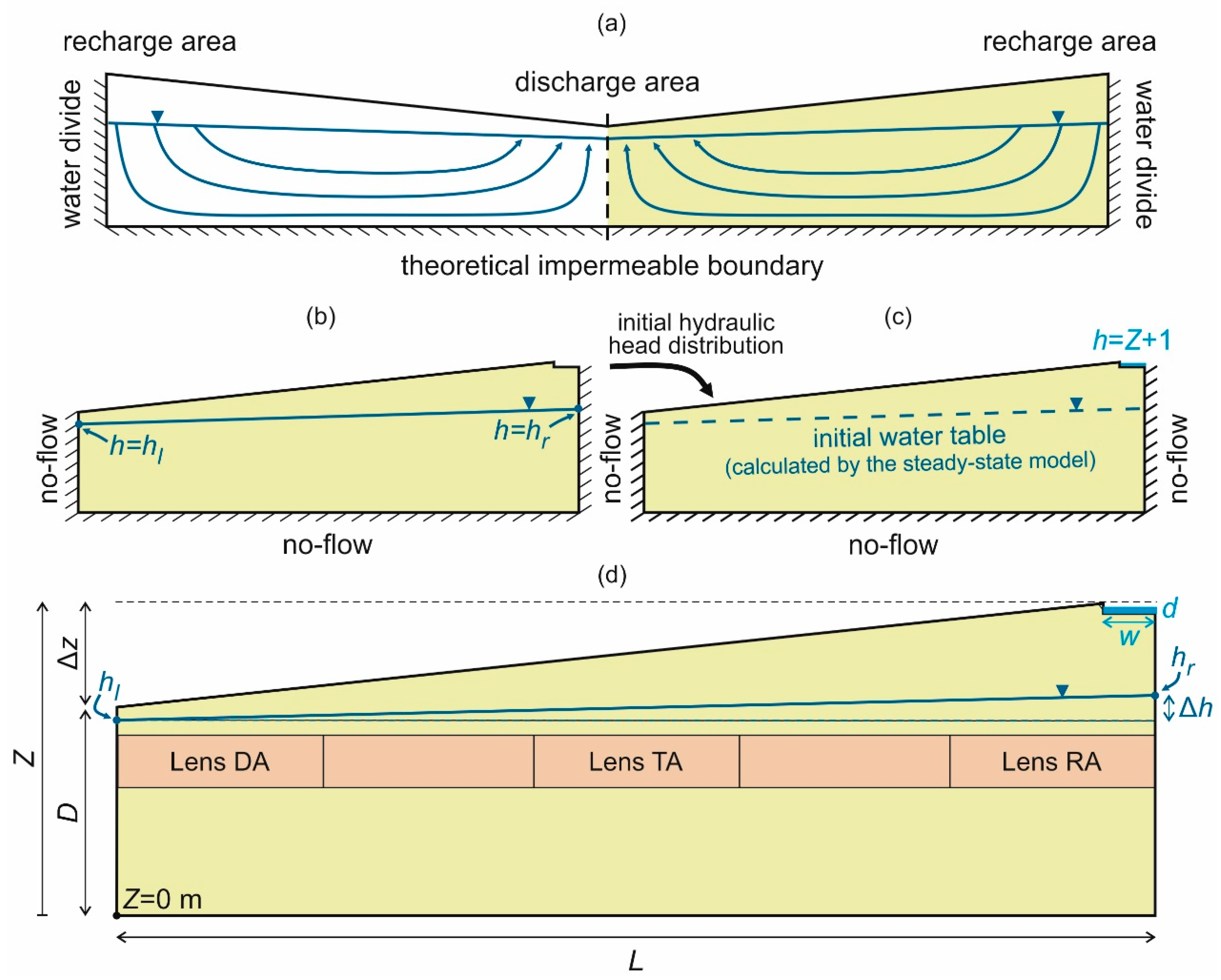
2. Theoretical Models

2.1. Methods

The effects of groundwater table inclination on managed aquifer recharge with an infiltration basin were investigated from recharge to discharge area for a theoretical shallow half-basin [59,60,61,62,63,64] (Figure 1) through theoretical model scenarios.

For comprehensive analysis, two-dimensional saturated–unsaturated numerical flow simulations were carried out using the GeoStudio SEEP/W finite element software, which was designed for modelling variably saturated porous media [65]. The transient flow problem is described by the following differential equation (diffusion equation) Equation (1):

$$\frac{\partial }{\partial x}\left[K{\left(\mathsf{\theta }\right)}_{xx}\frac{\partial h}{\partial x}\right]+\frac{\partial }{\partial z}\left[K{\left(\mathsf{\theta }\right)}_{zz}\frac{\partial h}{\partial z}\right]+Q= m_w{\gamma }_w\frac{\partial h}{\partial t}$$

(1)

where h is the hydraulic head [m], K_xx is the hydraulic conductivity in the x-direction [m/s], K_zz is the hydraulic conductivity in the z-direction [m/s], Q is the applied boundary flux [m³/s], θ is the volumetric water content [-], m_w is the slope of the saturated water content function, γ_w is the water specific weight [kN/m³], and t is the time [s] [65]. The hydraulic conductivity in the saturated zone is constant; however, it is dependent on θ and estimated by the van Genuchten method [66] in the unsaturated zone. Steady-state calculations were performed using a simplified version of Equation (1) (t = 0) to determine the initial conditions for the time-dependent calculations.

The model geometry and the applied boundary conditions (Figure 1b–d) imitate a theoretical half-basin with water divides at the two sides and an impermeable boundary at the bottom. Due to geometrical reasons (symmetry of the whole basin; Figure 1a), the lateral boundaries at the recharge and discharge areas can be approximated with a no-flow boundary [59,60,61,62,63,64], which can be described by the following equation, Equation (2):

$$-n·{\mathsf{\rho }}_{\mathrm{w}}·q=0$$

(2)

where n is the normal vector, ρ_w is the water density, and q denotes the Darcy flux. These boundary conditions were used for both steady-state and time-dependent calculations (Figure 1b,c).

The position of the water table was prescribed by constant heads on the left and right sides of the model (Figure 1b). The initial condition for the time-dependent groundwater flow problem was the pressure or hydraulic head distribution obtained from the stationary solution of Equation (1).

The infiltration basin was only active in the transient models and was specified by constant head-type boundary conditions (Figure 1c), which generated a time-dependent flux (Q) from the basin to the model.

Simplified basins are used in many cases to understand processes operating on the effect of basin-scale groundwater flow on different processes (e.g., [59,60,61,62,63,64]). Adequately, these simple boundary conditions were selected to focus on the groundwater table and its direct effects on managed aquifer recharge and to avoid the interaction of different processes, such as precipitation, evapotranspiration, and lateral flow.

Six main scenario groups (SGs) were implemented, consisting of 295 scenarios in total (see

Table 1. Model scenarios with the studied parameters for the theoretical simulations (1–6) and the case study (7).

Parameters	Units	1. Topography (SG-1)	2. Model Length (SG-2)	3. Elevation of Water Table (SG-3)		4. Material Properties (SG-4)			5. Heterogeneity (SG-5)	6. Basin Parameters (SG-6)		7. Case Study (K1–3)
				A. Discharge Area	B. Recharge Area	A. Kxx	B. ε	C. θs		A. w	B. d
Length (L)	m	2000	2000–10,000	2000	2000	2000	2000	2000	2000	2000	2000	6500
Topography (Δz)	m	0–40	20	20	20	20	20	20	20	20	20	14
Hydraulic head difference (Δh)	m	0–6	0–6	0–6	0–6	0–6	0–6	0–6	3	0–6	0–6	10
Water level at the left side (hl)	m	38	38	36–39	changing based on Δh and hr	38	38	38	38	38	38	101
Water level at the right side (hr)	m	changing based on Δh	changing based on Δh	changing based on Δh and hl	36–39	changing based on Δh	changing based on Δh	changing based on Δh	41	changing based on Δh	changing based on Δh	111
Horizontal hydraulic conductivity (Kxx)	m/s	1∙10−5	1∙10−5	1∙10−5	1∙10−5	1∙10−7–1∙10−5	1∙10−5	1∙10−5	1∙10−5, layer/lenses with different K’xx changing between 1∙10−7 and 1∙10−5	1∙10−5	1∙10−5	5∙10−6, layer/lenses with K’xx = 5∙10−7
Anisotropy coefficient (ε)	-	1	1	1	1	1	1, 10, 100	1	1	1	1	1
Saturated water content (θs)	-	0.35	0.35	0.35	0.35	0.35	0.35	0.25–0.45	0.35	0.35	0.35	0.35
Infiltration basin width (w)	m	100	100	100	100	100	100	100	100	50–150	100	100
Water depth in the infiltration basin (d)	m	1	1	1	1	1	1	1	1	1	0.5–2	1
Number of scenarios		29	21	28	28	49	21	35	35	21	28	3

for parameters) to investigate the effect of water table inclination (Δh), as well as topographic differences (Δz), model length (L), elevation of water table (left—h_l and right—h_r), material properties (i.e., horizontal hydraulic conductivity (K_xx), anisotropy (ε = K_xx/K_zz), saturated water content (θ_s)), heterogeneities of the porous media, and parameters of the infiltration basin, such as width (w) and water depth (d).

The geometry of the base model (Figure 1d) can be described by its length (L), depth (D), and topographic difference (Δz). The model length was 2000 m for most scenarios and was changed only in SG-2 (Table 1). The model depth was 40 m on the left side of the model in every scenario and 60 m on the right side in most scenarios, except for SG-1, where the topography slope was tested (Table 1). The elevation (Z) was defined as 0 at the lower left corner of the model, thus the topographic elevation on the left side of the model was 40 m and changed based on Δz on the right side of the model. The topography was linear in each case. At the bottom of the model (Z = 0–35 m), the general mesh size was 10 m, and at the top of the model (Z > 35 m), the mesh size was 2.5 m. The element thickness in the y-direction was defined as 1 m. Each model had an infiltration basin on the right side, which can be characterised by its width (w) and its water level depth (d). The basin was 2 m deep in every scenario, the width was 100 m, and the water level depth was 1 m for most of the scenarios, except for SG-6 (Table 1). The mesh was generated by using quadrants and triangles. The number of elements for the most frequently used geometry (L = 2000 m, Δz = 20 m, w = 100 m) was approx. 8200.

The selected geological properties are imitating a porous aquifer consisting of silty sand [67,68], which is characteristic of the analysed case study area as well. Most model scenarios were homogeneous and isotropic, except for SG-4 and SG-5, where these physical features were tested (Table 1). The general material properties were the following: horizontal hydraulic conductivity in the saturated zone (K_xx): 10⁻⁵ m/s, saturated water content (θ_s): 0.35, residual water content (θ_r): 0.035 [67,68]. The inbuilt silty sand sample curve was used to estimate the volumetric water content function. For SG-4, the anisotropy coefficient of hydraulic conductivity (ε = K_xx/K_zz) was changed between 1 and 100. For SG-5, five types of heterogeneous geological settings were used: a 10-m-thick layer or different lenses of 400 m length intersected the model domain between Z = 25 and 35 m (Figure 1d) with different hydraulic conductivity values (K’_xx changing between 1∙10⁻⁷ and 1∙10⁻⁵ m/s; Table 1). In these scenarios, the mesh was further refined between Z = 25 and 35 m, using a general mesh size of 2.5 m to achieve more reliable results.

Each scenario included a steady-state and a transient model. The initial conditions for the hydraulic head distribution were calculated by steady-state solutions, where constant hydraulic heads were described on the left and right-hand sides of the model. On the left side, the hydraulic head (h_l) was 38 m, so the water level depth at this point was 2 m (except for SG-3, see Table 1). On the right side, the hydraulic head (h_r) was the function of Δh, which is the hydraulic head difference between the two sides of the model (i.e., water table inclination). This parameter was tested in SG-1–4 and SG-6. The hydraulic head difference (Δh) as a parameter was chosen instead of hydraulic gradient due to the fact that the hydraulic gradient is dependent on hydraulic head difference and model length, as well.

In the transient models, the initial hydraulic conditions were provided by the steady-state models, and h_l and h_r were not specified. The infiltration basin was defined by a fixed hydraulic head at the bottom of the basin maintaining a 1 m water column (h = Z + 1) throughout the modelling time (except for SG-6/B; Table 1). A total simulation time of five years was used in every scenario. The simulations had 100 exponentially increasing time steps from which every fourth was saved.

Two main monitoring locations were selected (h_l and the bottom of the infiltration basin) with two parameters in order to compare the results of different scenarios. Water level increase (ΔΨ) noticed at h_l (at the local discharge area) was analysed, as it is one of the main interests of this study. Furthermore, the cumulative volume of water entering the model domain from the infiltration basin (V_tot) was also evaluated.

For the interpretation of the efficiency of each scenario regarding water level increase at the discharge area, we introduced the following equation, Equation (3):

$$EI=\frac{\mathsf{\Delta }\mathsf{\Psi }}{V_{tot}}·L·y$$

(3)

where EI [-] is the efficiency index, ΔΨ [m] is the water level increase on the left side of the model at the location of the initial water level (h_l), V_tot [m³] is the cumulative water volume entering the model from the infiltration basin during the examined time period, L [m] is the length of the model, and y [m] is the element thickness of the model in the y-direction, which was defined as 1 m. Thus, the most efficient system is the one which can achieve a higher water level increase with a smaller infiltration volume in the model domain for a selected time interval. (Note that, if the main aim of water infiltration is water storage without the risk of flooding the downgradient areas, this equation can be inverted).

2.2. Results

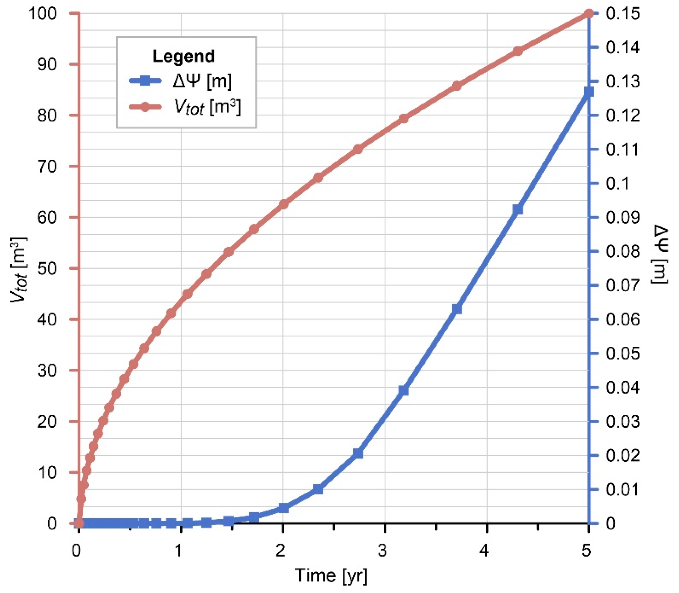
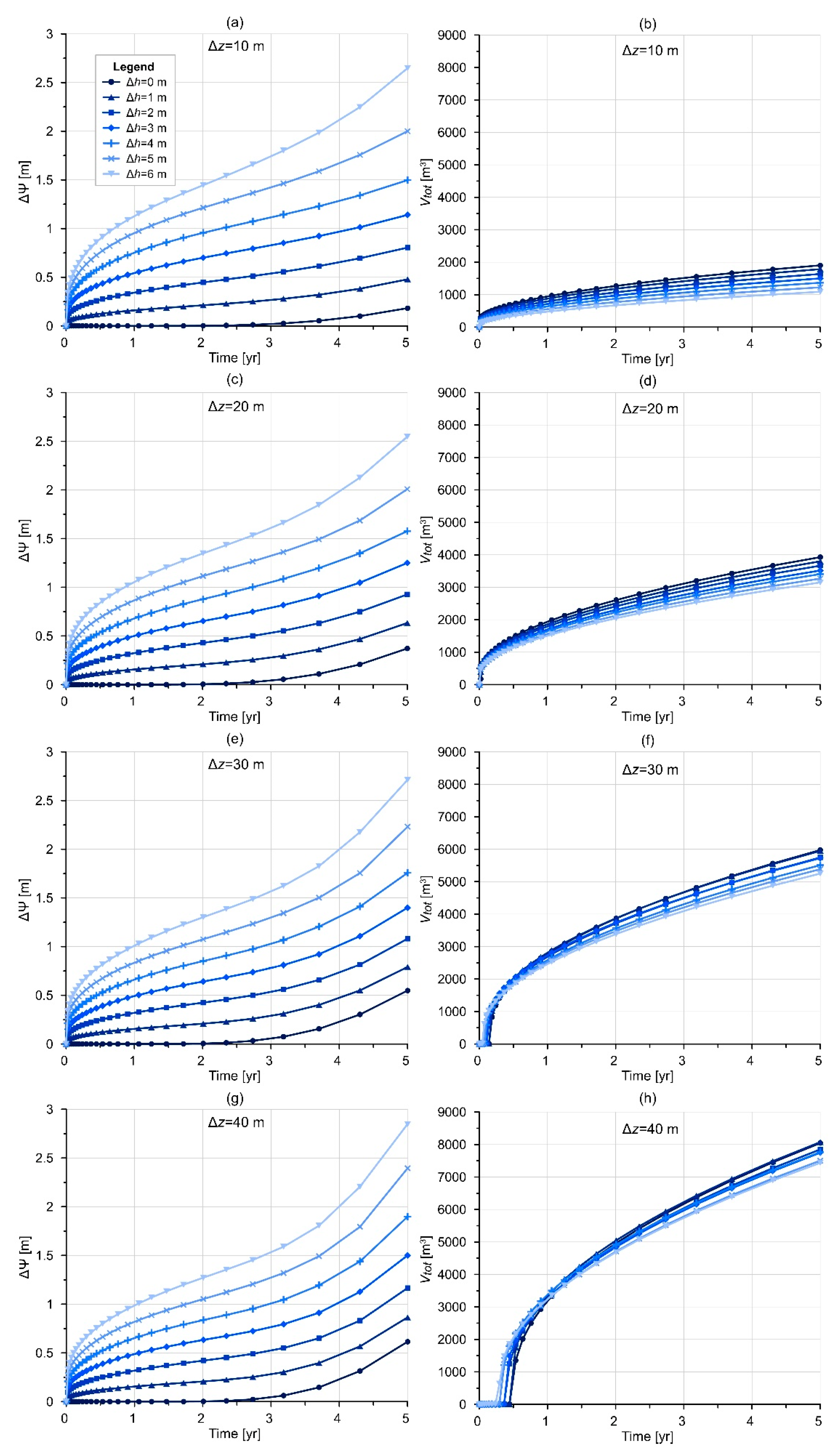
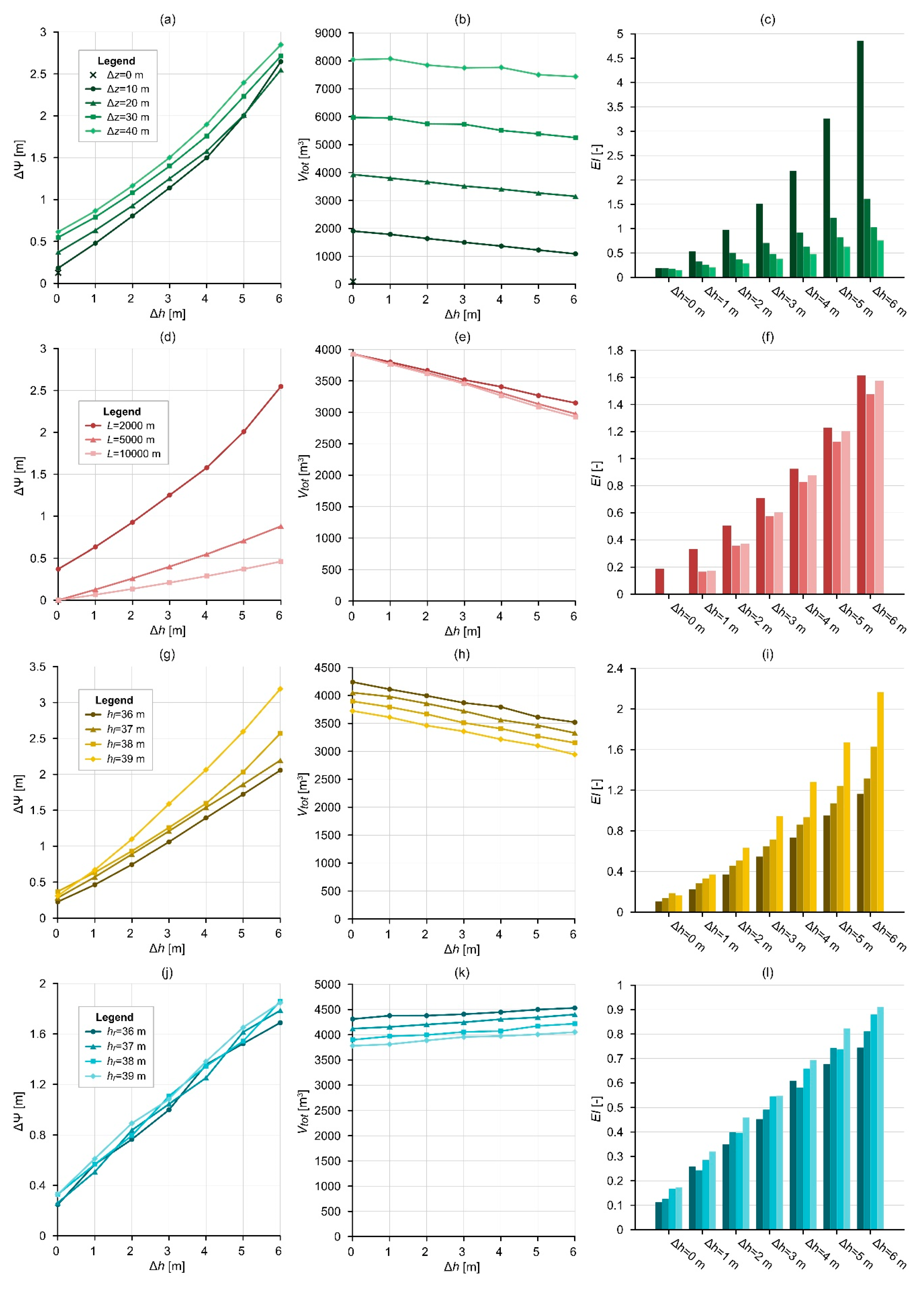
2.2.1. Topography and Hydraulic Head Difference (SG-1)

The first scenario is where the topography is flat (Δz = 0 m) and the water level does not have any changes (Δh = 0 m). Here, the water level is at 2 m depth everywhere along the cross-section (L = 2000 m). Figure 2 illustrates the water level increase on the left side of the model (ΔΨ) and the cumulative amount of water infiltrated from the infiltration basin (V_tot) in time. It shows that the water level starts to increase visibly after approx. 1.5 years and reaches an increase of the order of 0.1 m. By maintaining a 1 m water column in the basin, 100 m³ of water infiltrates from the basin within five years (Figure 2). The infiltration is more rapid at the beginning, and then the process starts to slow down.

For SG-1, seven different scenario types were created, changing Δh values between 0 and 6 m to follow the effect of groundwater table inclination (Table 1). Each of these scenarios was run with different topography, where Δz ranged from 0 to 40 m, creating 29 scenarios in total. (Note: scenarios with no slope in topography, but when the hydraulic gradient was higher than zero, were not considered in this study, as they do not represent real conditions.)

Water level increase starts sooner for the scenarios with Δh = 6 m than for those with Δh = 0 m (Figure 3a,c,e,g). For the latter ones, it takes two to three years to show a visible difference. The main infiltration phase occurs later in case of higher topographic differences (Figure 3b,d,e,h). In the case of Δz = 40 m (Figure 3h), it starts between 100 and 200 days, depending on Δh.

Water level increase after five years ranged from 0.13 m to 0.61 m for the scenarios with Δh = 0 m and ranged from 2.55 m to 2.85 m for the scenarios with Δh = 6 m (Figure 4a). The results related to Δz = 10 m showed the lowest values in general, while the highest ones were noticed in connection with Δz = 40 m (Figure 4a). Concerning the infiltrating water amount in five years, V_tot ranges between 1089–1903 m³, 3149–3928 m³, 5251–5975 m³, and 7435–8045 m³ for Δz = 10, 20, 30, and 40 m, respectively. In every case, the highest V_tot values are related to the lowest Δh values (Figure 4b). Overall, the scenarios described by Δh = 0 m show the lowest efficiency values (EI = 0.15–0.19), while the highest ones are connected to those scenarios with Δh = 6 m (EI = 0.76–4.86). Higher Δz resulted in lower efficiencies, and these differences are more significant for higher Δh values (Figure 4c).

2.2.2. Model Length (SG-2)

Different model lengths represent the different distances between the recharge area (the location of the MAR system) and the discharge area (the location of a groundwater-dependent ecosystem). Three scenarios were tested in this regard with a length of 2000 m, 5000 m, and 10,000 m. The hydraulic head difference ranged between 0 and 6 m, while the depth of the model (D = 40 m) and the topography (Δz = 20 m) were constant (Table 1).

Water level increase ranged between 0.37–2.55 m, 0–0.88 m, and 0–0.46 m for the scenarios with lengths of 2000, 5000, and 10,000 m, respectively (Figure 4d). The infiltrated water amount is similar for all the scenarios. The highest difference can be noticed in the case of Δh = 6 m, where V_tot is 3149 m³, 2976 m³, and 2926 m³ for the scenarios with L = 2000, 5000, and 10,000 m, respectively (Figure 4e). The highest efficiencies (EI = 0.19–1.62) are related to the smallest model (L = 2000 m); however, the other two scenario types (L = 5000 m and L = 10,000 m) can be similarly efficient (EI = 0–1.48 and EI = 0–1.58; Figure 4f). Regarding different Δh scenarios, similar patterns can be noticed with SG-1.

2.2.3. Elevation of Water Table (SG-3)

The aim of changing the position of the water table was to understand how this parameter influences the obtained results regarding different Δh scenarios (Δh = 0–6 m). For these scenarios, the topography and the model length were fixed (Δz = 20 m, L = 2000 m). Two main scenario groups were created: (i) SG-3/A, where the hydraulic head on the left side (h_l) was changed between 36–39 m (meaning, 4–1 m water depth on the left side), in this case, h_r changed based on Δh; (ii) SG-3/B, where the hydraulic head on the right side was changed (h_r) between 36–39 m (meaning, 22–19 m water depth on the right side), in this case, h_l changed based on Δh (Table 1). These parameters were specified for the steady-state models determining the initial conditions.

For SG-3/A, water level increase ranged between 0.23–2.06 m, 0.28–2.2 m, 0.37–2.57, and 0.31–3.19 m for the scenarios with h_l values of 36, 37, 38, and 39 m, respectively (Figure 4g). The results related to Δh = 0 m showed the lowest ΔΨ values, while the highest ones were noticed in connection with Δh = 6 m. V_tot ranges between 3521–4241 m³, 3329–4051 m³, 3152–3895 m³, and 2942–3724 m³ for h_l = 36, 37, 38, 39 m, respectively. In every case, the highest V_tot values are related to the lowest Δh values (Figure 4h). In general, EI was lower for scenarios with a deeper water table (h_l = 36 m, EI = 0.11–1.17), and it was higher for scenarios with a higher water table (h_l = 39 m, EI = 0.17–2.17) (Figure 4i).

For SG-3/B, ΔΨ values are similar for all scenario types (h_r values of 36, 37, 38, and 39 m) and change only with respect to Δh (Figure 4j). The results related to Δh = 0 m showed the lowest values (ΔΨ = 0.25–0.33 m), while the highest ones were noticed in connection with Δh = 6 m (ΔΨ = 1.69–1.85 m). V_tot ranges between 4311–4532 m³, 4121–4402 m³, 3899–4219 m³, and 3781–4051 m³ for h_r = 36, 37, 38, and 39 m, respectively. In this case, the highest V_tot values are related to the highest Δh values (Figure 4k), contrary to the results obtained for SG-3/A. In general, EI was lower for scenarios with a deeper water table (h_r = 36 m, EI = 0.11–0.75) and higher for scenarios with a higher water table (h_r = 39 m, EI = 0.17–0.91). Regarding different Δh scenarios, similar patterns can be noticed with SG-1 (Figure 4l), both in the case of SG-3/A and SG-3/B.

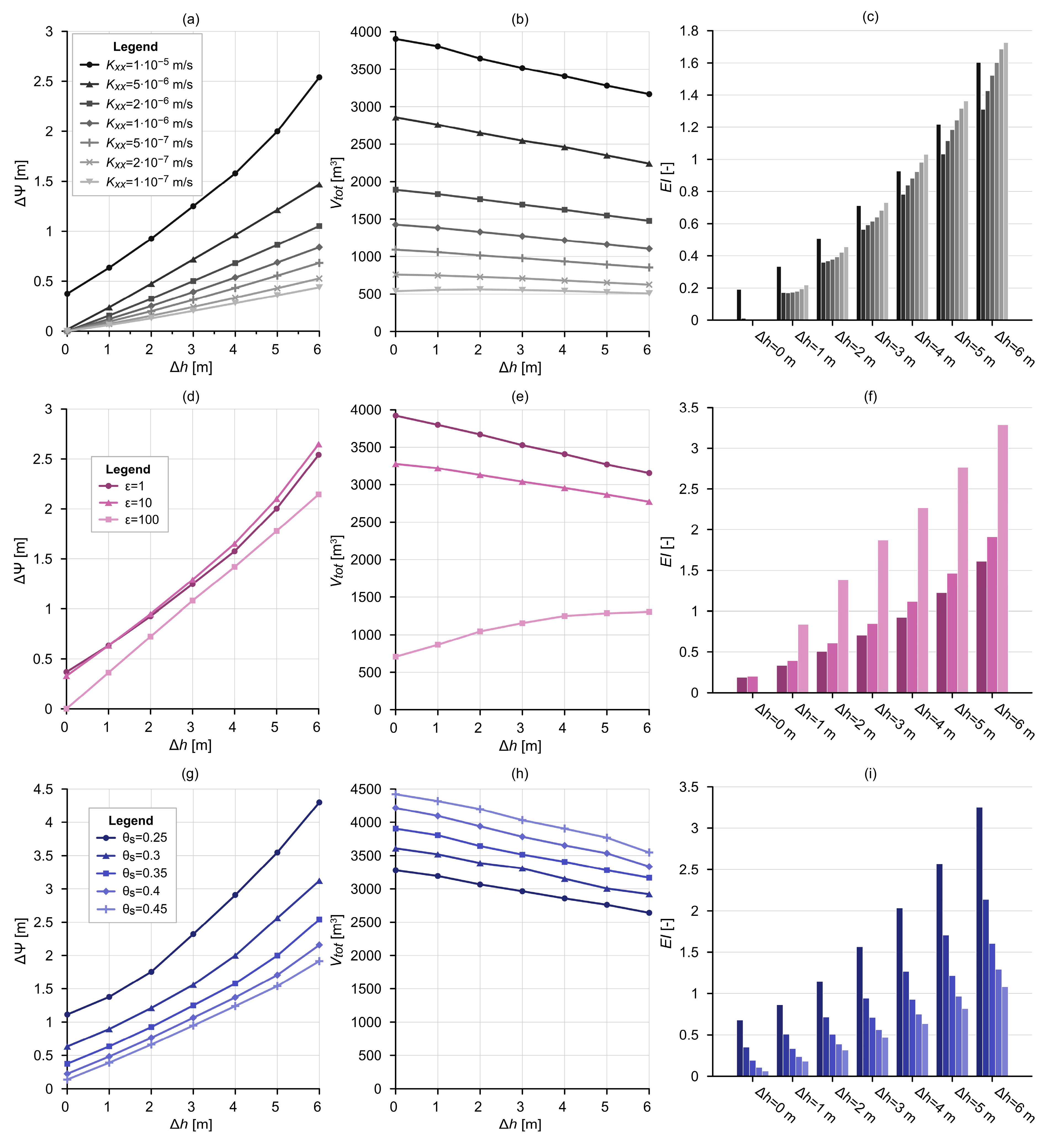
2.2.4. Material Properties (SG-4)

Variation in material properties was investigated to reveal their influence on the efficiency of water replenishment. The horizontal hydraulic conductivity (K_xx), anisotropy coefficient (ε), and saturated water content (θ_s) were varied separately, creating SG-4/A, SG-4/B, and SG-4/C, respectively (Table 1). For these scenarios, the topography, the model length, and the water level at the left side were fixed (Δz = 20 m, L = 2000 m, h_l = 38 m), and Δh changed between 0 and 6 m.

The horizontal hydraulic conductivity was changed between 1∙10⁻⁷ m/s and 1∙10⁻⁵ m/s (SG-4/A). Water level increase after five years ranged from 0 m to 0.37 m for the scenarios with Δh = 0 m and ranged from 0.44 m to 2.54 m for the scenarios with Δh = 6 m (Figure 5a). The results related to K_xx = 1∙10⁻⁷ m/s showed the lowest values, while the highest ones were noticed in connection with K_xx = 1∙10⁻⁵ m/s (Figure 5a). Concerning the infiltrating water amount in five years, V_tot ranged between 3168–3904 m³ and 508–539 m³ for the scenarios with horizontal hydraulic conductivities of 1∙10⁻⁵ m/s and 1∙10⁻⁷ m/s, respectively. The highest V_tot values are related to the lowest Δh values, in general (Figure 5b). In most cases, the highest EI values were noticed in connection with K_xx = 1∙10⁻⁵ m/s (EI = 0.19–1.6); however, with higher Δh values, lower K_xx values could also result in high efficiency indices (e.g., Δh = 6 m K_xx = 1∙10⁻⁷ m/s, EI = 1.73; Figure 5c).

The anisotropy coefficient (ε) varied between 1 and 100, which means that the vertical hydraulic conductivity was decreased compared to the horizontal hydraulic conductivity (Table 1). Water level increase ranged between 0.37–2.54 m, 0.33–2.65 m and 0–2.14 m for the scenarios with the anisotropy coefficients of 1, 10, and 100, respectively (Figure 5d). Concerning the infiltrating water amount in five years, V_tot ranged between 3153–3919 m³, 2772–3278 m³, and 706–1305 m³ for ε = 1, 10, 100, respectively (Figure 5e). Compared to the other two scenario types, for those with ε = 100, they showed increasing V_tot with increasing hydraulic head difference. Apart from Δh = 0 m, the highest efficiencies are related to ε = 100 (EI = 0.84–3.29), and the lowest ones are related to ε = 1 (EI = 0.19–1.61; Figure 5f).

The water content is an important governing factor of groundwater flow in the unsaturated zone; thus, the saturated water content was tested as well. The saturated water content changed between 0.25 and 0.45. Water level increase after five years ranged from 0.14 m to 1.19 m for the scenarios with Δh = 0 m and ranged from 1.92 m to 4.3 m for the scenarios with Δh = 6 m (Figure 5g). The results related to θ_s = 0.45 showed the lowest values, while the highest ones were noticed in connection with θ_s = 0.25 (Figure 5g). Concerning the infiltrating water amount in five years, V_tot ranged between 2642–3279 m³ and 3546–4421 m³ for the scenarios with a saturated water content of 0.25 and 0.45, respectively. The highest V_tot values are related to the highest θ_s and lowest Δh values (Figure 5h). The highest EI values were noticed in connection with θ_s = 0.25 (EI = 0.68–3.25), and the lowest were noticed in connection with θ_s = 0.45 (EI = 0.06–1.08; Figure 5i). Regarding different Δh scenarios, similar patterns can be noticed for SG-1 (Figure 4l) in all three scenario groups (SG-4/A, SG-4/B, SG-4/C).

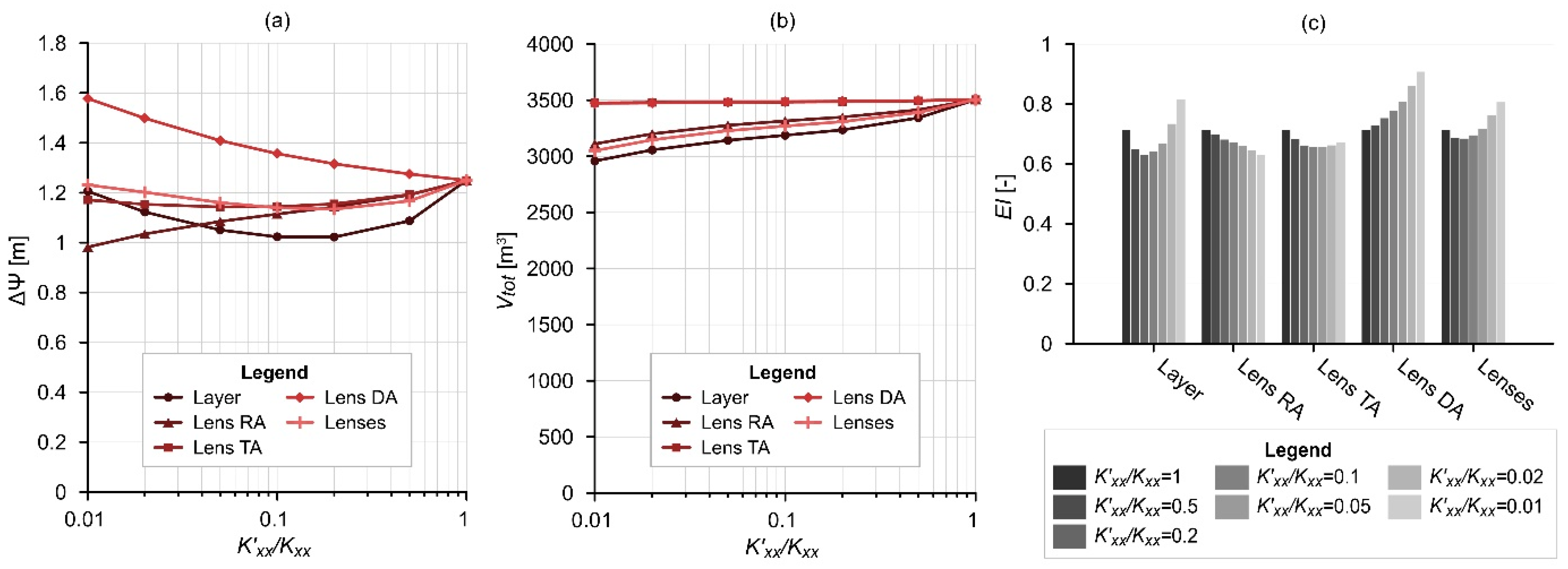
2.2.5. Heterogeneity (SG-5)

The effect of heterogeneity was analysed by creating five different geometries (see Figure 1d for details):

• with a continuous layer (“Layer”);
• with a lens below the recharge area (“Lens RA”);
• with a lens below the throughflow area (“Lens TA”);
• with a lens below the discharge area (“Lens DA”);
• with all three of these lenses (“Lenses”).

The hydraulic conductivity of the main model domain was kept at K_xx = 1∙10⁻⁵ m/s, while K’_xx was changed between 1∙10⁻⁵ and 1∙10⁻⁷ m/s for the intersecting layer and lenses. For these scenarios, the topography, the model length, the water level at the left side, as well as the hydraulic head difference, were fixed (Δz = 20 m, L = 2000 m, h_l = 38 m, Δh = 3 m).

For most of the scenarios, water level increase ranged between 0.98 m and 1.25 m, while for “Lens DA”, it ranged between 1.25 m and 1.58 m, showing an increasing trend towards lower K’_xx/K_xx ratios (Figure 6a). For “Lens DA” and “Lens TA”, V_tot ranged between 3472–3505 m³. In the case of the other three scenario types, it varied between 2958 m³ and 3505 m³, showing an increasing trend towards higher K’_xx/K_xx ratios (Figure 6b). The Efficiency Indices were similar (EI = 0.63–0.91), “Lense RA” showed a decreasing trend, and “Lense DA” showed an increasing trend towards lower K’_xx/K_xx ratios (Figure 6c).

2.2.6. Parameters of the Infiltration Basin (SG-6)

The aim of changing the infiltration basin parameters was to understand their effect on the water level increase and their efficiency regarding water replenishment. The basin width (w) and the water depth in the infiltration basin (d) were varied separately, creating SG-6/A and SG-6/B, respectively (Table 1). For these scenarios, all other parameters were constant, except for Δh, which varied between 0 and 6 m, similar to SG-1–4.

The width of the basin was cut to half and was doubled (w = 50, 100, 150 m). Water level increase after five years ranged between 0.3–2.44 m, 0.37–2.54 m, and 0.46–2.66 m for the scenarios with a width of 50, 100, and 150 m, respectively (Figure 7a). In every case, the highest ΔΨ values are related to the highest Δh values. Concerning the infiltrating water amount in five years, V_tot ranges between 2929–3633 m³, 3168–3904 m³ and 3375–4162 for w = 50, 100, and 150 m, respectively (Figure 7b). In every case, the highest V_tot values are related to the lowest Δh values. Below Δh = 2 m, the scenarios described by w = 50 m showed the lowest efficiency values (EI = 0.17–0.32), and the ones with w = 150 m showed the highest ones (EI = 0.22–0.35). However, above Δh = 2 m, this relationship is reversed: the scenarios with w = 50 m resulted in the highest EI values (EI = 0.73–1.66), and the ones with w = 150 m showed the lowest efficiencies (EI = 0.7–1.57; Figure 7c). Regarding different Δh scenarios, similar patterns can be noticed to SG-1.

Four different scenarios were investigated regarding water column height in the basin: 0.5, 1, 1.5, and 2 m. In the case of the latter one, the basin was completely full. Water level increase after five years ranged between 0.35–2.51 m, 0.37–2.54 m, 0.39–2.57 m, and 0.4–2.6 m for the scenarios with a water depth of 0.5, 1, 1.5, and 2 m, respectively (Figure 7d). In every case, the highest ΔΨ values are related to the highest Δh values. Regarding the cumulative volume of infiltrated water in five years, V_tot ranges between 3063–3821 m³, 3168–3904 m³, 3225–3983 m³, and 3293–4069 m³ for d = 0.5, 1, 1.5, and 2 m, respectively. In every case, the highest V_tot values are related to the lowest Δh values (Figure 7e). Below Δh = 2 m, the scenarios showed similar Efficiency Indices (EI = 0.18–0.2 for Δh = 0 m and EI = 0.33 for Δh = 1 m); however, above Δh = 2 m, a decrease in EI was noticed towards higher d values (EI = 0.51–1.64 for d = 0.5 m and EI = 0.49–1.58 for d = 2 m; Figure 7f). Regarding different Δh scenarios, similar patterns can be noticed for SG-1.

2.3. Interpretation

The simulated scenarios have demonstrated the effect of groundwater table inclination on infiltration-based MAR efficiency in a simple groundwater basin (with one recharge and one discharge area). The obtained results revealed the significance of the hydraulic gradient. Higher initial hydraulic gradients (i.e., increasing Δh) induced a higher water level increase at the discharge area (ΔΨ, Figure 3a,c,e,g and Figure 4a). The achieved water level increase is approx. one order of magnitude higher in the case of Δh = 6 m than in the case of Δh = 0 m (Figure 4a). At the beginning of the modelling period (t = 0 yr), the difference between the results is slight, and in the course of time, it becomes more significant (Figure 3a,c,e,g). On the other hand, higher topography slopes (i.e., increasing Δz) induce only a slightly higher ΔΨ in five years (Figure 4a). Increasing water level on the left-hand side can be explained by a higher induced hydraulic gradient between the infiltration basin and the discharge area. This phenomenon was noticed in the case of every scenario group, where Δh was changed (SG-1–4, SG-6).

Increasing the hydraulic head difference caused a slight decrease in the amount of cumulative water volume (V_tot, e.g., Figure 4b,e,h) infiltrating from the infiltration basin. On the other hand, by comparing scenarios with different topography, more significant changes can be noticed (Figure 4b). In the case of Δh = 6 m, there is a sevenfold difference between the cumulative water volume (V_tot = 1089 m³ and 7435 m³) related to the scenarios with Δz = 10 m and Δz = 40 m, respectively (Figure 4b). These differences can be explained by the storage capacity of the model domain. Higher Δz means a thicker unsaturated zone, thus more water can be stored, and it takes more time for the infiltrated water to reach the initial water table. As h_l is initially fixed in these cases, h_r changes based on Δh. In the case of Δh = 6 m, h_r is closer to the surface, causing a thinner unsaturated zone. This way, water reaches the saturated zone sooner than in the case of Δh = 0 m.

Comparing the achieved water level increase in five years for the different scenarios, the results show that Δh is an important factor in increasing the water level downgradient and has a stronger effect on water level increase than Δz (Figure 4a). However, the amount of water recharging from the infiltration basin is influenced considerably by the topography (Δz), i.e., the thickness of the unsaturated zone (Figure 4b). The efficiency index (EI) is increased by increasing hydraulic gradient (Δh), while it is decreased by higher surface elevations (Δz) (Figure 4c).

Considering different model lengths (L, SG-2), the higher the distance between the infiltration and the discharge area, the lower the water level increase achieved in five years. However, the EI, which represents the whole model domain (by involving L in Equation (3)), shows similar results in each case, indicating that this can be an efficient method, regardless of distance.

The relative position of the water table (SG-3) had an effect on the obtained results as well. When it is closer to the surface on the left side (h_l), the water level increase is higher than in the case of deeper water tables (Figure 4g). The difference is especially significant in the case of h_l = 39 m, where the water level is only in 1 m depth. The model set-up and the boundary conditions possibly induce this phenomenon. On the other hand, no significant difference can be observed in the water level increase achieved after five years if the initial hydraulic head on the right side of the model (h_r) is changed (Figure 4j). The different Δh values had an effect on the water level increase in each case (SG-3/A and SG-3/B): higher Δh caused a higher water level increase. The cumulative water volume is slightly higher when the water table is deeper (Figure 4h,k), which can be explained by higher storage capacity. While, in the case of SG-3/A, higher Δh induced a lower amount of water infiltration (Figure 4h), and, for SG-3/B, a slight increase can be noticed by increasing Δh (Figure 4k). This difference is connected to storage capacity, as well. When h_r was fixed (SG-3/B, e.g., h_r = 38 m), Δh = 6 m meant a deeper water table at the left side (h_l = 32 m), thus representing higher storage capacity than in the case of Δh = 0 m (h_l = 38 m). For SG-3A, this is the other way around. Both in the case of SG-3/A and SG-3/B, efficiency indices were higher when the water table was closer to the surface (Figure 4i,l).

Regarding material properties (SG-4), horizontal hydraulic conductivity had a significant effect on both ΔΨ and V_tot. Model scenarios with higher K_xx values induced higher water level increases (Figure 5a). Almost one order of magnitude difference was noticed between the scenarios with K_xx = 1∙10⁻⁷ m/s and K_xx = 1∙10⁻⁵ m/s. The infiltrated water volume after five years also increased with higher K_xx values (Figure 5b). Efficiency indices of SG-4/A (Figure 5c) show that even smaller hydraulic conductivity values can be enough to reach sufficient water level increase downgradient with a lower amount of water infiltration.

A smaller water level increase was achieved with higher ε (Figure 5d). It had an even stronger effect on the infiltrated water amount: the difference between the scenarios with ε = 100 and ε = 1 was approx. threefold (Figure 5e). Due to these differences in most cases, higher ε resulted in higher EI (Figure 5f). If the aim of water infiltration is to increase the water level at the discharge area, lower vertical hydraulic conductivity (i.e., higher ε) can be beneficial, as the infiltrated water tends to move laterally instead.

Increasing θ_s resulted in a lower water level increase after five years (Figure 5d) while inducing a higher amount of infiltration (Figure 5e). These processes can be explained by higher porosity. Thus, the higher storage capacity of the modelling framework is represented. Consequently, the efficiency was the highest in the case of the lowest θ_s value (Figure 5f) from the perspective of GDE rehabilitation.

Concerning heterogeneities (SG-5) in the model framework, the highest water level increase could be achieved by the lens below the discharge area, especially in the case it had a low hydraulic conductivity, while the layer or the lens below the recharge area induced a smaller water level increase (Figure 6a). The cumulative water volume infiltrating from the basin was quite similar for all the scenarios with “Lens DA” and “Lens TA” showing the highest values (Figure 6b). Efficiency indices show that the lens below the discharge area can be beneficial for water replenishment, while if it is located below the recharge area, it can cause lower efficiency (Figure 6c). The efficiency of other geometries, such as the layer, depends on their hydraulic conductivity.

Compared to the previous parameters, the characteristics of the infiltration basin (SG-6) had a negligible effect on the obtained results. The widest infiltration basin (w = 150 m) and the one with the highest water column (d = 2 m) caused the highest water level increase on the left side of the model (Figure 7a,d); however, the differences between the ΔΨ values were minimal. Basin parameters also had a slight impact on the cumulative water volume infiltrated in five years (Figure 7b,e), increasing w and d, which resulted in slightly higher values. The efficiency indices showed that, with higher initial hydraulic head differences (above dh = 2 m), smaller infiltration basins and lower water columns in the basin could be slightly more efficient (Figure 7c,f). The small difference between these scenarios suggests that careful planning must be carried out in order to optimise the implementation and operation of MAR projects.

3. Case Study

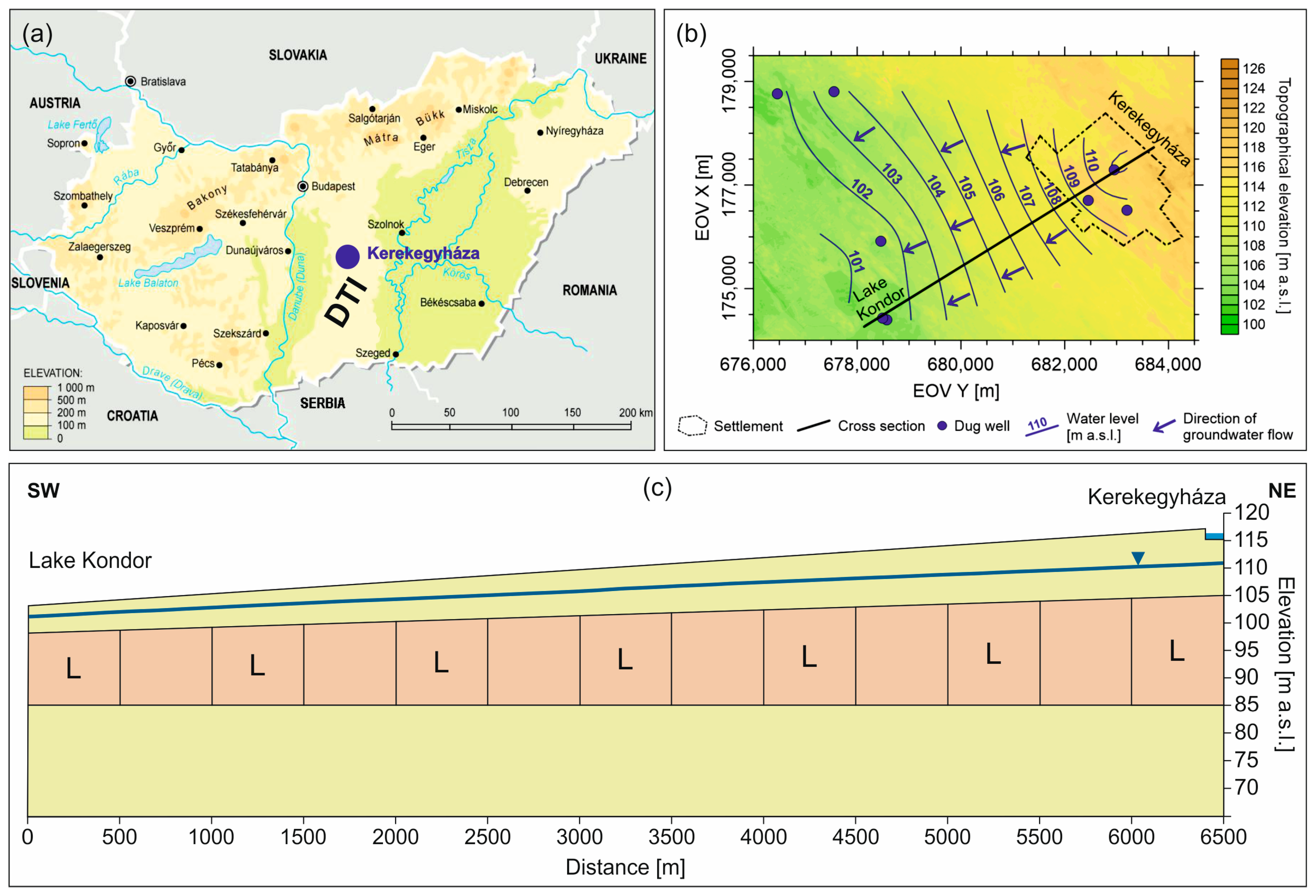
3.1. Study Area

For the demonstration of the significance of groundwater table inclination and the applicability of these MAR settings for GDE replenishment, a case study was selected, and a simple basin was delineated, which reflects a close-to-real situation. The study area is located in Hungary, in the Danube-Tisza Interfluve (DTI), which is an elevated ridge region situated between the Danube and Tisza rivers (Figure 8). This is one of the biggest alluvial (cone) plains in the Great Hungarian Plain, created by the Ancient Danube in the Late Pliocene and Pleistocene. After the area had filled up, the Danube riverbed was relocated, and a strong aeolian sediment accumulation begun, creating sand dunes [69,70,71].

Water level decline started in the 1970s in the area [72], which induced a series of water-related problems: wells drying up, less available water for agriculture, disappearance of GDEs, and further socio-economic and ecological problems [73]. The causes of the water level decrease are complex, and the negative trend can both be attributed to climate change, as well as to canalisation, groundwater abstraction, land use changes, and land drainage [73,74,75]. These processes, together, caused a 2–3 m water level decline on average. However, in some areas, it even reached 6–7 m [76]. Although several plans have been prepared in the last decades to address water scarcity, the problem is still unresolved. Different replenishment scenarios were made for channelling river water from the Danube to the area either by connecting the Danube and Tisza rivers with a navigable canal or by pumping water through the existing canal network and/or newly constructed pipes (e.g., [77,78,79]). Others saw the solution in constructing reservoirs [79,80,81], even taking into consideration using them for infiltration. However, managed aquifer recharge as a potential solution has not been considered yet.

One of the lakes that dried up in the ridge region is Lake Kondor [82], which is located close to Kerekegyháza, a small rural town in the DTI area (Figure 8a,b). The lake is located approximately 5 km downgradient from the settlement. This area was selected for the purpose of the numerical simulations considering that the settlement is located on an elevated area and the lake was present in a local discharge area before it dried up [83].

3.2. Numerical Settings

As a first step, a simple basin was delineated (Figure 8) between the town (recharge) and the dried-up lake (discharge) on the basis of previous studies for the DTI [83].

Based on the results of the theoretical simulations, a test model was created to examine the influence of near-surface groundwater flow on the efficiency of infiltration-based MAR for the goals of GDE rehabilitation (Table 1). The simulated cross-section displays the main characters of the area regarding topography and hydrostratigraphy and serves only to demonstrate the applicability of the concept.

The length (L) of the model was 6500 m, the depth (D) was 38 m on the left side, and the depth was 52 m on the right side (Figure 8c). The topography was linearly increasing from 103 m to 117 m (simplified from the digital elevation model acquired from the Lechner Knowledge Centre with a resolution of 5 m). The upper part of the model (Z > 85 m) had a 2.5 m average mesh size. The lower part of the model (Z = 65–85 m) had a less detailed mesh with a 10 m average mesh size. The number of elements was 32,704.

The geology of the research area is composed of alluvial and aeolian sediments, such as sand, silt, loess, clay, and their variations [84]. The geology is quite heterogeneous with alternating silty and sandy lenses [85], thus it had to be simplified. Three different scenarios were tested considering the theoretical models and the diverse geology (Figure 8c) using the results of Oláh [85], Yousif [86], and Szabó et al. [87] for the study area:

• “K-1”: A homogeneous model with horizontal hydraulic conductivity (K_xx) of 5∙10⁻⁶ m/s.
• “K-2”: A model with three layers, where the upper and lower layers were described by K_xx = 5∙10⁻⁶ m/s and the middle layer by K_xx = 5∙10⁻⁷ m/s. The upper layer was 5 m thick on the left side and 10 m thick on the right side; the bottom of the middle layer was at 85 m a.s.l.
• “K-3”: A model with lenses, where the model domain and the lenses were characterised by K_xx = 5∙10⁻⁶ m/s and K_xx = 5∙10⁻⁷ m/s, respectively.

Similarly to the theoretical models, the model domain was kept as isotropic, the saturated water content (θ_s) was 0.35, the residual water content (θ_r) was defined as 0.035, and the in-built silty sand sample curve was used for the estimation of volumetric water content function.

The boundary conditions were defined similarly to the theoretical models: a steady-state model provided the initial hydraulic head conditions for the transient model. As a first step, a steady-state model was built, where h_l = 101 m (2 m below the surface) and h_r = 111 m. Thus, the hydraulic gradient is approx. 0.0015, similar to the scenarios where the length of the model was 2000 m and Δh was 3 m (SG-1, SG-3–6). A transient model of 50 years (18,250 days) was built with 200 exponentially increasing steps. For the transient model, h_l and h_r were not specified, and it used the steady-state model to acquire initial hydraulic head conditions. The infiltration basin was identical to the ones presented in SG-1–5 and was defined in the same way.

3.3. Results

The results of the transient simulations display that the position of the water level is increasing continuously in time on the left side of the model (Lake Kondor), reaching approx. 2.09, 1.63, and 1.93 m after 25 years and 3.15, 2.39, and 2.77 m after 50 years for K-1, K-2, and K-3 scenarios, respectively (Figure 9a). The water level reached the ground surface in approx. 23, 37, and 27 years, respectively.

The cumulative water volume infiltrating from the basin in 50 years is approx. 2413, 1871, and 2048 m³ for K-1, K-2, and K-3 scenarios (Figure 9b).

The efficiency index (EI) was calculated for every time step to understand its behaviour in time. In the beginning, the EI decreases rapidly, then after approx. 15–20 years, it remains fairly stable, especially in the case of the homogeneous and layered models (Figure 9c). Overall, K-3 showed the highest efficiency.

On the cross-section displaying the scenario with lenses (K-3, Figure 9d), the highest water level increase can be noticed around Kerekegyháza settlement (recharge area). After 25 years, the water level almost reached the surface at the discharge area, and after 50 years, water reappeared on the surface. The water level only slightly increased in the middle of the model during the modelling time.

3.4. Interpretation

The case study revealed similar findings to the theoretical models. Even with a higher distance (in this case L = 6500 m) between the recharge and discharge area, the water table can be visibly increased within a reasonable time (Figure 9d). It also confirmed that material properties and heterogeneity have a strong effect on the obtained results and can highly influence the time it is needed for the water table to reach the surface again (Figure 9a). While the homogeneous model reached the highest water table increase in 50 years (Figure 9a), the model with lenses was the most efficient from the point of view of ecosystem restoration (Figure 9c), as smaller amount of water infiltrated to achieve that (Figure 9b).

4. Discussion

4.1. Relevance and Limitations of the Theoretical Models

Although the importance of water table inclination or hydraulic gradient was not systematically investigated previously in connection with managed aquifer recharge, the theoretical model results of this study showed its significance and are the first step to understand the effect of recharge dynamics on MAR performance.

Higher initial hydraulic head difference initiated the strongest driving force and influenced the achieved water level increase in a positive way. In all the cases, the highest Δh values caused the highest efficiency indices, which clearly indicates the significance of this parameter.

Based on Darcy’s Law, the flux of groundwater flow in the saturated zone depends on the hydraulic gradient (Δh/L) and on the saturated hydraulic conductivity (K) of the aquifer [67]. We could reveal that, in addition to hydraulic gradient, hydraulic conductivity, consequently anisotropy (ε), and heterogeneity have the highest impact on the achieved water level increase at the discharge area.

Regarding the cumulative water amount infiltrating from the basin during the modelling period, the majority of the differences can be explained by storage capacity under the recharge area where the basin was settled. The parameters that had a significant effect in this regard are the topography (Δz) and water table depth, including the thickness of the unsaturated zone and the material properties of the model domain, such as hydraulic conductivity (K), anisotropy (ε), and saturated water content (θ_s). Heterogeneity plays a role in this regard, especially in those cases when there is a layer or lens with lower hydraulic conductivity below the recharge area. The results of this research are in accordance with the ones acquired by Wu et al. [88], who investigated the effects of geological heterogeneity on MAR efficiency.

These parameters are also important in those cases, when the aim of MAR implementation is permanent water storage in an aquifer (specially to prevent water mixing in brackish aquifers). From this point of view, exactly the opposite conditions are needed [23,24,58].

The hydrogeological delineation of adequate basins and theoretical models help the optimisation of MAR projects by offering solutions for the most efficient scenarios for groundwater level increase and ecosystem rehabilitation, and they further help to avoid negative effects, such as unwanted flooding of any area. Higher hydraulic conductivity, higher hydraulic gradient, and smaller distance between the recharge and discharge area or shallower water table could result in quicker water level increase. Thus, one must be cautious while designing MAR systems.

The modelling study has several limitations. Maintaining 1 m water level in the infiltration basin is theoretically possible, but in reality, the water source used for infiltration is not always available, and there might be seasonal differences (e.g., [89]). Precipitation, evaporation, and clogging were not investigated; however, they can have an impact on the amount of water needed in total and on the achieved water levels [35,90,91,92,93]. Thus, the volumetric water volume values display an ideal case and only serve the purpose of comparison in this research. For calculating the whole amount of water needed for water replenishment, three-dimensional models, including more complex processes, are needed. For a preliminary estimation, the results can be upscaled. In this study, a one-meter element thickness was used; thus, the results can be easily upscaled to the desired distance.

The initial water level generates a hydraulic gradient (in the case of the scenarios with Δh > 0 m); thus, a minor imbalance occurs in the water levels (0–0.2 m) in the first few time steps of the model (0–50 days, depending on the scenarios) until the infiltration from the basin takes effect on the groundwater level. For this reason, the results are less reliable in the first two months than those obtained later in the modelling time. This does not affect significantly the results of this research, as they are interpreted considerably later in time (t = 5 years).

The defined efficiency index can be a useful tool to compare different scenarios; however, it should be interpreted within certain limits. As an example, the scenario where K_xx = 1∙10⁻⁷ m/s and Δh = 6 m can seem to be highly efficient (EI = 1.73; SG-4/A, Figure 5c), because only 508 m³ water was enough to increase the water level by 0.44 m in five years. However, one must ask if a 0.44 m water level increase is enough to reach the aims of implementing the MAR system. Thus, specifying the aims of the project during the planning phase is essential both in terms of water level increase and time. The EI can be used in the context of realistic scenarios considering the available source water and the spatial extent of the project.

The used models were adequate to analyse the effect of groundwater table inclination on MAR operation in a simple basin. GeoStudio SEEP/W [65] can be best applied to smaller-scale engineering problems and to evaluate the effect of local processes. However, to involve the impact of groundwater flow systems (considering detailed geology, topography, and recharge conditions) and different groundwater flow regimes (recharge, throughflow, and discharge areas) in MAR design, more complex models are needed. This aspect should be investigated in the future, as it can be a major influencing factor in any case, especially when basin-scale water management schemes are planned [94]. MODFLOW [95], FEFLOW [96], or COMSOL [97] modelling software tools, among others, are more applicable for larger scale models for investigating the effects and efficiency of MAR systems [38,98,99,100], even from the perspective of groundwater flow systems.

4.2. The Relevance and Limitations of the Case Study

The case study proved that the theory could be applied to real-life scenarios as well, and it is worth considering this method as a potential water replenishment measure in the area. This is especially important when considering its advantages compared to the previously offered solutions for the area’s water problems.

One of the plans in the Danube-Tisza Interfluve area was to move water from the Danube valley to the centre of the ridge through existing channels and lakes [79]. The project was expected to replace 14 million m³ of ecological water demand per year and to raise the groundwater level by 0.5–1.5 m near the reservoirs. The most significant problem is that the ridge region is topographically higher than the rivers and larger channels in the valleys, so the water has to be pumped up, which is quite expensive. Furthermore, the water can easily infiltrate from the channels, and it would not reach the higher regions in sufficient amounts.

Another concern is water quality. The lakes of the DTI area have distinct water compositions with different ecosystems, depending on their position in the complex groundwater flow systems of the area [83,101]. Thus, direct recharge of these lakes from surface river water is avoidable, and replenishment from the same flow systems could be more beneficial, more eco-friendly, and more sustainable in the long run.

In addition, the scale and necessary water need are important factors, as well. The only available natural surplus water in the ridge region originates from rainwater. Alternatively, treated wastewater might be used for infiltration in the future, as well, when the legislative background and adequate protocols are developed for it in the country.

Collecting rainwater from roofs and roads in the settlement located on the elevated part of the basin and using it for the purposeful recharge of groundwater, the water level can be increased, not only under the recharge area, but also in the surroundings of the related discharge regions (Figure 9d). Therefore, less amount of water can be necessary. By using this proposed nature-based approach, similar water quality could be achieved around the discharge area, as it has been before the water level decline. As a whole, the proposed approach can provide a small-scale, diverse, and nature-based solution for settlement-level water management and GDE rehabilitation. It can also be upscaled for the ridge region (DTI). This solution would be more environmentally and economically reliable compared to the previous plans (e.g., [77,79]).

The three evaluated scenarios (K-1, K-2, K-3; Figure 9a) showed that the water level could reach the surface again in 23–37 years, increasing the water table by 2 m. However, the obtained results are highly dependent on the geology of the model. In order to achieve more reliable results in this regard, more detailed geological and geophysical research is needed in the area. In the future, three-dimensional numerical modelling studies involving further processes, such as evapotranspiration, precipitation, and lateral flow rate, could improve the predictions, which could be used for planning purposes. Further investigation is needed to determine the factors which could shorten the time needed for replenishing Lake Kondor. Based on the theoretical model results, the infiltration basin parameters only slightly affect the achieved water level increase, thus the efficiency of other types of methods should be analysed as well. Considering that well recharge methods infiltrate water directly to the saturated zone [3,4,5], these methods might result in faster water level increase at the discharge area.

4.3. Nature-Based Solutions and GDE Replenishment

Water retention at the recharge area, using managed aquifer recharge with water sources, such as rainwater, surface runoff, or even treated wastewater, can also be beneficial on a catchment scale [7]. It can serve as a flood control measure, but as a watershed management approach, as well. Several studies confirmed [8,102,103] that MAR can cause seepage in discharge areas and springs, and it can improve the baseflow of rivers [104], which is in good agreement with the findings of this research. Based on the results of the theoretical and simplified case study models, a conceptual model was built to summarise the proposed approach (Figure 10). As water seeps into the aquifer from the infiltration basin, the water level of the basin connects with the groundwater level and a mound forms below it, thus increasing the water level at the recharge area. This water level increase has an effect on the water level at the discharge area, where the water table starts to rise, as well, due to flow dynamics, i.e., hydraulic continuity [105]. This means that the water level can be increased indirectly and, thus, not the mound formation itself is the cause of the water level increase at the discharge area, but the difference in hydraulic heads between the recharge and discharge areas, caused by the infiltration. In addition, the water level beneficially increases around the recharge and discharge area as well. Intentionally searching for related recharge and discharge areas can help to use this approach during MAR planning and operation. In contrast to the presented simple basins (theoretical models and case study), real basins are characterised by hierarchical flow systems, so their prior investigation is necessary as well.

Based on these considerations, this method can serve as a nature-based solution, as it can accelerate or rehabilitate natural processes regarding groundwater flow and can restore groundwater levels and groundwater-dependent ecosystems in an eco-friendly and sustainable way, especially using rainwater for infiltration. If the initial shallow groundwater quality is non-compliant, rainwater and runoff water infiltration can even improve it in the long run. This approach holds a combined solution applying natural groundwater processes: it may alleviate the periodic availability of surplus water and enhance soil and land moisture due to diverse hydroclimatic extreme events, i.e., floods and droughts, sometimes affecting the same locality. This approach is not only nature-based, but it can be handled as a smart solution as well, because due to the hydraulic solution, the water need for the replenishment and the environmental impacts can be decreased.

5. Conclusions

The evaluation of the theoretical model scenarios and case study scenarios led to the following conclusions:

• The theoretical models for a simple basin revealed the significance of groundwater table inclination for infiltration-based MAR planning and operation.
• The achieved water level increase (ΔΨ) was approx. one order of magnitude higher in the case of higher initial hydraulic head difference (Δh = 6 m) than in the case of Δh = 0 m. In addition, the distance between the recharge and discharge areas and the hydraulic conductivity has the most significant effect on the water level increase at the discharge area.
• The results showed that the amount of water infiltrated from the infiltration basin (V_tot) is principally governed by topographic difference and the depth of water table, thus by the thickness of the unsaturated zone. There was a sevenfold difference between the cumulative water volumes related to the scenarios with Δz = 10 m and Δz = 40 m, in the case of Δh = 6 m. Furthermore, the material properties of the aquifer, such as hydraulic conductivity, anisotropy, saturated water content, and heterogeneity, have an effect on the infiltrated volumes.
• From the perspective of groundwater-dependent ecosystem preservation and restoration, the most efficient scenarios are when the hydraulic gradient and the horizontal hydraulic conductivity are high, and the aquifer has a lower storage capacity. This means that exactly the opposite conditions are required, as in the case of long-term water storage in an aquifer.
• The established efficiency index, involving the achieved water level increase and the infiltrated water volumes, can be used to differentiate between realistic scenarios and to optimise the MAR design in the future.
• The investigated case study proved the applicability and efficiency of the initial concept and offered a possible water management measure for increasing the water reserves and restoring the GDE of the area. The applied approach offers a smart, diverse, and nature-based solution, and it can be advantageous compared to the previously proposed water replenishment plans for the area.
• Based on the results of the theoretical and simplified case study models, a conceptual model was built: if water is infiltrated at the local recharge area (elevated area), the water table will increase at the local discharge area (local topographical depression), as well, due to hydraulic continuity, which can have a positive effect on GDEs, using natural settings and processes. Furthermore, the water level beneficially increases around the recharge and discharge area, as well.

In changing climatic conditions, this approach can serve as a smart and nature-based solution to increase the water table at discharge areas with relatively low amount of recharge water and thereby sustain sensitive ecosystems. In addition, these numerical modelling scenarios can help to better understand MAR efficiency in light of local groundwater flow processes and can contribute to better optimisation of MAR systems in the future.

References

- NRMMC; EPHC; NHMRC. Australian Guidelines for Water Recycling, Managing Health and Environmental Risks, Vol 2C: Managed Aquifer Recharge; Biotext: Canberra, Australia, 2009; 237p. [Google Scholar]
- Bouwer, H. Artificial Recharge of Groundwater: Hydrogeology and Engineering. Hydrogeol. J. 2002, 10, 121–142. [Google Scholar] [CrossRef] [Green Version]
- Gale, I. Strategies for Managed Aquifer Recharge in Semi-Arid Areas; UNESCO: Paris, France, 2005; 30p. [Google Scholar]
- Dillon, P.; Toze, S.; Page, D.; Vanderzalm, J.; Bekele, E.; Sidhu, J.; Rinck-Pfeiffer, S. Managed Aquifer Recharge: Rediscovering Nature as a Leading Edge Technology. Water Sci. Technol. 2010, 62, 2338–2345. [Google Scholar] [CrossRef] [PubMed]
- Casanova, J.; Devau, N.; Pettenati, M. Managed Aquifer Recharge: An Overview of Issues and Options. In Integrated Groundwater Management; Springer International Publishing: Cham, Switzerland, 2016; pp. 413–434. [Google Scholar]
- Dillon, P. Future Management of Aquifer Recharge. Hydrogeol. J. 2005, 13, 313–316. [Google Scholar] [CrossRef]
- Gale, I.N.; Macdonald, D.M.J.; Calow, R.C.; Neumann, I.; Moench, M.; Kulkarni, H.; Mudrakartha, S.; Palanisami, K. Managed Aquifer Recharge: An Assessment of Its Role and Effectiveness in Watershed Management; British Geological Survey: Nottingham, UK, 2006. [Google Scholar]
- Scherberg, J.; Baker, T.; Selker, J.S.; Henry, R. Design of Managed Aquifer Recharge for Agricultural and Ecological Water Supply Assessed Through Numerical Modeling. Water Resour. Manag. 2014, 28, 4971–4984. [Google Scholar] [CrossRef]
- Van Houtte, E.; Verbauwhede, J. Environmental Benefits from Water Reuse Combined with Managed Aquifer Recharge in the Flemish Dunes (Belgium). Int. J. Water Resour. Dev. 2021, 37, 1027–1034. [Google Scholar] [CrossRef]
- O’Hogain, S.; McCarton, L. A Technology Portfolio of Nature Based Solutions; Springer International Publishing: Cham, Switzerland, 2018; ISBN 978-3-319-73280-0. [Google Scholar]
- UN WATER. The United Nations World Water Development Report 2018: Nature-Based Solutions for Water; UN WATER: Paris, France, 2018. [Google Scholar]
- Sprenger, C.; Hartog, N.; Hernández, M.; Vilanova, E.; Grützmacher, G.; Scheibler, F.; Hannappel, S. Inventory of Managed Aquifer Recharge Sites in Europe: Historical Development, Current Situation and Perspectives. Hydrogeol. J. 2017, 25, 1909–1922. [Google Scholar] [CrossRef] [Green Version]
- Dillon, P.; Stuyfzand, P.; Grischek, T.; Lluria, M.; Pyne, R.D.G.; Jain, R.C.; Bear, J.; Schwarz, J.; Wang, W.; Fernandez, E.; et al. Sixty Years of Global Progress in Managed Aquifer Recharge. Hydrogeol. J. 2019, 27, 1–30. [Google Scholar] [CrossRef] [Green Version]
- Stefan, C.; Ansems, N. Web-Based Global Inventory of Managed Aquifer Recharge Applications. Sustain. Water Resour. Manag. 2018, 4, 153–162. [Google Scholar] [CrossRef] [Green Version]
- Fernández Escalante, E.; Henao Casas, J.D.; San Sebastián Sauto, J.; Calero Gil, R. Monitored and Intentional Recharge (MIR): A Model for Managed Aquifer Recharge (MAR) Guideline and Regulation Formulation. Water 2022, 14, 3405. [Google Scholar] [CrossRef]
- Fernandez Escalante, E.; Henao Casas, J.D.; Vidal Medeiros, A.M.; San Sebastián Sauto, J.S.S.S. Regulations and Guidelines on Water Quality Requirements for Managed Aquifer Recharge. International Comparison. Acque Sotter.-Ital. J. Groundw. 2020, 9, 7–22. [Google Scholar] [CrossRef]
- Imig, A.; Szabó, Z.; Halytsia, O.; Vrachioli, M.; Kleinert, V.; Rein, A. A Review on Risk Assessment in Managed Aquifer Recharge. Integr. Environ. Assess. Manag. 2022, 18, 1513–1529. [Google Scholar] [CrossRef]
- Tóth, J. Groundwater as a Geologic Agent: An Overview of the Causes, Processes, and Manifestations. Hydrogeol. J. 1999, 7, 1–14. [Google Scholar] [CrossRef]
- Tóth, J. A Conceptual Model of the Groundwater Regime and the Hydrogeologic Environment. J. Hydrol. 1970, 10, 164–176. [Google Scholar] [CrossRef]
- IGRAC. Artificial Recharge of Groundwater in the World; IGRAC: Delft, The Netherlands, 2007. [Google Scholar]
- Pyne, R.D.G. Aquifer Storage Recovery: A Guide to Groundwater Recharge through Wells, 2nd ed.; ASR Press: Gainesville, FL, USA, 2005. [Google Scholar]
- Ward, J.D.; Simmons, C.T.; Dillon, P.J.; Pavelic, P. Integrated Assessment of Lateral Flow, Density Effects and Dispersion in Aquifer Storage and Recovery. J. Hydrol. 2009, 370, 83–99. [Google Scholar] [CrossRef]
- Gale, I.; Neumann, I.; Calow, R.; Moench, D.M. The Effectiveness of Artificial Recharge of Groundwater: A Review; British Geological Survey: Nottingham, UK, 2002. [Google Scholar]
- Dillon, P.; Pavelic, P.; Page, D.; Beringen, H.; Ward, J. Managed Aquifer Recharge: An Introduction. Waterlines Report Series No. 13; National Water Commission: Canberra, Australia, 2009. [Google Scholar]
- Dillon, P.J. General Design Considerations. In Water Reclamation Technologies for Safe Managed Aquifer Recharge; Kazner, C., Wintgens, T., Dillon, P., Eds.; IWA Publishing: London, UK, 2012; pp. 299–310. [Google Scholar]
- Ward, J.; Dillon, P. Principles to Coordinate Managed Aquifer Recharge with Natural Resource Management Policies in Australia. Hydrogeol. J. 2012, 20, 943–956. [Google Scholar] [CrossRef]
- Missimer, T.; Guo, W.; Woolschlager, J.; Maliva, R. Long-Term Managed Aquifer Recharge in a Saline-Water Aquifer as a Critical Component of an Integrated Water Scheme in Southwestern Florida, USA. Water 2017, 9, 774. [Google Scholar] [CrossRef] [Green Version]
- Hantush, M.S. Growth and Decay of Groundwater-Mounds in Response to Uniform Percolation. Water Resour. Res. 1967, 3, 227–234. [Google Scholar] [CrossRef] [Green Version]
- Marino, M.A. Growth and Decay of Groundwater Mounds Induced by Percolation. J. Hydrol. 1974, 22, 295–301. [Google Scholar] [CrossRef]
- Marino, M.A. Rise and Decline of the Water Table Induced by Vertical Recharge. J. Hydrol. 1974, 23, 289–298. [Google Scholar] [CrossRef]
- Marino, M.A. Hele-Shaw Model Study of the Growth and Decay of Groundwater Ridges. J. Geophys. Res. 1967, 72, 1195–1205. [Google Scholar] [CrossRef]
- Singh, R. Prediction of Mound Geometry under Recharge Basins. Water Resour. Res. 1976, 12, 775–780. [Google Scholar] [CrossRef]
- Ganot, Y.; Holtzman, R.; Weisbrod, N.; Nitzan, I.; Katz, Y.; Kurtzman, D. Monitoring and Modeling Infiltration–Recharge Dynamics of Managed Aquifer Recharge with Desalinated Seawater. Hydrol. Earth Syst. Sci. 2017, 21, 4479–4493. [Google Scholar] [CrossRef] [Green Version]
- Alkhatib, J.; Engelhardt, I.; Sauter, M. Identification of Suitable Sites for Managed Aquifer Recharge under Semi-Arid Conditions Employing a Combination of Numerical and Analytical Techniques. Environ. Earth Sci. 2021, 80, 554. [Google Scholar] [CrossRef]
- Masetti, M.; Pedretti, D.; Sorichetta, A.; Stevenazzi, S.; Bacci, F. Impact of a Storm-Water Infiltration Basin on the Recharge Dynamics in a Highly Permeable Aquifer. Water Resour. Manag. 2016, 30, 149–165. [Google Scholar] [CrossRef]
- Rahman, M.A.; Rusteberg, B.; Uddin, M.S.; Lutz, A.; Saada, M.A.; Sauter, M. An Integrated Study of Spatial Multicriteria Analysis and Mathematical Modelling for Managed Aquifer Recharge Site Suitability Mapping and Site Ranking at Northern Gaza Coastal Aquifer. J. Environ. Manag. 2013, 124, 25–39. [Google Scholar] [CrossRef]
- Massuel, S.; Perrin, J.; Mascre, C.; Mohamed, W.; Boisson, A.; Ahmed, S. Managed Aquifer Recharge in South India: What to Expect from Small Percolation Tanks in Hard Rock? J. Hydrol. 2014, 512, 157–167. [Google Scholar] [CrossRef]
- Bahar, T.; Oxarango, L.; Castebrunet, H.; Rossier, Y.; Mermillod-Blondin, F. 3D Modelling of Solute Transport and Mixing during Managed Aquifer Recharge with an Infiltration Basin. J. Contam. Hydrol. 2021, 237, 103758. [Google Scholar] [CrossRef]
- Caligaris, E.; Agostini, M.; Rossetto, R. Using Heat as a Tracer to Detect the Development of the Recharge Bulb in Managed Aquifer Recharge Schemes. Hydrology 2022, 9, 14. [Google Scholar] [CrossRef]
- Smith, A.J.; Pollock, D.W. Assessment of Managed Aquifer Recharge Potential Using Ensembles of Local Models. Ground Water 2012, 50, 133–143. [Google Scholar] [CrossRef]
- Zlotnik, V.A.; Kacimov, A.; Al-Maktoumi, A. Estimating Groundwater Mounding in Sloping Aquifers for Managed Aquifer Recharge. Groundwater 2017, 55, 797–810. [Google Scholar] [CrossRef]
- Pavelic, P.; Hoanh, C.T.; Viossanges, M.; Vinh, B.N.; Chung, D.T.; D’haeze, D.; Dat, L.Q.; Ross, A. Managed Aquifer Recharge for Sustaining Groundwater Supplies for Smallholder Coffee Production in the Central Highlands of Vietnam: Report on Pilot Trial Design and Results from Two Hydrological Years (May 2017 to April 2019); International Water Management Institute (IWMI): Colombo, Sri Lanka, 2020. [Google Scholar]
- Da Costa, L.R.D.; Monteiro, J.P.P.G.; Hugman, R.T. Assessing the Use of Harvested Greenhouse Runoff for Managed Aquifer Recharge to Improve Groundwater Status in South Portugal. Environ. Earth Sci. 2020, 79, 253. [Google Scholar] [CrossRef]
- Amanambu, A.C.; Obarein, O.A.; Mossa, J.; Li, L.; Ayeni, S.S.; Balogun, O.; Oyebamiji, A.; Ochege, F.U. Groundwater System and Climate Change: Present Status and Future Considerations. J. Hydrol. 2020, 589, 125163. [Google Scholar] [CrossRef]
- Atawneh, D.; Cartwright, N.; Bertone, E. Climate Change and Its Impact on the Projected Values of Groundwater Recharge: A Review. J. Hydrol. 2021, 601, 126602. [Google Scholar] [CrossRef]
- Harrison, P.A.; Dunford, R.; Savin, C.; Rounsevell, M.D.A.; Holman, I.P.; Kebede, A.S.; Stuch, B. Cross-Sectoral Impacts of Climate Change and Socio-Economic Change for Multiple, European Land- and Water-Based Sectors. Clim. Chang. 2015, 128, 279–292. [Google Scholar] [CrossRef]
- Arnell, N.W.; Brown, S.; Gosling, S.N.; Gottschalk, P.; Hinkel, J.; Huntingford, C.; Lloyd-Hughes, B.; Lowe, J.A.; Nicholls, R.J.; Osborn, T.J.; et al. The Impacts of Climate Change across the Globe: A Multi-Sectoral Assessment. Clim. Chang. 2016, 134, 457–474. [Google Scholar] [CrossRef] [Green Version]
- Scanlon, B.R.; Reedy, R.C.; Faunt, C.C.; Pool, D.; Uhlman, K. Enhancing Drought Resilience with Conjunctive Use and Managed Aquifer Recharge in California and Arizona. Environ. Res. Lett. 2016, 11, 035013. [Google Scholar] [CrossRef] [Green Version]
- Dahlke, H.E.; LaHue, G.T.; Mautner, M.R.L.; Murphy, N.P.; Patterson, N.K.; Waterhouse, H.; Yang, F.; Foglia, L. Managed Aquifer Recharge as a Tool to Enhance Sustainable Groundwater Management in California. In Advances in Chemical Pollution, Environmental Management and Protection Vol. 3; Elsevier: Amsterdam, Netherlands, 2018; pp. 215–275. [Google Scholar] [CrossRef]
- Alam, S.; Borthakur, A.; Ravi, S.; Gebremichael, M.; Mohanty, S.K. Managed Aquifer Recharge Implementation Criteria to Achieve Water Sustainability. Sci. Total Environ. 2021, 768, 144992. [Google Scholar] [CrossRef]
- Van Engelenburg, J.; Hueting, R.; Rijpkema, S.; Teuling, A.J.; Uijlenhoet, R.; Ludwig, F. Impact of Changes in Groundwater Extractions and Climate Change on Groundwater-Dependent Ecosystems in a Complex Hydrogeological Setting. Water Resour. Manag. 2018, 32, 259–272. [Google Scholar] [CrossRef] [Green Version]
- Havril, T.; Tóth, Á.; Molson, J.W.; Galsa, A.; Mádl-Szőnyi, J. Impacts of Predicted Climate Change on Groundwater Flow Systems: Can Wetlands Disappear Due to Recharge Reduction? J. Hydrol. 2018, 563, 1169–1180. [Google Scholar] [CrossRef] [Green Version]
- Trásy-Havril, T.; Szkolnikovics-Simon, S.; Mádl-Szőnyi, J. How Complex Groundwater Flow Systems Respond to Climate Change Induced Recharge Reduction? Water 2022, 14, 3026. [Google Scholar] [CrossRef]
- Aldous, A.R.; Gannett, M.W. Groundwater, Biodiversity, and the Role of Flow System Scale. Ecohydrology 2021, 14, 1–14. [Google Scholar] [CrossRef]
- Engelen, G.B.; Kloosterman, F.H. Hydrological Systems Analysis: Methods and Applications. Water Science and Technology Library; Kluwer Academic Publishers: Dordrecht, The Netherlands, 1996; Volume 20. [Google Scholar]
- Fernández Escalante, E.; San Sebastián Sauto, J.; Calero Gil, R. Sites and Indicators of MAR as a Successful Tool to Mitigate Climate Change Effects in Spain. Water 2019, 11, 1943. [Google Scholar] [CrossRef] [Green Version]
- Henao Casas, J.D.; Fernández Escalante, E.; Calero Gil, R.; Ayuga, F. Managed Aquifer Recharge as a Low-Regret Measure for Climate Change Adaptation: Insights from Los Arenales, Spain. Water 2022, 14, 3703. [Google Scholar] [CrossRef]
- Ghasemi, A.; Saghafian, B.; Golian, S. Optimal Location of Artificial Recharge of Treated Wastewater Using Fuzzy Logic Approach. J. Water Supply Res. Technol.-Aqua 2017, 66, 141–156. [Google Scholar] [CrossRef]
- Tóth, J. A Theory of Groundwater Motion in Small Drainage Basins in Central Alberta, Canada. J. Geophys. Res. 1962, 67, 4375–4388. [Google Scholar] [CrossRef]
- Jiang, X.-W.; Wan, L.; Wang, X.-S.; Ge, S.; Liu, J. Effect of Exponential Decay in Hydraulic Conductivity with Depth on Regional Groundwater Flow. Geophys. Res. Lett. 2009, 36, L24402. [Google Scholar] [CrossRef]
- Freeze, R.A.; Witherspoon, P.A. Theoretical Analysis of Regional Groundwater Flow: 1. Analytical and Numerical Solutions to the Mathematical Model. Water Resour. Res. 1966, 2, 641–656. [Google Scholar] [CrossRef] [Green Version]
- Domenico, P.A.; Palciauskas, V.V. Theoretical Analysis of Forced Convective Heat Transfer in Regional Ground-Water Flow. Geol. Soc. Am. Bull. 1973, 84, 3803. [Google Scholar] [CrossRef]
- An, R.; Jiang, X.-W.; Wang, J.-Z.; Wan, L.; Wang, X.-S.; Li, H. A Theoretical Analysis of Basin-Scale Groundwater Temperature Distribution. Hydrogeol. J. 2015, 23, 397–404. [Google Scholar] [CrossRef]
- Szijártó, M.; Galsa, A.; Tóth, Á.; Mádl-Szőnyi, J. Numerical Investigation of the Combined Effect of Forced and Free Thermal Convection in Synthetic Groundwater Basins. J. Hydrol. 2019, 572, 364–379. [Google Scholar] [CrossRef]
- GEO-SLOPE. Seepage Modeling with SEEP/W—An Engineering Methodology. Users Guide; GEO-SLOPE International Ltd.: Calgary, AB, Canada, 2015. [Google Scholar]
- Van Genuchten, M.T. A Closed-Form Equation for Predicting the Hydraulic Conductivity of Unsaturated Soils. Soil Sci. Soc. Am. J. 1980, 44, 892–898. [Google Scholar] [CrossRef] [Green Version]
- Freeze, R.A.; Cherry, J.A. Groundwater; Prentice-Hall Inc.: Englewood Cliffs, NJ, USA, 1979. [Google Scholar]
- Woessner, W.W.; Poeter, E.P. Hydrogeologic Properties of Earth Materials and Principles of Groundwater Flow; The Groundwater Project: Guelph, ON, Canada, 2020. [Google Scholar]
- Kiss, T.; Hernesz, P.; Sümeghy, B.; Györgyövics, K.; Sipos, G. The Evolution of the Great Hungarian Plain Fluvial System—Fluvial Processes in a Subsiding Area from the Beginning of the Weichselian. Quat. Int. 2015, 388, 142–155. [Google Scholar] [CrossRef] [Green Version]
- Gábris, G. Pleistocene Evolution of the Danube in the Carpathian Basin. Terra Nova 1994, 6, 495–501. [Google Scholar] [CrossRef]
- Gábris, G.Y.; Horváth, E.; Novothny, Á.; Ruszkiczay-Rüdiger, Z.S. Fluvial and Aeolian Landscape Evolution in Hungary—Results of the Last 20 Years Research. Neth. J. Geosci.-Geol. Mijnb. 2012, 91, 111–128. [Google Scholar] [CrossRef] [Green Version]
- Major, P.; Neppel, F. A Duna-Tisza Közi Talajvízszint-Süllyedések (Water Level Decline in the Danube-Tisza Interfluve). Vízügyi Közlemények 1988, 70, 605–623. [Google Scholar]
- Kovács, A.D.; Hoyk, E.; Farkas, J.Z. Homokhátság—A Special Rural Area Affected by Aridification in the Carpathian Basin, Hungary. Eur. Countrys. 2017, 9, 29–50. [Google Scholar] [CrossRef] [Green Version]
- Pálfai, I. A Duna-Tisza Közi Hátság Vízháztartási Sajátosságai (Water Management in the Region between Danube and Tisza). Hidrológiai Közlöny 2010, 90, 40–44. [Google Scholar]
- Pálfai, I. Talajvízszint-Süllyedés a Duna-Tisza Közén (Water Level Decline in the Danube-Tisza Interfluve). Vízügyi Közlemények 1993, 75, 431–434. [Google Scholar]
- Szilágyi, J.; Vorosmarty, C.J. Modelling Unconfined Aquifer Level Reductions in the Area between the Danube and Tisza Rivers in Hungary. J. Hydrol. Hydromech. 1997, 45, 328–347. [Google Scholar]
- Orlóci, I. A Tiszát a Dunával Összekötő Csatorna: A Duna-Tisza Csatorna (A Conception over the Canal between Danube and Tisza in Our Days). Hidrol. Közlöny 2003, 83, 243–250. [Google Scholar]
- Alföldi, L.; Kapolyi, L. Szükséges-e a Tisza Térség Vízhiányának a Pótlására És/Vagy a Hajózó Út Vonal Lerövidítésére Duna-Tisza Csatornát Építeni? Ha Igen, Miért Nem, És Ha Nem, Miért Igen? (Conception over the Canal between the Danube and Tisza in Hungary). Hidrol. Közlöny 2011, 91, 1–28. [Google Scholar]
- Nagy, I.; Tombácz, E.; László, T.; Magyar, E.; Mészáros, S.; Puskás, E.; Scheer, M. Vízvisszatartási Mintaprojektek a Homokhátságon: „Nyugati És Keleti” Mintaterületek (Surface Water Detention Pilot Projects in the Danube-Tisza Sand Plateau Region of Hungary: „Western and Eastern” Sample Areas). Hidrol. Közlöny 2016, 96, 42–60. [Google Scholar]
- Nemere, P. Javaslat a Duna-Tisza Közi Hátság Mélységi Vízkészletének Pótlására (Supplementing the Deep Groundwater Resource of the Area between the Rivers Danube and Tisza). Vízügyi Közlemények 1994, 76, 339–342. [Google Scholar]
- Gyirán, I. A Duna-Tisza Közi Homokhátság Vízgazdálkodásának Fenntartható Fejlesztése (Sustainable Development of the Water Management of the Danube-Tisza Interfluve Area). In Proceedings of the A Magyar Hidrológiai Társaság XXVII. Országos Vándorgyűlése, 2. Szekció, Baja, Hungary, 1–3 July 2009. [Google Scholar]
- Ujházy, N.; Biró, M. A Vizes Élőhelyek Változásai Szabadszállás Határában (Changes of Wetland Habitats in the Territory of Szabadszállás, Hungary). Tájökológiai Lapok 2013, 11, 291–310. [Google Scholar] [CrossRef]
- Mádl-Szőnyi, J.; Tóth, J. A Hydrogeological Type Section for the Duna-Tisza Interfluve, Hungary. Hydrogeol. J. 2009, 17, 961–980. [Google Scholar] [CrossRef]
- Kuti, L.; Kőrössy, L. Az Alföld Földtani Atlasza—Magyarázó. Dunaújváros–Izsák (The Geological Atlas of the Great Hungarian Plain—Map Explainer. Dunaújváros–Izsák); Magyar Állami Földtani Intézet: Budapest, Hungary, 1989. [Google Scholar]
- Oláh, S. Felszínközeli Víztartók Vízgazdálkodási Célú Térképezés Geofizikai Módszerekkel Kerekegyháza Területén (Mapping of near-Surface Aquifers for Water Management Purposes with Geophysical Methods in the Kerekegyháza Area). Bachelor’s Thesis, Eötvös Loránd University, Budapest, Hungary, 2022. [Google Scholar]
- Yousif, N. Potential of Rooftop-Rainwater Harvesting through Shallow Wells for Kerekegyháza -Hungary. Master’s Thesis, Eötvös Loránd University, Budapest, Hungary, 2022. [Google Scholar]
- Szabó, Z.; Pedretti, D.; Masetti, M.; Ridavits, T.; Csiszár, E.; Falus, G.; Palcsu, L.; Mádl-Szőnyi, J. Rooftop Rainwater Harvesting by a Shallow Well—Impacts and Potential from a Field Experiment in the Danube-Tisza Interfluve, Hungary. Groundw. Sustain. Dev. 2023, 20, 100884. [Google Scholar] [CrossRef]
- Wu, P.; Shu, L.; Comte, J.-C.; Zuo, Q.; Wang, M.; Li, F.; Chen, H. The Effect of Typical Geological Heterogeneities on the Performance of Managed Aquifer Recharge: Physical Experiments and Numerical Simulations. Hydrogeol. J. 2021, 29, 2107–2125. [Google Scholar] [CrossRef]
- Clark, R.; Gonzalez, D.; Dillon, P.; Charles, S.; Cresswell, D.; Naumann, B. Reliability of Water Supply from Stormwater Harvesting and Managed Aquifer Recharge with a Brackish Aquifer in an Urbanising Catchment and Changing Climate. Environ. Model. Softw. 2015, 72, 117–125. [Google Scholar] [CrossRef]
- Racz, A.J.; Fisher, A.T.; Schmidt, C.M.; Lockwood, B.S.; Huertos, M.L. Spatial and Temporal Infiltration Dynamics During Managed Aquifer Recharge. Groundwater 2012, 50, 562–570. [Google Scholar] [CrossRef]
- Qi, T.; Shu, L.; Li, H.; Wang, X.; Men, Y.; Opoku, P.A. Water Distribution from Artificial Recharge via Infiltration Basin under Constant Head Conditions. Water 2021, 13, 1052. [Google Scholar] [CrossRef]
- Zou, Z.; Shu, L.; Min, X.; Chifuniro Mabedi, E. Clogging of Infiltration Basin and Its Impact on Suspended Particles Transport in Unconfined Sand Aquifer: Insights from a Laboratory Study. Water 2019, 11, 1083. [Google Scholar] [CrossRef] [Green Version]
- Cannavo, P.; Coulon, A.; Charpentier, S.; Béchet, B.; Vidal-Beaudet, L. Water Balance Prediction in Stormwater Infiltration Basins Using 2-D Modeling: An Application to Evaluate the Clogging Process. Int. J. Sediment Res. 2018, 33, 371–384. [Google Scholar] [CrossRef]
- Alam, M.F.; Pavelic, P. Underground Transfer of Floods for Irrigation (UTFI): Exploring Potential at the Global Scale; International Water Management Institute (IWMI): Colombo, Sri Lanka, 2020. [Google Scholar]
- Harbaugh, A.W. MODFLOW-2005, the US Geological Survey Modular Ground-Water Model: The Ground-Water Flow Process; US Department of the Interior, US Geological Survey: Reston, VA, USA, 2005; Volume 6. [Google Scholar]
- Diersch, H.J.G. FEFLOW: Finite Element Modeling of Flow, Mass and Heat Transport in Porous and Fractured Media; Springer Science & Business Media: Berlin/Heidelberg, Germany, 2013. [Google Scholar]
- Zimmerman, W.B. Multiphysics Modeling with Finite Element Methods; World Scientific Publishing Company: Singapore, 2006; Volume 18. [Google Scholar]
- Tzoraki, O.; Dokou, Z.; Christodoulou, G.; Gaganis, P.; Karatzas, G. Assessing the Efficiency of a Coastal Managed Aquifer Recharge (MAR) System in Cyprus. Sci. Total Environ. 2018, 626, 875–886. [Google Scholar] [CrossRef]
- Abbo, H.; Gev, I. Numerical Model as a Predictive Analysis Tool for Rehabilitation and Conservation of the Israeli Coastal Aquifer: Example of the SHAFDAN Sewage Reclamation Project. Desalination 2008, 226, 47–55. [Google Scholar] [CrossRef]
- Ringleb, J.; Sallwey, J.; Stefan, C. Assessment of Managed Aquifer Recharge through Modeling—A Review. Water 2016, 8, 579. [Google Scholar] [CrossRef] [Green Version]
- Simon, S.; Mádl-Szőnyi, J.; Müller, I.; Pogácsás, G. Conceptual Model for Surface Salinization in an Overpressured and a Superimposed Gravity-Flow Field, Lake Kelemenszék Area, Hungary. Hydrogeol. J. 2011, 19, 701–717. [Google Scholar] [CrossRef]
- Kacimov, A.R.; Zlotnik, V.; Al-Maktoumi, A.; Al-Abri, R. Modeling of Transient Water Table Response to Managed Aquifer Recharge: A Lagoon in Muscat, Oman. Environ. Earth Sci. 2016, 75, 318. [Google Scholar] [CrossRef]
- Yaraghi, N.; Ronkanen, A.; Darabi, H.; Kløve, B.; Torabi Haghighi, A. Impact of Managed Aquifer Recharge Structure on River Flow Regimes in Arid and Semi-Arid Climates. Sci. Total Environ. 2019, 675, 429–438. [Google Scholar] [CrossRef]
- Kourakos, G.; Dahlke, H.E.; Harter, T. Increasing Groundwater Availability and Seasonal Base Flow Through Agricultural Managed Aquifer Recharge in an Irrigated Basin. Water Resour. Res. 2019, 55, 7464–7492. [Google Scholar] [CrossRef] [Green Version]
- Tóth, J. Hydraulic Continuity in Large Sedimentary Basins. Hydrogeol. J. 1995, 3, 4–16. [Google Scholar] [CrossRef]