
A Prediction Model and Factor Importance Analysis of Multiple Measuring Points for Concrete Face Rockfill Dam during the Operation Period
1
National Engineering Research Center for Complex System Simulation Technology Application (Aerospace Science and Industry Simulation Technology Co., Ltd.), Beijing 100000, China
2
State Key Laboratory of Eco-hydraulics in Northwest Arid Region, Xi’an University of Technology, Xi’an 710048, China
3
Sinohydro Engineering Bureau 4 Co., Ltd., Xi’ning 810000, China
*
Author to whom correspondence should be addressed.
Water 2023, 15(6), 1081; https://doi.org/10.3390/w15061081
Submission received: 29 January 2023
/
Revised: 3 March 2023
/
Accepted: 9 March 2023
/
Published: 11 March 2023
(This article belongs to the Special Issue Application of Artificial Intelligence in Hydraulic Engineering)
Abstract
:Dam settlement monitoring is a crucial project in the safety management of concrete face rockfill dams (CFRD) over their whole life cycle. With the development of an automatic monitoring system, a large amount of settlement data was collected. To precisely predict the structural health of dams, a combined multiple monitoring points (MMP) model and a machine learning model has been developed. In this paper, based on the physical factors of the CFRD, we comprehensively analyzed the influence of water level load transfer, rockfill rheology and soil properties on the settlement during the impoundment operation period. Then, we established a space-time distribution model of the CFRD during its operation period under multiple factors. An extreme gradient boosting (XGBoost) model was used for fitting prediction, and the model was evaluated using various performance indicators. The results show that spatial parameters such as the upper filling height, rockfill thickness, panel-point distance and soil material correlate to the deformation characteristics of the rockfill dam. Taking the monitoring data of the settlement of the Liyuan CFRD as an example, the new MMP model was evaluated and used to predict the settlement of the full-section points with higher accuracy, which has certain application and popularization value for related projects. Then, to evaluate the contribution of the components of the new MMP model, the SHapley Additive explanation (SHAP) methods are used to evaluate the importance of the selected factors, and the reasonability of these factors is verified.
1. Introduction
Settlement deformation monitoring is a crucial project in the safety management of concrete face rockfill dams (CFRD) over their whole life cycle [1]. Performing systematic monitoring and data prediction of the structural state of the dam is beneficial to dam managers in that it helps them understand and accurately evaluate the running state of the dam in a timely manner, provide early warnings and implement maintenance measures [2,3]. With the development of automatic monitoring systems, the number of dam deformation monitoring sensors has increased greatly. The method of using deformation data to evaluate dam structure health has gradually changed from a single monitoring point model to a combination of a multiple monitoring points (MMP) model and a machine learning (ML) model [4,5,6,7]. Therefore, it is of great scientific significance to research a new model of the settlement of CFRDs to gain control of the overall deformation trends of these dams.
The traditional MMP model has been used to evaluate the deformation of CFRDs. Sun et al. [8] applied the MMP model to the prediction of settlement displacement during the operation period of a CFRD and verified the applicability of the model. However, the function expression was not improved according to the deformation characteristics of CFRD, and the continuous influence of rheology and soil compaction on the settlement was ignored. This is because the traditional MMP model is derived from a simplified model of the concrete dam, where the concrete dam’s body is assumed to be a rigid structure. A simple model is not perfectly suitable to represent a CFRD, for a CFRD is a complex of elasticity, plasticity and viscosity. Given the complicated model factors and modeling, Huang et al. [9] and Chai et al. [10] used the Back Propagation (BP) algorithm, which is a learning algorithm based on the gradient descent method and suitable for multilayer neuronal networks, to replace the combination of a statistical model and MMP model. They also expanded the sample space using the monitoring data of multiple measuring points to build the corresponding displacement monitoring model and reflect the overall deformation of the dam. Li et al. [11] and Lu et al. [12] took into account the factors influencing rockfill settlement and derived the spatiotemporal function expression for the instantaneous and continuous soil deformation caused by filling during the construction period. However, during the storage period of the rockfill dam, the settlement displacement is mainly composed of a water level component and a time component, so it is necessary to further analyze the influence of hydraulic pressure on the settlement during the operation period based on the original model [13,14]. Therefore, the expressions of multiple measuring points conforming to the deformation law of a rockfill dam need to be derived according to the deformation characteristics of the CFRD.
In the past few decades, machine learning has made great advances to solve problems in the field of civil engineering, such as predicting the material properties of concrete and monitoring the health of structures [15]. The artificial neural network algorithm is the earliest machine learning algorithm [16]. Artificial neural networks are used to predict the shear strength of concrete beams reinforced by composite materials. Kim and Kim [17] adopted the artificial neural network method to establish an artificial intelligence prediction model to predict the relative settlement of the dam top based on the measured settlement data of 30 faced rockfill dams. Support vector regression was then developed to effectively solve nonlinear regression estimation problems. Su et al. [18] proposed a method of optimizing algorithm parameters and input vectors and a new method for updating model monitoring in real-time based on the dam safety monitoring model based on support vector machines (SVM), which improved the accuracy of prediction. Furthermore, the Support Vector Regression (SVR) algorithm is often combined with other algorithms, such as Fuzzy Logic algorithms (FL) and Genetic Algorithms (GA), etc., to improve the training speed and prediction accuracy. Marandi et al. [19] predicted the settlement of faced rockfill dams using a genetic programming algorithm. Moreover, the decision tree algorithm benefits from its straightforwardness, observability and interpretability, providing a convenient and reliable solution to the regression problem. Decision tree generation algorithms include the ID3 algorithm, the C4.5 algorithm and the Classification and Regression Tree (CART) algorithm. The Gradient Boosting Decision Tree (GBDT) is the most representative decision tree algorithm and is combined with ensemble learning. XGBoost (extreme gradient boosting) is an ensemble learning method based on the GBDT model optimization proposed by Chen and Guestrin [20], which can be widely used in machine learning challenges and data science applications [21]. Lim and Chi [22] adopted the XGBoost algorithm to evaluate the degree of damage done to a bridge and used the Shapley value to evaluate the influence of each parameter in the input variable on the predicted results. Shi et al. [23] employed an XGBoost model to predict the stability of a landslide dam considering missing data and show that the XGBoost model can improve model accuracy compared with the rapid evaluation methods widely used at present. Wakjira and his team [24,25] presented a total of seven ML models, namely kernel ridge regression, K-nearest neighbors, support vector regression, classification and regression trees, random forest, gradient boosted trees and XGBoost, to choose the best predictive model for fabric-reinforced, cementitious matrix-strengthened beams. They show that the XGBoost model is the most accurate model with the highest coefficient of determination. Nguyen et al. [26] applied the XGBoost model, an artificial neural network (ANN) and random forest (RF) to the prediction of the punching shear resistance of reinforced concrete (R/C) interior slabs without shear reinforcement. Their results show that the XGBoost model presented the most accurate prediction among all models, with the coefficient of determination (R2) for the testing dataset being equal to 0.9578.
XGBoost is composed of the integration of several weak learners. The basic idea is to fit the residual of the previous weak learner’s training by adding new weak learners and obtaining the predicted score of each sample at the end of the training. Finally, the predicted scores of all weak learners are added together, namely the predicted value of the sample. XGBoost has undergone a lot of optimization based on the Boosting model, which includes: (1) performing second-order Taylor expansion on the objective function, which improved the model accuracy; (2) adding the regularization term to the objective function to reduce the complexity and effectively prevent overfitting; and (3) the sample automatically learning the splitting direction of the missing value to process the missing value. XGBoost further upgrades Bagging and Boost’s initial integrated algorithm. XGBoost also has certain improvements in sample selection, parallel computation and missing value handling, etc. [27]. Together, these improvements make XGBoost show significant advantages in computational efficiency and prediction results, making it one of the most popular algorithms nowadays [26]. Compared with other decision tree algorithms, the XGBoost algorithm has unique advantages, such as the introduction of penalty functions and random variables for decision tree structure to reduce the overfitting phenomenon of the model [24,25,28,29,30,31]. At the same time, each decision tree of the XGBoost model is completely independent, which enables the XGBoost algorithm to have superparallel computing capabilities [20]. Since the multi-factor MMP model contains discrete characteristic variables and requires precision analysis of the model, we adopt XGBoost to construct the MMP model.
Factor importance analysis can reflect the reasonability of components of the MMP model and assist in screening these factors to make the model more robust [18]. Considering that XGBoost cannot determine what kind of correlations (positive or negative) exist between these factors and the settlement, we further use the SHAP method to conduct the factor importance analysis. SHAP is a model interpretation package developed based on Python that can interpret the output of machine learning models. The basic idea is to calculate the marginal contribution the factors bring into the model. Then, taking into account the different marginal contributions of the factor in all cases, the SHAP value is the contribution value assigned to each factor in the sample. The SHAP method can realize a visual analysis and explain the value of the model from the characteristic factors [32]. As an explainable machine learning model, the use of a unified SHAP method was investigated to explain the predicted response and rank the input factors and their interactions [24,25].
In this paper, the influence of the load transfer of the water level, the flow of the rockfill body and the characteristics of the soil on the settlement during the operation period are comprehensively analyzed. The spatial parameters which are more consistent with the deformation characteristics, such as the upper fill elevation, the thickness of the rockfill and the distance between the measuring point and the face plate, are used to replace the original position coordinates. Based on this, the MMP model of the rockfill dam during the operation period under the action of multiple factors is established. It is proven that the combined model of the new MMP model and the XGBoost algorithm has a higher prediction accuracy regarding the CFRD using the actual engineering data. Then, the factor importance analysis was conducted to figure out the orders of importance of these selected factors. This work has certain reference values for the safety monitoring of dams.
2. Materials and Methods
2.1. The Multi-Factor and Multi-Monitoring Point Statistical Model
At present, the main statistical model for dam deformation monitoring is hydrostatic-seasonal-time (HST), which uses the function expression of time, reservoir water level and periodic temperature to fit the dam deformation rule. The HST model is presented as the sum of the water pressure component (δH), temperature component (δS) and time effect component (δT) [3,11]:
Based on the original HST model, the mathematical expressions of the water pressure component δH, the temperature component δS and the time effect component δT are improved. The rheological component δε and the material component δm are added.
2.1.1. The Water Level Component δH
The water level component δH is the sum of the water level component of settlement measurement points δ′h and the pre-reservoir water level component f(h):
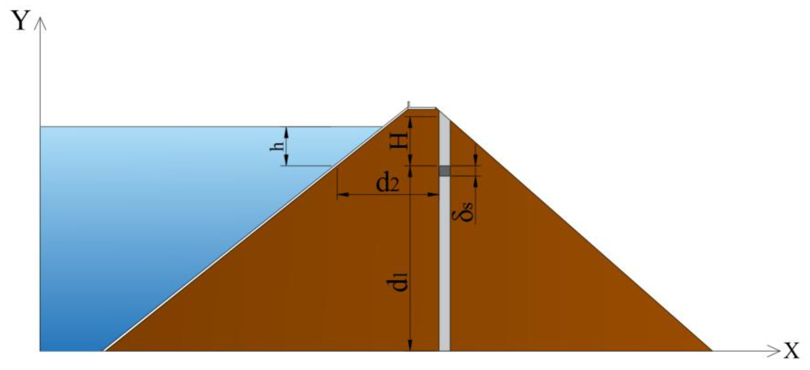
where b0, b1, b2 and b3 are the coefficients of regression; h is the elevation difference between the water level and the measuring point; d1 is the rockfill thickness; d2 is the distance from the measuring point to the face panel (Figure 1); represents the average water levels in the 3 days before the observation date; n is the modulus of elasticity index; and A is a constant.
2.1.2. The Temperature Component δS
The relationship between the deformation of rockfill body δS and temperature with the annual periodicity of the freezing period can be expressed by using the periodic function:
where t is the cumulative number of days from the monitoring date to the starting date.
2.1.3. The Time Effect Component δT
According to the monitoring data of the CFRD, the settlement in the late settlement period tends to converge gradually and eventually becomes stable. The settlement vs. per unit dam height (the proportion of settlement amount to dam height) has a linear relationship with the logarithm of time, as follows:
where α is the regression coefficient; H′ is the height of the dam; θ = t/100; θ0 = the cumulative number of days since the selected monitoring date/100; and n′ is the soil porosity at the measurement point.
2.1.4. The Rheological Component δε
The expression of the rheological component of the dam body should be combined with the rewritten formula of the vertical compression modulus [33] and the rheological curve, as shown below:
where a0 and a1 are the coefficients of regression; D is the initial relative deformation rate; γ is the bulk density of the filled rockfill; H is height of filled rockfill above the measuring point; Erc is the tangential modulus of the rockfill and according to the Duncan–Chang model; and Erc can be presented as:
where Rf is the failure ratio; σ1, σ3 are the large and small principal stresses, respectively; c is the cohesion force; φ is the friction angle; K is the tangent elastic modulus; and Pa is the atmospheric pressure.
Then, substituting Equation (6) into Equation (5), we can obtain the expression δε:
where n is the elastic modulus index; ξ is the lateral pressure coefficient, and
2.1.5. The Material Component δm
In this paper, three material parameters, namely, the soil porosity at the measurement point n′, the coefficient of compact permeability k, and the dry density ρ are brought into the regression analysis according to discrete variables. It is assumed that the functional relationship between a certain point settlement and its material parameters is as follows:
where f is the regression formula.
To sum up, the statistical model expression of the settlement of the rockfill during the operation period is established, which is the sum of the above components:
It should be noted that the temperature component is very small for the settlement of the mearing points, so it was not included in the final statistical model. According to the multi-factor MMP model, it can be found that the settlement deformation of the rockfill body is related to the three position factors of the upper fill elevation (H), the rockfill thickness (d1) and the distance from the measuring point to the face panel (d2). These three parameters can be used to represent the position coordinates of any point in the dam, so they can be used as variables to represent the spatial position. When the reservoir water level elevation is fixed, the deformation at different points is also related to the filling material at the location. These parameters are used to represent the comprehensive influence of the rockfill crushing characteristics, compression deformation properties or other factors in different rockfill areas, to explain the reasons for the differences in settlement values at different measuring points under the same external environmental conditions.
2.2. XGBoost Model for Multiple Monitoring Points Model
When the XGBoost prediction model of the MMP model for the settlement of CFRD is established, the input variables are 13 influence factors affecting the settlement, which are obtained from the statistical model (Equation (10)) of the running period of the rockfill. For the specific input variables, see Table 1. The output variable is the settlement value of 12 measuring points in the whole section. To show the superiority of the XGBoost model, we also perform the prediction using the base learner, which is a classification and regression tree (CART). A comparison between the performance of the XGBoost model and the CART model is shown to indicate the necessity of using the XGBoost model over simpler white box models.
2.3. Hyperparameter Optimization and Performance Measures
During model training, it is necessary to optimize the hyperparameters in the machine learning algorithm. Common hyperparameter optimization methods include grid search [29,34], random search, Bayesian optimization [35], etc. Grid search requires traversing all hyperparameter combinations, which consumes a lot of computational resources, which are already limited, and model training is slow. The random search method randomly selects different combinations of hyperparameters with great randomness. Bayesian optimization is a method of automatic adjustment of hyperparameters, which will track the evaluation results of every combination of hyperparameters tried in the past and form a probabilistic model. This model is called the “proxy” of the objective function. Before trying the next set of hyperparameters, the Bayesian optimization method will refer to this proxy model and select the hyperparameter with the best performance on the proxy function to evaluate the actual objective function. Compared with grid search and random search, Bayesian optimization has better performance and can reduce the computing time. In this paper, the method of Bayesian optimization combined with K-fold cross-validation is used to optimize the hyperparameters of the model. Using at the hyperparameter values selected by the Bayesian optimization algorithm, the K-fold cross-validation method was used to evaluate the performance of the model under the selected combination of hyperparameters. When the hyperparameters are optimized by Bayesian optimization, the domain space is the value range of the hyperparameter to be searched, and the objective function is the evaluation index value of the model’s prediction performance on the verification set using the current combination of hyperparameters. The specific steps are as follows:
(1) Establish the alternative probability model of the objective function: some hyperparameters are randomly generated in the domain space, and K-fold cross-validation is used to train and evaluate the model. The evaluation results are used to describe the ability b of these models and the prior data set O = {(a1, b1) …, (ak, bk)}. A Gaussian model, GM, is fitted based on O fitting. (2) Select the hyperparameter with the best performance on the agent function: find the maximum hyperparameter a′ under GM through the collection function. (3) Apply the selected optimal hyperparameter to the objective function: the model is trained and evaluated based on the hyperparameter a′ and K-fold cross-validation, and the evaluation results are used to describe the ability of the model b′. (4) Update the proxy model and add (a′, b′) to set O. (5) Repeat steps (2)~(4) until the maximum number of iterations or running time is reached.
The specific steps of K-fold cross-validation taken to train and evaluate the model are as follows: (1) Divide the training set into K parts. (2) i (i = 1, 2, …, K) is the test set, and the remaining K − 1 is the training set. K data sets are constructed. (3) For the current combination of hyperparameter values, K different models are trained based on the K data sets in step (2) and test index values are calculated. (4) Calculate the mean value of the K test index values as the evaluation value of the model’s prediction performance using the combination of corresponding hyperparameter values.
The XGBoost algorithm has many parameters, and different selections of parameter will affect the model’s prediction performance. The hyperparameters of the XGBoost model selected in this paper to be optimized and their implications are shown in Table 2, along with the range settings of each hyperparameter and the optimal value results under 5-fold cross-validation. The eta parameter is the shrinkage step size, and the model robustness can be improved by reducing the weight of each step. The value range is [0.01, 0.3]. Max_depth is the maximum depth of the decision tree. As the depth of the tree increases, the model will have a higher grasp of the local factors of the sample. The value range is [3, 10]. Learning_rate is the learning rate, which affects the speed at which the parameter is updated to the optimal value. The value range is [0.05, 0.3]. N is the maximum number of iterations or the maximum number of weak learners, which mainly affects the fitting degree of the model.
The mean absolute error (MAE), mean absolute percentage error (MAPE), root mean square error (RMSE) and coefficient of determination (R2) of different measurement points are used as quantitative indicators to evaluate the prediction ability of the model. The calculation of MAE, MAPE and RMSE and R2 are presented mathematically by Equations (12)–(14):
where y and the target and predicted values respectively, is the average of the target values and N is the number of data points.
2.4. Factor Importance Analysis Based on SHAP
The SHAP functions interpret the impact of each factor on the predicted value of each individual and provide the visible factor importance analysis [36,37]. It is an additive explanation model constructed by SHAP inspired by cooperative game theory with all the characteristics treated as “contributors” [38]. For each predicted sample, the model generates a predicted value, and the SHAP value is the value assigned to each factor in the sample [39]. The process of this analysis is as follows: Suppose that the ith sample is xi, the factor j of the ith sample is xij, m is the number of factors in the model, the predicted value of the sample is yi, the baseline of the whole model (usually the mean value of the target variable of all samples) is ybase, and the SHAP value is shown as follows [36]:
where f(xij) is the SHAP value of xi, e.g., f(xi1) is the contribution of the first factor in the ith sample to the final predicted value yi. When f(xi1) > 0, it indicates that this factor increases the predicted value, showing a positive correlation; otherwise, it indicates that this factor reduces the predicted value, which is a negative correlation. The new MMP model and the traditional model have 13 + 11 influencing factors, which are chosen as influencing factors (see Table 3). The factors of the new MMP model are represented by X series, while the factors of the traditional model are represented by Y series. It should be noted that all the factors are independent and have distinct meanings.
3. Case Study
We use the actual monitoring data of the Liyuan CFRD to evaluate the feasibility of settlement prediction using the newly derived MMP model. The Liyuan CFRD is located in the middle reach of the Jinsha River, Lijiang City, Yunnan Province. The dam began to be filled in the middle of August 2011, and the main part of the dam was completed at the end of July 2013. The construction period of the concrete panel was from 28 November 2013 to 28 May 2014, and the water storage began on 10 November 2014. The project’s reservoir has the capacity for cycle regulation, the normal water level is 1618 m, the dead water level is 1605 m, and the flood control limit water level is 1605 m (early July to early August). The maximum dam height of the Liyuan CFRD is 155 m, and the normal water storage capacity corresponds to 727 million m3.
We use the water level settlement gauge to monitor the settlement of the dam. The gauges were arranged along the river at a distance of 35 m to obtain the vertical displacement of the dam during the construction period and the operation period (see Figure 2). There are three monitoring points on the settlement’s maximum cross-section which are arranged horizontally along a straight line at the right side of the dam at 0 + 223 m. As shown in Figure 2, most of the measuring points are located in the main rockfill area, and some of them are located in the secondary rockfill area and the downstream rockfill area. The arrangement and range of 12 measuring points on the cross-section covers the whole section and can reflect the settlement of the whole rockfill dam under external load well, which is helpful in studying the prediction performance of the new MMP model. The monitoring data selected for modeling in this paper are from November 2014 to March 2016, that is, the period from the initial storage to the normal water level. The data were recorded once a week. A total of 924 effective data points can fully reflect the variation trend of the settlement at the initial stage of the storage operation.
4. Results
4.1. Prediction Accuracy of the New MMP Model
To verify the prediction accuracy and effectiveness of the new MMP model proposed in this paper, a full-section deformation prediction model is established for the settlement of the Liyuan CFRD measured at 12 monitoring points. We select 77 sets of settlement data from the initial impounding in November 2014 to the normal water level in March 2016 as samples for the analysis. A total of 924 valid data from 12 measurement points can fully reflect the variation trend of the initial impounding settlement. The first 67 groups are used as training data, and the last 10 groups are used as test data. The prediction period is from July 2015 to March 2016. The period is 8 months. The long-period test set is helpful to evaluate the prediction performance of the new MMP model.
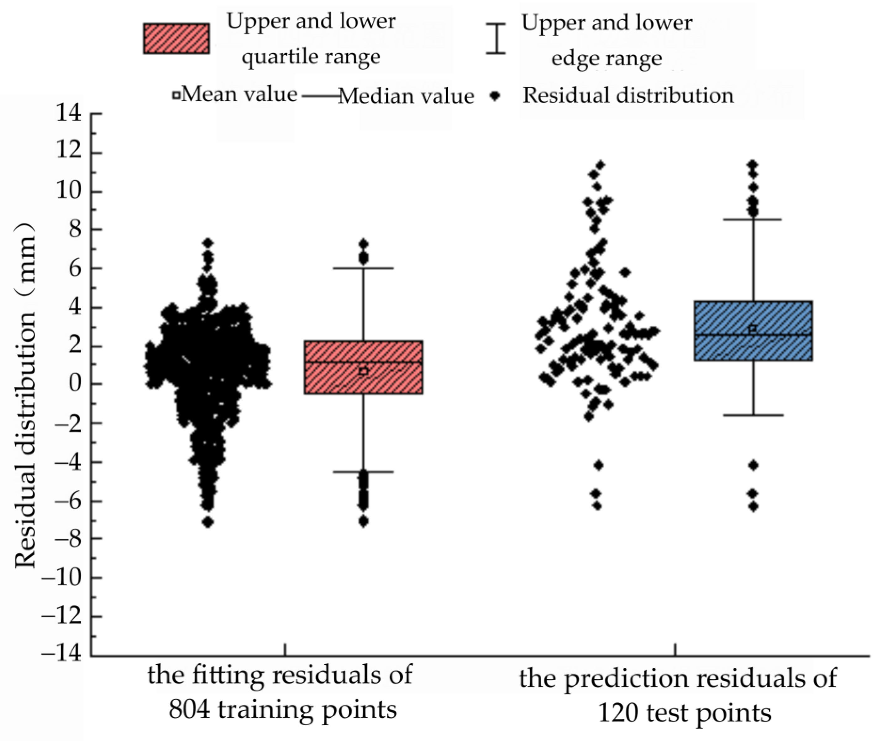
The predicted residual distribution of the new MMP model is shown in Figure 3. As can be seen from Figure 3 and Table 4, the normal distribution of the fitting residuals of the 804 training groups used in the XGBoost model is mainly between −1 mm and 2 mm; the mean and median of the residuals in the training set are about 1 mm, while the MAE and RMSE values of each measurement point in the training set are mostly in the fitting error range of 0–3 mm. The results show that the new MMP model can fit the deformation of measuring points in the same section well. In the test set, the mean and median of the residuals of 120 groups were slightly higher than 2 mm, and the prediction errors of each measurement point were also around 2–3 mm. The difference between the fitting and predicted residual values were small, indicating that the overall performance of the XGBoost model was precise and had a good prediction performance.
We then compared the subsidence obtained from XGBoost model and the CART model. The prediction accuracy of the two algorithms (XGBoost and CART) can be quantitatively compared using the data in Table 4. R2 is used to measure the correlation between the actual value and the predicted value. The larger R2 is, the more accurate the prediction of the algorithm is. In the test set, only the R2 of XGBoost algorithm is above 0.90, larger than that of the CART model (around 0.6). This phenomenon shows that the XGBoost algorithm has a higher prediction accuracy than its base algorithm (CART). The RMSE, MAE and MAPE are all used to measure the difference between the actual value and the predicted value. It can be seen that the model’s MAE and RMSE values at each measurement point in the training set and the test set are smaller than 3 mm, while the RMSE and MAPE of the test set from the CART algorithms are above 3 mm. The MAPE values of the training set and test set from the XGBoost algorithm are less than 1%, much smaller than those from the CART algorithm, which are mostly higher than 1%. It can be seen that for predicting the settlement of the CFRD, the predicted value of XGBoost shows the best correlation with the actual value and the smallest error. This finding demonstrates the superiority of the XGBoost model and indicates the importance of the use of the XGBoost algorithm.
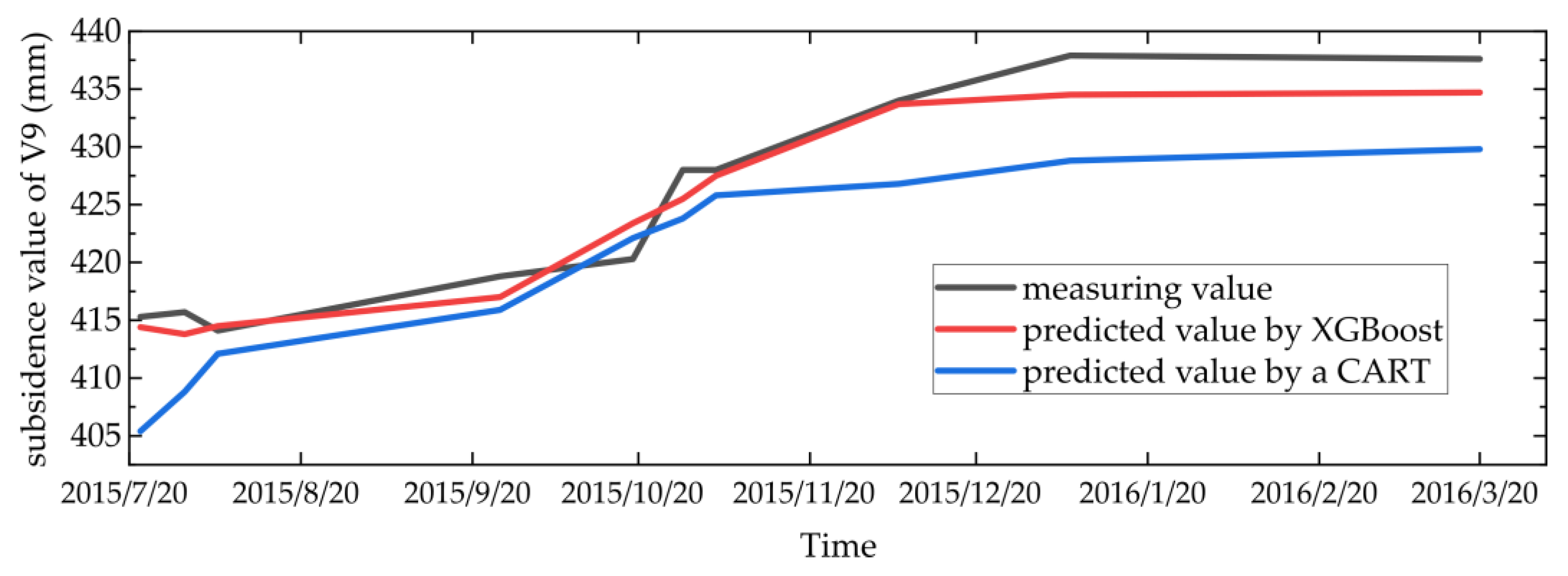
We also provide a scatter plot of the predicted and actual response values of one typical monitoring point, V9, in Figure 4. The figure shows that the predicted values of the settlement of the measuring point continuously increase. This trend is the same for the measuring value. Furthermore, the prediction accuracy of the XGBoost model is higher than the CART model. This result is consistent with the MAE, RMSE and MAPE values.
All in all, the new MMP model has the best prediction accuracy for measuring points V9-V10 in the maximum settlement area, and the MAE and RMSE values of the three measuring points are all about 2 mm. The prediction errors of most measuring points are within 1.5–3 mm, and the MAPE is also lower than 1%, indicating that the new MMP model had a good performance in predicting global measuring points. Moreover, the stability of the model also needs to be assessed in future works.
4.2. Orders of Importance of Factors by SHAP
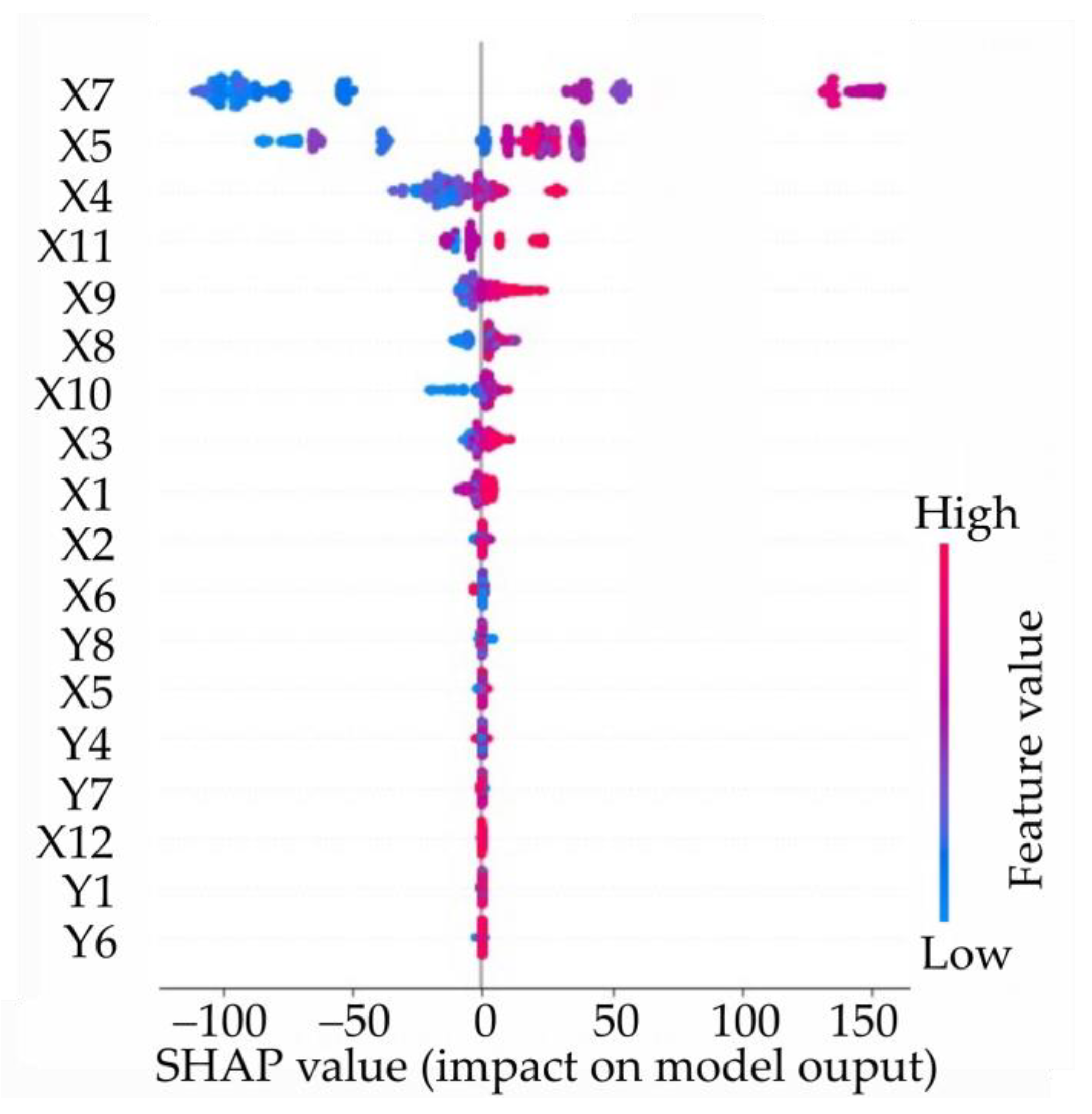
Figure 5 shows the evaluation results of characteristic values of factors obtained by the SHAP method. Each row in Figure 5 represents a factor, each point represents a monitoring sample, and the x-axis represents the SHAP value. A redder color represents a larger value of the impact factor, and a bluer color represents the smaller the value of the impact factor itself. It can be seen that the orders of importance of factors of the new MMP point model are generally higher than those of the traditional model, except for the coordinate Y8. This finding indicates that the new MMP model is more suitable for predicting the settlement of CFRDs. It can be intuitively seen from the evaluation results that the newly added spatial location components X7, X5 and X4 are important contribution factors of the model, and they are all coupling factors related to the upper fill elevation. In addition, the upper fill elevation (H) is the most important characteristic factor. The rheological component X4, which includes the upper fill elevation, makes a great contribution to the model. The new spatial location also has higher contribution and adaptability than x and y in the traditional model, indicating that the position component derived from the new MMP model is more advantageous. Furthermore, points X4 and X8 gradually turn red with the increase in the SHAP value, indicating that these factors have a positive relationship with the settlement. In another word, the increase in the upper fill elevation value leads to an increase in settlement value. The upper fill elevation (X7) and the distance from the measuring point to the panel (X5) are also positively correlated with the settlement. Interestingly, median values of features X7 and X5 (represented by a purple color in Figure 5) can have the maximum contribution value to the settlement. Combined with the characteristic distribution of the spatial location parameters, the training characteristics of the MMP model can be roughly inferred, that is, the settlement at the top of the dam and at its foundation is small, the settlement at downstream of the dam body is larger, the maximum settlement is about half of the dam body’s elevation, the settlement at the downstream rockfill area is slightly larger than that at the upstream side and the predicted value is basically consistent with the actual deformation.
From Figure 5, we can further analyze the orders of importance of the water level, time and temperature components. In the water level component, the significance of X1 (which represents the transfer effect of water pressure) is higher than that of traditional water pressure Y1. This indicates that the combination of water pressure and spatial position can effectively improve the settlement. At the same time, the importance of X1 is also higher than the mean water level pressure X2 and the rheology–water pressure component X3, which proves that the hydrostatic load is the main factor of the settlement. Both X9 and X10 rank high because the time component is used to characterize the irreversible sedimentation over time. The least important component is the temperature component, as it is shown that Y4–Y7 have little influence on settlement, which basically conforms to the actual situation that the deformation of the CFRD has little correlation with periodic changes in temperature.
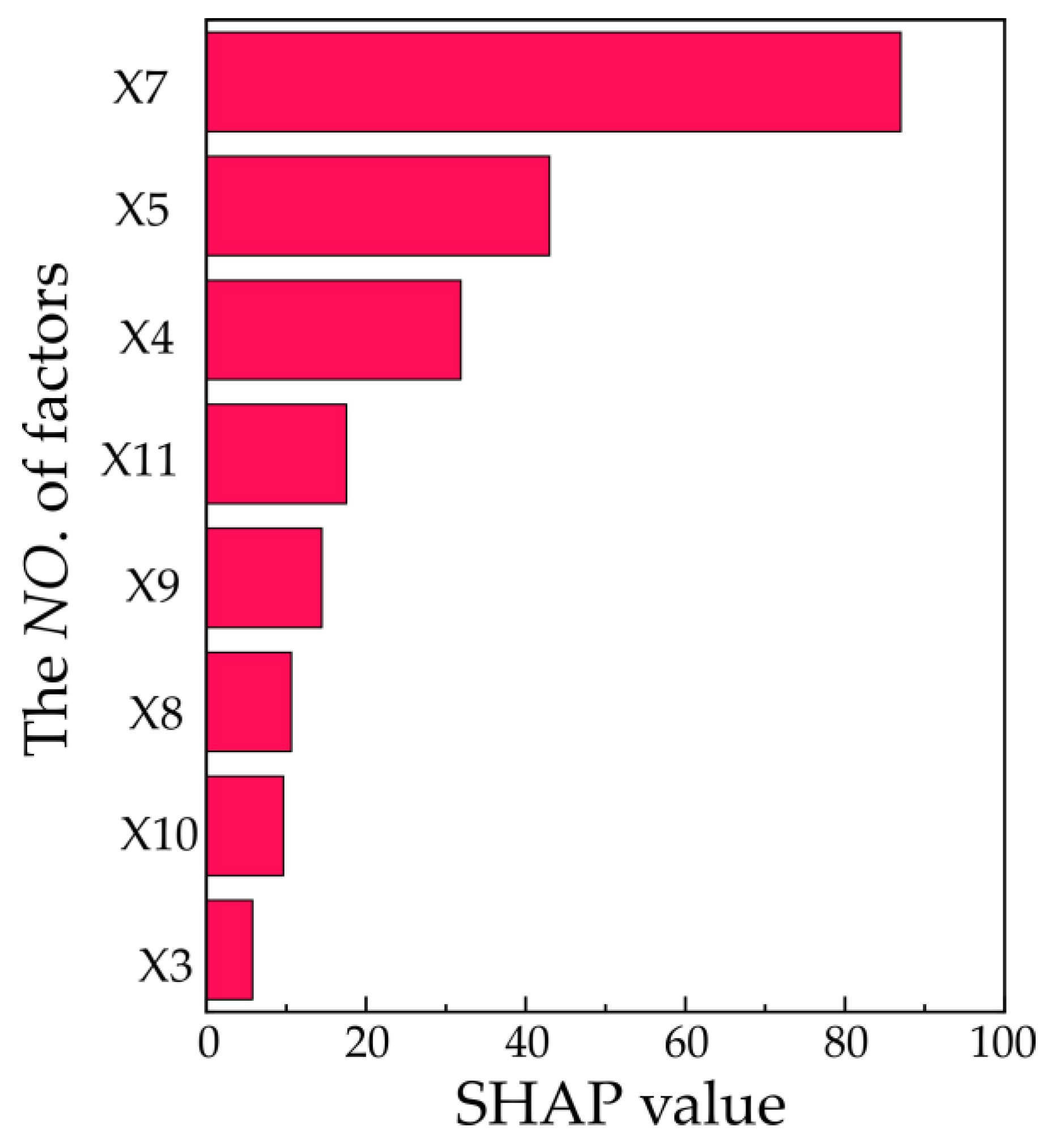
We further present the mean of the absolute SHAP values for each factor across the whole dataset in Figure 6. We only present several important factors; the other factors that have very low SHAP values are not present. The results show that in the MMP model, the contribution of the factors related to the spatial location (X7 and X5) to the settlement is the largest, while the contributions of the three traditional BP components of water level (X3), time and temperature (X9, X10 and other factors not shown in Figure 6), which represent temporal changes, are somewhat weaker. As a sum of a spatial model and a temporal model, the settlement of the measuring point consists of the completed settlement reference value in the filling period and the temporal value in the operating period. The spatial location component (X7 and X5) and material component (X11) determine the basic settlement, while the water level (X3) and time component (X9 and X10) affect the temporal variation in the settlement. Compared with the time series value with a smaller variation range, the basic settlement at the measuring point accounts for the main part of the settlement value, often reaching more than 80% of the total settlement. Therefore, in the monitoring data set of the full-section measuring points during the study of the water storage operation period, the spatial component (X7 and X5) and the material component have the largest average SHAP values contributing to the settlement. Moreover, their contribution is greater than that of the temporal component (X9 and X10), which also confirms the prediction accuracy of the MMP model. Furthermore, it is validated that it is necessary to pay attention to the spatially related variables in the study of the overall dam deformation.
Two typical single prediction plots using the XGBoost model are shown in Figure 7. The length and color of the bars in Figure 7 show the degree of significance and direction (negative or positive) of the effect of each factor, respectively. The base value denotes the average of the observed response values. The prediction of point V9 on 30 March 2016 is shown in Figure 7a. The upper fill elevation H (X7) showed the highest effect, followed by the distance from the measuring point to the panel d (X5). Their values are lower than the median, and they both have a negative effect on the settlement. This phenomenon is same with the global SHAP value shown in Figure 5, where the points of X7 and X5 are in blue and often have a negative SHAP value and thus have a negative effect on the subsidence. What is more, X9 has the largest positive effect on the subsidence for V9. This is because X9 is related to the monitoring days and has the largest value. The prediction of point V10 on 30 March 2016 is shown in Figure 7b. All factors in Figure 7b show positive influences. V10 is located in the middle part of the CFRD, and has the largest settlement. Among these factors, the upper fill elevation H (X7) showed the highest effect. The distance from the measuring point to the panel d1 (X5) ranks second. This phenomenon is the same with V9. However, although X5 has a median value, it has the highest SHAP value; this corresponds to the purple dots of X5 in the large SHAP value areas in Figure 5. Based on the individual analysis of the MMP model, the prediction process and prediction basis of the model for each specific sample can be understood. According to the data, the point position has the largest impact on the subsidence, and the monitoring time also has significant effects.
To sum up, from the feature importance analysis, it can be seen that the contribution of the influence factors of the newly derived MMP model is better than that of the traditional variables. The average SHAP value of the spatial component and the material component to the output settlement is the largest, and the factor contribution is greater than that of the temporal correlation component, which confirms that the prediction accuracy of the MMP model is closely related to the spatial location component. In the study of the overall deformation behavior of a CFRD, it is necessary to pay attention to the spatially related variables.
5. Conclusions
The MMP prediction model is based on the physical cause analysis of a CFRD settlement and the expansion of spatial components. The influence of water level load transfer, rockfill rheology and soil properties on the settlement during the operation period of impoundment is comprehensively analyzed, and a space-time distribution model of the CFRD during the operation period under the action of multiple factors is established. The XGBoost model was used for fitting prediction, and the model was evaluated by various performance indicators. Taking the settlement monitoring data of the Liyuan CFRD as an example, the new MMP model, under the action of multiple factors, can predict the settlement of full section points with higher accuracy, which has certain application and popularization value for related projects. From the factor importance analysis, it can be confirmed that the contribution of the influencing variables of the MMP model to the model is better than that of the traditional variables. The SHAP value of the spatial component and the material component to the output settlement value is the largest, and the factor contribution is greater than that of the time component, which confirms that the prediction accuracy of the MMP model is closely related to the spatial location component. In the study of the overall deformation behavior of CFRD, it is necessary to pay attention to the spatially related variables. Our work elucidates the high prediction accuracy of the newly established MMP model and provides a benchmark for the investigation of the safety management of a CFRD over its whole life cycle. Practitioners can predict future dam deformation based on dam deformation data, obtain the dominant factors and repair them in advance. However, this MMP and XGBoost model has only been validated on one CFRD, more data from other CFRDs are needed to test the MMP and XGBoost model. In addition, this new model was developed from the physical analysis of a CFRD, and whether or not it is suited for other dams also needs to be investigated in future work.
Author Contributions
Conceptualization, T.W.; Methodology, Z.W.; Software, Y.W.; Validation, Z.W.; Formal analysis, K.M.; Investigation, Y.W.; Writing—original draft, L.S.; Writing—review and editing, T.W.; Supervision, T.W. All authors have read and agreed to the published version of the manuscript.
Funding
This research was funded by the National Natural Science Foundation of China [52079109].
Data Availability Statement
Not applicable.
Conflicts of Interest
The authors declare no conflict of interest.
References
- Tatin, M.; Briffaut, M.; Dufour, F.; Simon, A.; Fabre, J.-P. Thermal displacements of concrete dams: Accounting for water temperature in statistical models. Eng. Struct. 2015, 91, 26–39. [Google Scholar] [CrossRef]
- Hu, Y.; Shao, C.; Gu, C.; Meng, Z. Concrete Dam Displacement Prediction Based on an ISODATA-GMM Clustering and Random Coefficient Model. Water 2019, 11, 714. [Google Scholar] [CrossRef] [Green Version]
- Min, K.; Li, Y.; Yin, Q.; Wen, L. Research on prediction performance of multiple monitoring points model based on support vector machine. IOP Conf. Ser. Mater. Sci. Eng. 2020, 794, 012038. [Google Scholar] [CrossRef]
- He, J.-P.; Tu, Y.-Y.; Shi, Y.-Q. Fusion Model of Multi Monitoring Points on Dam Based on Bayes Theory. Procedia Eng. 2011, 15, 2133–2138. [Google Scholar] [CrossRef] [Green Version]
- Cheng, L.; Zheng, D. Two online dam safety monitoring models based on the process of extracting environmental effect. Adv. Eng. Softw. 2013, 57, 48–56. [Google Scholar] [CrossRef]
- Salazar, F.; Morán, R.; Toledo, M.Á.; Oñate, E. Data-Based Models for the Prediction of Dam Behaviour: A Review and Some Methodological Considerations. Arch. Comput. Methods Eng. 2017, 24, 1–21. [Google Scholar] [CrossRef] [Green Version]
- Arlot, S.; Celisse, A. A survey of cross-validation procedures for model selection. Statist. Surv. 2010, 4, 40–79. [Google Scholar] [CrossRef]
- Sun, X.; Zheng, D.; Zhou, M. Spatiotemporal Prediction Model for Settlement Value of Face Rockfill Dam During Operation Period. J. China Three Gorges Univ. Nat. Sci. 2019, 41, 5–8. [Google Scholar]
- Huang, D.; Liu, B.; Dai, W. Building multiple-point displacement model of Wuqiangxi dam based on BP neural network. Geotech. Investig. Surv. 2017, 45, 62–64. [Google Scholar]
- Chai, L.; Qi, D.; Wu, H. Application of multi-point and multidirectional BP Network Model in Dam deformation monitoring. Water Resour. Power 2014, 32, 94–97. [Google Scholar]
- Li, Y.; Min, K.; Zhang, Y.; Wen, L. Prediction of the failure point settlement in rockfill dams based on spatial-temporal data and multiple-monitoring-point models. Eng. Struct. 2021, 243, 112658. [Google Scholar] [CrossRef]
- Lu, X.; Wu, Z.; Zhou, Z.; Chen, J. Research on the Prediction Model of Deformation of High Core Rockfill Dam During Construction Period. Adv. Eng. Sci. 2017, 49, 61–69. [Google Scholar] [CrossRef]
- Kang, F.; Liu, J.; Li, J.; Li, S. Concrete dam deformation prediction model for health monitoring based on extreme learning machine. Struct. Control Health Monit. 2017, 24, e1997. [Google Scholar] [CrossRef]
- Wei, B.; Yuan, D.; Xu, Z.; Li, L. Modified hybrid forecast model considering chaotic residual errors for dam deformation. Struct. Control Health Monit. 2018, 25, e2188. [Google Scholar] [CrossRef]
- Taffese, W.Z.; Sistonen, E. Machine learning for durability and service-life assessment of reinforced concrete structures: Recent advances and future directions. Autom. Constr. 2017, 77, 1–14. [Google Scholar] [CrossRef]
- McCulloch, W.S.; Pitts, W. A logical calculus of the ideas immanent in nervous activity. Bull. Math. Biophys. 1943, 5, 115–133. [Google Scholar] [CrossRef]
- Kim, Y.-S.; Kim, B.-T. Prediction of relative crest settlement of concrete-faced rockfill dams analyzed using an artificial neural network model. Comput. Geotech. 2008, 35, 313–322. [Google Scholar] [CrossRef]
- Su, H.; Chen, Z.; Wen, Z. Performance improvement method of support vector machine-based model monitoring dam safety: Performance Improvement Method of Monitoring Model of Dam Safety. Struct. Control Health Monit. 2016, 23, 252–266. [Google Scholar] [CrossRef]
- Marandi, S.M.; VaeziNejad, S.M.; Khavari, E. Prediction of Concrete Faced Rock Fill Dams Settlements Using Genetic Programming Algorithm. IJG 2012, 3, 601–609. [Google Scholar] [CrossRef] [Green Version]
- Chen, T.; Guestrin, C. Xgboost: A scalable tree boosting system. In Proceedings of the 22nd ACM SIGKDD International Conference on Knowledge Discovery and Data Mining, San Francisco, CA, USA, 13–17 August 2016; pp. 785–794. [Google Scholar]
- Nguyen, L.T.K.; Chung, H.-H.; Tuliao, K.V.; Lin, T.M.Y. Using XGBoost and Skip-Gram Model to Predict Online Review Popularity. SAGE Open 2020, 10, 215824402098331. [Google Scholar] [CrossRef]
- Lim, S.; Chi, S. Xgboost application on bridge management systems for proactive damage estimation. Adv. Eng. Inform. 2019, 41, 100922. [Google Scholar] [CrossRef]
- Shi, N.; Li, Y.; Wen, L.; Zhang, Y. Rapid prediction of landslide dam stability considering the missing data using XGBoost algorithm. Landslides 2022, 19, 2951–2963. [Google Scholar] [CrossRef]
- Wakjira, T.G.; Rahmzadeh, A.; Alam, M.S.; Tremblay, R. Explainable machine learning based efficient prediction tool for lateral cyclic response of post-tensioned base rocking steel bridge piers. Structures 2022, 44, 947–964. [Google Scholar] [CrossRef]
- Wakjira, T.G.; Ibrahim, M.; Ebead, U.; Alam, M.S. Explainable machine learning model and reliability analysis for flexural capacity prediction of RC beams strengthened in flexure with FRCM. Eng. Struct. 2022, 255, 113903. [Google Scholar] [CrossRef]
- Nguyen, H.D.; Truong, G.T.; Shin, M. Development of extreme gradient boosting model for prediction of punching shear resistance of r/c interior slabs. Eng. Struct. 2021, 235, 112067. [Google Scholar] [CrossRef]
- Wang, L.; Wu, C.; Tang, L.; Zhang, W.; Lacasse, S.; Liu, H.; Gao, L. Efficient reliability analysis of earth dam slope stability using extreme gradient boosting method. Acta Geotech. 2020, 15, 3135–3150. [Google Scholar] [CrossRef]
- Wakjira, T.G.; Ebead, U.; Alam, M.S. Machine learning-based shear capacity prediction and reliability analysis of shear-critical RC beams strengthened with inorganic composites. Case Stud. Constr. Mater. 2022, 16, e01008. [Google Scholar] [CrossRef]
- Wakjira, T.G.; Abushanab, A.; Ebead, U.; Alnahhal, W. FAI: Fast, accurate, and intelligent approach and prediction tool for flexural capacity of FRP-RC beams based on super-learner machine learning model. Mater. Today Commun. 2022, 33, 104461. [Google Scholar] [CrossRef]
- AlKhereibi, A.H.; Wakjira, T.G.; Kucukvar, M.; Onat, N.C. Predictive Machine Learning Algorithms for Metro Ridership Based on Urban Land Use Policies in Support of Transit-Oriented Development. Sustainability 2023, 15, 1718. [Google Scholar] [CrossRef]
- Al-Hamrani, A.; Wakjira, T.G.; Alnahhal, W.; Ebead, U. Sensitivity analysis and genetic algorithm-based shear capacity model for basalt FRC one-way slabs reinforced with BFRP bars. Compos. Struct. 2023, 305, 116473. [Google Scholar] [CrossRef]
- Ishfaque, M.; Salman, S.; Jadoon, K.Z.; Danish, A.A.K.; Bangash, K.U.; Qianwei, D. Understanding the Effect of Hydro-Climatological Parameters on Dam Seepage Using Shapley Additive Explanation (SHAP): A Case Study of Earth-Fill Tarbela Dam, Pakistan. Water 2022, 14, 2598. [Google Scholar] [CrossRef]
- Sigtryggsdóttir, F.G.; Snæbjörnsson, J.T.; Grande, L. Statistical Model for Dam-Settlement Prediction and Structural-Health Assessment. J. Geotech. Geoenviron. Eng. 2018, 144, 04018059. [Google Scholar] [CrossRef]
- Liashchynskyi, P.; Liashchynskyi, P. Grid search, random search, genetic algorithm: A big comparison for NAS. arXiv 2019, arXiv:1912.06059. [Google Scholar]
- Snoek, J.; Larochelle, H.; Adams, R.P. Practical bayesian optimization of machine learning algorithms. Adv. Neural Inf. Process. Syst. 2012, 25, 2960–2968. [Google Scholar]
- Dong, W.; Huang, Y.; Lehane, B.; Ma, G. An artificial intelligence-based conductivity prediction and feature analysis of carbon fiber reinforced cementitious composite for non-destructive structural health monitoring. Eng. Struct. 2022, 266, 114578. [Google Scholar] [CrossRef]
- Panda, C.; Mishra, A.K.; Dash, A.K.; Nawab, H. Predicting and explaining severity of road accident using artificial intelligence techniques, SHAP and feature analysis. Int. J. Crashworthiness 2022. [Google Scholar] [CrossRef]
- Štrumbelj, E.; Kononenko, I. Explaining prediction models and individual predictions with feature contributions. Knowl. Inf. Syst. 2014, 41, 647–665. [Google Scholar] [CrossRef]
- Shapley, L.S. A Value for N-Person Games. In Classics in Game Theory; Princeton University Press: Princeton, NJ, USA, 1997; Volume 69. [Google Scholar]
Figure 1.
Schematic diagram of monitoring point affected by rheology and soil weight.

Figure 2.
The layout of monitoring points of Liyuan dam.

Figure 3.
Box chart of model fitting and prediction residuals.

Figure 4.
Predicted values and monitoring values of monitoring point V9 using different algorithms.

Figure 5.
Evaluation results of factor values based on SHAP. A redder color represents a larger impact factor, and a bluer color is a smaller impact factor.
Figure 5.
Evaluation results of factor values based on SHAP. A redder color represents a larger impact factor, and a bluer color is a smaller impact factor.

Figure 6.
The mean of the absolute SHAP values for each factor across the whole dataset.

Figure 7.
Evaluation results of factors based on SHAP values. (a) The prediction of point V9 on 30 March 2016; (b) The prediction of point V10 on 30 March 2016. A redder color represents a larger impact factor, and a bluer color represents a smaller impact factor.
Figure 7.
Evaluation results of factors based on SHAP values. (a) The prediction of point V9 on 30 March 2016; (b) The prediction of point V10 on 30 March 2016. A redder color represents a larger impact factor, and a bluer color represents a smaller impact factor.


Table 1.
Input variable set.
| Water Level Component (δH) | Rheology–Soil Weight Component (δε) | Time Effect Component (δT) | Material Component (δm) | |
|---|---|---|---|---|
| Factors |
Table 2.
Parameters of XGBoost Model.
| Parameters | Value | Range | Note |
|---|---|---|---|
| eta | 0.2 | [0.01, 0.3] | the shrinkage step size |
| max_depth | 5 | [3, 10] | the maximum depth of the decision tree |
| learning_rate | 0.1 | [0.05, 0.3] | the learning rate |
| N | 160 | / | the maximum number of iterations |
Table 3.
Influence variables set.
| Components from the MMP Model | NO. | Factors | Components from the Traditional Model | NO. | Factors |
|---|---|---|---|---|---|
| Water level component | X1 | Water level component | Y1 | ||
| X2 | Y2 | ||||
| X3 | Y3 | ||||
| Rheology–soil weight component | X4 | Temperaturecomponent | Y4 | ||
| X5 | Y5 | ||||
| X6 | Y6 | ||||
| X7 | Y7 | ||||
| X8 | Location component | Y8 | |||
| Time effect component | X9 | Y9 | |||
| X10 | Time effect component | Y10 | |||
| Material component | X11 | Y11 | |||
| X12 | Note: Time effect components are same in the two models; X5(d2) and Y9(y) are the same. | ||||
| X13 | r | ||||
Table 4.
Settlement fitting and prediction performance analysis of new multiple points monitoring model.
Table 4.
Settlement fitting and prediction performance analysis of new multiple points monitoring model.
| Measuring Point | Training Set | Test Set by XGboost | Test Set by CART | |||||||||
|---|---|---|---|---|---|---|---|---|---|---|---|---|
| MAE /mm | RMSE /mm | MAPE/% | R2 | MAE /mm | RMSE /mm | MAPE/% | R2 | MAE /mm | RMSE /mm | MAPE/% | R2 | |
| V2 | 3.41 | 4.18 | 1.54 | 0.88 | 7.31 | 7.74 | 2.65 | 0.85 | 9.54 | 8.65 | 5.88 | 0.49 |
| V3 | 1.34 | 1.57 | 0.34 | 0.97 | 1.95 | 2.18 | 0.47 | 0.94 | 6.87 | 8.64 | 3.76 | 0.56 |
| V4 | 2.24 | 2.58 | 0.54 | 0.95 | 4.00 | 4.19 | 0.88 | 0.93 | 5.88 | 6.00 | 1.56 | 0.58 |
| V5 | 1.49 | 1.92 | 0.24 | 0.98 | 3.17 | 3.54 | 0.50 | 0.92 | 4.67 | 4.99 | 1.09 | 0.58 |
| V6 | 0.93 | 1.37 | 0.17 | 0.99 | 1.35 | 2.05 | 0.24 | 0.96 | 4.56 | 3.77 | 1.88 | 0.64 |
| V7 | 1.27 | 2.02 | 0.39 | 0.94 | 1.97 | 2.49 | 0.55 | 0.92 | 3.64 | 5.85 | 1.55 | 0.56 |
| V9 | 2.39 | 2.86 | 0.62 | 0.95 | 1.77 | 2.09 | 0.41 | 0.93 | 5.47 | 6.16 | 1.2 | 0.59 |
| V10 | 1.80 | 2.23 | 0.26 | 0.98 | 1.67 | 2.23 | 0.24 | 0.95 | 2.67 | 4.73 | 0.89 | 0.65 |
| V11 | 2.44 | 2.68 | 0.49 | 0.96 | 2.14 | 2.48 | 0.42 | 0.93 | 4.34 | 4.53 | 1.14 | 0.67 |
| V12 | 0.68 | 2.04 | 0.22 | 0.97 | 1.22 | 3.15 | 0.34 | 0.94 | 1.54 | 3.86 | 0.39 | 0.73 |
| V14 | 1.23 | 2.22 | 0.34 | 0.94 | 4.12 | 4.79 | 1.00 | 0.90 | 8.12 | 8.42 | 3.55 | 0.62 |
| V15 | 0.61 | 2.46 | 0.23 | 0.95 | 7.08 | 7.55 | 2.03 | 0.85 | 10.57 | 10.05 | 7.89 | 0.50 |
Disclaimer/Publisher’s Note: The statements, opinions and data contained in all publications are solely those of the individual author(s) and contributor(s) and not of MDPI and/or the editor(s). MDPI and/or the editor(s) disclaim responsibility for any injury to people or property resulting from any ideas, methods, instructions or products referred to in the content. |
© 2023 by the authors. Licensee MDPI, Basel, Switzerland. This article is an open access article distributed under the terms and conditions of the Creative Commons Attribution (CC BY) license (https://creativecommons.org/licenses/by/4.0/).
Share and Cite
MDPI and ACS Style
Shao, L.; Wang, T.; Wang, Y.; Wang, Z.; Min, K. A Prediction Model and Factor Importance Analysis of Multiple Measuring Points for Concrete Face Rockfill Dam during the Operation Period. Water 2023, 15, 1081. https://doi.org/10.3390/w15061081
AMA Style
Shao L, Wang T, Wang Y, Wang Z, Min K. A Prediction Model and Factor Importance Analysis of Multiple Measuring Points for Concrete Face Rockfill Dam during the Operation Period. Water. 2023; 15(6):1081. https://doi.org/10.3390/w15061081
Chicago/Turabian StyleShao, Lei, Ting Wang, Youde Wang, Zilong Wang, and Kaiyi Min. 2023. "A Prediction Model and Factor Importance Analysis of Multiple Measuring Points for Concrete Face Rockfill Dam during the Operation Period" Water 15, no. 6: 1081. https://doi.org/10.3390/w15061081
Note that from the first issue of 2016, this journal uses article numbers instead of page numbers. See further details here.