Water Pipeline Leak Detection Based on a Pseudo-Siamese Convolutional Neural Network: Integrating Handcrafted Features and Deep Representations

Abstract

The detection of leaks in water distribution systems (WDS) has always been a major concern for urban water supply companies. However, the performance of traditional leak detection classifiers highly depends on the effectiveness of handcrafted features. An alternative method is to use a convolutional neural network (CNN) to process raw signals directly to obtain deep representations that may ignore prior information about the leakage. The study proposes a novel approach to leak detection in WDS using ground acoustic signals, and demonstrates the effectiveness of combining handcrafted features and deep representations using a pseudo-siamese convolutional neural network (PCNN) model. Mel frequency cepstral coefficient (MFCCs) are selected as additional handcrafted features to traditional time- and frequency-domain (TFD) features. Based on the results of the model performance evaluation, the optimized PCNN model performs better than other methods, with an accuracy of 99.70%. A quantitative analysis of the PCNN demonstrates the effectiveness of handcrafted features and deep representations. Model visualization and interpretation analysis show that feature fusion occurs in the feedforward of the PCNN, hence improving the model’s performance. The present work can effectively support the development of novel intelligent leak detection equipment for WDS.

1. Introduction

Leaks in water distribution systems (WDS) can cause huge economic losses for water supply companies as well as a massive waste of water resources and environmental risks [1]. To detect and identify leaks, several leak detection methods have been proposed in previous studies [2,3,4,5]. Among these methods, acoustic leak detection technology, especially non-destructive acoustic leak detection technology, has gained considerable attention due to its high efficiency and accuracy [6]. Traditional acoustic leak detection surveys using listening devices (for example, listening rods and ground microphones) have been proven to be reliable. However, this method is labor-intensive and highly dependent on the experience of the user [7]. The most rapidly developing acoustic method is correlation analysis, which is more efficient than traditional acoustic detection methods [6]. However, it has some limitations. For example, correlation analysis methods are very effective when applied to metal pipes, but when applied to plastic pipes, they still face challenges due to the high attenuation of plastic pipes [8]. Using listening devices is an effective non-intrusive leak detection method that is insensitive to the material of the pipe. Although this method has some subjectivity, it is becoming increasingly important as more and more plastic pipes are used for water supply. It has been reported that plastic pipes account for 85% of water supply pipes below DN400mm in China [9]. It can be inferred that using listening devices with automatic leak detection algorithms can significantly improve their performance and reduce their dependence on intensive labor. Thus, it is essential to devise automatic leak detection algorithms and architectures that are both highly precise and adaptable, utilizing acoustic signals for effective leak detection.

To achieve automatic leak detection for WDS, several data-driven leak detection systems and methods have been developed by combining handcrafted features with supervised learning algorithms [10,11,12,13,14,15]. The performance of traditional supervised learning algorithms heavily relies on the effectiveness of handcrafted features, making feature extraction an essential part of classification systems. In previous studies [16,17], time- and frequency-domain (TFD) features were the most common handcrafted features for leak identification. In addition to TFD features, other handcrafted features based on different principles (such as Itakura distance [15] and damage sensitive features [12]) have also achieved satisfactory performance. Despite the effectiveness of handcrafted-feature-based (HFB) classifiers for leak detection, the method has some drawbacks. First, the selected handcrafted features may contain distortions or unnecessary information that may cause overfitting and decrease the computational efficiency of the classifier. Another drawback is that the selected handcrafted features may not necessarily be the most suitable for a specific domain [18]. In addition, the performance of certain handcrafted features is limited by prevailing scenarios. False alarms always happen when environmental noise has similar time and frequency characteristics to leak signals [19]. The solution to these problems involves extracting and selecting more powerful features, feature engineering (for example, principal component analysis [20]), and additional signal processing [21,22] of the raw signals.

Recent years have seen a growing interest in using the convolutional neural network (CNN) to automatically extract features (that is, deep representations) from acoustic signals and detect leaks in pressurized pipelines [18,23,24,25,26,27,28]. Contrary to traditional HFB supervised learning algorithms [16], CNN can automatically extract an optimal deep representation of data from raw signals without prior feature selection, hence making the process more objective and less biased [29]. To identify leaks in water supply pipelines, Kang et al. [18] proposed an ensemble CNN-SVM model based on one-dimension acoustic signals, and demonstrated that the performance of the model was better than that of some HFB classifiers. Similarly, studies [23,24] have employed time-frequency analysis to convert one-dimensional raw signals into two-dimensional spectrograms and proposed CNNs with different structures that successfully identified leaks in WDS. Research has shown that CNNs can automatically extract useful features from input signals for distinguishing leak signals and non-leak signals. However, CNNs may not always provide the most effective features when the features are extracted automatically, due to the extensive hyperparameters needing optimization.

Despite the effectiveness of CNNs, studies have shown that CNNs cannot completely outperform HFB classifiers in some fields [30,31,32]. According to these studies, handcrafted features are likely to be more generalizable in specific domains. In the field of leak detection, there is also some evidence that shows deep representations and handcrafted features have some complementarity [18]. However, the majority of current research in automatic leak detection in WDS focused on the optimization of CNN structures and their application to specific scenarios. To some extent, utilizing CNN directly to extract features from raw signals discards the prior knowledge about leakage derived from traditional signal analysis methods. It can be inferred that selecting appropriate handcrafted features and combining them with deep representations may be a better approach for leak detection in WDS. To address this issue, a pseudo-siamese convolutional neural network [33] (PCNN) model for feature fusion is utilized in this study. The PCNN is based on neural networks composed of two or more independent convolutional streams which process different inputs simultaneously. The perception design of the PCNN is flexible, and the known information can be fully utilized [34]. The concept of PCNN has been applied in numerous fields, including spatiotemporal satellite image fusion [34], patient test matching [35], object tracking [36], and mechanical fault detection [37]. In this work, we propose a novel application of PCNN for water leak detection by combining handcrafted features with deep representations. Moreover, we demonstrate the applicability of the Mel frequency cepstral coefficients (MFCCs) [38] as additional handcrafted features for leak detection. By combining MFCCs’ features with TFD features, the representation ability of handcrafted features is further investigated. Visualization and interpretability analysis is conducted to evaluate the validity of the PCNN model and the model’s performance. This paper demonstrates that the PCNN fully mines the information of different inputs and performs effective feature fusion, thus exhibiting better performance than CNNs and traditional HFB classifies.

The study proposes a novel approach to leak detection in WDS using ground acoustic signals and demonstrates the effectiveness of combining handcrafted features and deep representations using a PCNN structure. The contributions of this study can be summarized as follows:

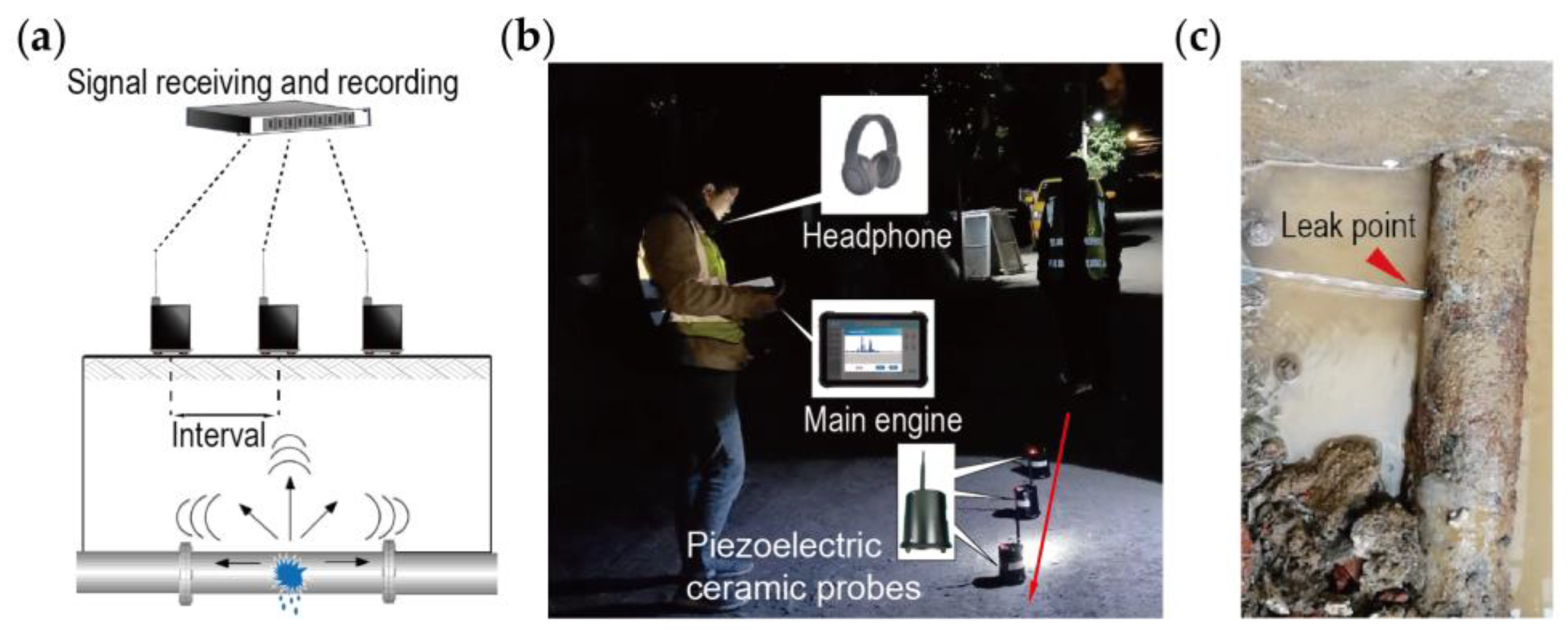
• The present study proposes an effective method for leak detection using ground acoustic signals collected by listening devices, as opposed to methods that use signals from the pipeline wall. This method is based on the fusion of handcrafted features and deep representations, providing a novel approach to leak detection using ground acoustic signals.
• This work innovatively proposes a fusion method that combines handcrafted features with deep representations using a PCNN structure. The effectiveness of this fusion method is demonstrated. The PCNN, integrating handcrafted features and deep representations, outperforms traditional classifiers that rely solely on CNN or handcrafted features. Furthermore, the study extends the application of PCNN and improves the structure of PCNN for leak detection tasks, which is a novel application of PCNN.
• The researchers evaluate the applicability of MFCCs’ features to leak detection in WDS. By combining MFCCs’ features with TFD features, the representation ability of handcrafted features is further investigated.
• Additionally, the work provides insights into the operation and decision-making process of deep learning for leak detection tasks, contributing to the wider understanding of the application of deep learning to pipeline leak signal recognition.

2. Methods

2.1. Convolutional Neural Network

A convolutional neural network (CNN) is a type of deep feedforward neural network that processes data in a mesh structure [39]. In general, a CNN model consists of an input layer, several convolutional and pooling layers, a flatten layer, fully connected layers, and a classification layer (for example, a softmax layer). Utilizing trainable kernel filters, the convolutional layers perform the task of detecting local features in the input feature map. A pooling layer is always located behind a convolutional layer. The dimensionality of the feature map and the number of trainable parameters can be reduced using pooling to achieve sparse processing, and the main representative features of the feature map are determined [40,41]. The extracted feature map is expanded into a one-dimensional vector using the flatten layer, and this allows local features to be integrated globally. The 1D vector is then passed through fully connected layers and a classification layer to obtain the output.

Equation (1) presents the feedforward process of a CNN [40]:

$$f\left(X\right)=f_N\left(\left(\cdot \cdot \cdot f_3\left(f_2\left(f_1\left(X, {\theta }^{\left(1\right)}\right), {\theta }^{\left(2\right)}\right), {\theta }^{\left(3\right)}\right),\cdot \cdot \cdot \right), {\theta }^{\left(N\right)}\right)$$

(1)

where ${\theta }^{\left(1\right)}, {\theta }^{\left(2\right)},\cdot \cdot \cdot , {\theta }^{\left(N\right)}$, including weights and biases, are the training parameters of the $N$ layers; $f_1, f_2,\cdot \cdot \cdot , f_N$ are the operations at each layer; $f\left(X\right)$ is the final output, and $X$ is the input data. In general, the input data for the leak detection task are one-dimensional pressure or acoustic signals.

2.2. The Selected Handcrafted Features

The quality of handcrafted features has a significant impact on the performance of the PCNN model. It is essential to choose features that are robust and generalizable for the leak detection domain. In this paper, the MFCCs’ features and TFD features will be utilized to construct the handcrafted features that will serve as inputs to the PCNN model.

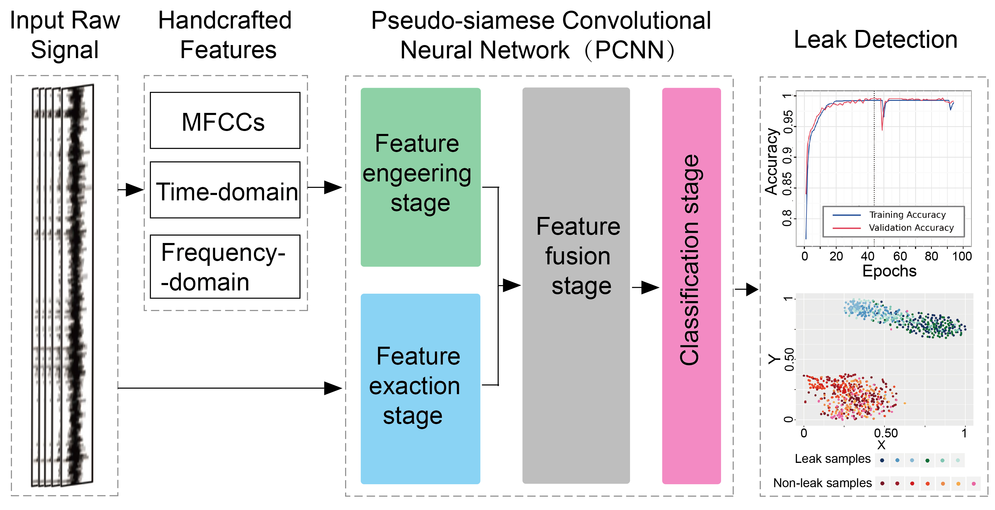
2.2.1. MFCCs’ Features

Human ears respond differently to different frequencies of sound waves. The Mel frequency is more similar to human auditory responses. For this reason, MFCCs’ features show improved robustness compared to traditional auditory features [42]. While MFCCs have received less attention than other handcrafted features in the leak detection field, there are some cases where they have proven effective [43,44,45].

Mel frequency describes the nonlinear characteristic of the human ear. Equation (2) represents the relationship between the Mel frequency and the actual frequency [44]:

$$Mel\left(f\right)=2595log\left(1+\frac{f}{700}\right)$$

(2)

where $f$ is the actual frequency in Hz and $Mel\left(f\right)$ is the Mel frequency. A typical extraction process for MFCCs’ features includes the following steps [46].

The first step involves the preprocessing of the raw signal. As part of the signal preprocessing, pre-emphasizing, framing, and windowing are applied in the respective order. In the next step, the discrete Fourier transform (DFT) of each frame of the signal is performed to obtain its magnitude spectrum.

Then, the Mel spectrum is computed by multiplying the magnitude spectrum by each Mel filter. Mel filters comprise triangular band-pass filters that are based on auditory perception. Figure 1 presents Mel filters and the average MFCCs’ features’ responses. To accomplish the leak detection task in this paper, 24 Mel filters have been designed, with frequencies ranging from 20 Hz to 2000 Hz (see Figure 1a).

In the third step, the discrete cosine transform (DCT) was performed to calculate the MFCCs. In this paper, 13 cepstral coefficients (13th coefficient is energy) were used as the original MFCCs’ features. MFCCs reflect primarily the static characteristics of the acoustic signal. However, the human ear is more sensitive to the dynamic characteristics of acoustic signals [47]. The first- and second-order derivatives of MFCCs’ features can be utilized to describe the dynamic characteristics.

For leak and non-leak signals, Figure 1b shows the average value of the original MFCCs, while Figure 1c,d present that of first- and second-order derivatives of MFCCs, respectively. It is evident that the leak signals and non-leak signals exhibit different static characteristics and dynamic characteristics. In this paper, the MFCCs’ features, comprising 39 coefficients, consist of the original MFCCs’ features and its first-order and second-order derivatives. The MFCCs’ features can be expressed as $\left\{X_{Mel1}, X_{Mel2}, X_{Mel3}\dots , X_{Mel38}, X_{Mel39}\right\}$.

2.2.2. TFD Features

It has been demonstrated that TFD features are very useful for studying leakage mechanisms, and they may directly relate to leakage conditions [10].

Figure 2a,b present time waveforms and frequency spectra of signals for an actual leaking plastic pipe before and after repair. It can be observed that the difference between leak and non-leak signals is evident in both the time domain and frequency domain. In most cases, leak signals contain more energy and have a different frequency range than non-leak signals [48]. The differences between leak and non-leak signals can be well represented by TFD features for identifying leaks.

Table 1. The selected frequency-domain features.

No.	Features	Definition	No.	Features	Definition
1	Peak frequency	$X_{Pf}=f_k,k=\underset{n}{argmax}{s}_n$	4	Root mean square frequency	$X_{Rmf}=\sqrt{X_{Msf}}$
2	Frequency center	$X_{Fc}=\frac{{\displaystyle \sum _{n=1}^N\left(f_n\times s_n\right)}}{{\displaystyle \sum _{n=1}^N{s}_n}}$	5	Frequency variance	$X_{Fv}=\frac{{\displaystyle \sum _{n=1}^N\left[\left(f_n-X_{Fc}\right)\times s_n\right]}}{{\displaystyle \sum _{n=1}^N{s}_n}}$
3	Mean square frequency	$X_{Msf}=\frac{{\displaystyle \sum _{n=1}^N\left(f_n^2\times s_n\right)}}{{\displaystyle \sum _{n=1}^N{s}_n}}$	6	Frequency standard deviation	$X_{Fsd}=\sqrt{X_{Fv}}$

and

Table 2. The selected time-domain features.

No.	Features	Definition	No.	Features	Definition
1	Mean value	$X_M=\frac{1}{N}{\displaystyle \sum _{n=1}^N{x}_n}$	9	Shape factor	$X_{sf}=\frac{X_{Rms}}{X_{ma}}$
2	Mean absolute value	$X_{Ma}=\frac{1}{N}{\displaystyle \sum _{n=1}^N\left|x_n\right|}$	10	Crest factor	$X_{Cf}=\frac{X_{Mas}}{X_{Rms}}$
3	Root mean square	$X_{Rms}={\left[\frac{1}{N}{\displaystyle \sum _{n=1}^N{x}_n^2}\right]}^{1/2}$	11	Impulse factor	$X_{If}=\frac{X_{Mas}}{X_{Ma}}$
4	Maximum absolute value	$X_{Mas}=\max \left|x_n\right|$	12	Clearance factor	$X_{Clf}=\frac{X_{Mas}}{\left(\frac{1}{N}{\displaystyle \sum _{n=1}^N\sqrt{\left|x_n\right|}}\right)}$
5	Standard deviation	$X_{Sd}={\left[\frac{1}{N-1}{\displaystyle \sum _{n=1}^N\left(x_n-X_{Ma}\right)}\right]}^{1/2}$	13	Skewness factor	$X_{Skf}=\frac{X_{Sk}}{X_{Rms}^3}$
6	Peak-peak value	$X_{Ppv}=\max \left(x_n\right)-\min \left(x_n\right)$	14	Kurtosis factor	$X_{Kuf}=\frac{X_{Ku}}{X_{Rms}^4}$
7	Skewness	$X_{Sk}=\frac{{\displaystyle \sum _{n=1}^N{\left(x_n-X_{Ma}\right)}^3}}{\left(N-1\right)X_{Sd}^3}$	15	Margin factor	$X_{Mf}=\frac{X_{Ma}}{{\left(\frac{1}{N}{\displaystyle \sum _{n=1}^N\sqrt{\left|x_n\right|}}\right)}^2}$
8	Kurtosis	$X_{Sk}=\frac{{\displaystyle \sum _{n=1}^N{\left(x_n-X_{Ma}\right)}^3}}{\left(N-1\right)X_{Sd}^3}$

describe the selected frequency- and time-domain features, respectively. These features are the most common TFD features [10,49]. In Table 1, $s_m$ and $f_m$ are the spectral amplitude and the corresponding frequency scale for $m=1, 2, \dots , M$, and $M$ is their length in frequency scale. In Table 2, $x_n$ represents a time series for $n=1, 2, \dots , N$, and $N$ is the length of the samples. In the present paper, these TFD features can be expressed as $\left\{X_M, X_{Ma}, X_{Rms}\dots , X_{Fv}, X_{Fsd}\right\}$.

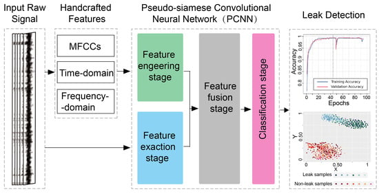
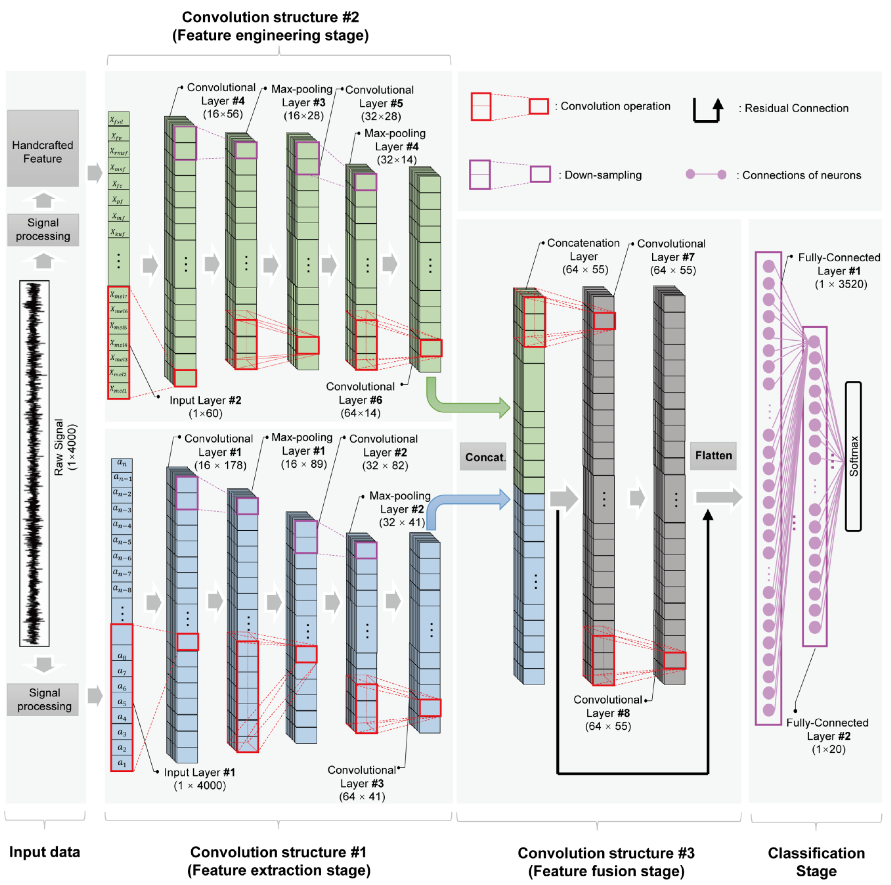
2.3. Pseudo-Siamese Convolutional Neural Network for Feature Fusion

For feature fusion, it is not recommended to contact handcrafted features and raw signals directly in the input layer due to their different scale and spatial relationship. The flexible design of the PCNN structure allows inputs with different scales and spatial relationships to be processed through two parallel convolutional streams that do not share weights. This is why PCNN was chosen for feature fusion.

Figure 3 shows the architecture of PCNN used in this paper, and the hyperparameters of the network have been optimized. The PCNN employs two independent convolutional structures to process the input handcrafted features and raw signals in parallel.

At a higher level, another convolutional structure is used to fuse the obtained information. In the PCNN model, there are four stages with different functions: the feature extraction stage, the feature engineering stage, the feature fusion stage, and the classification stage.

2.3.1. Feature Engineering Stage

As shown in Figure 3, the feature engineering stage is composed of an input layer, three convolutional layers, and two pooling layers. The input layer of the feature engineering stage is populated with 60 handcrafted features that are derived from the original signals. The convolutional and pooling layers enable CNNs to effectively reduce dimensionality and extract features. It is expected that the model give less attention to handcrafted features with low leak discriminatory power after being processed. This will be further illustrated in Section 3.5.

The convolutional layers receive features from the input layer. The convolutional layers perform the task of feature engineering with trainable kernel filters. The convolutional stride is set to 1 due to the small scale of the input. Two max-pooling layers (stride = 2) follow the corresponding convolutional layers to downsample the feature maps.

The activation function used throughout this paper is ReLU because it is more efficient and solves the vanishing gradient problem. The feature engineering stage is designed such that the main representative features of the input handcrafted features are determined.

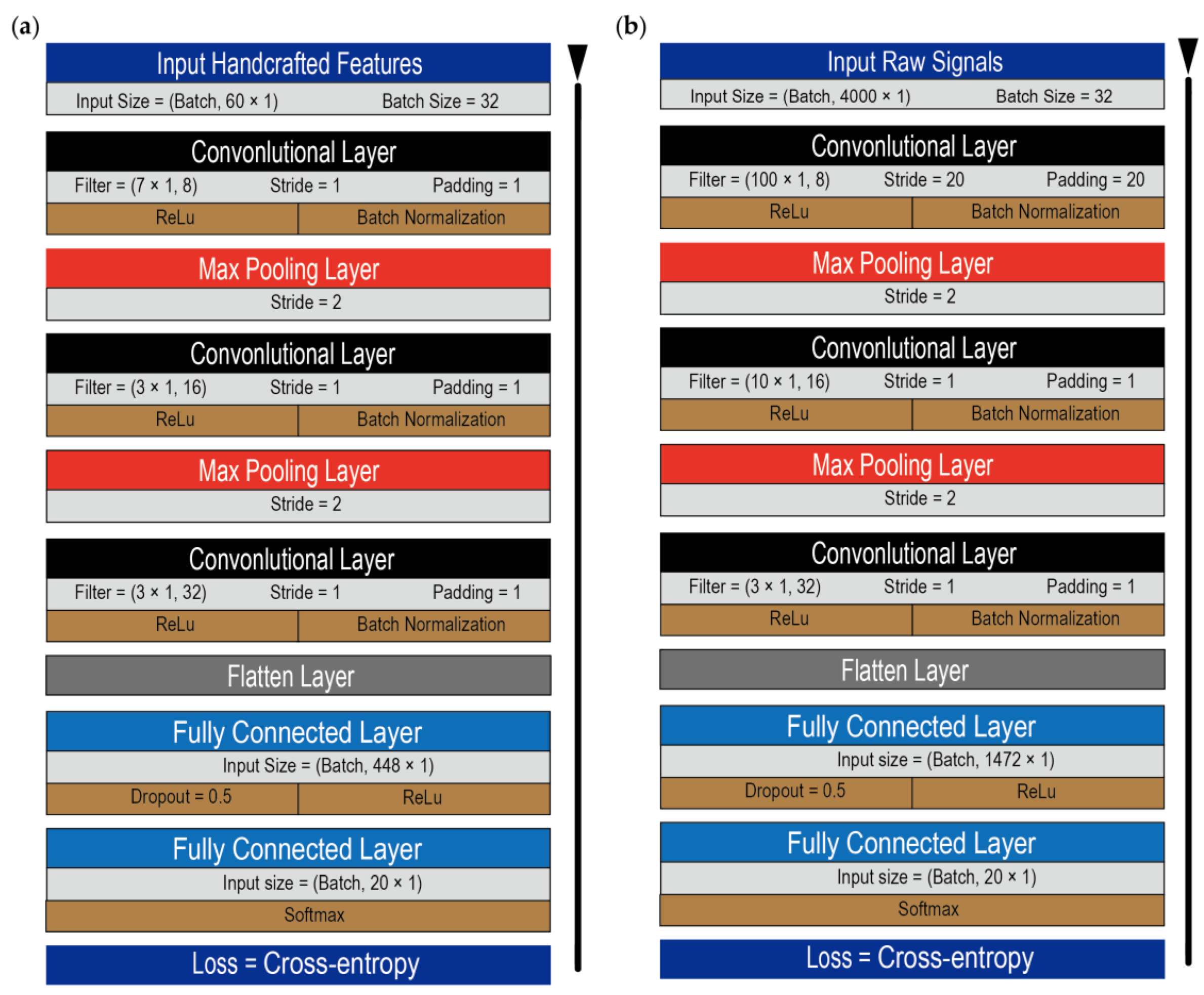
2.3.2. Feature Extraction Stage

The feature extraction stage utilizes a similar network architecture as the feature engineering stage, but with different hyperparameters. Multiple convolutional layers and pooling layers are used in the feature extraction stage. The local features and macro features in the one-dimensional time series are automatically extracted and expressed in the output feature maps.

Relatively large filters are used in the first and second convolutional layers of the feature extraction stage. The fact is that a large filter will have a larger receptive field [50], which will allow more macro features to be extracted. Additionally, a larger stride is selected for the convolutional layer to reduce the feature map dimensionality more rapidly. The idea is that the output feature maps of the feature extraction and feature engineering stages will reach the same scale to facilitate feature fusion.

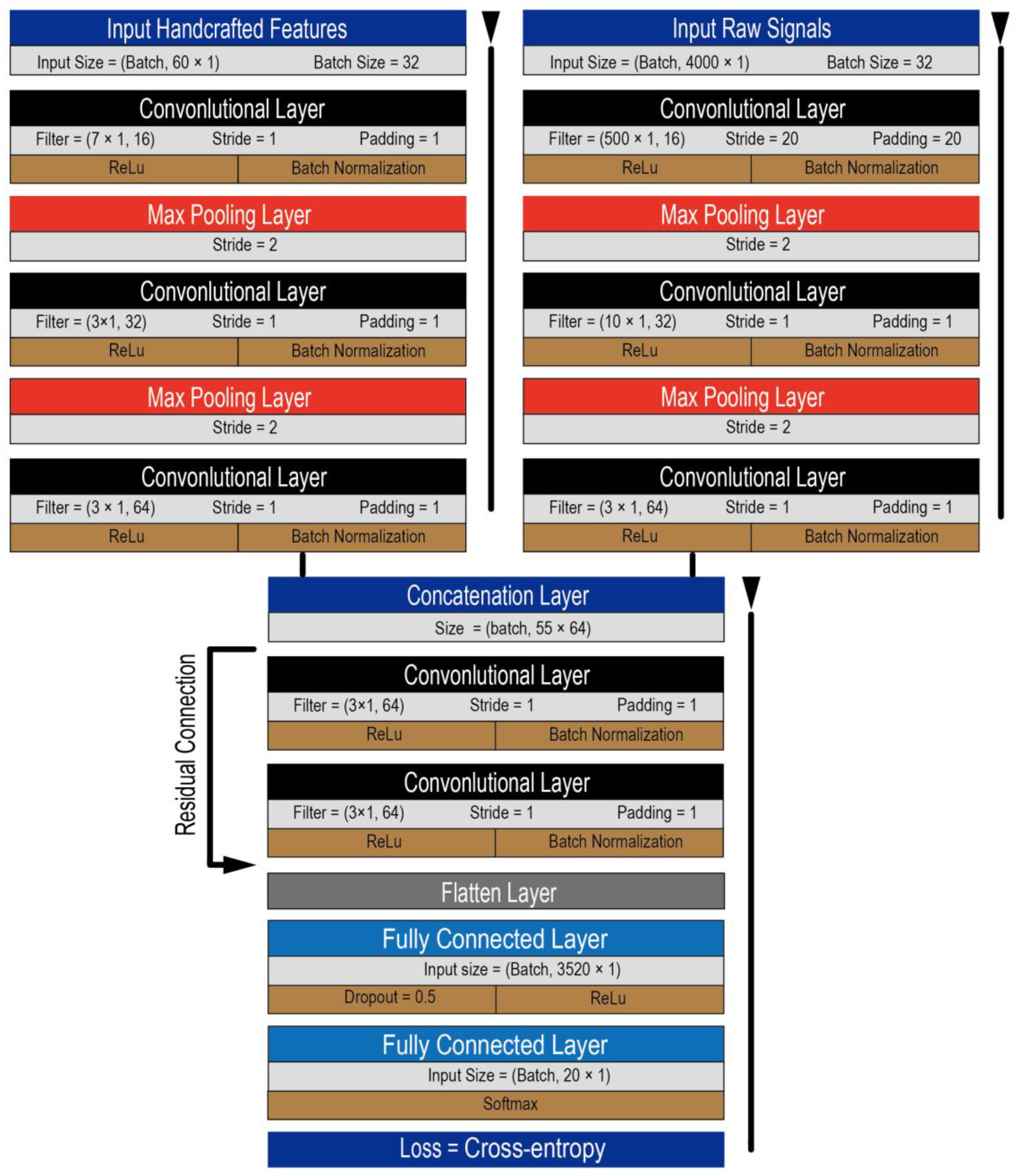
2.3.3. Feature Fusion Stage and Classification Stage

Figure 3 shows the feature fusion stage comprises a concatenation layer and two convolutional layers. The output feature maps of the first two convolutional streams are concatenated in the concatenation layer. The feature maps of the concatenation layer are then passed through the convolutional layers in order to learn fusion rules and create new features that are more integrated. In the feature fusion stage, the 3 × 1 filters, with stride and padding of 1, are used in the convolutional layers to maintain the spatial resolution of feature maps. However, the max-pooling layer is also omitted. A residual connection is used to build an identity map between the concatenation layer and the output of the feature-fusion stage. A deep CNN is susceptible to losing feature information in the forward training process [34]. The problem can be eliminated by utilizing residual connections.

2.3.4. Classification Stage and Loss Function

The classification stage consists of two fully connected layers and a classification function. The output feature map of the feature fusion stage is flattened and used as an input for the first fully connected layer. The output of the second fully connected layer is connected to a softmax function to obtain the final output of the PCNN model.

The loss function measures the difference between the target output and the CNN prediction. In the process of minimizing the loss function, all learnable weights and biases are updated. Binary cross-entropy loss is used to train our model, and this function is expressed in Equation (3), as follows:

$$Loss=-\frac{1}{N}{\displaystyle \sum _n{\displaystyle \sum _{i=1}^M\left(Y_{ni}log{y}_{ni}\right)}}$$

(3)

where $Y_{ni}$ and $y_{ni}$ are the actual label and the predicted output value of the sample, respectively, $i$ is the number of classes in the $n$th sample, $N$ is the total number of samples, and $M$ is the number of classes.

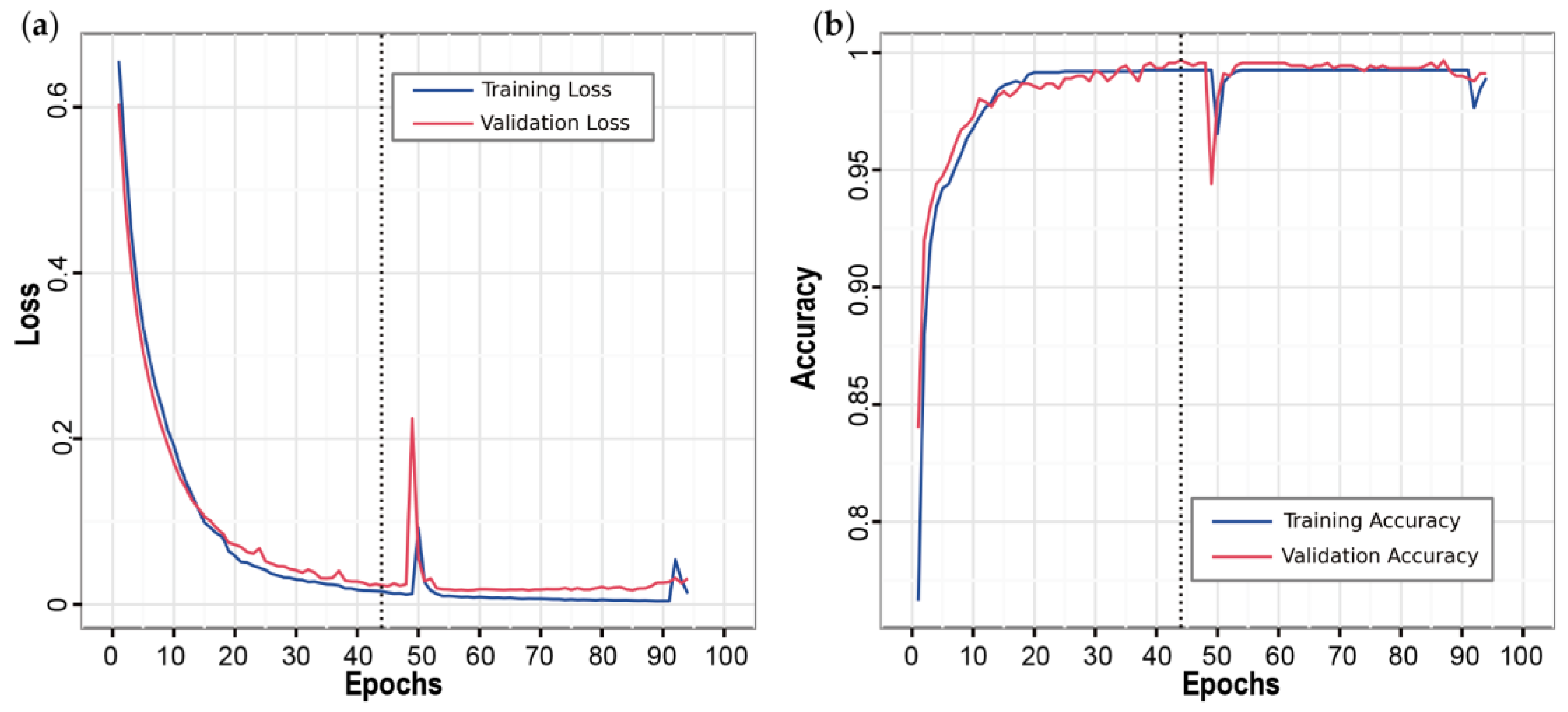
2.3.5. Network Training

All convolutional layers are initialized using the Kaiming initialization method [51]. The loss function is optimized using a Nesterov-accelerated adaptive moment estimation (Nadam) [52] optimizer (${\beta }_1=$ 0.9, ${\beta }_2=$ 0.999) with a momentum decay $\psi =$ 0.004, a weight decay $\lambda =$ 0.01, a learning rate $lr=$ 0.0001, a batch size of 32, and early stopping with a patience of 50 epochs. The optimal learning rate and batch size for the model were determined by testing all possible combinations of $lr\in$ {0.005, 0.001, 0.0005, 0.0001, 0.00005, 0.00001} and batch size $\in$ {8, 16, 32, 64}.

It is shown that Nadam is computationally efficient and converges faster than standard stochastic gradient methods [53]. To speed up the training and prevent overfitting, the fully connected layer employs dropout with a parameter of 0.5, while the convolutional layer employs batch normalization.

2.4. Experiments Settings

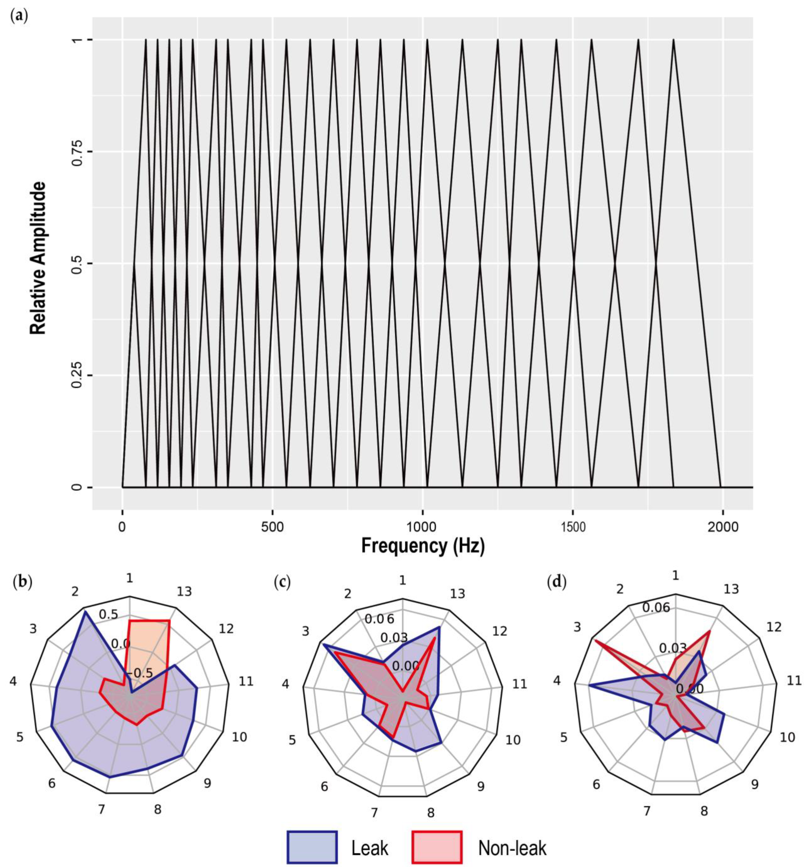
2.4.1. Case Study and Data Set

Several leak and non-leak signals from actual pipe leaks as well as some environmental noise were collected for the purpose of developing an intelligent algorithm (the PCNN model, which combines handcrafted features and deep representations).

Figure 4 shows the in situ signals’ acquisition on the ground in WDS. The data were collected during the leak detection project of the Hunan Puqi Water Environment Institute in Changsha City from 2017 to 2022.

Figure 4b shows a site photo of the leak signal collection, while Figure 4c shows the leak point after excavation. In the detected pipelines, the diameters range from DN50 to DN300 mm, buried depths range from 0.6 to 2.4 m, and the pressure ranges from 0.2 to 0.4 MPa. The detected pipes are plastic or metal. The plastic pipes are mainly polyvinyl chloride (PVC) or polyethylene (PE) pipes, while steel pipes or cast iron pipes comprise the majority of the metal pipes.

In the project, leaks were located using a combination of several techniques such as leak noise correlators, listening rods, and electronic amplified listening devices. Once the leaks were located, the electronic amplified listening devices (PQWT-LDC) measured and stored the vibration. The PQWT-LDC comprises piezoelectric ceramic probes, headphones, and a basic engine with wireless communication (see Figure 4b).

In Figure 4a, piezoelectric ceramic probes are placed on the ground surface along the pipeline at a certain interval to collect vibrations. Then, the signals are transmitted to the main engine through wireless communication and stored there. To ensure the quality of signal acquisition, the electronic amplified listening devices are calibrated before each collection. The sample rate is set to 8000 Hz. According to the Nyquist–Shannon sampling theorem, the sample rate is adequate to capture the effective bandwidth [48] (generally below 3000 Hz) of leak signals for both plastic and metal pipes.

A total of 142 leak cases were obtained in this leak detection project, after excluding misjudged leaks. For each leak case, the selected leak signal was the vibration collected by the closest probe to the actual leak position. Because the interval is set to 1.0 m, the leak signal was collected within a horizontal distance of 1.0 m from the actual leak position. After each leaking pipe was repaired, the normal-state signals of the repaired pipes were collected under the same conditions that the leak signals were collected.

Table 3. The signals collected in the actual WDS.

State	Categories	Materials	Burial Depth (m)	Case Number
Leak	L1	Plastic	0.6~1.2	40
	L2	Plastic	1.2~1.8	27
	L3	Plastic	1.8~2.4	17
	L4	Metal	0.6~1.2	28
	L5	Metal	1.2~1.8	21
	L6	Metal	1.8~2.4	9
Non-leak	N1	Plastic	0.6~1.2	40
	N2	Plastic	1.2~1.8	27
	N3	Plastic	1.8~2.4	17
	N4	Metal	0.6~1.2	28
	N5	Metal	1.2~1.8	21
	N6	Metal	1.8~2.4	9
	N7 (Noise)	/	/	20

shows the collected signals in the study. The collected signals are represented by two states: leak (L) and non-leak (N). Additionally, typical noises such as traffic noise and construction noise are collected and classified as environmental noise group N₇.

Each signal is collected for 5 s, and its length is 40,000 points. For machine learning purposes, the obtained signals are divided into samples with a length of 4000 points, resulting in 1420 leak signals and 1620 non-leak signals in the dataset. The dataset is preprocessed using linear detrending and normalization. In this study, 70% of the dataset is used for training and 30% for testing. To obtain a reliable model, the 10-fold cross validation method [54] is employed. To accomplish the machine learning task, the applications utilized include 64-bit Windows 10, PyTorch, and an NVIDIA GeForce GTX1050 Ti, together with Python3. Signal preprocessing and handcrafted feature computing are both performed in Python3.

2.4.2. Evaluation Metrics

The performance of different leak detection architectures and methods are evaluated with a confusion matrix and four metrics: accuracy (Acc), sensitivity (Sen), specificity (Spe), and $F_1\text{-}score$. Equations (4)–(7) give the four metrics.

$$Acc=\frac{\left(TP+TN\right)}{(TP+TN+FP+FN)}$$

(4)

$$Sen=\frac{\left(TP\right)}{(TP+FN)}$$

(5)

$$Spe=\frac{\left(TN\right)}{(TN+FP)}$$

(6)

$$F_1\text{-}score=\frac{2}{(2+\frac{FP}{TP}+\frac{FN}{TP})}$$

(7)

where TP, TN, FP, and FN denote the number of the true positive samples, the true negative samples, the false positive samples, and the false negative samples, respectively. In this paper, positive samples refer to leak samples. Additionally, the confusion matrix offers a clear visualization of TP, TN, FP, and FN, making it an important tool for evaluating the model’s performance.

2.5. Model Visualization and Interpretation Method

Analysis or visualization of internal structures or processes is particularly useful for elucidating how the deep learning model operates [55]. After constructing, training and testing the PCNN, an interpretable understanding of the model is obtained to support its effectiveness. To visualize the feature map distribution of different samples in the model feedforward process, the t-distributed stochastic neighbor embedding [56] (t-SNE) method is used. The saliency map [57] is used to analyze the influence of the input on decision-making.

2.5.1. T-SNE for Model Visualization

Analyzing the representation of different category samples in the model can be helpful in gaining a better understanding of the model. There are high-dimensional data present in the input to the PCNN and the feature maps of different layers of the PCNN. In the field of modern machine learning, visualizing high-dimensional data can be considered one of the most fundamental tasks. In terms of high-dimensional data visualization with intrinsic clusters, the t-distributed stochastic neighbor embedding (t-SNE) algorithm was widely recognized in the literature as an advanced technique [58,59]. The idea behind t-SNE is to minimize the Kullback–Leibler divergence between the distribution of pairwise similarities in the input space and their embedded samples in low dimensions. For this reason, t-SNE, as a non-linear dimensionality reduction technique, is able to solve the crowding problem while preserving more local features of the original data, when compared with traditional methods such as principal component analysis (PCA).

2.5.2. Saliency Map Based on Vanilla Gradient

The saliency map is the heat map that visualizes the relevance between the feature or data point in the input example and the prediction of the model. The Vanilla gradient algorithm [57] is the original saliency map algorithm for supervised deep learning. Quantitative evaluation of the Vanilla gradient has demonstrated that it is relatively robust in comparison with other algorithms. In addition, this algorithm is the simplest of all gradient-based methods and runs very quickly. The Vanilla gradient is implemented by calculating the gradient of the loss function for the class that is being analyzed in relation to the input pixels.

In this paper, the Vanilla gradient is used to analyze the relevance of input. The saliency maps will highlight features or regions that are more critical to individual predictions.

Equation (8) gives an expression for the relevance score obtained by computing the gradient of each class score functions with respect to the input sample [57]:

$$R\left(I_0\right)=\frac{\partial S_C\left(I\right)}{\partial I}{|}_{I=I_0}$$

(8)

Here, $S_C\left(I\right)$ is the score function of input $I$ for class c. $R\left(I_0\right)$ is the relevance score, calculated as the derivative of $S_C\left(I\right)$ with respect to $I=I_0$. The symbol $I_0$ denotes an input sample. Then, the relevance score can be visualized for each feature to highlight contributions to decision-making. The absolute value of gradient maps is chosen in this paper because it is clear in visualization.

3. Results and Discussion

3.1. Architectures and Hyperparameters Optimization

Previous studies [60,61] showed that the number of convolutional layers and the size and the number of filters influence the effectiveness of CNN. To improve the performance of the PCNN model, the appropriate hyperparameters and structures must be determined.

First, the effect of hyperparameters on the feature extraction and feature engineering stage is investigated. This is based on the reference CNN architectures in presented in Figure 5a and Figure 5b, respectively. Then, the effect of hyperparameters on the feature fusion stage is investigated, using a new reference model presented in Figure 6, after the hyperparameters of the two previous stages have been determined. The performance of variants of the reference models is presented in

Table 4. The performance of convolutional neural networks with handcrafted features as input. These convolutional neural networks are variants of the reference model presented in Figure 5a.

No.	Layers	Kernel Size	Filters Number	Evaluation Criteria (%)				Para. Count
				Acc	Sen	Spe	F1-Score
1	3	7-3-3	8-16-32	98.88 ± 0.46	98.85 ± 0.52	98.91 ± 0.64	98.88 ± 0.47	11,166
2	3	5-3-3	8-16-32	98.68 ± 0.29	99.23 ± 0.36	98.21 ± 0.57	98.65 ± 0.30	11,150
3	3	9-3-3	8-16-32	98.62 ± 0.35	99.13 ± 0.30	98.17 ± 0.59	98.58 ± 0.36	10,542
4	3	11-3-3	8-16-32	98.51 ± 0.65	98.97 ± 0.32	98.11 ± 1.12	98.47 ± 0.68	10,558
5	3	15-3-3	8-16-32	98.11 ± 0.85	98.62 ± 0.87	97.67 ± 1.11	98.07 ± 0.87	9950
6	3	7-3-3	16-32-64	99.35 ± 0.17	99.62 ± 0.24	99.12 ± 0.34	99.33 ± 0.17	26,110
7	3	7-3-3	32-64-128	99.24 ± 0.20	99.53 ± 0.26	98.99 ± 0.36	99.22± 0.21	67,518
8	2	7-3	16-32	97.98 ± 0.84	97.96 ± 0.99	98.00 ± 0.99	97.97 ± 0.85	19,774
9	5	7-3-3-3-3	16-32-64-64-64	99.19 ± 0.26	99.51 ± 0.34	98.91 ± 0.45	99.16 ± 0.29	51,070
10	5 *	7-3-3-3-3	16-32-64-64-64	99.34 ± 0.29	99.88 ± 0.12	98.87 ± 0.55	99.31 ± 0.31	51,070
11	7	7-3-3-3-3-3-3	16-32-64-64-64-64-64	98.98 ± 0.60	99.37 ± 0.55	98.64 ± 0.80	98.95 ± 0.62	76,030
12	7 *	7-3-3-3-3-3-3	16-32-64-64-64-64-64	99.16 ± 0.36	99.55 ± 0.19	98.81 ± 0.66	99.13 ± 0.38	76,030

Note(s): * in the upper right corner of the layer number indicates that the network has applied residual connections.

,

Table 5. The performance of convolutional neural networks with raw signals as input. These convolutional neural networks are the variants of the reference model presented in Figure 5b.

No.	Layers	Kernel Size	Filters Number	Evaluation Criteria (%)				Para. Count
				Acc	Sen	Spe	F1-Score
1	3	50-10-3	16-32-64	95.88 ± 1.36	95.87 ± 2.02	95.88 ± 1.60	95.86 ± 1.36	71,342
2	3	30-10-3	16-32-64	94.67 ± 1.74	94.20 ± 2.97	95.08 ± 2.04	94.68 ± 1.71	71,022
3	3	100-10-3	16-32-64	96.28 ± 1.02	96.29 ± 1.04	96.28 ± 1.40	96.26 ± 1.03	72,142
4	3	200-10-3	16-32-64	97.84 ± 0.82	97.28 ± 0.95	98.33 ± 1.18	97.86 ± 0.84	71,182
5	3	500-10-3	16-32-64	98.42 ± 0.56	98.71 ± 0.59	98.17 ± 0.79	98.39 ± 0.58	72,142
6	3	1000-10-3	16-32-64	98.19 ± 0.60	98.64 ± 0.81	97.80 ± 0.80	98.15 ± 0.61	71,182
7	3	500-3-3	16-32-64	98.15 ± 0.67	98.73 ± 0.85	97.63 ± 0.65	98.10 ± 0.66	72,398
8	3	500-5-3	16-32-64	98.27 ± 0.34	97.93 ± 0.65	98.56 ± 0.64	98.28 ± 0.35	72,142
9	3	500-20-3	16-32-64	98.22 ± 0.80	98.47 ± 0.41	98.00 ± 1.46	98.20 ± 0.83	70,862
10	3	500-10-3	32-64-128	98.43 ± 0.41	98.57 ± 0.88	98.31 ± 0.52	98.41 ± 0.40	166,750
11	3	500-10-3	8-16-32	97.17 ± 0.84	97.02 ± 1.54	97.30 ± 0.96	97.16 ± 0.83	33,286
12	2	500-10	16-32	97.41 ± 0.98	96.78 ± 1.92	97.96 ± 1.21	97.44 ± 0.96	65,806
13	5	500-10-3-3-3	16-32-64-64-64	98.26 ± 0.39	99.06 ± 0.47	97.55 ± 0.78	98.20 ± 0.41	97,102
14	5 *	500-10-3-3-3	16-32-64-64-64	98.45 ± 0.61	98.80 ± 0.66	98.15 ± 0.76	98.42 ± 0.61	97,102
15	7	500-10-3-3-3-3-3	16-32-64-64-64-64-64	98.11 ± 0.62	98.90 ± 0.42	97.43 ± 1.09	98.06 ± 0.64	122,062
16	7*	500-10-3-3-3-3-3	16-32-64-64-64-64-64	98.23 ± 0.54	98.57 ± 0.41	97.94 ± 1.02	98.21 ± 0.57	122,062

Note(s): * indicates the residual connections.

, and

Table 6. The performance of pseudo-siamese convolutional neural networks based on the structure in Figure 6.

No.	Layers	Residual Connection	Evaluation Criteria (%)				Para. Count
			Acc	Sen	Spe	F1-Score
1	2	Yes	99.70 ± 0.12	99.93 ± 0.15	99.51 ± 0.21	99.69 ± 0.13	123,150
2	2	No	99.50 ± 0.17	99.72 ± 0.18	99.30 ± 0.25	99.48 ± 0.18	123,150
3	4	Yes	99.46 ± 0.20	99.44 ± 0.22	99.49 ± 0.31	99.46 ± 0.21	148,110
4	4	No	99.27 ± 0.27	99.62 ± 0.11	98.95 ± 0.47	99.24 ± 0.28	148,110
5	6	Yes	99.44 ± 0.22	99.74 ± 0.16	99.18 ± 0.40	99.42 ± 0.23	173,070

, respectively.

The structure and hyperparameters have a significant impact on the performance of the reference models. From Table 4, the model number 6 has the highest accuracy and F₁-score, compared with the models number 10 and 7.

Figure 7 and Figure 8 present the average confusion matrices of the 12 models in Table 4. The findings suggest that model 6 exhibits superior performance in identifying negative samples, whereas model 10 excels at recognizing positive samples but performs relatively worse in identifying negative samples compared to model 6. Additionally, model 6 features a simpler structure which facilitates subsequent feature fusion. Based on the results, the hyperparameters and architecture of model 6 were chosen for the feature engineering stage.

By contrast, Table 5 shows the performance of model 5 is slightly lower than that of models 10 and 14.

Figure 9 and Figure 10 show the average confusion matrices of the 16 models in Table 5. The results indicate that model 8 exhibits the best performance in identifying negative samples, while model 13 shows the best performance in recognizing positive samples, although neither of them demonstrate remarkable performance on the overall dataset. Additionally, it can be observed that as the complexity of the model increases, the CNN with raw signals as input enhances its ability to identify positive samples, but diminishes its ability to identify negative samples. Models 5, 10, and 14 show good performance on the overall dataset. However, model 5 has fewer parameters, and a smaller convolution depth that reduces the risk of overfitting. Based on these results, the hyperparameters and architecture of model 5 were selected for the feature extraction stage.

For a single stage, a convolutional structure with 2-3 convolutional layers can extract features from the input signal effectively. Other scholars drew a similar conclusion in their studies on leak identification [18,49]. Performance degradation may occur as the network gets larger. This is usually caused by vanishing gradients or exploding gradients as the network depth increases, rather than overfitting. The vanishing gradient problem can cause higher test and training errors.

Furthermore, experimental results indicate that the number of convolution kernels does not always have a positive effect. It is also possible for models with too many layers of convolution and too many convolution kernels to become overfitted, thereby reducing their computational efficiency.

Moreover, the use of large kernels is particularly advantageous for CNNs with raw acoustic signals as input. As shown in Table 5, the network performed better when the kernel size of the first convolutional layer was set to 500. Further, changing the kernel size of the first convolutional layer to 1000 without changing the filter number can cause drops in performance due to only macroscopic features being extracted by the network. The reason supporting the use of a large kernel may be the larger effective receptive field. According to Hanin et al. [62], neural networks require sufficient width, whereas simply increasing the depth does not guarantee the network’s generalization capacity. In addition, using a wide kernel in the first convolutional layer of a convolutional neural network can suppress noise [63].

Table 6 shows the optimization results of the PCNN. Based on these results, the model number 1 was selected. By using the residual connection, the network degradation problem associated with a too-deep network can be avoided.

Figure 11 presents the average confusion matrices of the five models listed in Table 6. Model 1 demonstrates a strong identification capability for positive samples. Additionally, it can be observed that residual connections enhance the overall identification performance of the models on the dataset.

As can be seen in Table 6, the performance of the PCNN with four convolutional layers in the feature fusion stage is even lower than that of the network with two convolutional layers when the residual connection is not used. Therefore, it appears that deeper networks are more difficult to optimize.

The model optimization helped determine the optimal hyperparameters and architecture (same as the reference model in Figure 6) of the PCNN.

Figure 12a,b show the loss and accuracy of the optimized PCNN for one trial. The presence of spikes on both the loss function and accuracy curve can be attributed to the fact that the dataset cannot be evenly partitioned by the batch size. As a result, some mini-batches contain insufficient data, which in turn causes abnormal fluctuations during the model training process. The PCNN converges fast, within 50 epochs, and exhibits excellent classification performance. There is an average validation accuracy of 99.70% with a standard deviation of 0.12% for the ten trials.

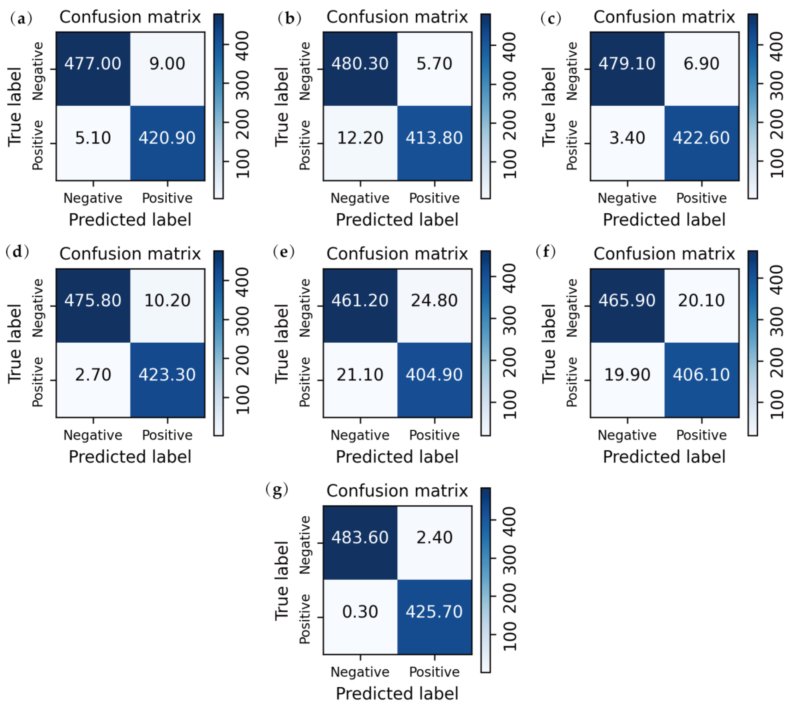
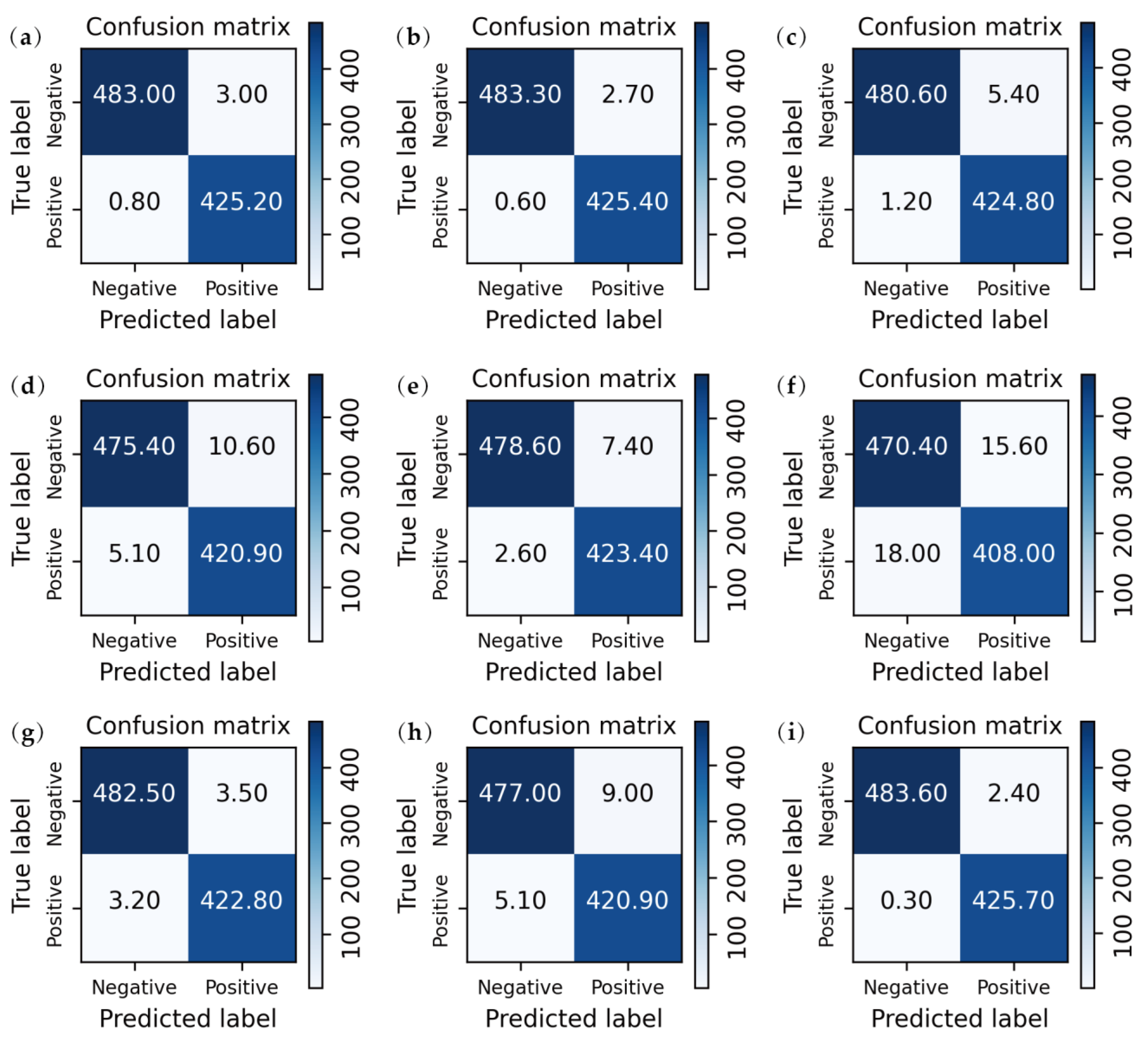
3.2. Performance Comparison

Based on the dataset obtained, the effectiveness of the PCNN is compared with other leak detection frameworks (for water or gas pipes) proposed by other scholars. The results are illustrated in

Table 7. Performance comparison among different leak detection frameworks.

Input	Method	Evaluation Criteria (%)
		Acc	Sen	Spe	F1-Score
Raw signals	CNN [49]	98.45 ± 0.61	98.80 ± 0.66	98.15 ± 0.76	98.42 ± 0.61
Raw signals	EEMD+CNN [64]	98.04 ± 0.56	97.14 ± 1.07	98.83 ± 0.40	98.08 ± 0.53
Raw signals	Ensemble 1D-CNN-SVM [18]	98.87 ± 0.26	99.20 ± 0.35	98.58 ± 0.46	98.84± 0.26
2D MFCCs	CNN [44]	98.59 ± 0.49	99.37 ± 0.26	97.90 ± 0.82	98.54 ± 0.51
TFD features	KPCA-SVM [65]	94.97 ± 1.70	95.05 ± 2.24	94.90 ± 2.31	94.94 ± 1.71
Wavelet features	SVM [66]	95.61 ± 1.44	95.33 ± 1.66	95.86 ± 2.02	95.61 ± 1.47
MFCCs + TFD features + Raw signals	PCNN	99.70 ± 0.12	99.93 ± 0.15	99.51 ± 0.21	99.69 ± 0.13

.

From Table 7, the PCNN with MFCCs’ and TFD features and raw signals as input performed better than other leak detection frameworks with partial features, indicating that feature fusion helps the model achieve better detection performance. However, the CNN and ensemble 1D-CNN-SVM with the original signal as input perform better than the SVM with TFD features or wavelet features, indicating that CNN can extract representative features from raw signals for leak detection. Additionally, CNN with 2D MFCCs as input performed better than the CNN with raw signals, showing that MFCCs’ features are particularly useful for leak detection tasks.

Figure 13 shows the average confusion matrix of the seven models listed in Table 7. It can be observed that except for PSCNN, the CNN with 2D MFCCs as input exhibits the second highest recognition capability for positive samples. In addition, compared to the HFB classifier, the CNN structure appears to have stronger recognition capability for negative samples. Moreover, the PCNN has the best recognition capability for both positive and negative samples.

It can be inferred that the PCNN shows superior performance over other leak detection frameworks due to the use of MFCCs’ features and the architecture of feature fusion.

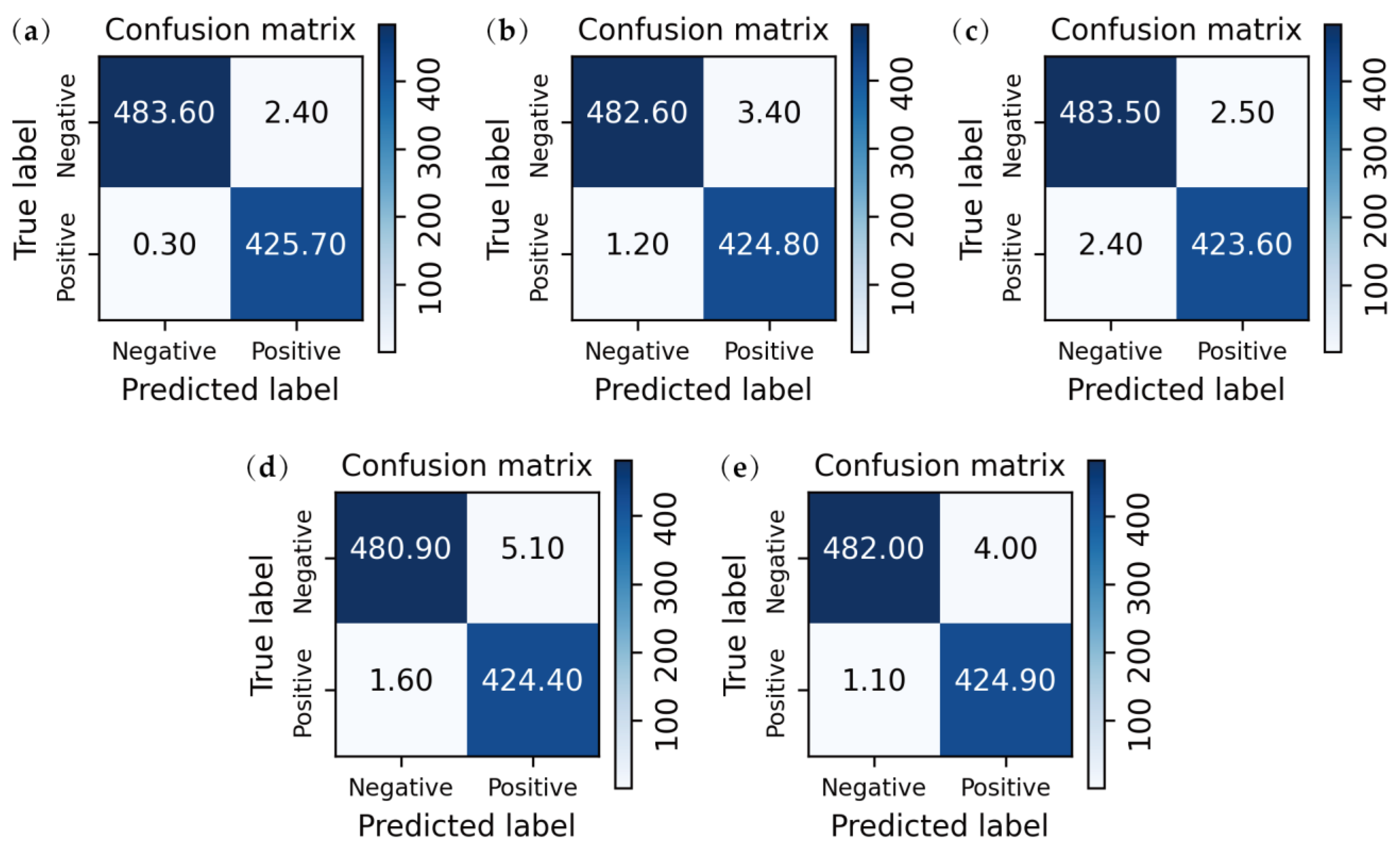
3.3. Quantitative Analysis

In this study, a quantitative analysis of the PCNN model is conducted to study the effect of the input and feature fusion framework. In

Table 8. Quantitative comparison among different methods.

Method	Evaluation Criteria (%)
	Acc	Sen	Spe	F1-Score
PCNN-MLP	99.58 ± 0.19	99.81 ± 0.14	99.38 ± 0.31	99.57 ± 0.20
PCNN-MFCCs&Raw	99.64 ± 0.20	99.86 ± 0.11	99.44 ± 0.29	99.62 ± 0.20
PCNN-TFD&Raw	99.28 ± 0.23	99.72 ± 0.20	98.89 ± 0.33	99.25 ± 0.23
PCNN-Raw&Raw	98.28 ± 0.63	98.80 ± 0.60	97.82 ± 0.53	98.24 ± 0.64
CNN-MFCCs	98.90 ± 0.40	99.39 ± 0.26	98.48 ± 0.67	98.87 ± 0.42
CNN-TFD	94.32 ± 0.76	95.77 ± 1.46	96.79 ± 1.21	96.33 ± 0.76
CNN-MFCCs&TFD	99.27 ± 0.27	99.25 ± 0.40	99.28 ± 0.36	99.26 ± 0.28
CNN-Raw	98.45 ± 0.61	98.80 ± 0.66	98.15 ± 0.76	98.42 ± 0.61
PCNN	99.70 ± 0.12	99.93 ± 0.15	99.51 ± 0.21	99.69 ± 0.13

, a performance comparison is presented between the optimized PCNN, its four variants, and four CNN models that have only one convolutional stream receiving inputs.

In Table 8, PCNN-MLP denotes the PCNN without the feature fusion stage, PCNN-MFCCs&Raw denotes the PCNN with MFCCs’ features and raw signals as input, PCNN-TFD&Raw denotes the PCNN with TFD features and raw signals as input, PCNN-Raw&Raw represents the PCNN wherein both convolutional streams take the raw signal as input, CNN-MFCCs denotes the CNN with MFCCs’ features as input, CNN-TFD denotes the CNN with TFD features as input, CNN-MFCCs&TFD denotes the CNN with the whole handcrafted features as input, and CNN-Raw denotes the CNN with raw signals as input.

The results show that PCNN-MFCCs&Raw, PCNN-TFD&Raw, and PCNN-MLP perform better than CNN-MFCCs, CNN-TFD, CNN-MFCCs&TFD, and CNN-Raw, indicating that feature fusion of handcrafted features and raw signals helps to achieve improved performance.

Figure 14 displays the average confusion matrix of the nine models listed in Table 8. It can be observed that all PCNN models using handcrafted features and raw signals as inputs exhibit excellent recognition capability for positive samples. In terms of recognizing both positive and negative samples, CNN-MFCCs outperforms CNN-Raw, highlighting the powerful capability of MFCCs.

Notably, PCNN-Raw&Raw did not demonstrate superior performance compared to CNN-Raw. It is speculated that this may be due to the fact that both convolutional streams in PCNN utilize raw signals as inputs, which does not fundamentally differ from employing twice the number of convolutional kernels in CNN. The inferior performance of PCNN-Raw&Raw, relative to CNN-Raw, could be attributed to the limited information exchange between the two streams, which primarily occurs at a higher level and may thus contribute to the deterioration of performance to some extent. Accordingly, the result shows that the approach of utilizing multiple identical inputs to construct a PCNN, or even a three-channel convolutional neural network, may be infeasible. Additionally, it can be inferred that the fusion of handcrafted features and deep representation is the crucial factor for improving model performance, rather than the utilization of a PCNN.

In addition, CNN-MFCCs performs better than CNN-TFD and CNN-Raw, which suggests that MFCCs’ features are more effective for leak detection than TFD features or deep representations. CNN-MFCCs&TFD presents a better result than CNN-TFD and CNN-MFCCs, indicating that MFCCs’ and TFD features complement each other. This proposed leak detection framework, which incorporates MFCCs’ features, TFD features, and raw signals as input and performs feature fusion using multiple convolutional streams, demonstrates the highest accuracy.

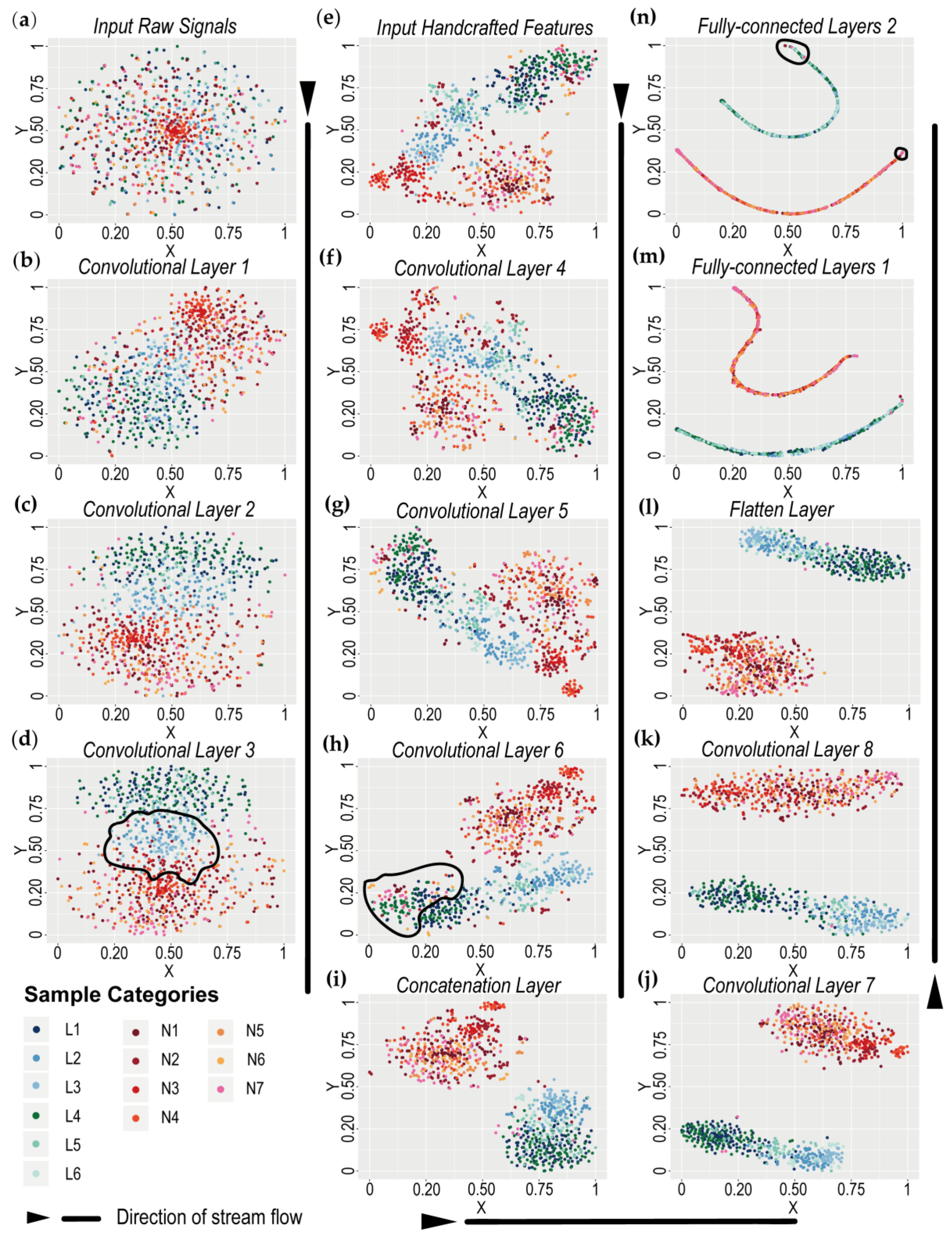
3.4. Model Visualization

The research goal is to study how leak and non-leak signals are distinguished in the feedforward process of a PCNN, and study which stage plays the most critical role.

Figure 15 presents the feature map distributions of the input layers and inner layers of a PCNN visualized with t-SNE.

In Figure 15, The X and Y axes in a t-SNE plot are used to represent the pairwise relationships between points. The pairwise distances between points are reflected in their positions on the plot, with points that are close to each other indicating a high degree of similarity and points that are far apart indicating dissimilarity. The samples used in this section are derived from the test dataset of one trial.

Figure 15 shows that the feature extraction capability of the PCNN model gradually improves with feedforward propagation. Leak samples are clustered with non-leak samples in Figure 15a,e. However, Figure 15n shows there is clearly a linear boundary between leak and non-leak samples, except for partially misclassified samples, indicating that the PCNN provides an effective feature extraction and classification approach that can largely separate leak and non-leak samples.

Additionally, the results show that neither the feature extraction stage (Figure 15a–d) nor the feature engineering stage (Figure 15e–h) alone is capable of mapping most of the leak and non-leak samples into a linearly separable space. It is relevant to mention that there are two types of misclassification. For example, some samples of categories L₃ and L₆ presented in Table 3 remain clustered with the non-leak samples in Figure 15d (see the black circle), leading to the first type of misclassification. The sample categories L₃ and L₆ are leak categories with relatively large buried depths and hence the classification error. At deeper depths, the leak signals and the non-leak signals gradually become indistinguishable because the high-frequency components are attenuated [48]. Additionally, as indicated by the black circle in Figure 15h, the feature engineering stage fails to separate some non-leak samples from the samples from leak categories L₁ and L₄, resulting in the second type of misclassification. Previous researchers have encountered this problem in acoustic leak detection methods based on handcrafted features. According to the study [49], flow noise has a significant effect on handcrafted features, which cause a false alarm. In general, the failure of convolutional neural networks with a single convolution flow is mainly caused by the two types of misclassifications mentioned above.

In addition, the feature fusion stage plays a significant role in the classification performance of the proposed model. It is worth mentioning that there are fewer incorrectly classified samples in the feature map distribution of the concatenation layer (Figure 15i). Figure 15j,k show the number of incorrectly classified samples is further reduced. Feature fusion helped reduce the classification errors; most leak and non-leak samples can be linearly separated in Figure 15l. Only a few samples are misclassified in Figure 15m,n. In Figure 15n, the misclassified samples are indicated by black circles. Some samples of environmental noise (for example, the sound of running water collected along the river bank) and the turbulent sound associated with the normal operation pipe were misclassified as leaks, while some leak samples from the plastic pipe at a high burial depth were not identified.

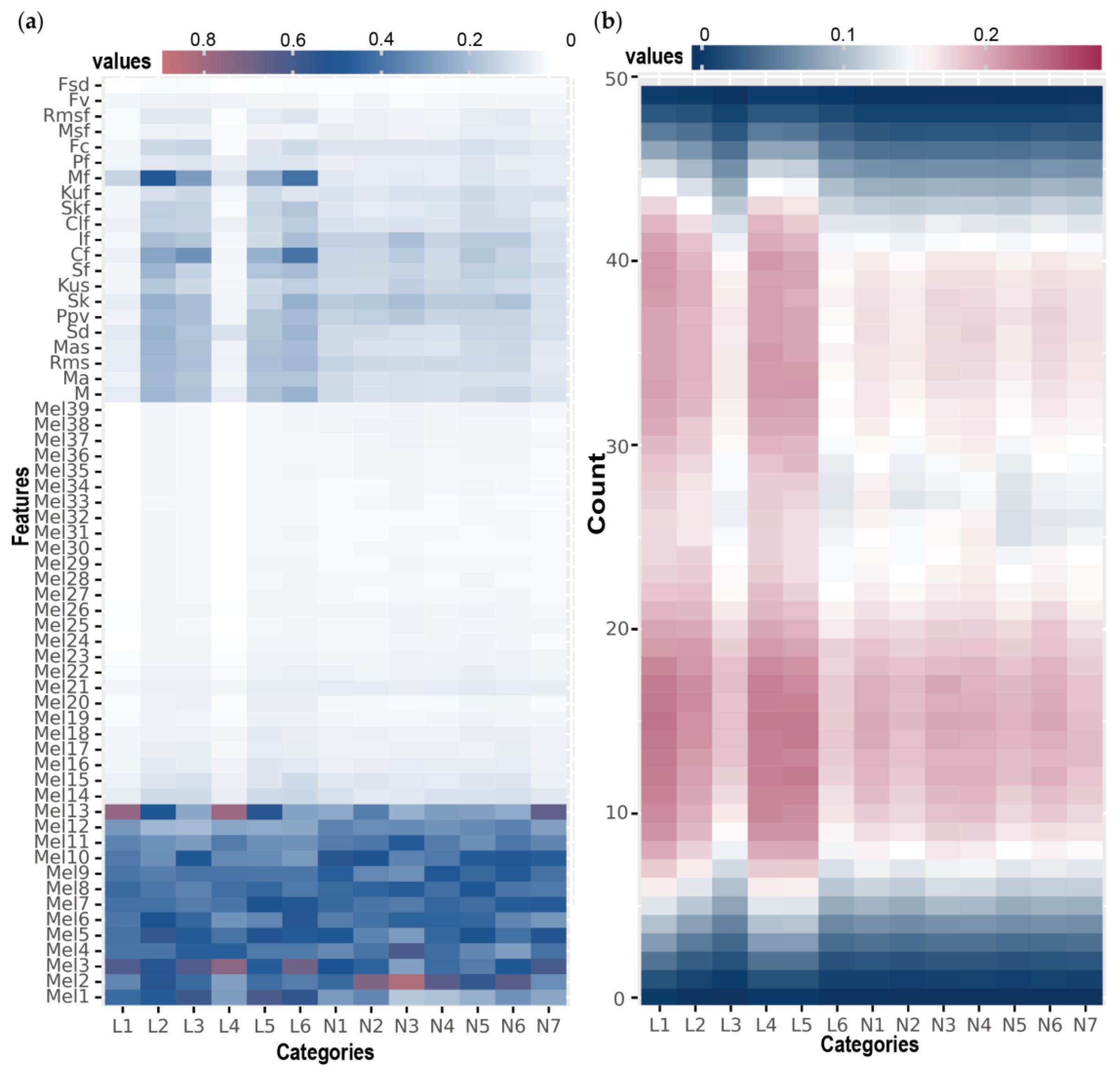
3.5. Interpretability Analysis

It is important to show what the PCNN model learned from the raw signals and handcrafted features. Saliency maps are used to visualize the impact of inputs on model predictions. To highlight important features or signal points, normalization is performed on the saliency values of each input.

Figure 16a,b show each sample category and the averaging of saliency values for handcrafted features and raw signals, respectively. The aim of averaging is to identify the common pattern for each category that the PCNN leverages to make predictions.

Figure 16a shows the PCNN has different attention patterns for leak and non-leak samples when the handcrafted features are used as input. It can be observed that that the features from $X_{Mel1}$ to $X_{Mel13}$, the clearance factor $X_{Cf}$, the margin factor $X_{Mf}$ have higher saliency values, indicating that these features are more critical to decision-making. Some categories pay additional attention to certain features, which reveals the basis for the ability of the proposed model to identify these categories. For example, $X_{Mel13}$ is the feature that the PCNN model pays the most attention to when identifying categories L₁ and L₄ as leaks. The feature $X_{Mel13}$ reflects the energy of the signal. Acoustic emission signals generated by leaks carry a substantial amount of energy [67]. The lower buried depth of leak categories L₁ and L₄ results in less attenuation in energy. Environmental noise N₇ is also observed to have a higher saliency value in $X_{Mel13}$, which may explain why some samples of N₇ were mistaken for leaks.

Figure 16a also shows that the leak categories L₂, L₃, L₅, and L₆ are more likely to focus on TFD features and dynamic MFCCs than non-leak categories. However, categories L₁ and L₄ seem to be similar to the non-leak categories. The result is consistent with the aggregation state of categories L₁, L₄, and non-leak categories in Figure 15h.

Figure 16b shows that the PCNN exhibits similar attention patterns for leak samples (except for categories L₃ and L₆) in the saliency maps for raw signals. Leak categories L₃ and L₆ show a large difference from other leak categories due to the strong signal attenuation recorded at deeper burial depths. Figure 16b also shows that all saliency maps have lower values at the top and bottom of the vertical axis. This indicates that the PCNN pays less attention to the starting and ending regions of the raw signals.

4. Conclusions

In conclusion, this study presents a novel approach for leak detection in water distribution systems (WDS) using ground acoustic signals. By integrating a PCNN structure with handcrafted features and deep representations, the authors achieve a superior performance in leak detection. The dataset was collected using electronic amplified listening devices. Additionally, the authors use four evaluation metrics and confusion matrices to assess the effectiveness of different leak detection architectures and methods.

Through optimizing the architectures and hyperparameters, the study demonstrates that the structure and hyperparameters have a significant impact on the performance of PCNN models, and that using large kernels is particularly advantageous for CNNs or PCNNs with raw acoustic signals as input.

Remarkably, the optimized PCNN model, which employs TFD features, MFCCs’ features, and raw signals as inputs, outperforms the HFB classifier and traditional deep learning architecture in leak detection. The use of MFCCs’ features and the architecture of feature fusion contributes to the impressive accuracy of 99.70%.

Although all PCNN structures using handcrafted features and raw signals as inputs perform better than CNNs, this study highlights the limitations of using the same input for PCNNs. The fusion of handcrafted features and deep representation is the key to the improvement in model performance.

Furthermore, the authors implement visualization and interpretability analysis of the PCNN, and demonstrate that the feature fusion stage of PCNN significantly reduces the misclassification phenomena in single convolution streams of CNNs. Additionally, the study highlights the potential of MFCC’ features over traditional TFD features for pipeline leak detection.

However, the efficiency of this method is still relatively low compared to correlation analysis method, and further work will focus on developing a multi-channel acoustic signals information fusion framework based on the PCNN model. The aim is to develop more convenient and efficient non-intrusive leak detection equipment, such as dynamic multi-probe instruments capable of automatic sampling. In addition, it will be interesting to implement a more robust deep learning workflow for leak detection in WDS. The proposed architecture for feature fusion can be applied in other research areas to integrate handcrafted features and deep representations.

References

1. Mekonnen, M.M.; Hoekstra, A.Y. Four billion people facing severe water scarcity. Sci. Adv. 2016, 2, e1500323. [Google Scholar]
2. Lai, W.W.L.; Chang, R.K.W.; Sham, J.F.C.; Pang, K. Perturbation mapping of water leak in buried water pipes via laboratory validation experiments with high-frequency ground penetrating radar (GPR). Tunn. Undergr. Space Technol. 2016, 52, 157–167. [Google Scholar]
3. Fahmy, M.; Moselhi, O. Automated Detection and Location of Leaks in Water Mains Using Infrared Photography. J. Perform. Constr. Facil. 2010, 24, 242–248. [Google Scholar]
4. Hu, Z.; Chen, B.; Chen, W.; Tan, D.; Shen, D. Review of model-based and data-driven approaches for leak detection and location in water distribution systems. Water Supply 2021, 21, 3282–3306. [Google Scholar]
5. Li, R.; Huang, H.; Xin, K.; Tao, T. A review of methods for burst/leakage detection and location in water distribution systems. Water Supply 2015, 15, 429–441. [Google Scholar]
6. Fan, H.; Tariq, S.; Zayed, T. Acoustic leak detection approaches for water pipelines. Autom. Constr. 2022, 138, 104226. [Google Scholar]
7. Hamilton, S.; Charalambous, B. Leak Detection: Technology and Implementation; IWA Publishing: London, UK, 2013. [Google Scholar] [CrossRef]
8. Butterfield, J.D.; Collins, R.P.; Beck, S.B. Influence of pipe material on the transmission of vibroacoustic leak signals in real complex water distribution systems: Case study. J. Pipeline Syst. Eng. 2018, 9, 05018003. [Google Scholar]
9. Xu, Y.; He, Q.; Liu, C.; Huangfu, X. Are micro-or nanoplastics leached from drinking water distribution systems? Environ. Sci. Technol. 2019, 53, 9339–9340. [Google Scholar] [PubMed] [Green Version]
10. Butterfield, J.D.; Meruane, V.; Collins, R.P.; Meyers, G.; Beck, S.B. Prediction of leak flow rate in plastic water distribution pipes using vibro-acoustic measurements. Struct. Health Monit. 2018, 17, 959–970. [Google Scholar]
11. Quy, T.B.; Muhammad, S.; Kim, J. A Reliable Acoustic EMISSION Based Technique for the Detection of a Small Leak in a Pipeline System. Energies 2019, 12, 1472. [Google Scholar]
12. Sato, T.; Mita, A. Leak detection using the pattern of sound signals in water supply systems. In Proceedings of the Sensors and Smart Structures Technologies for Civil, Mechanical, and Aerospace Systems 2007, San Diego, CA, USA, 19–22 March 2007; Volume 6529, pp. 816–824. [Google Scholar]
13. Stoianov, I.; Nachman, L.; Madden, S.; Tokmouline, T. Pipeneta wireless sensor network for pipeline monitoring. In Proceedings of the 6th International Conference on Information Processing in Sensor Networks, Cambridge, MA, USA, 22–24 April 2007; pp. 264–273. [Google Scholar]
14. Tariq, S.; Bakhtawar, B.; Zayed, T. Data-driven application of MEMS-based accelerometers for leak detection in water distribution networks. Sci. Total Environ. 2022, 809, 151110. [Google Scholar]
15. Terao, Y.; Mita, A. Robust water leakage detection approach using the sound signals and pattern recognition. In Proceedings of the Sensors and Smart Structures Technologies for Civil, Mechanical, and Aerospace Systems, San Diego, CA, USA, 10–13 March 2008; Volume 6932, pp. 697–705. [Google Scholar]
16. Li, S.; Song, Y.; Zhou, G. Leak detection of water distribution pipeline subject to failure of socket joint based on acoustic emission and pattern recognition. Measurement 2018, 115, 39–44. [Google Scholar]
17. Lim, J. Underground pipeline leak detection using acoustic emission and crest factor technique. In Advances in Acoustic Emission Technology; Springer: New York, NY, USA, 2015; pp. 445–450. [Google Scholar]
18. Kang, J.; Park, Y.; Lee, J.; Wang, S.; Eom, D. Novel Leakage Detection by Ensemble CNN-SVM and Graph-Based Localization in Water Distribution Systems. IEEE Trans. Ind. Electron. 2018, 65, 4279–4289. [Google Scholar]
19. Da Cruz, R.P.; Da Silva, F.V.; Fileti, A.M.F. Machine learning and acoustic method applied to leak detection and location in low-pressure gas pipelines. Clean Technol. Environ. Policy 2020, 22, 627–638. [Google Scholar]
20. Imah, E.M.; Afif, F.A.; Fanany, M.I.; Jatmiko, W.; Basaruddin, T. A comparative study on Daubechies Wavelet Transformation, Kernel PCA and PCA as feature extractors for arrhythmia detection using SVM. In Proceedings of the TENCON 2011—2011 IEEE Region 10 Conference, Bali, Indonesia, 21–24 November 2011; pp. 5–9. [Google Scholar]
21. Jin, H.; Zhang, L.; Liang, W.; Ding, Q. Integrated leakage detection and localization model for gas pipelines based on the acoustic wave method. J. Loss Prev. Process Ind. 2014, 27, 74–88. [Google Scholar]
22. Meng, L.; Li, Y.; Wang, W.; Fu, J. Experimental study on leak detection and location for gas pipeline based on acoustic method. J. Loss Prev. Process Ind. 2012, 25, 90–102. [Google Scholar]
23. Guo, G.; Yu, X.; Liu, S.; Ma, Z.; Wu, Y.; Xu, X.; Wang, X.; Smith, K.; Wu, X. Leakage Detection in Water Distribution Systems Based on Time–Frequency Convolutional Neural Network. J. Water Resour. Plan. Manag.-ASCE 2021, 147, 04020101. [Google Scholar]
24. Shukla, H.; Piratla, K. Leakage detection in water pipelines using supervised classification of acceleration signals. Autom. Constr. 2020, 117, 103256. [Google Scholar]
25. Spandonidis, C.; Theodoropoulos, P.; Giannopoulos, F.; Galiatsatos, N.; Petsa, A. Evaluation of deep learning approaches for oil & gas pipeline leak detection using wireless sensor networks. Eng. Appl. Artif. Intell. 2022, 113, 104890. [Google Scholar]
26. Li, Q.; Shi, Y.; Lin, R.; Qiao, W.; Ba, W. A novel oil pipeline leakage detection method based on the sparrow search algorithm and CNN. Measurement 2022, 204, 112122. [Google Scholar]
27. Spandonidis, C.; Theodoropoulos, P.; Giannopoulos, F. A Combined Semi-Supervised Deep Learning Method for Oil Leak Detection in Pipelines Using IIoT at the Edge. Sensors 2022, 22, 4105. [Google Scholar]
28. Zha, W.; Liu, Y.; Wan, Y.; Luo, R.; Li, D.; Yang, S.; Xu, Y. Forecasting monthly gas field production based on the CNN-LSTM model. Energy 2022, 260, 124889. [Google Scholar]
29. Loddo, A.; Di Ruberto, C. On the Efficacy of Handcrafted and Deep Features for Seed Image Classification. J. Imaging. 2021, 7, 171. [Google Scholar] [PubMed]
30. Bento, N.; Rebelo, J.; Barandas, M.; Carreiro, A.V.; Campagner, A.; Cabitza, F.; Gamboa, H. Comparing Handcrafted Features and Deep Neural Representations for Domain Generalization in Human Activity Recognition. Sensors 2022, 22, 7324. [Google Scholar] [PubMed]
31. Lin, W.; Hasenstab, K.; Moura Cunha, G.; Schwartzman, A. Comparison of handcrafted features and convolutional neural networks for liver MR image adequacy assessment. Sci. Rep. 2020, 10, 20336. [Google Scholar]
32. Galaz, Z.; Drotar, P.; Mekyska, J.; Gazda, M.; Mucha, J.; Zvoncak, V.; Smekal, Z.; Faundez-Zanuy, M.; Castrillon, R.; Orozco-Arroyave, J.R.; et al. Comparison of CNN-Learned vs. Handcrafted Features for Detection of Parkinson’s Disease Dysgraphia in a Multilingual Dataset. Front. Neuroinform. 2022, 16, 877139. [Google Scholar]
33. Hughes, L.H.; Schmitt, M.; Mou, L.; Wang, Y.; Zhu, X.X. Identifying Corresponding Patches in SAR and Optical Images With a Pseudo-Siamese CNN. IEEE Geosci. Remote Sens. Lett. 2018, 15, 784–788. [Google Scholar]
34. Li, W.; Yang, C.; Peng, Y.; Du, J. A Pseudo-Siamese Deep Convolutional Neural Network for Spatiotemporal Satellite Image Fusion. IEEE J. Sel. Top. Appl. Earth Observ. Remote Sens. 2022, 15, 1205–1220. [Google Scholar]
35. Gao, J.; Xiao, C.; Glass, L.M.; Sun, J. COMPOSE: Cross-modal pseudo-siamese network for patient trial matching. In Proceedings of the 26th ACM SIGKDD International Conference on Knowledge Discovery & Data Mining, Virtual Event, CA, USA, 6–10 July 2020; pp. 803–812. [Google Scholar]
36. Fan, J.; Yang, X.; Lu, R.; Xie, X.; Wang, S. Psiamrml: Target Recognition and Matching Integrated Localization Algorithm Based on Pseudo-Siamese Network. SSRN Electron. J. 2022. [Google Scholar] [CrossRef]
37. Li, Z.; Chen, H.; Ma, X.; Chen, H.; Ma, Z. Triple Pseudo-Siamese network with hybrid attention mechanism for welding defect detection. Mater. Des. 2022, 217, 110645. [Google Scholar]
38. Muda, L.; Begam, M.; Elamvazuthi, I. Voice recognition algorithms using mel frequency cepstral coefficient (MFCCs) and dynamic time warping (DTW) techniques. arXiv 2010, arXiv:1003.4083. [Google Scholar]
39. Lecun, Y.; Bottou, L.; Bengio, Y.; Haffner, P. Gradient-based learning applied to document recognition. Proc. IEEE 1998, 86, 2278–2324. [Google Scholar]
40. Xia, M.; Li, T.; Xu, L.; Liu, L.; de Silva, C.W. Fault Diagnosis for Rotating Machinery Using Multiple Sensors and Convolutional Neural Networks. IEEE/ASME Trans. Mechatron. 2018, 23, 101–110. [Google Scholar]
41. Zhang, W.; Li, C.; Peng, G.; Chen, Y.; Zhang, Z. A deep convolutional neural network with new training methods for bearing fault diagnosis under noisy environment and different working load. Mech. Syst. Signal Proc. 2018, 100, 439–453. [Google Scholar]
42. Sahidullah, M.; Saha, G. Design, analysis and experimental evaluation of block based transformation in MFCCs computation for speaker recognition. Speech Commun. 2012, 54, 543–565. [Google Scholar]
43. Arunsuriyasak, P.; Boonme, P.; Phasukkit, P. Investigation of deep learning optimizer for water pipe leaking detection. In Proceedings of the 2019 16th International Conference on Electrical Engineering/Electronics, Computer, Telecommunications and Information Technology (ECTI-CON), Pattaya, Thailand, 10–13 July 2019; pp. 85–88. [Google Scholar]
44. Chuang, W.; Tsai, Y.; Wang, L. Leak detection in water distribution pipes based on CNN with mel frequency cepstral coefficients. In Proceedings of the 2019 3rd International Conference on Innovation in Artificial Intelligence, Suzhou, China, 15–18 March 2019; pp. 83–86. [Google Scholar]
45. Xu, T.; Zeng, Z.; Huang, X.; Li, J.; Feng, H. Pipeline leak detection based on variational mode decomposition and support vector machine using an interior spherical detector. Process Saf. Environ. Protect. 2021, 153, 167–177. [Google Scholar]
46. Kopparapu, S.K.; Laxminarayana, M. Choice of Mel filter bank in computing MFCCs of a resampled speech. In Proceedings of the 10th International Conference on Information Science, Signal Processing and Their Applications (ISSPA 2010), Kuala Lumpur, Malaysia, 10–13 May 2010; pp. 121–124. [Google Scholar]
47. Rao, K.S.; Manjunath, K.E. Speech Recognition Using Articulatory and Excitation Source Features; Springer: New York, NY, USA, 2017. [Google Scholar]
48. Zhang, P.; He, J.; Huang, W.; Yuan, Y.; Wu, C.; Zhang, J.; Yuan, Y.; Wang, P.; Yang, B.; Cheng, K.; et al. Ground vibration analysis of leak signals from buried liquid-filled pipes: An experimental investigation. Appl. Acoust. 2022, 200, 109054. [Google Scholar]
49. Song, Y.; Li, S. Gas leak detection in galvanised steel pipe with internal flow noise using convolutional neural network. Process Saf. Environ. Protect. 2021, 146, 736–744. [Google Scholar]
50. Ding, X.; Zhang, X.; Zhou, Y.; Han, J.; Ding, G.; Sun, J. Scaling up your kernels to 31 × 31: Revisiting large kernel design in cnns. In Proceedings of the IEEE/CVF Conference on Computer Vision and Pattern Recognition, New Orleans, LA, USA, 18–24 June 2022; pp. 11963–11975. [Google Scholar]
51. He, K.; Zhang, X.; Ren, S.; Sun, J. Delving deep into rectifiers: Surpassing human-level performance on imagenet classification. In Proceedings of the IEEE International Conference on Computer Vision, Santiago, Chile, 7–13 December 2015; pp. 1026–1034. [Google Scholar]
52. Dozat, T. Incorporating Nesterov Momentum into Adam. ICLR 2016 workshop submission. OpenReview.net. 2016. Available online: https://openreview.net/forum?id=OM0jvwB8jIp57ZJjtNEZ (accessed on 1 February 2023).
53. Li, L.; Xu, W.; Yu, H. Character-level neural network model based on Nadam optimization and its application in clinical concept extraction. Neurocomputing 2020, 414, 182–190. [Google Scholar]
54. Fushiki, T. Estimation of prediction error by using K-fold cross-validation. Stat. Comput. 2011, 21, 137–146. [Google Scholar]
55. Krug, A.; Ebrahimzadeh, M.; Alemann, J.; Johannsmeier, J.; Stober, S. Analyzing and Visualizing Deep Neural Networks for Speech Recognition with Saliency-Adjusted Neuron Activation Profiles. Electronics 2021, 10, 1350. [Google Scholar] [CrossRef]
56. Van der Maaten, L.; Hinton, G. Visualizing Data using t-SNE. J. Mach. Learn. Res. 2008, 9, 11. [Google Scholar]
57. Simonyan, K.; Vedaldi, A.; Zisserman, A. Deep Inside Convolutional Networks: Visualising Image Classification Models and Saliency Maps. arXiv 2013, arXiv:1312.6034. [Google Scholar]
58. Arora, S.; Hu, W.; Kothari, P.K. An analysis of the t-sne algorithm for data visualization. In Proceedings of the Conference on Learning Theory, Stockholm, Sweden, 5–9 July 2018; pp. 1455–1462. [Google Scholar]
59. Cai, T.T.; Ma, R. Theoretical Foundations of t-SNE for Visualizing High-Dimensional Clustered Data. arXiv 2021, arXiv:2105.07536. [Google Scholar]
60. Gong, W.; Chen, H.; Zhang, Z.; Zhang, M.; Wang, R.; Guan, C.; Wang, Q. A Novel Deep Learning Method for Intelligent Fault Diagnosis of Rotating Machinery Based on Improved CNN-SVM and Multichannel Data Fusion. Sensors 2019, 19, 1693. [Google Scholar] [CrossRef] [Green Version]
61. Yang, D.; Hou, N.; Lu, J.; Ji, D. Novel leakage detection by ensemble 1DCNN-VAPSO-SVM in oil and gas pipeline systems. Appl. Soft. Comput. 2022, 115, 108212. [Google Scholar]
62. Hanin, B.; Sellke, M. Approximating continuous functions by relu nets of minimal width. arXiv 2017, arXiv:1710.11278. [Google Scholar]
63. Zhang, W.; Peng, G.; Li, C.; Chen, Y.; Zhang, Z. A New Deep Learning Model for Fault Diagnosis with Good Anti-Noise and Domain Adaptation Ability on Raw Vibration Signals. Sensors 2017, 17, 425. [Google Scholar] [CrossRef] [PubMed] [Green Version]
64. Xie, Y.; Xiao, Y.; Liu, X.; Liu, G.; Jiang, W.; Qin, J. Time-Frequency Distribution Map-Based Convolutional Neural Network (CNN) Model for Underwater Pipeline Leakage Detection Using Acoustic Signals. Sensors 2020, 20, 5040. [Google Scholar] [CrossRef]
65. Li, Z.; Zhang, H.; Tan, D.; Chen, X.; Lei, H. A novel acoustic emission detection module for leakage recognition in a gas pipeline valve. Process Saf. Environ. Protect. 2017, 105, 32–40. [Google Scholar] [CrossRef] [Green Version]
66. Zhang, H.; Li, Z.; Ji, Z.; Bi, Z. Intelligent leak level recognition of gas pipeline valve using wavelet packet energy and support vector machine model. Insight-Non-Destr. Test. Cond. Monit. 2013, 55, 670–674. [Google Scholar] [CrossRef]
67. Papastefanou, A.S.; Joseph, P.F.; Brennan, M.J. Experimental Investigation into the Characteristics of In-Pipe Leak Noise in Plastic Water Filled Pipes. Acta Acust. United Acust. 2012, 98, 847–856. [Google Scholar] [CrossRef]
Figure 1. Mel filters and the average MFCCs’ features’ responses: (a) The triangular filter banks with Mel frequency. The number of filter banks is 24; (b) The average value of original MFCCs’ features for leak and non-leak signals; (c) The same as (b), but using the first-order derivative of MFCCs’ features; (d) The same as (b), but using the second-order derivative of MFCCs’ features.
Water 15 01088 g001
Figure 2. Time waveforms and frequency spectra of signals for an actual leaking plastic pipe and the same pipe after repair: (a) Signal waveform; (b) Frequency spectra.
Water 15 01088 g002
Figure 3. The architecture of the PCNN. The PCNN consists of two convolutional structures in parallel for processing inputs with different scales, a convolutional structure with residual connection for feature fusion, and a two-layer multi-layer perceptron for classification. The convolution filters and inputs of the model are in one dimension.
Water 15 01088 g003
Figure 4. In situ signals’ acquisition on the ground in WDS: (a) Schematic diagram of the leak signal collection by electronic listening devices; (b) Site photo of the signal collection above a cast iron pipe with a leak. Piezoelectric ceramic probes of PQWT-LDC are used for signal collection. The direction of the pipeline is indicated by the red line with the arrow; (c) Leak hole of the cast iron pipe after excavation.
Water 15 01088 g004
Figure 5. The architectures and layer configurations for the reference convolutional neural networks: (a) Handcrafted features as input; (b) Raw signals as input.
Water 15 01088 g005
Figure 6. The architecture and layer configuration for the reference PCNN model. Hyperparameters in the feature engineering and extraction stages have been optimized based on the reference models in Figure 5a and Figure 5b, respectively. The black triangles indicate the direction of the convolution flow.
Water 15 01088 g006
Figure 7. Average confusion matrix. Sub-figures (af) correspond to models 1-6 in Table 4, respectively.
Water 15 01088 g007
Figure 8. Average confusion matrix. Sub-figures (af) correspond to models 7-12 in Table 4, respectively.
Water 15 01088 g008
Figure 9. Average confusion matrices for models 1–8 in Table 5. Sub-figures (ah) provide the corresponding visualizations for each model.
Water 15 01088 g009
Figure 10. Average confusion matrices for models 9–16 in Table 5. Sub-figures (ah) provide the corresponding visualizations for each model.
Water 15 01088 g010
Figure 11. Average confusion matrices for models 1–5 in Table 6, each represented by its corresponding sub-figure (ae).
Water 15 01088 g011
Figure 12. The training process of the PCNN showing (a) the loss; and (b) the accuracy. The dashed line indicates the epochs of early stopping.
Water 15 01088 g012
Figure 13. Average confusion matrix. Sub-figures (ag) correspond to models 1–7 in Table 7, respectively.
Water 15 01088 g013
Figure 14. Average confusion matrices for models 1-8 in Table 8, each represented by its corresponding sub-figure (ai).
Water 15 01088 g014
Figure 15. The feature map distributions of the test set derived from the input layers and inner layers of the PCNN model via the t-SNE method: (ad) Feature map distributions in the feature extraction stage; (eh) distributions in the feature engineering stage; (ik) distributions in the feature fusion stage; (l) distributions in flatten layer; and (m,n) distributions in the classification stage. The black circles in (d,h) indicate the aggregation of leak and leak samples, while that in (n) indicates the misclassifications.
Water 15 01088 g015
Figure 16. Saliency map of PCNN: (a) Saliency map for the input handcrafted features; (b) Saliency map for the input raw signals. The saliency value of each raw signal sample is averaged over every 80 points. Then, the category mean values were used to reflect the important regions for leak identification.
Water 15 01088 g016