
Impacts of Solar Radiation Management on Hydro-Climatic Extremes in Southeast Asia

1
GeoInformatic Unit, Geography Section, School of Humanities, Universiti Sains Malaysia, Penang 11800, Malaysia
2
School of Geographical Sciences, Nanjing Normal University, Nanjing 210023, China
3
Department of Earth Sciences and Environment, Faculty of Science and Technology, Universiti Kebangsaan Malaysia, Bangi 43600, Malaysia
4
Centre for Disaster Mitigation and Climate Change, Institut Teknologi Sepuluh Nopember, Surabaya 60111, Indonesia
5
Department of Statistics, Institut Teknologi Sepuluh Nopember, Surabaya 60111, Indonesia
6
Faculty of Environment and Natural Resources, Nong Lam University—Ho Chi Minh City, Ho Chi Minh City 700000, Vietnam
7
Center for Technology Business Incubation, Nong Lam University—Ho Chi Minh City, Ho Chi Minh City 700000, Vietnam
8
College of Geography and Environmental Sciences, Zhejiang Normal University, Jinhua 321004, China
9
College of Geography and Remote Sensing Sciences, Xinjiang University, Urumqi 830017, China
*
Author to whom correspondence should be addressed.
Water 2023, 15(6), 1089; https://doi.org/10.3390/w15061089
Submission received: 11 February 2023
/
Revised: 6 March 2023
/
Accepted: 9 March 2023
/
Published: 13 March 2023
(This article belongs to the Section Water and Climate Change)
Abstract
:Solar radiation management (SRM), or solar geoengineering, reduces the earth’s temperature by reflecting more sunlight back to space. However, the impacts of SRM remain unclear, making it difficult to project the benefits as well as consequences should this approach be adopted to combat climate change. To provide novel insight into the SRM impact on hydro-climatic extremes in Southeast Asia, this study conducts a simulation experiment for the Kelantan River Basin (KRB) in Malaysia by incorporating three bias-corrected Stratospheric Aerosol Geoengineering Large Ensemble (GLENS) members into the Soil and Water Assessment Tool Plus (SWAT+) model. The study found that SRM practices could generate substantial cooling effects on regional temperatures, leading to a reduction in projected annual precipitation and monthly precipitation during the flooding season (from November to mid-January) under SRM relative to the Representative Concentration Pathway 8.5 (RCP8.5) scenario. In addition, SRM could reduce the number of days with heavy precipitation as well as the intensity of maximum daily precipitation as compared to RCP8.5, during the 2045–2064 and 2065–2084 periods, leading to a reduction in high flows. Nevertheless, under SRM impacts, the driest months from February to May would experience comparable decreases in monthly precipitation and streamflow.
Keywords:
climate change; solar radiation management; geoengineering; hydrology; flood; SWAT+; Malaysia1. Introduction
Anthropogenic climate change presents a significant threat to global socio-economic, ecological, and environmental systems and endangers human life [1]. Changing climatology and extremes of the earth’s climate system are anticipated to lead to more intense natural hazards [2,3], which could collectively cause about 260 to 360 billion dollars in economic losses every year [4]. In a warming climate, the atmosphere is able to hold more moisture, leading to intensifying extreme rainfall events [5], and ultimately higher flood hazards in many regions of the world [6,7]. Floods occur in different places and have multi-dimensional impacts on the global and local economy [8]. Therefore, local-scale adaptation measures, which integrate flood protection embankment development and wetland and forest restoration, as well as risk finance mechanisms, are required to effectively manage and minimize flood losses [9]. In addition, many global initiatives have been proposed to slow down anthropogenic warming and the associated impacts of natural disasters, including floods, as reported in the Sixth Assessment Report of the Intergovernmental Panel on Climate Change (IPCC) [10].
As part of the Paris Agreement, the IPCC has emphasized the important of limiting global warming to “well below 2 °C”, and if possible, to 1.5 °C in comparison to pre-industrial levels, as a collective effort to mitigate climate change [11]. To achieve this objective, the Solar Radiation Management (SRM) concept, also called solar geoengineering, has been proposed to mitigate climate change by reflecting more sunlight back to space and ultimately lowering the earth’s temperature [12,13]. Stratospheric aerosol injection (SAI), marine cloud seeding, and sunshades in space are three potential SRM techniques to reflect the incoming sunlight for providing global and regional cooling [14]. However, SRM is a controversial concept, as its technologies might bring advantages to some regions of the world but more hazards in others. Understanding of the global and local impacts of SRM technologies remains limited [15], resulting in a reluctance to accept SRM by the public at large [16].
Due to widespread agreement on the impacts of anthropogenic climate change, increased scientific efforts have focused on the ability of different SRM techniques to affect future climate conditions at the global and regional scales. To minimize the impacts of SRM techniques on Earth’s systems, models have been used as the primary approach in these investigations [17] and have further allowed for confidence in SRM’s cooling effects. Tilmes et al. [18] reported that SRM can significantly reduce precipitation extreme events and evaporation amounts on global and regional levels. Similar findings of decreases in global precipitation and evaporation were reported by Dagon and Schrag [19] following consistent decreases in the top-of-atmosphere solar irradiance by 1%, 2% and 3%. However, research on SRM’s impacts on developing and less-developed countries is still limited and thus characterized with high uncertainty. For instance, using the Stratospheric Aerosol Geoengineering Large Ensemble (GLENS) experiments, Pinto et al. [20] projected decreases of mean and extreme temperatures over sub-Saharan Africa under SRM, but the precipitation changes tended to be non-linear. More recently, Kuswanto et al. [21] projected a significant reduction of mean and extreme temperatures over the Indonesian Maritime Continent after the injection of 5Tg of SO2 through SAI experiments from 2020 to 2069 in the equatorial lower stratosphere.
It is important to note that most studies have focused on the immediate effects of SRM technologies on the climate variables rather than ecosystem response [22], such as potential impacts on hydrological extremes, including floods. Wei et al. [23], Kleidon et al. [24] and Dagon and Schrag [19] were among the first to investigate SRM’s impact on hydrology, flood risk and streamflow in different parts of the world. Wei et al. [23] found that streamflow is projected to decrease in the eastern part of Eurasia and North America but increase in the western part. Although the experiment showed that SRM tended to reduce flood risk in most locations, it lacked a basin-scale modelling framework, which is crucial to provide a robust impact assessment for the detailed design of local flood control facilities.
To date, Camilloni et al. [25] are the only researchers to evaluate the hydro-climatic response of the La Plata Basin by incorporating GLENS into the Variable Infiltration Capacity (VIC) hydrological model. They found that SRM is able to reduce not only the extreme precipitation and temperature but also floods when compared to hydrological simulations forced by climate projections without any SRM practices involved. However, the SRM impact varies spatially and temporally due to different geographical, topographical and climate conditions [26]. As mentioned earlier, most SRM studies in hydrology have been carried out on a global scale. The effects of SRM on hydro-climatic extremes over river basins in Southeast Asia is still understudied in the literature.
In this study, the Kelantan River Basin (KRB)—a tropical basin that is frequently affected by floods in Malaysia [27,28]—was selected. To evaluate the effect of climate change on water resources in the KRB, Tan et al. [29] utilized the Soil and Water Assessment Tool (SWAT) and Coupled Model Inter-comparison Project Phase 5 (CMIP5) models. They further updated the hydro-climatic assessment using the latest CMIP6 High-Resolution Model Inter-comparison Project (HighResMIP) experiments, focusing on model resolution comparison and extreme flow analysis [30]. Both studies concluded that climate change will likely cause more frequent and intense floods in the KRB, especially under the RCP8.5 high-emission scenario. However, no research has been conducted to assess how SRM influences the changes in flood risk over the KRB, although SRM techniques could potentially reduce the mean temperature in this region [21].
Therefore, this study explores the impacts of SRM on hydro-climatic extremes in Southeast Asia, particularly floods, with the KRB as the first case study. The specific objectives include: (1) to bias-correct the GLENS data with the quantile mapping approach; (2) to calibrate and validate the newly released SWAT plus (SWAT+) model in simulating daily and monthly streamflow; and (3) to assess the hydro-climatic changes in the near (2025–2044), middle (2045–2064), and end (2065–2084) of the 21st century as compared to the baseline period (1985–2004). This is the first study to evaluate the SRM impact on hydro-climatic extremes (especially floods) in Southeast Asia at the basin level; it can provide new insights to stakeholders and policy makers, since previous SRM studies were mostly focused at the global and regional levels. This is also one of the earlier studies to apply SWAT+ in Southeast Asia, so it offers crucial information to SWAT+ developers and users. Due to practical constraints, this study does not provide a comprehensive comparison between SWAT and SWAT+ for streamflow simulations in the KRB.
2. Materials and Methods
2.1. Study Area
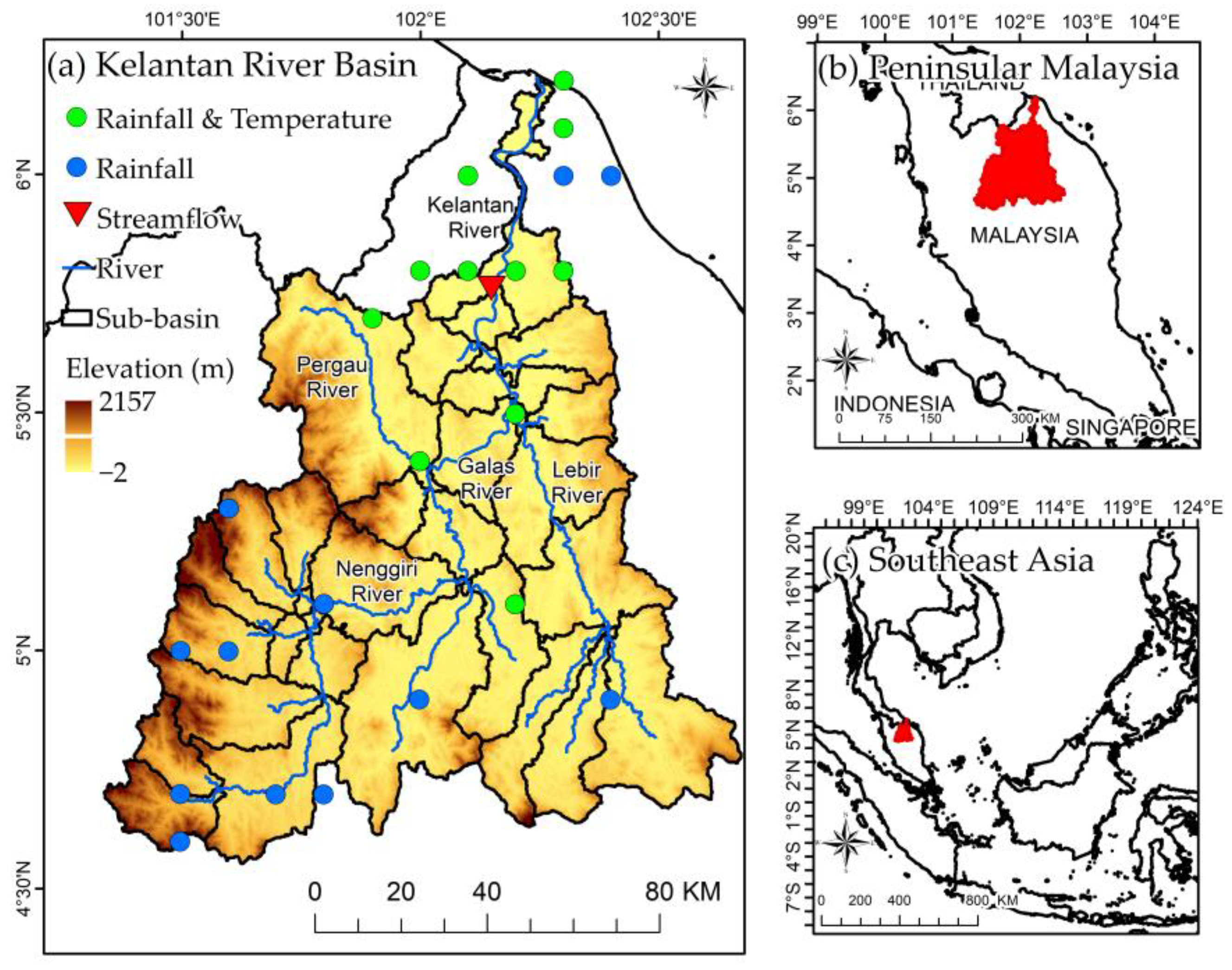
The KRB is an important basin of Malaysia; it covers about 85% of the Kelantan state and is characterized with an equatorial climate (see Figure 1). The KRB river system flows northward from the central mountain range and the Tahan mountain range to the South China Sea. Along the way, the river passes through several major towns of the Kelantan state, including Kuala Krai, Kota Bharu (the riverside capital), Tanah Merah and Pasir Mas. About 100 km from the river’s mouth, close to Kuala Krai, the Kelantan River is produced as a confluence of the Galas and Lebir Rivers. In the western part of the KRB, the Nenggiri and Pergau Rivers constitute headwaters of the Galas River (Figure 1). The basin’s topography ranges between −2 and 2157 m, where mountainous areas are mostly western, south-western, southern and south-eastern. Forest covers approximately 70.8% of the basin, while rubber and oil palm are the main crops, accounting for approximately 13.3% and 11.1% of the basin, respectively. The remaining land-use types include other agricultural, paddy and urban, at 2.9%, 1.3% and 0.6%, respectively [30].
Between 1985 and 2014, the basin received high annual precipitation amounts, ranging from 2000 mm/year to 3200 mm/year [31]. It regularly experiences drier conditions from March to May and monsoon flooding from November to January, with average maximum temperature from 29.3 to 34.1 °C and average minimum temperature from 22 to 23.8 °C [30]. The KRB was chosen as the research location due to the features of its tropical rainforest environment, which could be a valuable comparison site. In addition, the KRB is frequently affected by floods, particularly during the early phase of the Northeast Monsoon season, from November to mid-January. Another important consideration when choosing the KRB was the fact SWAT has been successfully established and utilized in the basin [32,33] to assess hydro-climatic changes under different emission scenarios, which that could be for comparison with the SRM experiments conducted in this study.
2.2. Climate Projections
The GLENS project [18] utilizes the Whole Atmosphere Community Climate Model (WACCM) together with the Community Earth System Model (CESM1) [34] to simulate the SRM effects. Under the GLENS experiments, sulphur dioxide (SO2) is concurrently injected into the stratosphere from 2020 to 2100 along 180° E at four locations of 30° S, 15° S, 15° N and 30° N. This injection occurs at a height of approximately 5 km above the height of the climatological tropopause [35]. The total SO2 injection amount will be 52 Tg SO2/year by the end of the 21st century, where about 80% of the SO2 is distributed at 30° S and 30° N, followed by 15° N, and very little at 15° S [36]. These GLENS ensemble members are simulated following the Representative Concentration Pathway 8.5 (RCP8.5) scenario, so that a comparison can be made between SRM and the “worst case” climate projection. GLENS simulation is configured to keep the global mean surface temperature, equator-to-pole surface temperature and interhemispheric temperature stable at 2020 values under the RCP8.5 scenario [36].
This study selected three ensemble members of the GLENS project, which are associated with its corresponding RCP8.5 simulations over the 2010–2097 period. In the following text, figures, and tables, the GLENS and RCP8.5 terminology was used to respectively denote the control (i.e., SRM techniques would be used to mitigate global warming) and feedback (i.e., no SRM technique would be adopted, leading to the occurrence of the usual “worst-case” climate change scenario) simulations, including hydrological application. Further information on the GLENS experiments is available in the article written by Tilmes et al. [36]; a more detailed description on data processing in this study is provided in Section 2.4.
2.3. Hydrological Model
To assess the impacts of SRM practices on hydrological extremes over the KRB, this study used SWAT+ to simulate future streamflow regimes. SWAT is a semi-distributed hydrological model that has been extensively used to investigate how land use, climate change, and different land management practices affect the quality and quantity of water resources at both the surface and underground. SWAT+, a restructured and improved version of SWAT, was specifically used, which allows additional flexibility in linking various spatial units while representing different management activities [37,38].
Compared to the previous edition, SWAT+ is more flexible in spatial representation of the interactions and processes within a river basin. It subdivides a river basin into hydrologic response units (HRUs) after dividing the river basin into sub-basins, which are linked by a stream network. HRUs are areas with similar land use, soil, slope, and management practices within a particular sub-basin [39]. In SWAT+, sub-basins can also be separated into two or more landscape units (LSUs), such as upland and flood plain areas. There will be a unique set of HRUs at each LSU because HRUs are defined following LSU delineation [37]. The flow simulated within the HRUs is aggregated at the LSU level, which could be transferred from a LSU to other spatial objects within the basin, such as wetlands, reservoirs, ponds, channels and other LSUs.
2.4. Hydro-Climatic Impact Assessment Framework
Figure 2 depicts the overall conceptual framework of this research. The data required to conduct this study can be divided into four major types: (1) Climate projections: three ensemble members of GLENS and their corresponding RCP8.5 climate projections (described in Section 2.2); (2) Geospatial data: digital elevation model (DEM), land and soil for setting up SWAT+; (3) Observed daily climate data: precipitation, maximum and minimum temperature data for bias correction of climate projections as well as to set up the SWAT+ model; and (4) Observed hydrology data: daily streamflow data needed to calibrate and validate the SWAT+ model.
Since the baseline period was set up between 1985 and 2004, the land-use map of 2006 produced by the Department of Agricultural Malaysia (DOA) was used in this study. Although land-use changes could substantially modulate hydrological changes, the 2006 land use profile was used for all simulations, as land-use change impacts are not within the scope of our study. Soil maps were obtained from the FAO-UNESCO soil map, which has been widely used in SWAT modelling around the world [30,40]. Shuttle Radar Topography Mission (SRTM) DEM was used for the basin and sub-basin delineation as well as the creation of the river network. Observed precipitation and temperature from 25 stations within and surrounding the basin, installed and operated by Malaysian Meteorological Department (MMD), as shown in Figure 1, were used to bias-correct GLENS and RCP8.5 climate simulations as well as to set up SWAT+. Daily streamflow data at the Jambatan Guillermard station, operated by the Department of Irrigation and Drainage (DID), in the downstream part of the basin were applied to calibrate and validate SWAT+. According to Tan et al. [30], the streamflow station has an average annual streamflow of 475.81 m3s−1, with high monthly streamflow found in November (781.9 m3s−1), December (1296.3 m3s−1) and January (721.3 m3s−1).
2.4.1. Bias Correction of Climate Projections
General circulation models (GCMs) usually simulate daily rainfall and temperature and are biased and skewed in their distributions [41]. To overcome this issue, prior to using GCM output to drive the hydrological model, bias-correction techniques are usually used to adjust bias and skewed distribution of the GCM output to match that of observational records. Among the bias-correction techniques, quantile mapping (QM) has been considered as one of the most reliable techniques and is extensively used in correcting GCMs and regional climate models before applying for hydrological modelling [42,43,44,45].
To adopt this approach, the quantiles with regard to the distribution of each simulated climate variable are first calculated. The observed value corresponding to each quantile is then computed based on observations. A mathematical relationship between the simulated and observed quantiles is then constructed and used to systematically correct the simulated variables.
For precipitation, multiplicative factors are usually calculated from the modelled (Psim) and the observed precipitation (Pobs) for similar quantiles from the two distributions, as described in Equation (1).
where r indicates the r-th quantile under consideration. The factors Fr for rainfall and FT for temperature were then used to modify the GCM simulated output for similar quantiles outside the reference period to produce bias-corrected precipitation (), following Equation (2).
For temperature, an additive factor is used instead to generate bias-corrected temperature (T′sim), as described in Equations (3) and (4).
FT = Tobs(r) − Tsim(r)
T′sim (r) = Tsim(r) + FT
Instead of pre-fitting the data using a parametric distribution, this approach determines the quantile values directly from the empirical distribution. When compared to parametric methods, non-parametric methods often yield superior results [2]. In this study, the QM method was applied to both GLENS and RCP8.5 climate datasets to eliminate the systematic bias of these projections. More information on the QM method can be obtained from Ngai et al. [46].
2.4.2. Hydrological Modelling
In this study, the latest SWAT+ rev 60.5.4 version that was compatible with the QGIS 3.22 software was used. The QSWAT+ 2.2.3 tool was installed as a plug-in to QGIS as an interface to set up the model. Basically, there are four major steps in setting up the model: (1) watershed delineation; (2) HRU creation; (3) editing of inputs and running SWAT+; and (4) visualizing the results. In the watershed delineation, the minimum channel threshold was set to 200 km2, which resulted 36 sub-basins for the KRB. In the HRU creation, the slope bands were divided into five classes of 0–10%, 10–20%, 20–30%, 30–40% and above 40%. In addition, the HRUs were filtered by the threshold of 10% for each slope, soil and land use, which created 443 HRUs. The SWAT+ Editor 2.1 was incorporated in step 3 to edit SWAT+ inputs and run for the 1980–2004 period, with a warm-up phase of the initial five years.
A free tool called SWAT+ Toolbox v1.0 enables SWAT+ users to conduct sensitivity analysis, calibration and validation [47]. As mentioned previously, daily discharge data from 1985 to 2004 at the Jambatan Guillemard was applied to calibrate and validate SWAT+. The Delta Moment-Independent Measure was used, with 500 runs to check the sensitivity level of different parameters in the streamflow simulation of the KRB. An automatic calibration first ran 500 rounds using the Dynamically Dimensioned Search (DDS) method with maximized Nash-Sutcliffe Efficiency (NSE) set at the objective function. Similarly, Tan et al. [29] reported NSE as the optimal objective function for the SWAT simulation in the KRB as compared to Coefficient of Determination (R2), adjusted R2, Percentage Bias (PB) and sum of the squares of residuals (SSQR). Then, the ideal parameter values were entered manually via the hard calibration function in the SWAT+ Editor 2.1 tool. The SWAT+ model was further calibrated manually to adjust the parameters based on the basin characteristic in order to achieve optimal performance. The most popular statistical methods for evaluating the SWAT’s performance are the R2, NSE, and PB [48]. The ideal value for R2 (0 to 1) and NSE (−∞ to 1) statistical metrics is 1, while for the PB it is 0. According to Moriasi et al. [49], the capability of SWAT+ to simulate daily or monthly streamflow should be regarded as acceptable if the R2, NSE and PB values are more than 0.6, 0.5 and ±15%, respectively.
2.4.3. Hydro-Climatic Modelling
Six bias corrected climate projections, i.e., three GLENS (control simulations) and three RCP8.5 (feedback simulations) ensembles, were used to simulate the hydro-climatic pattern via the calibrated SWAT+ model for the baseline (1985–2004) and three future periods: near (2025–2044), middle (2045–2064) and end (2065–2084) of the 21st century. Then, analysis of the differences between future simulations relative to the baseline simulations was conducted to understand potential changes in hydro-climatic extremes under different climate scenarios. The following variables were used to assess hydro-climatic changes across the basin.
- The 20-year mean of annual temperature, precipitation and streamflow were used to assess changes in climatological conditions across the basin.
- The Expert Team of Climate Change Detection Indices (ETCDDI) [50] were then used for climatic extreme analysis, specifically focused on the common flood-related indices: the number of precipitation days with greater than 10 mm/day (R10 mm), 20 mm/day (R20 mm), 50 mm/day (R50 mm) and annual maximum daily rainfall amount (Rx1d).
3. Results
3.1. Bias-Corrected Climate Projections
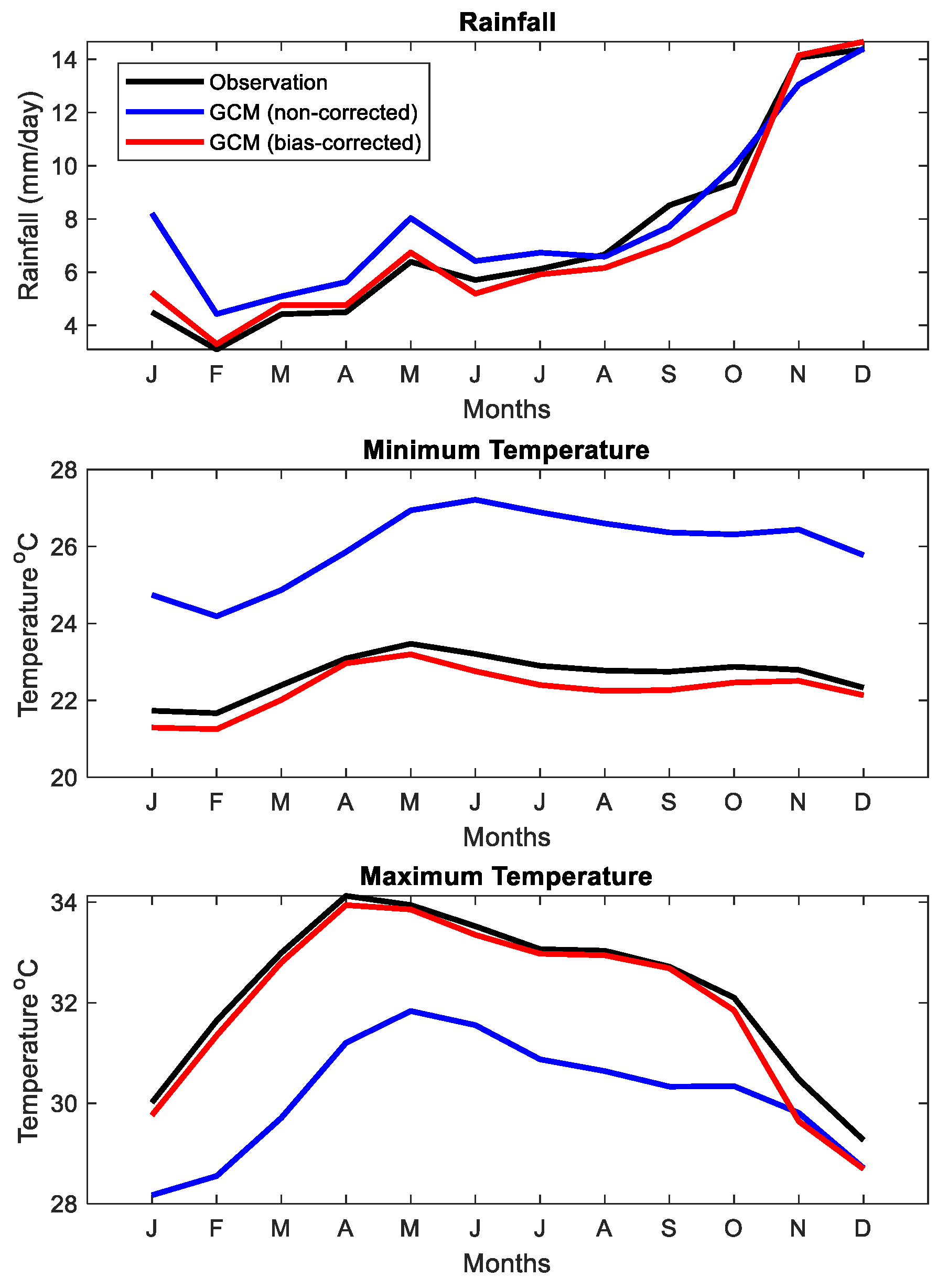
Figure 3 shows the climatological comparison between the station observations averaged over the entire Kelantan catchment and the raw GLENS simulations and the bias-corrected GLENS output. It is noted that the GLENS simulation produced the precipitation climatology correlated well, despite some over-estimation during the first half of the year. The rainfall peak in November and December as well as the dry period in February is well captured by GLENS. The bias correction generally rectified the wet biases from January to July but resulted in slightly drier climates in September and October. Overall, the bias correction on the precipitation achieved an improvement of spatial mean absolute error from 0.97 to 0.21 mm/day (Table 1).
The surface temperature simulation of GLENS tended to have remarkable biases throughout the year. Specially, it underestimated maximum temperature (cold biases) and overestimated minimum temperature (warm biases). This indicates that GLENS tends to simulate a much lower diurnal temperature range (DTR) as compared to the observations. A few reasons may contribute to the lower DTR in the GLENS simulation. The observations of temperature at stations are relatively instantaneous, while GCM-simulated minimum and maximum temperature were averaged over a time step in the climate models, causing the temperature biases toward lower DTR [51]. Another potential factor in lowering the DTR in the simulation is the overestimation of clouds cover [52]. More clouds in the atmosphere prohibit incoming solar radiation to the Earth during the daytime and prohibit outgoing long-wave radiation at night into space, result in the systematic biases (cold and warm) in the maximum and minimum temperatures. When computed across the stations, the mean absolute errors of the raw GLENS-simulated maximum temperature and minimum temperature are 2.1 °C and 3.3 °C, respectively. These performance metrics are improved to 0.27 °C and 0.3 °C (Table 1), respectively, when the GLENS simulations were bias-corrected.
3.2. Climatic Changes
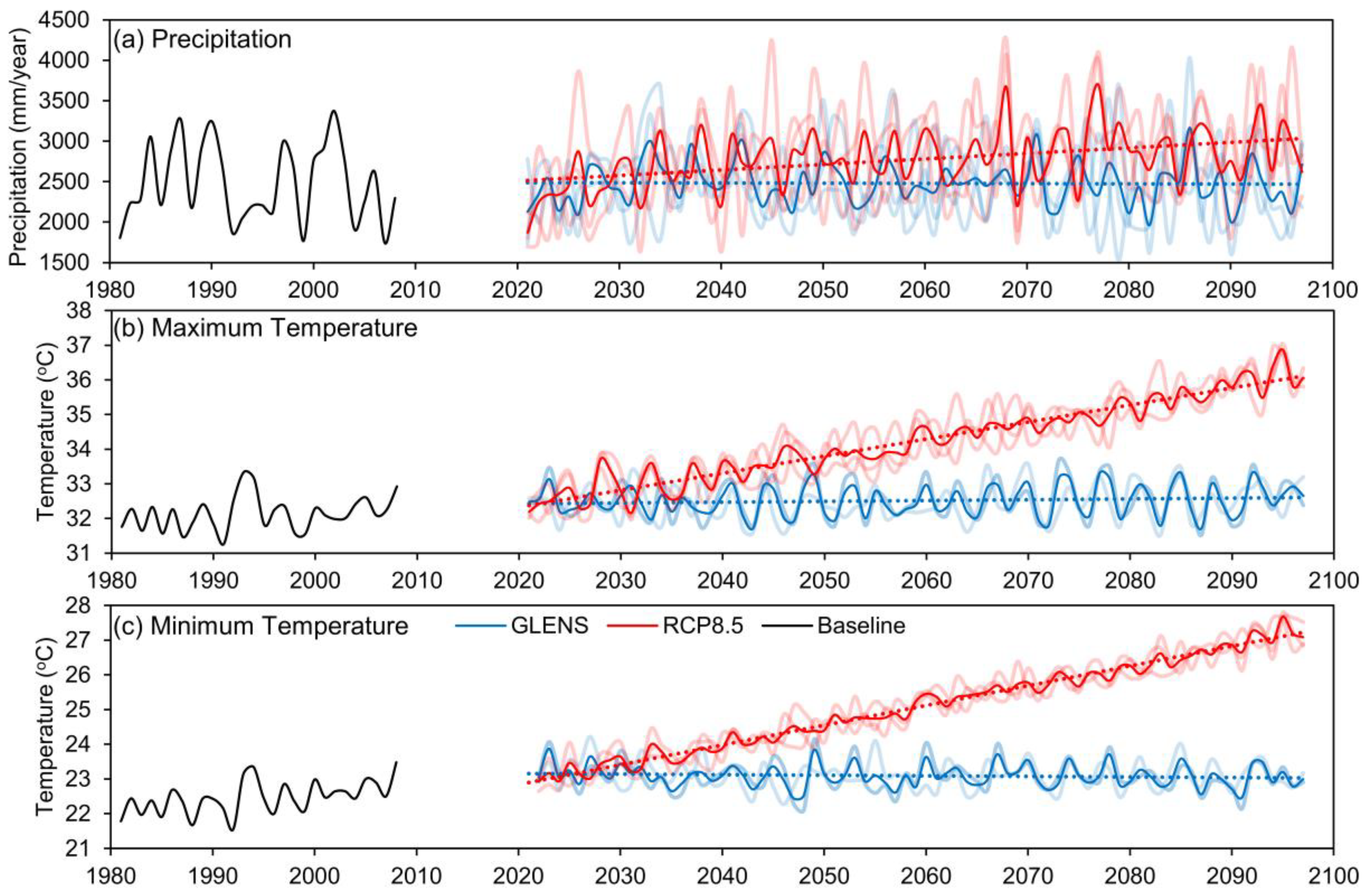
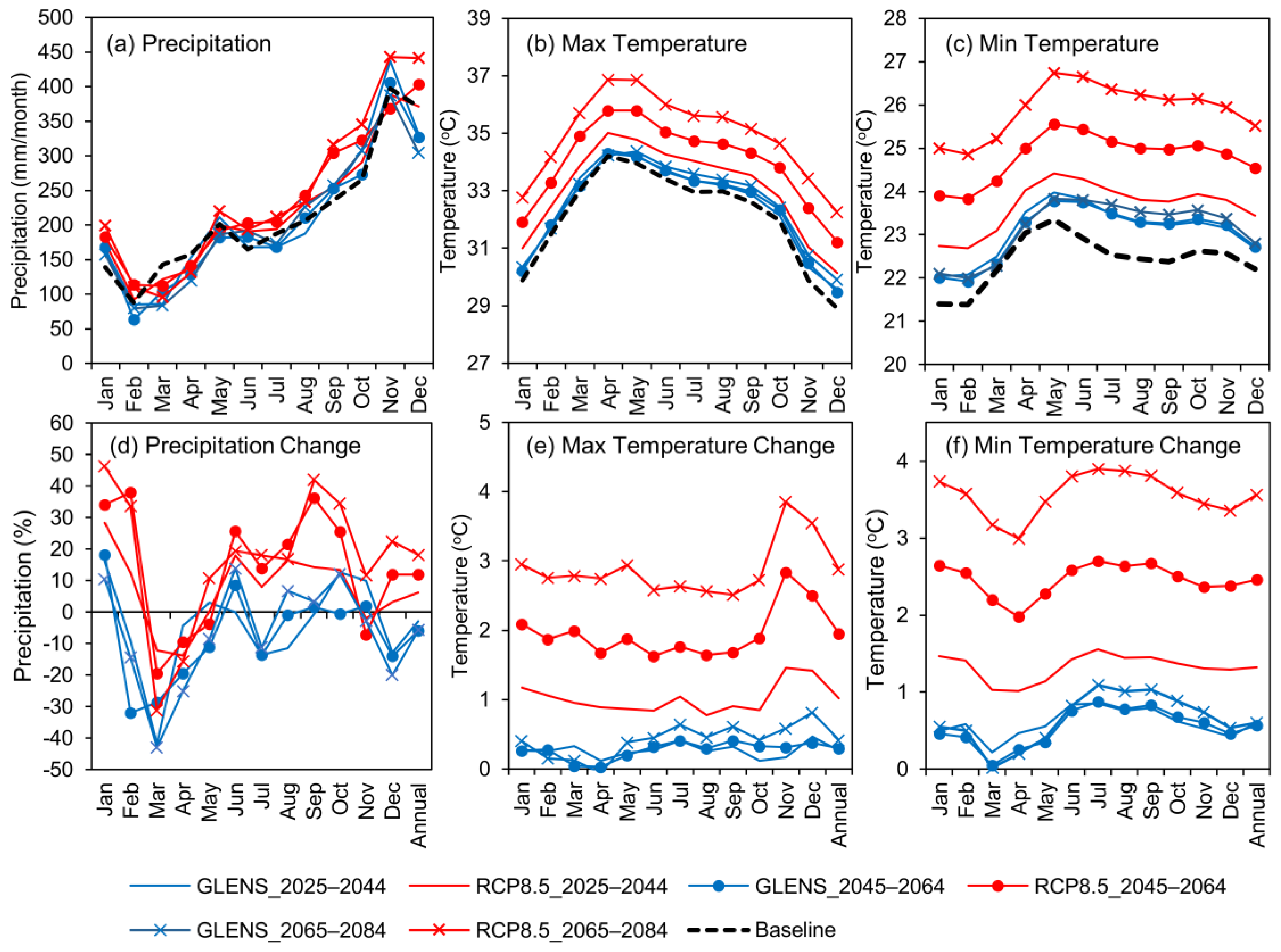
The evolution of climatic changes for annual total precipitation and annual mean maximum and minimum temperatures over the KRB from 1981 to 2097 under both the RCP8.5 and GLENS simulations are illustrated in Figure 4. RCP8.5 was chosen because of its high signal-to-noise ratio, which is beneficial for evaluating climatic response in comparison with GLENS [26]. GLENS simulations show that precipitation over the KRB would typically become less intense under SRM than RCP8.5, offsetting the positive force from the rising GHG concentration. For instance, the increases of annual total precipitation by 6.26% to 18.08% under RCP8.5 could be offset by GLENS, where annual total precipitation was projected to decrease by 2.87% to 6%, as illustrated in Figure 5a,b. A similar offset situation is found in the monthly precipitation simulations, particularly in the early northeast monsoon season (November to January), the flooding period in Malaysia as indicated in Figure 5d. The decreases of monthly precipitation under SRM could be helpful to reduce the risk of flooding in the basin. However, similar decreases in monthly precipitation can also be found during the dry season from February to May, showing that SRM may intensify the water scarcity issue in Kelantan.
It is noted that there is remarkable cooling of mean minimum and maximum temperatures under GLENS compared to RCP8.5, as shown in Figure 4 and Figure 5. Annual mean maximum temperature in the GLENS simulation is comparable to the historical level, which is projected to increase marginally, by 0.26, 0.29 and 0.42 °C for the 2025–2044, 2045–2064 and 2065–2084 periods, respectively. By contrast, under RCP8.5, the annual mean maximum temperature of the KRB is projected to rise significantly, by 1.02, 1.96 and 2.88 °C during the periods of 2025–2044, 2045–2064 and 2065–2084, respectively. However, compared to historical simulation, the mean minimum temperature of GLENS simulation is still substantially higher (annual = 0.6) than the historical simulations. Therefore, the reduction of mean minimum temperature is not as drastic as the mean maximum temperature. The increase in stratospheric aerosols decreases the downward longwave and shortwave radiation fluxes [53]. The increase in the stratospheric aerosol can have a profound effect on the cloud properties. Using the Geoengineering Model Intercomparison Project (GeoMIP) G1 experiment, Russotto and Ackerman [54] showed that the increase in stratospheric aerosols may increase cloud cover. This could reduce the outgoing longwave radiation and increase downward longwave radiation, therefore offsetting the effect of the drastic cooling achieved during day time.
3.3. Climatic Extremes Changes
Precipitation extreme indices that are closely related to the occurrences of flood events, R10 mm, R20 mm, R50 mm and Rx1d, were used for the analysis of SRM impact on climatic extremes. Under RCP8.5, the R10 mm, R20 mm and R50 mm indices are projected to increase across the basin by 0.9–11.93%, 2.8–21.64% and 6.41–97.8%, as illustrated in Figure 6. Figure 7 shows that the R10 mm, R20 mm and R50 mm values are higher under RCP8.5 as compared to GLENS for all the three evaluated periods. R50 mm is projected to increase significantly in the south-western and middle parts, up to double the number of days in the 2065–2084 period compared to the baseline period (Figure 6). Meanwhile, under GLENS, the magnitude of the R10 mm, R20 mm and R50 mm changes is greatly reduced and comparable to the historical period, showing SRM can effectively reduce the number of extreme precipitation days in the KRB as compared to RCP8.5.
During the 2025–2044 period, the Rx1d values under the GLENS and RCP8.5 simulations are similar, ranging from 96.4 to 236.8 mm/day and 99.57 to 217.05 mm/day, respectively, as demonstrated in Figure 7d. In terms of spatial changes, Rx1d slightly increases across the basin under both the GLENS and RCP8.5 simulations in the 2025–2044 period, as shown in Figure 6. Interestingly, Rx1d tends to increase up to 25.38% and 48.16% under RCP8.5 for both the 2045–2066 and 2065–2084 periods, respectively. Meanwhile, the magnitude of changes in Rx1d is weaker under GLENS in the mid- and late-21st century when compared to RCP8.5. Similar to R50 mm, the dramatic increases of Rx1d in the south-western and middle parts of the basin under RCP8.5 in the 2065–2084 period can be effectively offset by SRM, as illustrated in Figure 6.
3.4. SWAT+ Calibration and Validation
Maximum canopy storage (CANMX), soil evaporation compensation coefficient (ESCO), lateral flow coefficient (LATQ_CO) and curve number condition II (CN2) are the most sensitive parameters for daily streamflow simulations using SWAT+ in the KRB, as listed in Table 2. CN2 is commonly known as a highly sensitive parameter in SWAT modelling, not only in this study [30] but also for other river basins [40,55]. As the default SWAT+ model simulated higher surface and base flows than reality, the CN2 values were reduced to lower the surface runoff and soil infiltration to replicate the hydrological cycle of tropical forest that dominates in the basin. CANMX refers to the maximum amount of water that can be kept in the trunk or canopy; this plays a vital role in controlling the infiltration, evapotranspiration and surface runoff in tropical regions [56]. The CANMX value was set 80 to represent the tropical rainforest conditions of the basin.
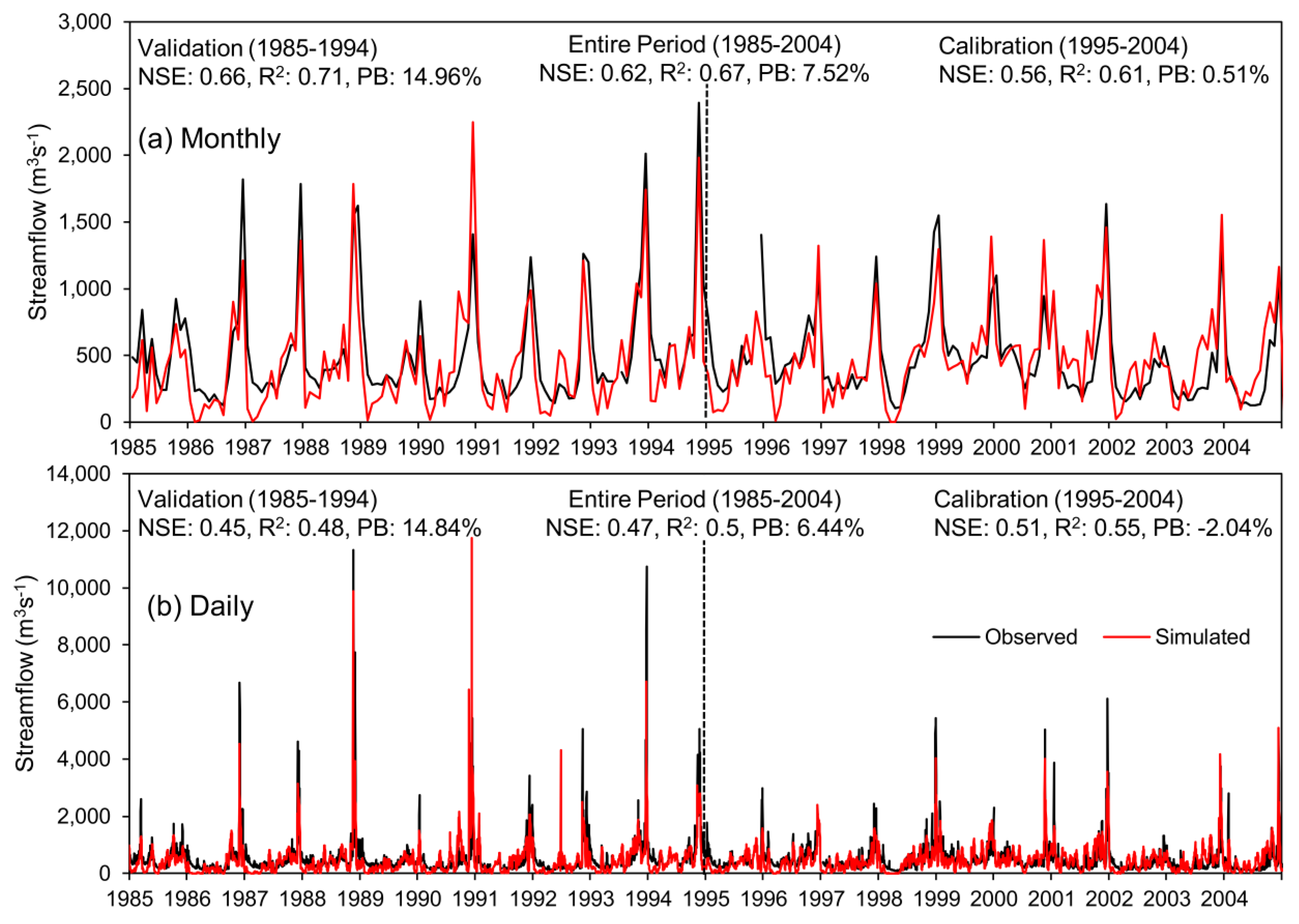
The selection of objective function has an effect on the calibration and validation of a hydrological model [57]. To solve this problem, this study utilized both manual and automatic calibration procedures for the SWAT+ modelling in the KRB. Figure 8 indicates the SWAT+ simulated flows and observed flows at the Jambatan Guillermard station between 1985 and 2004 for both monthly and daily time scales. The R2 and NSE values are generally greater than 0.5, with the RB values within 15%, indicating the SWAT+ model can adequately capture the variability flows for both the monthly and daily scales. In daily simulation, the performance for the validation period is slightly poorer than for the calibration period; nonetheless, it is still acceptable based on Moriasi et al. [49]. This is quite a common result, since the parameter values were tested mainly based on the calibration period. Figure 8 shows that SWAT+ tended to underestimate the peak flows; similar findings were reported in previous SWAT studies in tropical regions [58,59]. This may be due to the lack of well-distributed and good-quality climate data for the model development, particularly in the middle, eastern and south-eastern parts of the basin, as shown in Figure 1 [30]. In addition, the modules within SWAT+ were developed mainly based on conditions in the United States, which might not perfectly represent the tropical hydrological cycle. However, the statistical metrics indicate that the SWAT+ model is sufficiently reliable for the following analysis.
3.5. Hydrological Changes
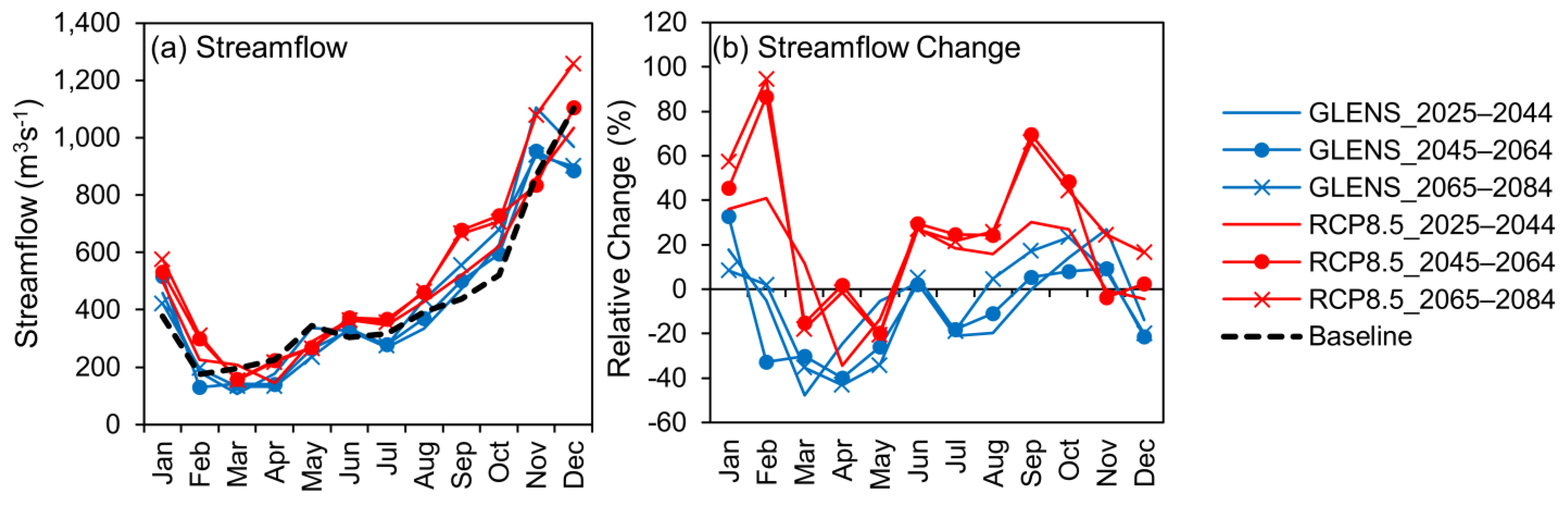
Monthly streamflow projection at the Jambatan Guillermard for the 2025–2044, 2045–2064 and 2065–2084 periods and the 1985–2004 baseline period under the GLENS and RCP8.5 simulations is shown in Figure 9. It is projected that monthly streamflow would increase significantly in January by 8.38 to 32.68% under GLENS and by 35.96 to 57.28% under RCP8.5. In December, monthly streamflow is projected to vary by −4.29 to 16.52% under RCP8.5 and to decrease by 13.92 to 19.94% under GLENS, showing SRM can effectively reduce monthly flows during the flooding period of December and January as compared to RCP8.5.
By constrast, monthly streamflow in March, April and May, the driest months in the basin, is projected to further decrease under GLENS by 30.07 to 47.81%, 24.49% to 43.06% and 5.43 to 34.09%, respectively (Figure 9). During the south-west monsoon season, RCP8.5 may result in increases in monthly streamflow, while GLENS reduces the magnitude changes significantly, particularly in July, August and and September. Previous hydro-climatic modelling studies reported that the wet season of the KRB will become wetter, and the dry season will become drier [29,30]. The GLENS experiement can effectively lower the monthly high flows during the wet season, so that KRB will become less wet in the wet season. However, monthly flows during the dry season will also be reduced by SRM, which might cause drier conditions during the dry season. Hence, SRM may be helpful in reducing the flood risk but is not the solution for solving the water shortage issue in the KRB.
3.6. Hydrological Extremes Changes
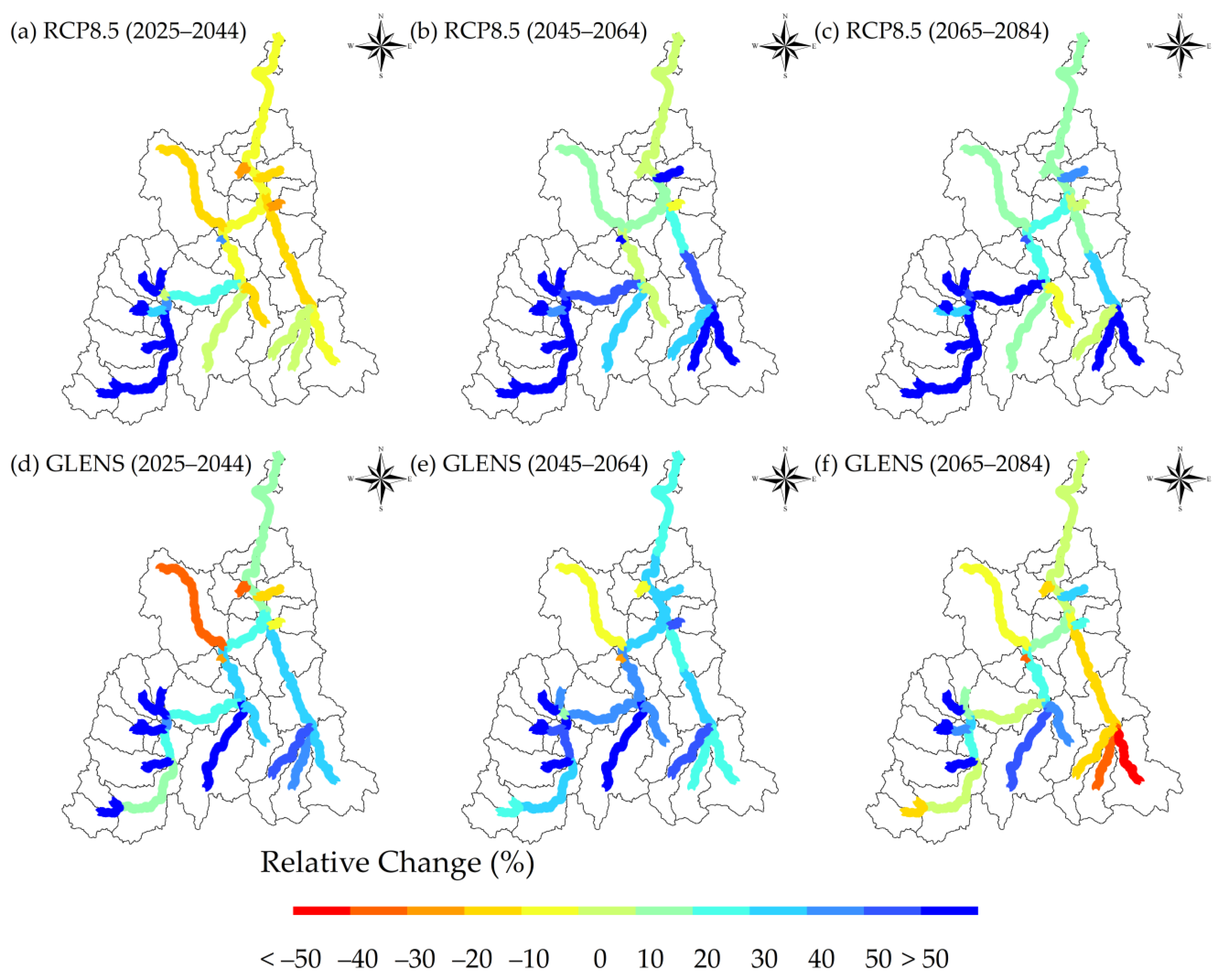
This section further explores the SRM impact on hydrological extremes of the KRB using the maximum daily flow (Figure 10) and extreme high flow Q5 (Figure 11) indices. Under RCP8.5, the maximum daily flow in the KRB increases significantly during the 2045–2064 and 2065–2084 periods across the basin, particularly in the south-western (Neggiri River) and south-eastern (Lebir River) regions. Increases of the maximum daily flows in the upstream regions would definitely affect the middle and downstream of the basin, where the major towns are located. The GLENS experiment helps to reduce the degree of change in maximum daily flow in the KRB, particularly in the Lebir River system, as shown in Figure 10f.
The absolute values and relative changes of high flow (Q5) at the Jambatan Guillermard station under GLENS and RCP8.5 are shown in Figure 11. Higher Q5 values were found during the flooding period from November to January, which thus becomes the focus of this analysis. In general, GLENS decreases the Q5 values by 24 to 33.6% in December, which is greater than the RCP8.5 experiment of 2.8 to −13.7%. In addition, in January, increases of Q5 under the RCP8.5 experiment (36.3 to 59.7%) were offset by the GLENS experiment (21.5 to 33.9%). These results are consistent with a global-scale SRM assessment conducted by Wei et al. [23], who found decreases of Q5 in Peninsular Malaysia under the G4 experiment as compared to RCP4.5 during the 2030–2069 period.
4. Discussion
In comparison to the historical period, SRM lessens the changes in peak extremes in the KRB anticipated by RCP8.5. For instance, precipitation, streamflow and high flows are projected to increase significantly under RCP8.5 during the flooding season, which would increase less or even decrease under GLENS, consistent with the findings reported by Wei et al. [23]. Jones, et al. [60] emphasized that SRM might partially offset the global warming effect and reduce the number of extreme storms. The reduction of extreme events may be explained by the Clausius-Clapeyron relation, where smaller increases in global mean temperature under SRM result in smaller increases in atmospheric water content [20]. Lower atmospheric water content causes a drop in specific humidity, which modifies how the atmosphere circulates humidity from sources to sinks.
SRM modelling commonly takes into account a single scenario, considering a scientific perspective more than policy, and sometimes includes unrealistic conditions [61]. For example, some SRM scenarios employ cooling strategies since 2020, while the others employ a substantial cooling for a bigger response [61]. Similarly, this study only considered GLENS, which employed a feedback-control strategy and injection of stratospheric aerosols at four different locations, as described in Section 2.2 [34]. This may make comparison difficult among SRM scenarios and also with non-SRM scenarios, particularly the latest Shared Socioeconomic Pathways (SSPs) under CMIP6. Hence, more climate models and SRM strategies, i.e., GeoMIP [12] and Assessing Responses and Impacts of Solar climate intervention on the Earth system (ARISE) [62], need to be considered in future studies to minimize the climate model uncertainty issue and to capture an overall picture of SRM impact at the river basin scale.
Interestingly, SRM might result in a drier condition in the dry season (February to August) in the KRB as compared to RCP8.5 in the future, as shown in Figure 5 and Figure 9. This situation may exacerbate the water supply shortage issue in the Kelantan state, which is currently influenced by not only the climatic factor but also the outmoded water piping, insufficient water treatment capacity, population growth and agricultural demand [33,63]. The variability of precipitation and temperature could significantly affect the paddy yields in the downstream part of the basin [64]. This raises the possibility of conducting more specific study of the SRM impact on water supply and agricultural sectors in tropical regions. Coupling of SWAT+ with MODFLOW should be considered to better model the flow of groundwater and its interaction with surface water [65], especially for river basins that use groundwater as their primary source of freshwater, like the KRB.
5. Conclusions
This study provides novel insight into the solar radiation management (SRM) on hydro-climatic extremes at the basin level in Southeast Asia, focusing in the Kelantan River Basin (KRB), Malaysia. The entire study framework began with the bias correction of the Stratospheric Aerosol Geoengineering Large Ensemble (GLENS) climate projections, followed by the calibration and validation of the latest Soil and Water Assessment Tool Plus (SWAT+) model. Finally, the bias-corrected GLENS projections were incorporated into the calibrated SWAT+ model to project the hydro-climatic conditions and their extreme changes for the 2025–2044, 2045–2064 and 2065–2084 periods in correspondence to the 1985–2004 baseline period.
The GLENS experiments show precipitation in the KRB will become less intense as compared to RCP8.5 at the annual scale and during the early north-east monsoon season from November to January, where massive flood events normally occur. However, the dry season from February to May will also experience comparable drops in monthly precipitation (Figure 5a). In short, decreases of monthly precipitation under SRM could be useful in reducing the flood risk but may also make the water shortage problem worse. There is a remarkable cooling of mean maximum and minimum temperatures under SRM over the KRB, but the mean minimum temperature decrease is not as significant as the mean maximum temperature. For instance, annual mean maximum and minimum temperatures are projected to increase only by 0.26 to 0.42 °C and 0.57 to 0.6 °C by the end of 21st century, compared to 1.02 to 2.88 °C and 1.32 to 3.56 °C under RCP8.5, respectively.
In term of extreme analysis, SRM could effectively reduce the number of heavy (R10 mm), very heavy (R20 mm) and violent (R50 mm) precipitation days over the KRB in the future. On the other hand, the changes of annual maximum daily rainfall amount (Rx1d) between the GLENS and RCP8.5 experiments are similar during the 2025–2044 period; SRM impact appears to be significant during the 2045–2064 and 2065–2084 periods. SRM tended to reduce the magnitude of R50 mm and Rx1d significantly for the climate stations located in the south-western and middle parts of the basin in the 2065–2084 period.
SWAT+ could adequately capture the daily and monthly streamflow variability at the Jambatan Guillermard station in the KRB, which was then used for the hydro-climatic simulations. Similar to the precipitation changes, the magnitude of increases in monthly streamflow in December and January under RCP8.5 can be effectively reduced by SRM. In addition, SRM also helps to reduce the amount of maximum daily flows mainly in the south-western (Neggiri River) and south-eastern (Lebir River) regions, as well as the high flow (Q5) at the Jambatan Guillermard station from November to January. However, a similar lesser precipitation situation is projected under the GLENS experiment during the driest months of the basin, from March to May. SRM may therefore be useful in reducing the risk of flooding, but does not address the problem of water shortage.
This study should be repeated in other tropical river basins as well as in Southeast Asia, so that a fair comparison can be made to better understand the SRM impact. In addition, additional SRM research on the water supply and agricultural sectors, i.e., oil palm and paddy, are needed in the future since different crops have different response to the changes in precipitation and temperature. Due to the disparity of SRM strategies, a further study could consider the application of different SRM climate projections and experiments, such as the GeoMIP and ARISE models. Lastly, integration of SWAT+ and MODFLOW needs to be further explored to better simulate the groundwater flows, which help in drought risk assessment.
Author Contributions
Conceptualization, M.L.T., L.J. and H.K.; methodology, M.L.T., L.J. and H.K.; software, M.L.T. and L.J.; validation, M.L.T. and L.J.; formal analysis, M.L.T. and L.J.; investigation, M.L.T., L.J. and H.K.; resources, M.L.T. and H.K.; data curation, M.L.T. and H.K.; writing—original draft preparation, M.L.T.; writing—review and editing, L.J., H.K., H.X.D. and F.Z.; project administration, H.K.; funding acquisition, M.L.T. and H.K. All authors have read and agreed to the published version of the manuscript.
Funding
The work was funded by the Degrees Modelling Fund (formerly DECIMALS), a partnership between the Degrees Initiative and The World Academy of Sciences (TWAS) under the project entitled “Investigating the Impact of Solar Geoengineering on Hydro-climatic Extreme in Southeast Asia” with the Contract No. 4500438109 and Grant Agreement (GA) project number 10-FR324031337. This research was also funded by the Ministry of Higher Education Malaysia under the long-term research grant scheme project 2, grant number LRGS/1/2020/UKM-USM/01/6/2, which is under the program LRGS/1/2020/UKM/01/6.
Data Availability Statement
The Stratospheric Aerosol Geoengineering Large Ensemble (GLENS) can be retrieved from the website: https://www.cesm.ucar.edu/projects/community-projects/GLENS/ (accessed on 15 November 2022).
Acknowledgments
The authors would like to thank the Malaysian Meteorological Department (MMD), Department of Irrigation and Drainage (DID), Department of Agricultural Malaysia (DOA), and National Geospatial Centre (PGN) for providing hydro-climatic and geospatial data for the study. HXD is supported by a grant for basic research (No. CSCB21-MTTN-07) from Nong Lam University—Ho Chi Minh City.
Conflicts of Interest
The authors declare no conflict of interest.
References
- Islam, M.B.; Huda, M.B.; Rather, N.A.; Eslamian, S. Potential of Solar Energy in India, Ch. 10 in Handbook of Eurasian Forecasting; Nova Science Publishers: New York, NY, USA, 2022. [Google Scholar]
- Gudmundsson, L.; Bremnes, J.B.; Haugen, J.E.; Engen-Skaugen, T. Technical Note: Downscaling RCM precipitation to the station scale using statistical transformations—A comparison of methods. Hydrol. Earth Syst. Sci. 2012, 16, 3383–3390. [Google Scholar] [CrossRef] [Green Version]
- Ridder, N.N.; Ukkola, A.M.; Pitman, A.J.; Perkins-Kirkpatrick, S.E. Increased occurrence of high impact compound events under climate change. Npj Clim. Atmos. Sci. 2022, 5, 3. [Google Scholar] [CrossRef]
- Ward, P.J.; Blauhut, V.; Bloemendaal, N.; Daniell, J.E.; de Ruiter, M.C.; Duncan, M.J.; Emberson, R.; Jenkins, S.F.; Kirschbaum, D.; Kunz, M.; et al. Review article: Natural hazard risk assessments at the global scale. Nat. Hazards Earth Syst. Sci. 2020, 20, 1069–1096. [Google Scholar] [CrossRef] [Green Version]
- Fowler, H.J.; Lenderink, G.; Prein, A.F.; Westra, S.; Allan, R.P.; Ban, N.; Barbero, R.; Berg, P.; Blenkinsop, S.; Do, H.X.; et al. Anthropogenic intensification of short-duration rainfall extremes. Nat. Rev. Earth Environ. 2021, 2, 107–122. [Google Scholar] [CrossRef]
- Eccles, R.; Zhang, H.; Hamilton, D. A review of the effects of climate change on riverine flooding in subtropical and tropical regions. J. Water Clim. Chang. 2019, 10, 687–707. [Google Scholar] [CrossRef] [Green Version]
- IPCC. Summary for Policymakers. Climate Change 2021: The Physical Science Basis. In Contribution of Working Group I to the Sixth Assessment Report of the Intergovernmental Panel on Climate Change; Masson-Delmotte, V., Zhai, P., Pirani, A., Connors, S.L., Péan, C., Berger, S., Caud, N., Chen, Y., Goldfarb, L., Gomis, M.I., et al., Eds.; Cambridge University Press: Cambridge, UK; New York, NY, USA, 2021. [Google Scholar]
- Kundzewicz, Z.W.; Kanae, S.; Seneviratne, S.I.; Handmer, J.; Nicholls, N.; Peduzzi, P.; Mechler, R.; Bouwer, L.M.; Arnell, N.; Mach, K.; et al. Flood risk and climate change: Global and regional perspectives. Hydrol. Sci. J. 2014, 59, 1–28. [Google Scholar] [CrossRef] [Green Version]
- Jongman, B. Effective adaptation to rising flood risk. Nat. Commun. 2018, 9, 1986. [Google Scholar] [CrossRef] [Green Version]
- IPCC. Climate Change 2022: Impacts, Adaptation, and Vulnerability. In Contribution of Working Group II to the Sixth Assessment Report of the Intergovernmental Panel on Climate Change; Pörtner, H.-O., Roberts, D.C., Tignor, M., Poloczanska, E.S., Mintenbeck, K., Alegría, A., Craig, M., Langsdorf, S., Löschke, S., Möller, V., et al., Eds.; Cambridge University Press: Cambridge, UK; New York, NY, USA, 2022; p. 3056. [Google Scholar] [CrossRef]
- IPCC. Global Warming of 1.5°C. IPCC Spec. Rep. Impacts Glob. Warm. 2018, 1, 43–50. [Google Scholar]
- Kravitz, B.; Robock, A.; Forster, P.M.; Haywood, J.M.; Lawrence, M.G.; Schmidt, H. An overview of the Geoengineering Model Intercomparison Project (GeoMIP). J. Geophys. Res. Atmos. 2013, 118, 13103–13107. [Google Scholar] [CrossRef]
- Vaughan, N.E.; Lenton, T.M. A review of climate geoengineering proposals. Clim. Chang. 2011, 109, 745–790. [Google Scholar] [CrossRef]
- Lenton, T.M.; Vaughan, N.E. The radiative forcing potential of different climate geoengineering options. Atmos. Chem. Phys. 2009, 9, 5539–5561. [Google Scholar] [CrossRef] [Green Version]
- Kravitz, B.; MacMartin, D.G. Uncertainty and the basis for confidence in solar geoengineering research. Nat. Rev. Earth Environ. 2020, 1, 64–75. [Google Scholar] [CrossRef] [Green Version]
- Raimi, K.T. Public perceptions of geoengineering. Curr. Opin. Psychol. 2021, 42, 66–70. [Google Scholar] [CrossRef]
- Wiertz, T. Visions of Climate Control:Solar Radiation Management in Climate Simulations. Sci. Technol. Hum. Values 2016, 41, 438–460. [Google Scholar] [CrossRef]
- Tilmes, S.; Fasullo, J.; Lamarque, J.F.; Marsh, D.R.; Mills, M.; Alterskjaer, K.; Muri, H.; Kristjansson, J.E.; Boucher, O.; Schulz, M.; et al. The hydrological impact of geoengineering in the Geoengineering Model Intercomparison Project (GeoMIP). J. Geophys. Res. Atmos. 2013, 118, 11036–11058. [Google Scholar] [CrossRef] [Green Version]
- Dagon, K.; Schrag, D.P. Exploring the Effects of Solar Radiation Management on Water Cycling in a Coupled Land–Atmosphere Model. J. Clim. 2016, 29, 2635–2650. [Google Scholar] [CrossRef]
- Pinto, I.; Jack, C.; Lennard, C.; Tilmes, S.; Odoulami, R.C. Africa’s Climate Response to Solar Radiation Management With Stratospheric Aerosol. Geophys. Res. Lett. 2020, 47, e2019GL086047. [Google Scholar] [CrossRef] [Green Version]
- Kuswanto, H.; Kravitz, B.; Miftahurrohmah, B.; Fauzi, F.; Sopahaluwaken, A.; Moore, J. Impact of solar geoengineering on temperatures over the Indonesian Maritime Continent. Int. J. Climatol. 2022, 42, 2795–2814. [Google Scholar] [CrossRef]
- Russell, L.M.; Rasch, P.J.; Mace, G.M.; Jackson, R.B.; Shepherd, J.; Liss, P.; Leinen, M.; Schimel, D.; Vaughan, N.E.; Janetos, A.C.; et al. Ecosystem impacts of geoengineering: A review for developing a science plan. Ambio 2012, 41, 350–369. [Google Scholar] [CrossRef] [Green Version]
- Wei, L.R.; Ji, D.Y.; Miao, C.Y.; Muri, H.; Moore, J.C. Global streamflow and flood response to stratospheric aerosol geoengineering. Atmos. Chem. Phys. 2018, 18, 16033–16050. [Google Scholar] [CrossRef] [Green Version]
- Kleidon, A.; Kravitz, B.; Renner, M. The hydrological sensitivity to global warming and solar geoengineering derived from thermodynamic constraints. Geophys. Res. Lett. 2015, 42, 138–144. [Google Scholar] [CrossRef]
- Camilloni, I.; Montroull, N.; Gulizia, C.; Saurral, R.I. La Plata Basin Hydroclimate Response to Solar Radiation Modification With Stratospheric Aerosol Injection. Front. Clim. 2022, 4, 763983. [Google Scholar] [CrossRef]
- Cheng, W.; MacMartin, D.; Dagon, K.; Kravitz, B.; Tilmes, S.; Richter, J.H.; Mills, M.J.; Simpson, I.R. Soil Moisture and Other Hydrological Changes in a Stratospheric Aerosol Geoengineering Large Ensemble. J. Geophys. Res. Atmos. 2019, 124, 12773–12793. [Google Scholar] [CrossRef]
- Tew, Y.L.; Tan, M.L.; Juneng, L.; Chun, K.P.; Hassan, M.H.b.; Osman, S.b.; Samat, N.; Chang, C.K.; Kabir, M.H. Rapid Extreme Tropical Precipitation and Flood Inundation Mapping Framework (RETRACE): Initial Testing for the 2021–2022 Malaysia Flood. ISPRS Int. J. Geo-Inf. 2022, 11, 378. [Google Scholar] [CrossRef]
- Anua, N.; Tan, M.L.; Chan, N.W. Community resilience to the 2014 flood: A case study in the Kampung Manek Urai Lama, Kuala Krai, Kelantan. GEOGRAFIA—Malays. J. Soc. Space 2021, 17, 196–210. [Google Scholar] [CrossRef]
- Tan, M.L.; Ibrahim, A.L.; Yusop, Z.; Chua, V.P.; Chan, N.W. Climate change impacts under CMIP5 RCP scenarios on water resources of the Kelantan River Basin, Malaysia. Atmos. Res. 2017, 189, 1–10. [Google Scholar] [CrossRef]
- Tan, M.L.; Liang, J.; Samat, N.; Chan, N.W.; Haywood, J.M.; Hodges, K. Hydrological Extremes and Responses to Climate Change in the Kelantan River Basin, Malaysia, Based on the CMIP6 HighResMIP Experiments. Water 2021, 13, 1472. [Google Scholar] [CrossRef]
- Tan, M.L.; Ibrahim, A.L.; Cracknell, A.P.; Yusop, Z. Changes in precipitation extremes over the Kelantan River Basin, Malaysia. Int. J. Climatol. 2017, 37, 3780–3797. [Google Scholar] [CrossRef]
- Tan, M.L.; Gassman, P.W.; Srinivasan, R.; Arnold, J.G.; Yang, X. A Review of SWAT Studies in Southeast Asia: Applications, Challenges and Future Directions. Water 2019, 11, 914. [Google Scholar] [CrossRef] [Green Version]
- Tan, M.L.; Juneng, L.; Tangang, F.T.; Samat, N.; Chan, N.W.; Yusop, Z.; Ngai, S.T. SouthEast Asia HydrO-meteorological droughT (SEA-HOT) framework: A case study in the Kelantan River Basin, Malaysia. Atmos. Res. 2020, 246, 105155. [Google Scholar] [CrossRef]
- Mills, M.J.; Richter, J.H.; Tilmes, S.; Kravitz, B.; MacMartin, D.G.; Glanville, A.A.; Tribbia, J.J.; Lamarque, J.-F.; Vitt, F.; Schmidt, A.; et al. Radiative and Chemical Response to Interactive Stratospheric Sulfate Aerosols in Fully Coupled CESM1(WACCM). J. Geophys. Res. Atmos. 2017, 122, 13–061. [Google Scholar] [CrossRef]
- MacMartin, D.G.; Kravitz, B.; Tilmes, S.; Richter, J.H.; Mills, M.J.; Lamarque, J.-F.; Tribbia, J.J.; Vitt, F. The Climate Response to Stratospheric Aerosol Geoengineering Can Be Tailored Using Multiple Injection Locations. J. Geophys. Res. Atmos. 2017, 122, 12–574. [Google Scholar] [CrossRef]
- Tilmes, S.; Richter, J.H.; Kravitz, B.; MacMartin, D.G.; Mills, M.J.; Simpson, I.R.; Glanville, A.S.; Fasullo, J.T.; Phillips, A.S.; Lamarque, J.-F.; et al. CESM1(WACCM) Stratospheric Aerosol Geoengineering Large Ensemble Project. Bull. Am. Meteorol. Soc. 2018, 99, 2361–2371. [Google Scholar] [CrossRef]
- Bieger, K.; Arnold, J.G.; Rathjens, H.; White, M.J.; Bosch, D.D.; Allen, P.M.; Volk, M.; Srinivasan, R. Introduction to SWAT+, A Completely Restructured Version of the Soil and Water Assessment Tool. JAWRA J. Am. Water Resour. Assoc. 2017, 53, 115–130. [Google Scholar] [CrossRef]
- Arnold, J.G.; Bieger, K.; White, M.J.; Srinivasan, R.; Dunbar, J.A.; Allen, P.M. Use of Decision Tables to Simulate Management in SWAT+. Water 2018, 10, 713. [Google Scholar] [CrossRef] [Green Version]
- Neitsch, S.L.; Arnold, J.G.; Kiniry, J.R.; Grassland, J.R.W. Soil and Water Assessment Tool Theoretical Documentation Version 2009; Agricultural Research Service Blackland Research Center: Temple, TX, USA, 2011.
- Singh, L.; Saravanan, S. Simulation of monthly streamflow using the SWAT model of the Ib River watershed, India. HydroResearch 2020, 3, 95–105. [Google Scholar] [CrossRef]
- Maraun, D. Bias Correcting Climate Change Simulations—A Critical Review. Curr. Clim. Chang. Rep. 2016, 2, 211–220. [Google Scholar] [CrossRef] [Green Version]
- Mendez, M.; Maathuis, B.; Hein-Griggs, D.; Alvarado-Gamboa, L.-F. Performance Evaluation of Bias Correction Methods for Climate Change Monthly Precipitation Projections over Costa Rica. Water 2020, 12, 482. [Google Scholar] [CrossRef] [Green Version]
- Boé, J.; Terray, L.; Habets, F.; Martin, E. Statistical and dynamical downscaling of the Seine basin climate for hydro-meteorological studies. Int. J. Climatol. 2007, 27, 1643–1655. [Google Scholar] [CrossRef]
- Patel, J.; Gnanaseelan, C.; Chowdary, J.S.; Parekh, A. A quantile mapping approach-based bias correction in Coupled Model Intercomparison Project Phase 5 models for decadal temperature predictions over India. Int. J. Climatol. 2022, 42, 2455–2469. [Google Scholar] [CrossRef]
- Tan, M.L.; Juneng, L.; Tangang, F.T.; Chan, N.W.; Ngai, S.T. Future hydro-meteorological drought of the Johor River Basin, Malaysia, based on CORDEX-SEA projections. Hydrol. Sci. J. 2019, 64, 921–933. [Google Scholar] [CrossRef]
- Ngai, S.T.; Tangang, F.; Juneng, L. Bias correction of global and regional simulated daily precipitation and surface mean temperature over Southeast Asia using quantile mapping method. Glob. Planet. Chang. 2017, 149, 79–90. [Google Scholar] [CrossRef] [Green Version]
- Senent-Aparicio, J.; George, C.; Srinivasan, R. Introducing a new post-processing tool for the SWAT+ model to evaluate environmental flows. Environ. Model. Softw. 2021, 136, 104944. [Google Scholar] [CrossRef]
- Moriasi, D.N.; Arnold, J.G.; Van Liew, M.W.; Bingner, R.L.; Harmel, R.D.; Veith, T.L. Model Evaluation Guidelines for Systematic Quantification of Accuracy in Watershed Simulations. Trans. ASABE 2007, 50, 885–900. [Google Scholar] [CrossRef]
- Moriasi, D.N.; Gitau, M.W.; Pai, N.; Daggupati, P. Hydrologic and water quality models: Performance measures and evaluation criteria. Trans. ASABE 2015, 58, 1763–1785. [Google Scholar] [CrossRef] [Green Version]
- Data, C. Guidelines on analysis of extremes in a changing climate in support of informed decisions for adaptation. In World Meteorological Organization TD-1500; World Meteorological Organisation: Geneva, Switzerland, 2009; p. 52. [Google Scholar]
- Rupp, D.E.; Abatzoglou, J.T.; Hegewisch, K.C.; Mote, P.W. Evaluation of CMIP5 20th century climate simulations for the Pacific Northwest USA. J. Geophys. Res. Atmos. 2013, 118, 10884–10906. [Google Scholar] [CrossRef]
- Stjern, C.W.; Samset, B.H.; Boucher, O.; Iversen, T.; Lamarque, J.F.; Myhre, G.; Shindell, D.; Takemura, T. How aerosols and greenhouse gases influence the diurnal temperature range. Atmos. Chem. Phys. 2020, 20, 13467–13480. [Google Scholar] [CrossRef]
- Liu, Z.; Lang, X.; Jiang, D. Impact of stratospheric aerosol intervention geoengineering on surface air temperature in China: A surface energy budget perspective. Atmos. Chem. Phys. 2022, 22, 7667–7680. [Google Scholar] [CrossRef]
- Russotto, R.D.; Ackerman, T.P. Changes in clouds and thermodynamics under solar geoengineering and implications for required solar reduction. Atmos. Chem. Phys. 2018, 18, 11905–11925. [Google Scholar] [CrossRef] [Green Version]
- Jiménez-Navarro, I.C.; Jimeno-Sáez, P.; López-Ballesteros, A.; Pérez-Sánchez, J.; Senent-Aparicio, J. Impact of Climate Change on the Hydrology of the Forested Watershed That Drains to Lake Erken in Sweden: An Analysis Using SWAT+ and CMIP6 Scenarios. Forests 2021, 12, 1803. [Google Scholar] [CrossRef]
- Mendonça dos Santos, F.; Proença de Oliveira, R.; Augusto Di Lollo, J. Effects of Land Use Changes on Streamflow and Sediment Yield in Atibaia River Basin—SP, Brazil. Water 2020, 12, 1711. [Google Scholar] [CrossRef]
- Beven, K.; Binley, A. The future of distributed models: Model calibration and uncertainty prediction. Hydrol. Process. 1992, 6, 279–298. [Google Scholar] [CrossRef]
- Pereira, D.D.; Martinez, M.A.; Pruski, F.F.; da Silva, D.D. Hydrological simulation in a basin of typical tropical climate and soil using the SWAT model part I: Calibration and validation tests. J. Hydrol. Reg. Stud. 2016, 7, 14–37. [Google Scholar] [CrossRef] [Green Version]
- Leta, O.T.; El-Kadi, A.I.; Dulai, H.; Ghazal, K.A. Assessment of climate change impacts on water balance components of Heeia watershed in Hawaii. J. Hydrol. Reg. Stud. 2016, 8, 182–197. [Google Scholar] [CrossRef] [Green Version]
- Jones, A.C.; Hawcroft, M.K.; Haywood, J.M.; Jones, A.; Guo, X.; Moore, J.C. Regional Climate Impacts of Stabilizing Global Warming at 1.5 K Using Solar Geoengineering. Earth’s Future 2018, 6, 230–251. [Google Scholar] [CrossRef] [Green Version]
- MacMartin, D.G.; Visioni, D.; Kravitz, B.; Richter, J.H.; Felgenhauer, T.; Lee, W.R.; Morrow, D.R.; Parson, E.A.; Sugiyama, M. Scenarios for modeling solar radiation modification. Proc. Natl. Acad. Sci. USA 2022, 119, e2202230119. [Google Scholar] [CrossRef]
- Richter, J.H.; Visioni, D.; MacMartin, D.G.; Bailey, D.A.; Rosenbloom, N.; Dobbins, B.; Lee, W.R.; Tye, M.; Lamarque, J.F. Assessing Responses and Impacts of Solar climate intervention on the Earth system with stratospheric aerosol injection (ARISE-SAI): Protocol and initial results from the first simulations. Geosci. Model Dev. 2022, 15, 8221–8243. [Google Scholar] [CrossRef]
- Abdul Ghani, L.; Ali, N.a.; Nazaran, I.S.; Hanafiah, M.M. Environmental Performance of Small-Scale Seawater Reverse Osmosis Plant for Rural Area Water Supply. Membranes 2021, 11, 40. [Google Scholar] [CrossRef]
- Firdaus, R.B.R.; Mou Leong, T.; Rahmat, S.R.; Senevi Gunaratne, M. Paddy, rice and food security in Malaysia: A review of climate change impacts. Cogent Soc. Sci. 2020, 6, 1818373. [Google Scholar] [CrossRef]
- Bailey, R.T.; Park, S.; Bieger, K.; Arnold, J.G.; Allen, P.M. Enhancing SWAT+ simulation of groundwater flow and groundwater-surface water interactions using MODFLOW routines. Environ. Model. Softw. 2020, 126, 104660. [Google Scholar] [CrossRef]
Figure 1.
(a) Kelantan River Basin and its location within the (b) Malaysian and (c) Southeast Asian regions.
Figure 1.
(a) Kelantan River Basin and its location within the (b) Malaysian and (c) Southeast Asian regions.

Figure 2.
The conceptual framework of SRM hydro-climatic impact assessment using SWAT+.

Figure 3.
The comparison of catchment average daily rainfall, maximum temperature and minimum temperature climatology of the raw GCM simulation and bias-corrected GCM simulation against the observed values from 1981–2009.
Figure 3.
The comparison of catchment average daily rainfall, maximum temperature and minimum temperature climatology of the raw GCM simulation and bias-corrected GCM simulation against the observed values from 1981–2009.

Figure 4.
The comparison of catchment averaged daily rainfall and maximum temperature and minimum temperature climatology of the raw GCM simulation and bias-corrected GCM simulation against the observed values from 1981–2009.
Figure 4.
The comparison of catchment averaged daily rainfall and maximum temperature and minimum temperature climatology of the raw GCM simulation and bias-corrected GCM simulation against the observed values from 1981–2009.

Figure 5.
Comparison of climatology and relative changes of monthly (a,d) precipitation, (b,e) mean maximum temperature and (c,f) mean minimum temperature of the Kelantan River Basin between the historical (1985–2004) and future periods (2025–2044, 2045–2064 and 2065–2084) under the RCP8.5 and GLENS scenarios.

Figure 6.
Relative changes in the R10 mm, R20 mm, R50 mm and Rx1d indices under the RCP8.5 and GLENS simulations across the stations during the 2025–2044, 2045–2064 and 2065–2084 periods.
Figure 6.
Relative changes in the R10 mm, R20 mm, R50 mm and Rx1d indices under the RCP8.5 and GLENS simulations across the stations during the 2025–2044, 2045–2064 and 2065–2084 periods.

Figure 7.
Boxplots of the (a) R10 mm, (b) R20 mm, (c) R50 mm and (d) Rx1d values at the evaluated climate stations during the 2025–2044, 2045–2064 and 2065–2084 periods.
Figure 7.
Boxplots of the (a) R10 mm, (b) R20 mm, (c) R50 mm and (d) Rx1d values at the evaluated climate stations during the 2025–2044, 2045–2064 and 2065–2084 periods.

Figure 8.
Observed and simulated flows at the Jambatan Guillermard in the Kelantan River Basin for both (a) monthly and (b) daily timescales.
Figure 8.
Observed and simulated flows at the Jambatan Guillermard in the Kelantan River Basin for both (a) monthly and (b) daily timescales.

Figure 9.
Climatology (a) and relative changes (b) of the streamflow at the Jambatan Guillermard between the historical (1985–2004) and future periods (2025–2044, 2045–2064 and 2065–2084) under RCP8.5 and GLENS.
Figure 9.
Climatology (a) and relative changes (b) of the streamflow at the Jambatan Guillermard between the historical (1985–2004) and future periods (2025–2044, 2045–2064 and 2065–2084) under RCP8.5 and GLENS.

Figure 10.
Relative changes of maximum daily flow at the sub-basin level in the KRB for GLENS and RCP8.5 during the 2025–2044, 2045–2064 and 2065–2084 periods as compared to the 1985–2004 baseline period.
Figure 10.
Relative changes of maximum daily flow at the sub-basin level in the KRB for GLENS and RCP8.5 during the 2025–2044, 2045–2064 and 2065–2084 periods as compared to the 1985–2004 baseline period.

Figure 11.
High flow (Q5) at the Jambatan Guillermard station under (a) RCP8.5 and (b) GLENS and (c) the relative changes of the 2025–2044, 2045–2064 and 2065–2084 periods from the 1985–2004 baseline period.
Figure 11.
High flow (Q5) at the Jambatan Guillermard station under (a) RCP8.5 and (b) GLENS and (c) the relative changes of the 2025–2044, 2045–2064 and 2065–2084 periods from the 1985–2004 baseline period.


Table 1.
The mean absolute error comparing the observation data and raw GLENS simulation and bias-corrected GLENS simulation.
Table 1.
The mean absolute error comparing the observation data and raw GLENS simulation and bias-corrected GLENS simulation.
| Precipitation (mm/day) | Maximum Temperature (°C) | Minimum Temperature (°C) | |
|---|---|---|---|
| GLENS (raw) | 0.97 | 2.1 | 3.3 |
| GLENS (bias-corrected) | 0.21 | 0.27 | 0.3 |
Table 2.
SWAT+ calibration parameter sensitivity, description, range and adjusted value.
| Rank | Parameter | Unit | Description | Type | Range | Adjusted |
|---|---|---|---|---|---|---|
| 1 | CANMX | Mm/H20 | Maximum canopy storage | 1 absval | 0–100 | 80 |
| 2 | ESCO | - | Soil evaporation compensation coefficient | 1 absval | 0–1 | 0.8 |
| 3 | LATQ_CO | - | Lateral flow coefficient | 1 absval | 0–1 | 0.98 |
| 4 | CN2 | - | Curve number condition II | 2 pctchg | −20–20 | −20 |
| 5 | SLOPE | m/m | Average slope steepness in HRU | 1 absval | 0–0.9 | 0.75 |
| 6 | SURLAG | days | Surface runoff lag coefficient | 1 absval | 1–24 | 2 |
| 7 | REVAP_MIN | m | Threshold depth of water in the shallow aquifer needed for re-evaporation or percolation to the deep aquifer to occur | 1 absval | 0–50 | 15 |
| 8 | FLO_MIN | m | Minimum aquifer storage to allow return flow | 1 absval | 0–50 | 37 |
| 9 | REVAP_CO | - | Groundwater re-evaporation coefficient | 1 absval | 0.02–0.2 | 0.1 |
| 10 | AWC | mm_H20/mm | Soil layer’s available water capacity | 2 pctchg | −20–20 | 13.73 |
| 11 | PERCO | fraction | Percolation coefficient | 1 absval | 0–1 | 0.99 |
1 Absval indicates replacement value, while 2 pctchg indicates percent change. The most sensitive parameter is ranked 1, and the least sensitive parameter is ranked 14.
Disclaimer/Publisher’s Note: The statements, opinions and data contained in all publications are solely those of the individual author(s) and contributor(s) and not of MDPI and/or the editor(s). MDPI and/or the editor(s) disclaim responsibility for any injury to people or property resulting from any ideas, methods, instructions or products referred to in the content. |
© 2023 by the authors. Licensee MDPI, Basel, Switzerland. This article is an open access article distributed under the terms and conditions of the Creative Commons Attribution (CC BY) license (https://creativecommons.org/licenses/by/4.0/).
Share and Cite
MDPI and ACS Style
Tan, M.L.; Juneng, L.; Kuswanto, H.; Do, H.X.; Zhang, F. Impacts of Solar Radiation Management on Hydro-Climatic Extremes in Southeast Asia. Water 2023, 15, 1089. https://doi.org/10.3390/w15061089
AMA Style
Tan ML, Juneng L, Kuswanto H, Do HX, Zhang F. Impacts of Solar Radiation Management on Hydro-Climatic Extremes in Southeast Asia. Water. 2023; 15(6):1089. https://doi.org/10.3390/w15061089
Chicago/Turabian StyleTan, Mou Leong, Liew Juneng, Heri Kuswanto, Hong Xuan Do, and Fei Zhang. 2023. "Impacts of Solar Radiation Management on Hydro-Climatic Extremes in Southeast Asia" Water 15, no. 6: 1089. https://doi.org/10.3390/w15061089
Note that from the first issue of 2016, this journal uses article numbers instead of page numbers. See further details here.