
An Assessment of Geospatial Analysis Combined with AHP Techniques to Identify Groundwater Potential Zones in the Pudukkottai District, Tamil Nadu, India

 , , , ,
  , , ,
, , ,  ,
,  and
and
Abstract
:1. Introduction
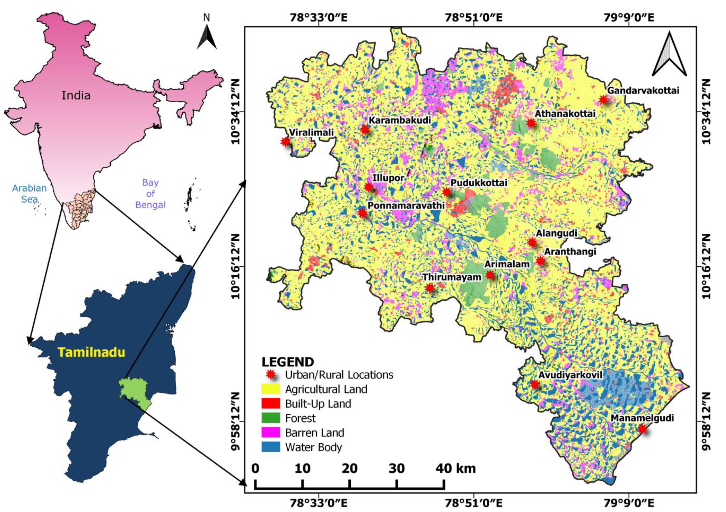
2. Study Area
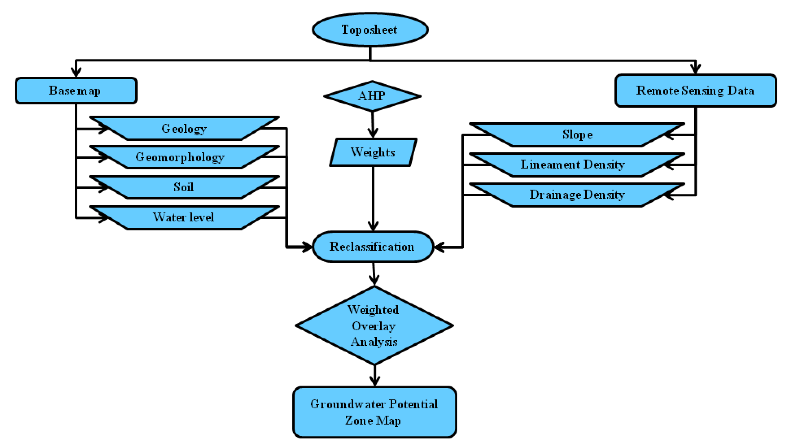
3. Materials and Methods
3.1. Weighted Overlay Analysis
3.2. Sensitivity Analysis
4. Discussion
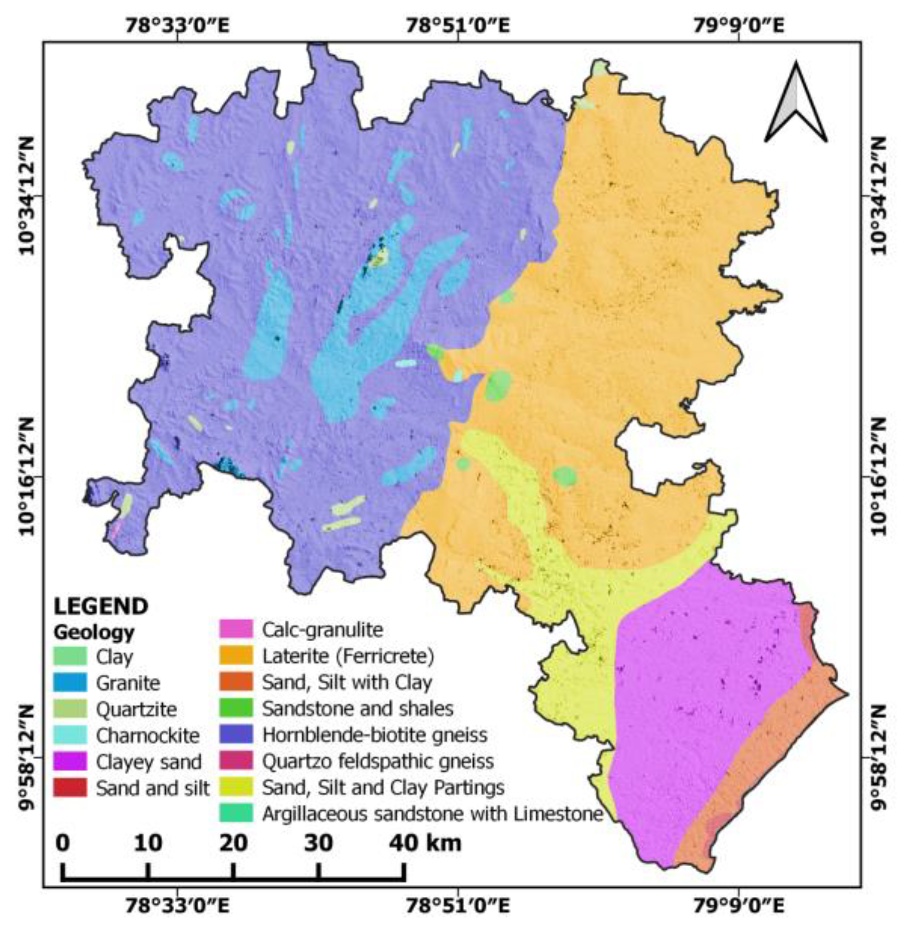
4.1. Geology
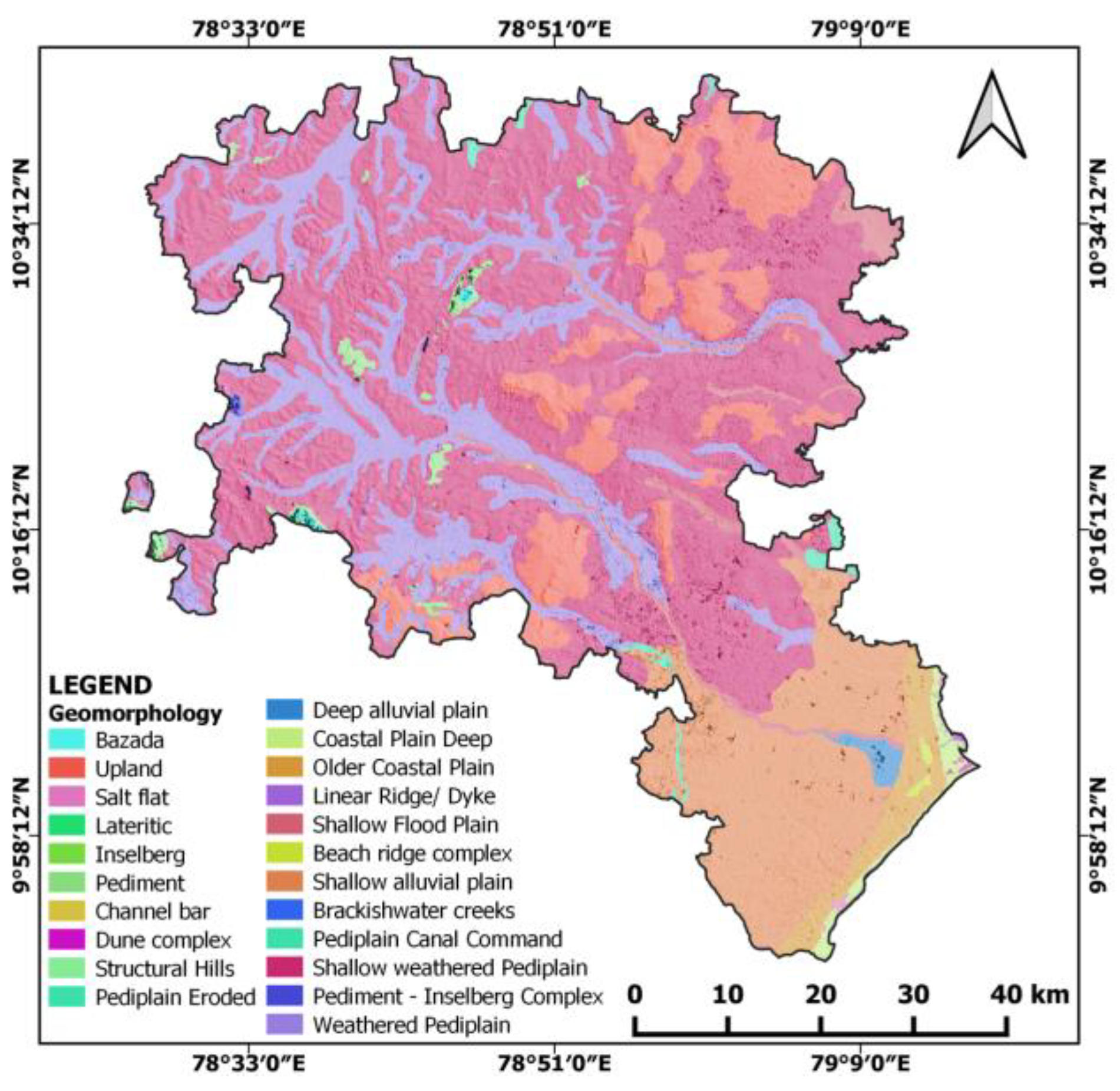
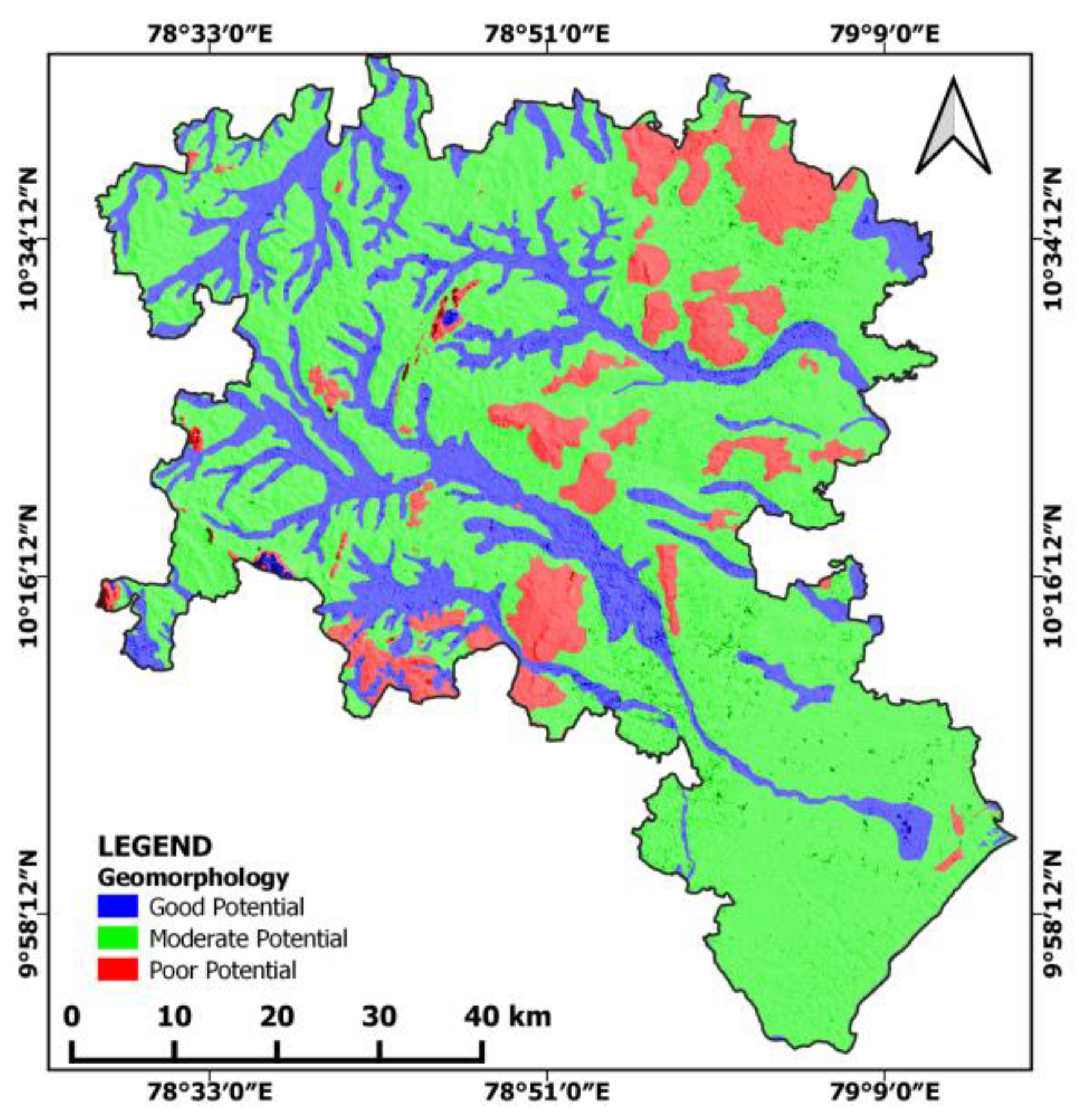
4.2. Geomorphology
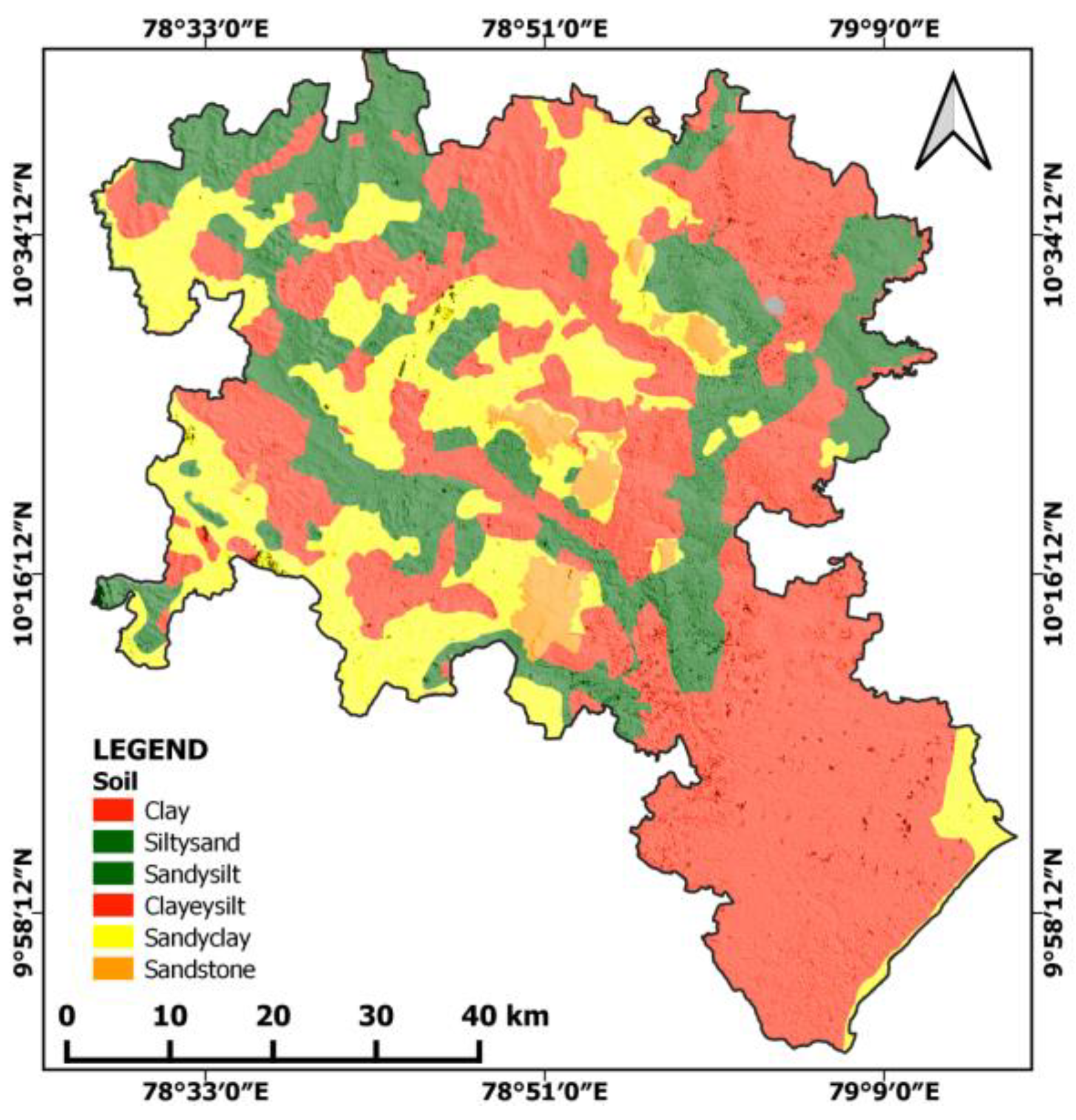
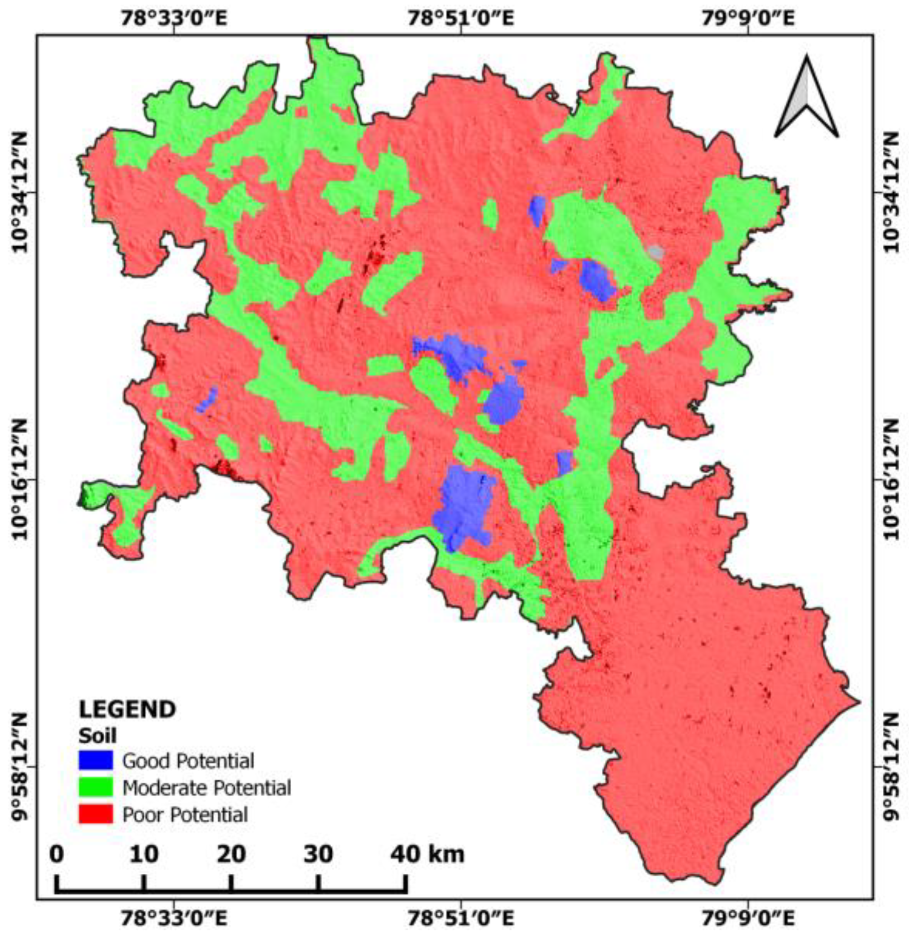
4.3. Soil
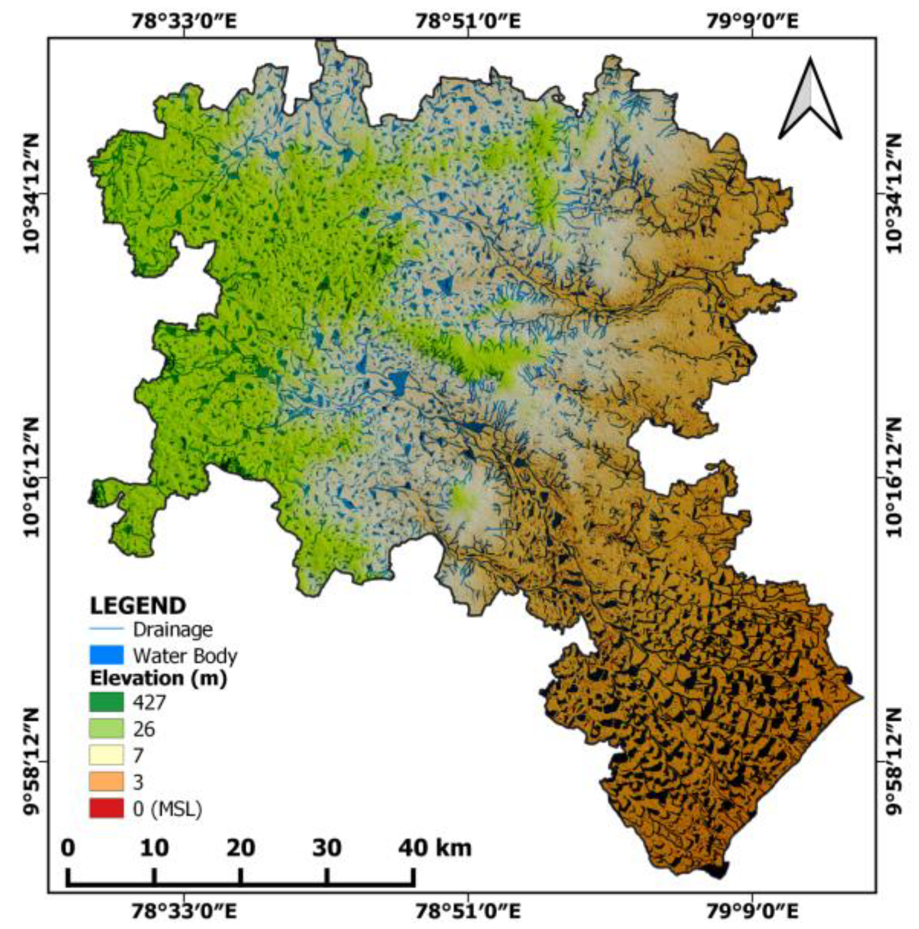
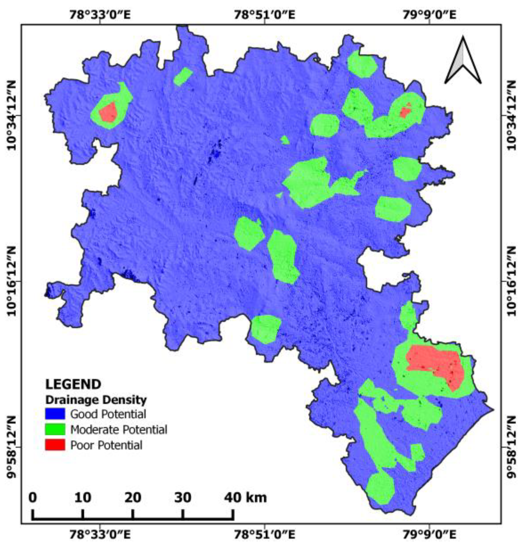
4.4. Drainage and Drainage Density
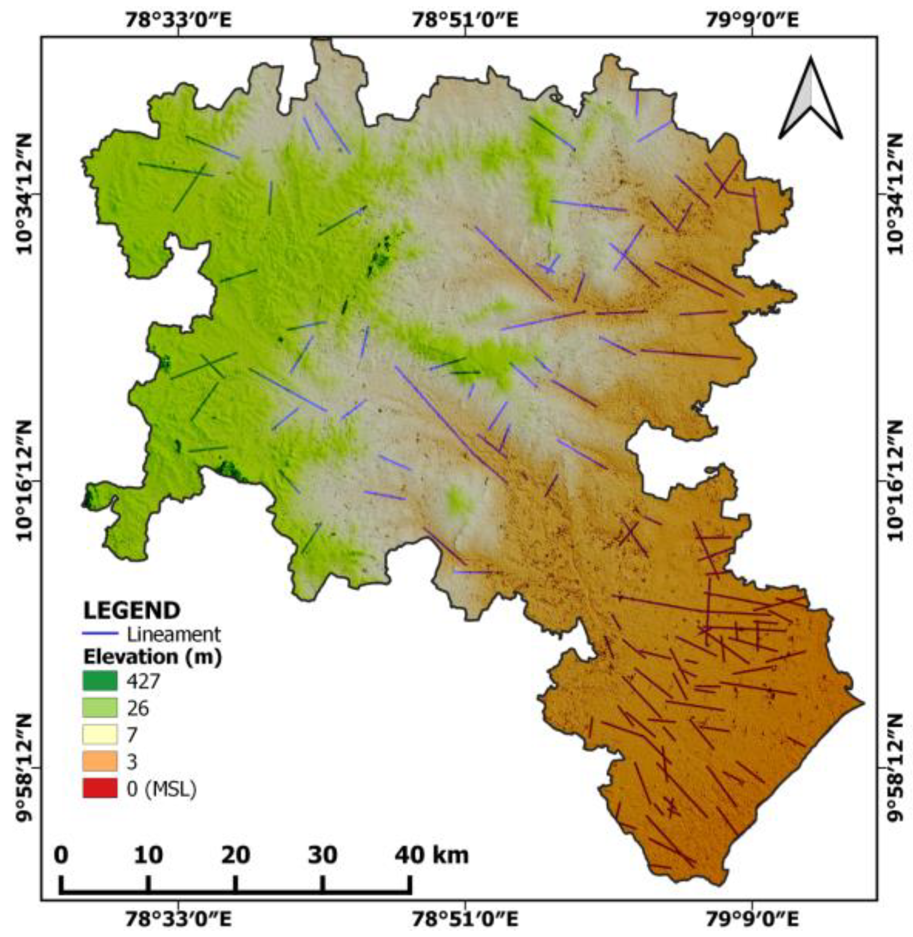
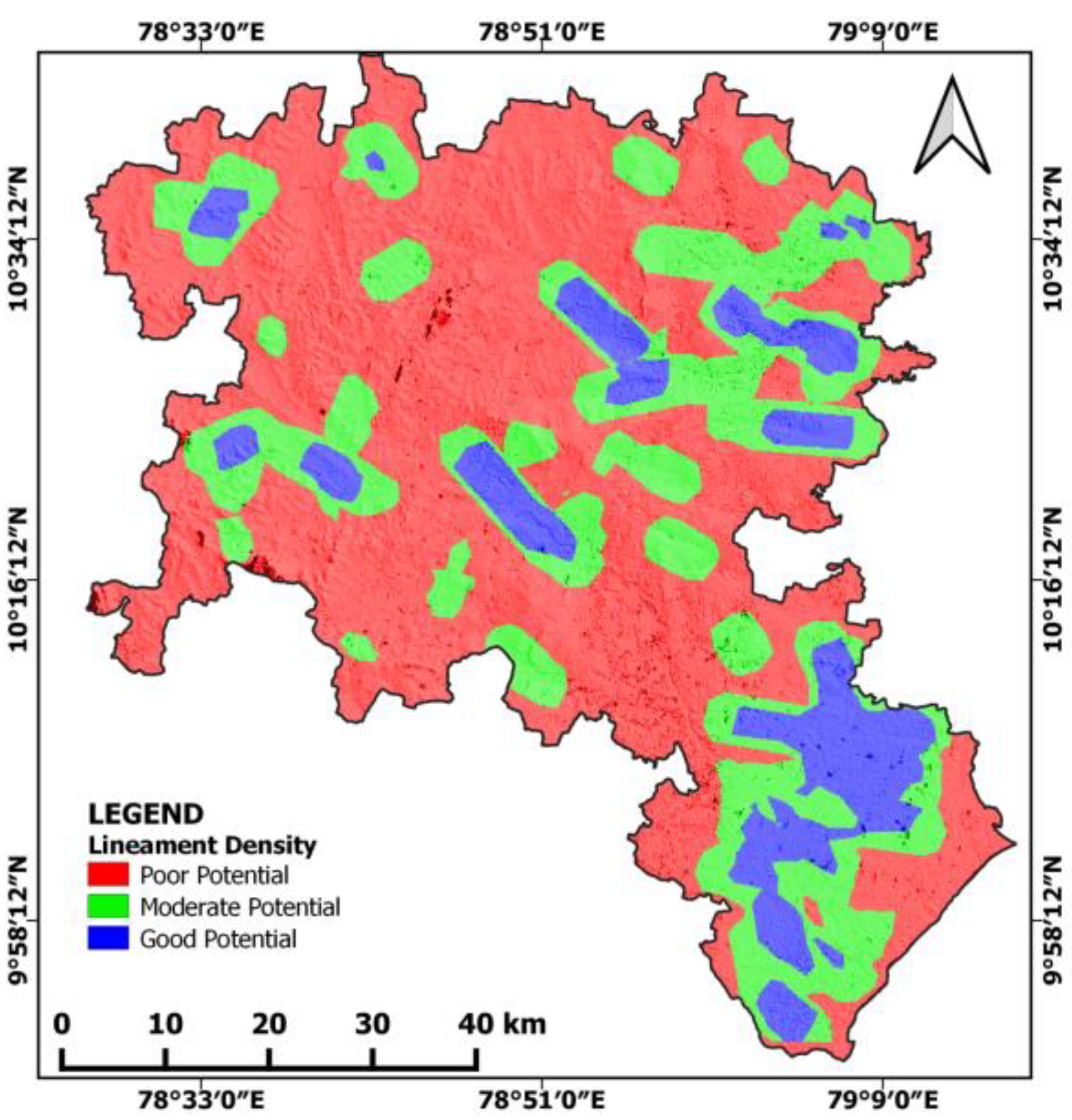
4.5. Lineament (L) and Lineament Density (LD)
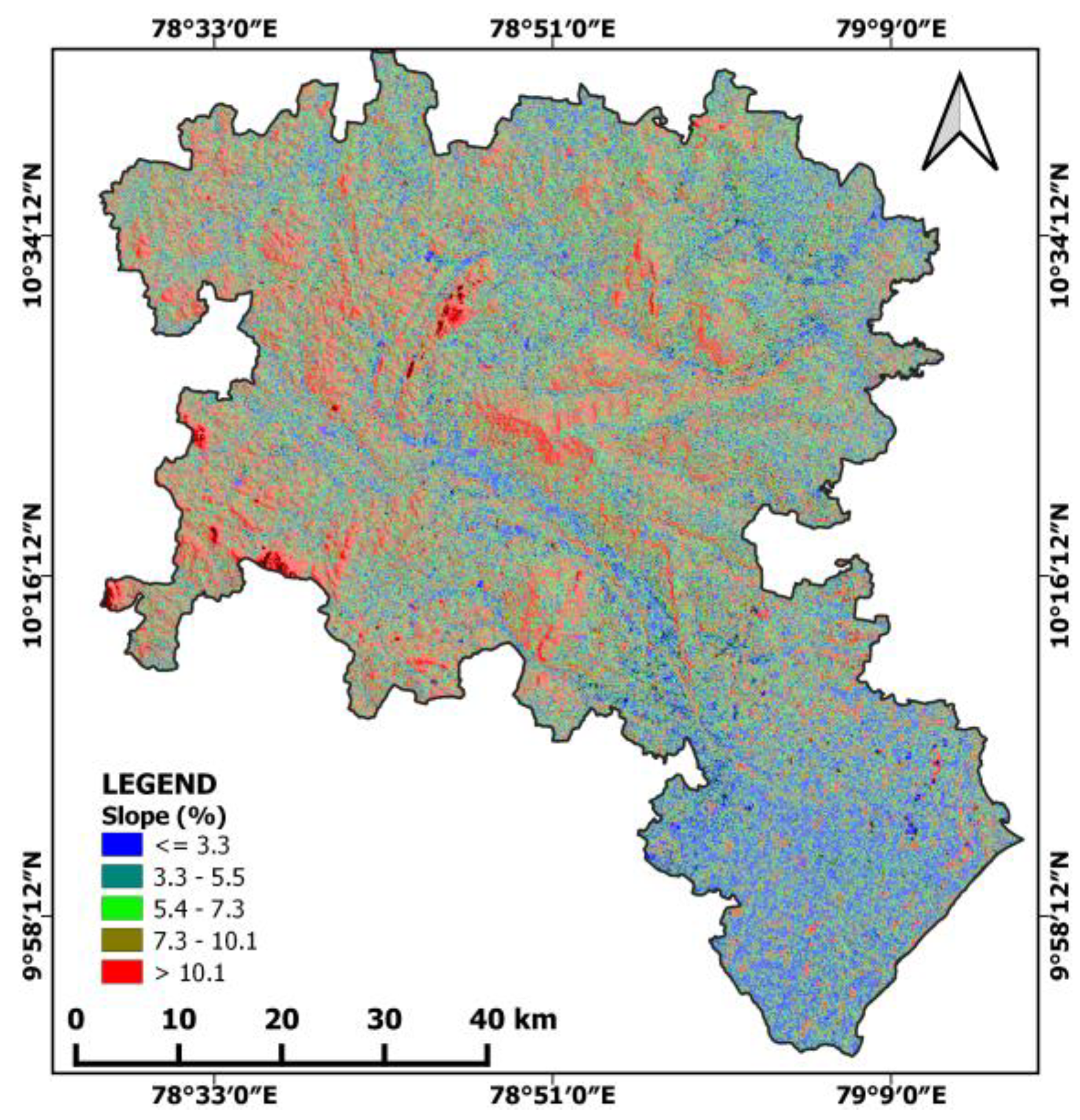
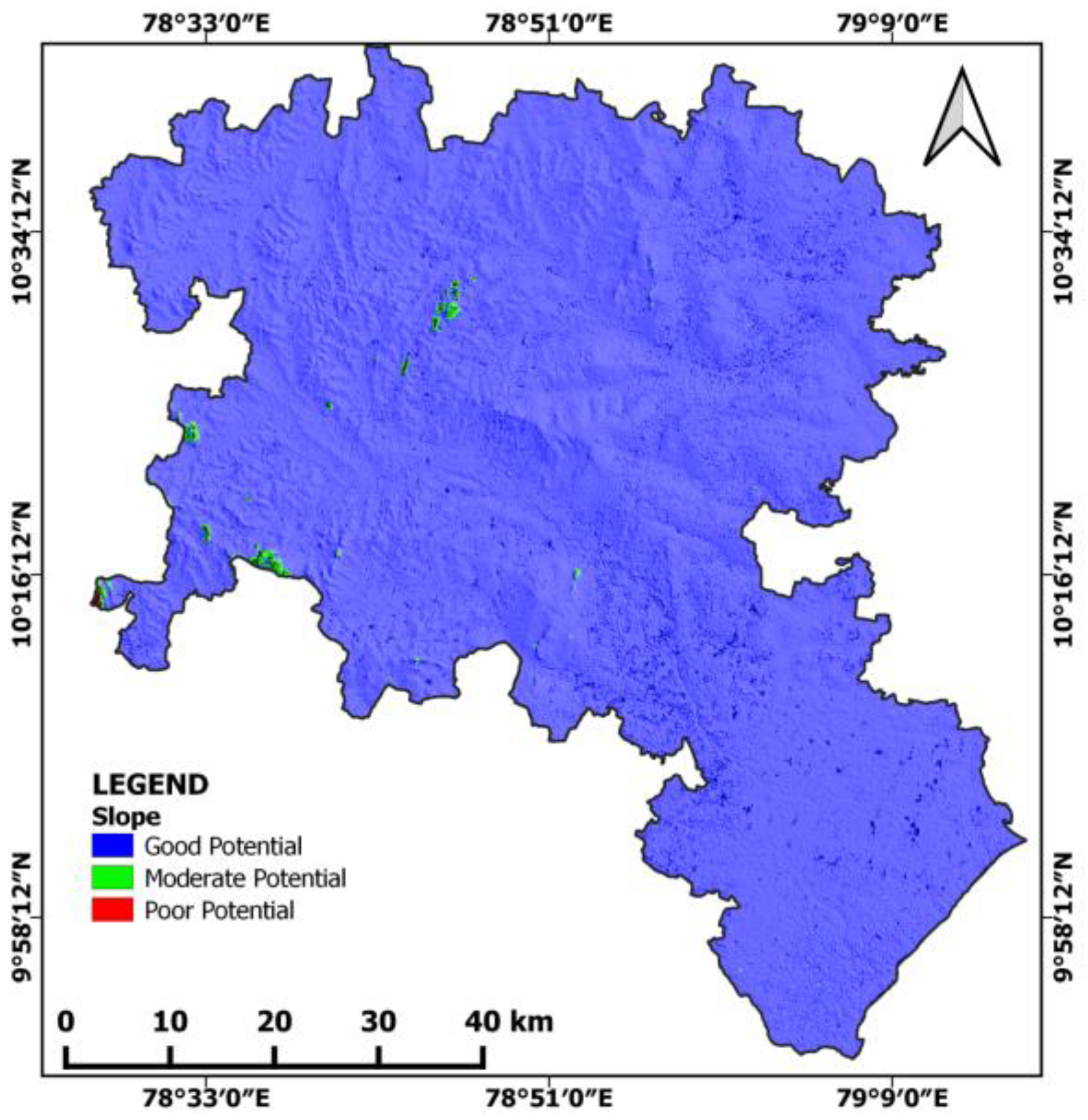
4.6. Degree of Slope
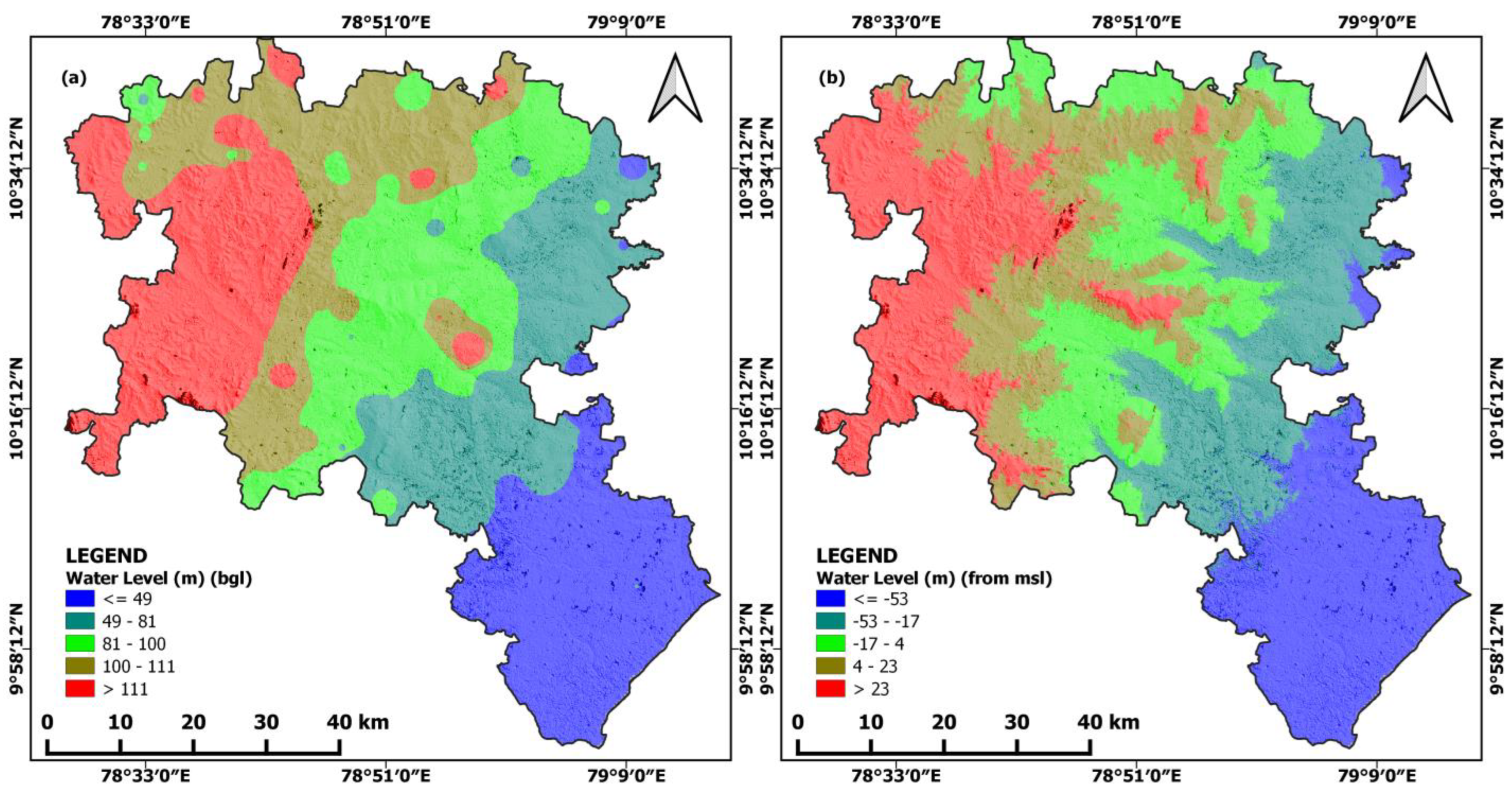
4.7. Ground Water Level
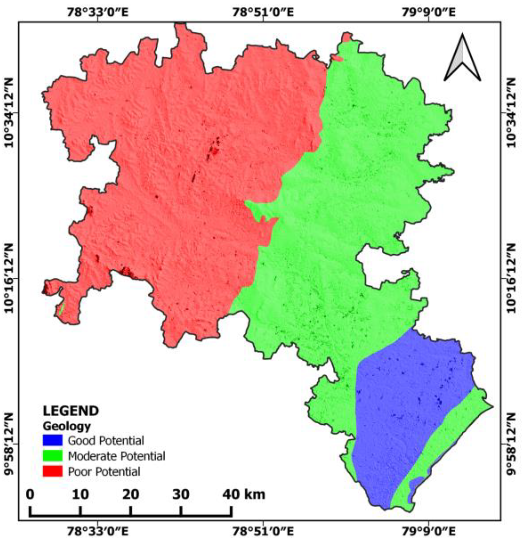
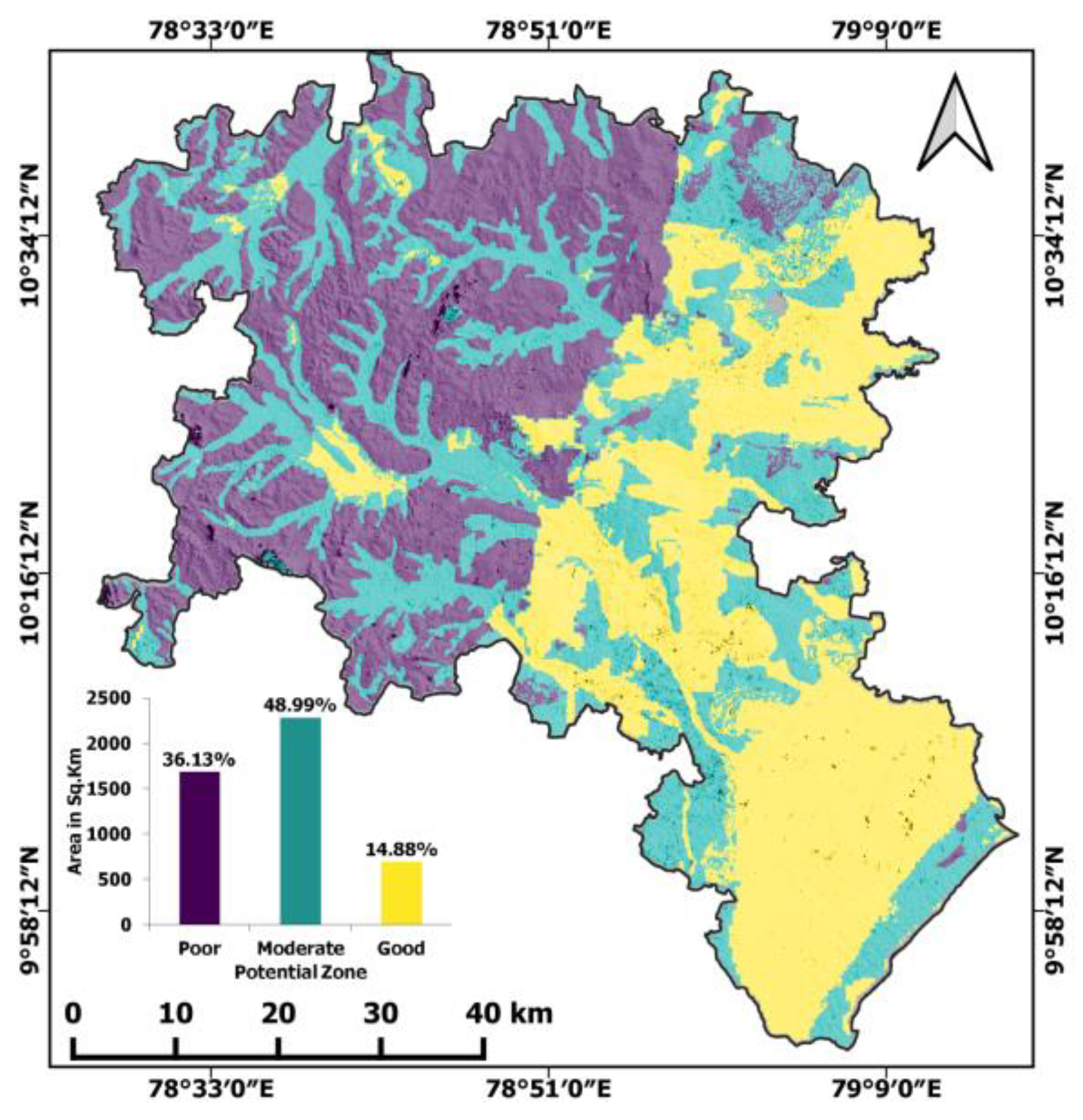
4.8. GWPZ Map
4.9. Validation of GWPZ Map
5. Conclusions
Author Contributions
Funding
Data Availability Statement
Conflicts of Interest
References
- Arnell, N.W.; Reynard, N.S. Impact of Climatic Variability and Change on River Flow Regimes in the United Kingdom: Report to Department of the Environment, Water Directorate; Institute of Hydrology, NERC: Wallingford, UK, 1990; 163p. [Google Scholar]
- William, A.J.; Vaux, H., Jr. The role of science in solving the world’s emerging water problems. Proc. Natl. Acad. Sci. USA 2005, 102, 157155720. [Google Scholar] [CrossRef] [Green Version]
- Muruganantham, A.; Sivakumar, K.; Kongeswaran, T.; Prabakaran, K.; Bangaru Priyanga, S.; Karikalan, R.; Agastheeswaran, V.; Perumal, V. Hydrogeochemical Analysis for Groundwater Suitability Appraisal in Sivagangai, an Economically Backward District of Tamil Nadu. J. Geol. Soc. India 2021, 97, 789–798. [Google Scholar] [CrossRef]
- Kongeswaran, T.; Sivakumar, K. Application of Remote Sensing and GIS in Floodwater Harvesting for Groundwater Development in the Upper Delta of Cauvery River Basin, Southern India. In Water Resources Management and Sustainability, Advances in Geographical and Environmental Sciences; Pankaj, K., Gaurav, K.N., Manish Kumar, S., Anju, S., Eds.; Springer Nature: Berlin/Heidelberg, Germany, 2022; pp. 257–280. [Google Scholar] [CrossRef]
- Sivakumar, K.; Prabakaran, K.; Saravanan, P.K.; Muthusamy, S.; Kongeswaran, T.; Muruganantham, A.; Gnanachandrasamy, G. Agriculture Drought Management in Ramanathapuram District of Tamil Nadu, India. J. Clim. Change 2022, 8, 59–65. [Google Scholar] [CrossRef]
- Muruganantham, A.; Sivakumar, K.; Prabakaran, K.; Kongeswaran, T.; Venkatramanan, S.; Bangaru, P.S.; Agastheeswaran, V.; Perumal, V. Role of GIS in deciphering hydrogeochemical processes and quality in Pudukottai district, Tamil Nadu, India. Environ. Earth Sci. 2022, 81, 445. [Google Scholar] [CrossRef]
- Chandra, S.; Auken, E.; Maurya, P.K.; Ahmed, S.; Verma, S.K. Large Scale Mapping of Fractures and Groundwater Pathways in Crystalline Hardrock By AEM. Sci Rep. 2019, 9, 398. [Google Scholar] [CrossRef] [Green Version]
- Saaty, T.L. A scaling method for priorities in hierarchical structures. J. Math. Psychol. 1977, 15, 234–281. [Google Scholar] [CrossRef]
- Saaty, T.L. The Analytic Hierarchy Process; McGraw-Hill: New York, NY, USA, 1980. [Google Scholar]
- Saaty, T.L. Axiomatic foundation of the Analytic Hierarchy Process. Manag. Sci. 1986, 32, 841–855. [Google Scholar] [CrossRef]
- Rozann, W. The Analytic Hierarchy Process—What It Is and How It Is Used. Math. Model. 1987, 9, 161–176. [Google Scholar] [CrossRef] [Green Version]
- Saaty, T.L. An exposition of the AHP in reply to the paper Remarks on the analytic hierarchy process. Manag. Sci. 1990, 36, 259–268. [Google Scholar] [CrossRef]
- Kumar, A.; Sah, B.; Singh, A.; Deng, Y.; He, X.; Kumar, P.; Bansal, R. A review of multi criteria decision making (MCDM) towards sustainable renewable energy development. Renew. Sustain. Energy Rev. 2017, 69, 596–609. [Google Scholar] [CrossRef]
- Sivakumar, K.; Shanmugasundaram, A.; Jayaprakash, M.; Prabakaran, K.; Muthusamy, S.; Ramachandran, A.; Venkatramanan, S.; Selvam, S. Causes of heavy metal contamination in groundwater of Tuticorin industrial block, Tamil Nadu, India. Environ. Sci. Pollut. Res. 2021, 28, 18651–18666. [Google Scholar] [CrossRef]
- Prabakaran, K.; Sivakumar, K.; Aruna, C. Use of GIS-AHP tools for potable groundwater potential zone investigations-a case study in Vairavanpatti rural area, Tamil Nadu, India. Arab. J. Geosci. 2020, 13, 866. [Google Scholar] [CrossRef]
- Ramachandran, A.; Sivakumar, K.; Shanmugasundharam, A.; Sangunathan, U.; Krishnamurthy, R.R. Evaluation of potable groundwater zones identification based on WQI and GIS techniques in Adyar River basin, Chennai, Tamilnadu, India. Acta Ecol. Sin. 2020, 41, 285–295. [Google Scholar] [CrossRef]
- Venkatramanan, S.; Chung, S.Y.; Ramkumar, T.; Gnanachandrasamy, G.; Vasudevan, S. A multivariate statistical approaches on physicochemical characteristics of ground water in and around Nagapattinam district, Cauvery deltaic region of Tamil Nadu, India. Earth Sci. Res. J. 2013, 17, 97–103. [Google Scholar]
- Hilletofth, P.; Sequeira, M.; Adlemo, A. Three novel fuzzy logic concepts applied to reshoring decision-making. Expert Syst. Appl. 2019, 126, 133–143. [Google Scholar] [CrossRef]
- Sivakumar, K.; Prabakaran, K.; Venkatramanan, S.; Chung, S.Y.; Kongeswaran, T.; Muruganantham, A.; Sathish, S.; Ho-Na, S. Hydrogeochemical Survey along the Northern Coastal Region of Ramanathapuram District, Tamilnadu, India. Appl. Sci. 2022, 12, 5595. [Google Scholar] [CrossRef]
- Fathy, A.; Karem, M.; Mohamed, A. Groundwater potential mapping using GIS, linear weighted combination techniques and geochemical processes identification, west of the Qena area, Upper Egypt. J. Taibah Univ. Sci. 2020, 14, 1350–1362. [Google Scholar] [CrossRef]
- Saaty, T.L.; Takizawa, M. Dependence and independence: From linear hierarchies to nonlinear networks. Eur. J. Oper. Res. 1986, 26, 229–237. [Google Scholar] [CrossRef]
- Agastheeswaran, V.; Udayaganesan, P.; Sivakumar, K.; Venkatramanan, S.; Prasanna, M.V.; Selvam, S. Identification of groundwater potential zones using geospatial approach in Sivagangai district, South India. Arab. J. Geosci. 2021, 14, 8. [Google Scholar] [CrossRef]
- Kaliraj, S.; Chandrasekar, N.; Magesh, N.S. Identification of potential groundwater recharge zones in Vaigai upper basin, Tamil Nadu, using GIS-based analytical hierarchical process (AHP) technique. Arab. J. Geosci. 2014, 7, 1385–1401. [Google Scholar] [CrossRef]
- Senapati, U.; Das, T. Assessment of basin-scale groundwater potentiality mapping in drought-prone upper Dwarakeshwar River basin, West Bengal, India, using GIS-based AHP techniques. Arab. J. Geosci. 2021, 14, 960. [Google Scholar] [CrossRef]
- Ahmed, A.; Alrajhi, A.; Alquwaizany, A.S. Identification of Groundwater Potential Recharge Zones in Flinders Ranges, South Australia Using Remote Sensing, GIS, and MIF Techniques. Water 2021, 13, 2571. [Google Scholar] [CrossRef]
- Minh, H.V.T.; Ram, A.; Pankaj, K.; Dat, Q.T.; Tran, V.T.; Hari, C.B.; Masaaki, K. Groundwater Quality Assessment Using Fuzzy-AHP in a Giang Province of Vietnam. Geosciences 2019, 9, 330. [Google Scholar] [CrossRef] [Green Version]
- Chandrasekar, N.; Prince, J. Delineation of groundwater potential zones in Theni district, Tamil Nadu, using remote sensing, GIS and MIF techniques. Geosci. Front. 2012, 3, 189–196. [Google Scholar] [CrossRef] [Green Version]
- Gdoura, K.; Anane, M.; Jellali, S. Geospatial and AHP-multicriteria analyses to locate and rank suitable sites for groundwater recharge with reclaimed water. Resour. Conserv. Recycl. 2015, 104, 19–30. [Google Scholar] [CrossRef]
- Shashank, S.; Arvind, C.P. Delineation of groundwater potential zone in hard rock terrain of India using remote sensing, geographical information system (GIS) and analytic hierarchy process (AHP) techniques. Geocarto Int. 2015, 30, 402–421. [Google Scholar] [CrossRef]
- Tanveer, D.; Nachiketa, R.; Aadil, B. Delineation of potential groundwater recharge zones using analytical hierarchy process (AHP). Geol. Ecol. Landsc. 2021, 5, 292–307. [Google Scholar] [CrossRef] [Green Version]
- Mallick, J.; Khan, R.A.; Ahmed, M.; Alqadhi, S.D.; Alsubih, M.; Falqi, I.; Hasan, M.A. Modeling Groundwater Potential Zone in a Semi-Arid Region of Aseer Using Fuzzy-AHP and Geoinformation Techniques. Water 2019, 11, 2656. [Google Scholar] [CrossRef] [Green Version]
- Cabrera-Barona, P.; Ghorbanzadeh, O. Comparing Classic and Interval Analytical Hierarchy Process Methodologies for Measuring Area-Level Deprivation to Analyze Health Inequalities. Int. J. Environ. Res. Public Health 2018, 15, 140. [Google Scholar] [CrossRef] [Green Version]
- Navane, V.S.; Sahoo, S.N. Identification of groundwater recharge sites in Latur district of Maharashtra in India based on remote sensing, GIS and multi-criteria decision tools. Water Environ. J. 2020, 35, 544–559. [Google Scholar] [CrossRef]
- Haile, M.; Yadeta, J.; Gambe, L. Delineation of groundwater potential zones using geo-spatial and AHP techniques: Ambo area, Blue Nile Basin, Ethiopia. Sustain. Water Resour. Manag. 2022, 8, 36. [Google Scholar] [CrossRef]
- Song, B.; Kang, S. A Method of Assigning Weights Using a Ranking and Nonhierarchy Comparison. Adv. Decis. Sci. 2016, 2016, 8963214. [Google Scholar] [CrossRef] [Green Version]
- Recep, Ç. Evaluation of Groundwater Potential by GIS-Based Multicriteria Decision Making as a Spatial Prediction Tool: Case Study in the Tigris River Batman-Hasankeyf Sub-Basin, Turkey. Water 2019, 11, 2630. [Google Scholar] [CrossRef] [Green Version]
- Chakraborty, B.; Roy, S.; Bera, A.; Adhikary, P.P.; Bera, B.; Sengupta, D.; Bhunia, G.S.; Shit, P.K. Groundwater vulnerability assessment using GIS-based DRASTIC model in the upper catchment of Dwarakeshwar river basin, West Bengal, India. Environ. Earth Sci. 2022, 81, 112085. [Google Scholar] [CrossRef]
- Thangavelu, M.; Kumanan, C. Remote Sensing and GIS Based Study of Land Suitability Evaluation in Coastal Domains of Pudukkottai District, Tamil Nadu, India. Int. J. Geol. Earth Sci. 2016, 2, 25–40. [Google Scholar]
- Premkumar, M.; Kongeswaran, T.; Sivakumar, K.; Muruganantham, A.; Muthuramalingam, R.; Chandramohan, S.; Vasanthavigar, M. Spit Evolution and Shoreline Changes Along Manamelkudi Coast Using Geo-Spatial Techniques and Statistical Approach. J. Clim. Change 2022, 8, 59–67. [Google Scholar] [CrossRef]
- Yuvaraj, R.M.; Rajeswari, M. GIS Based Soil Fertility Status of Pudukkottai District. Int. J. Interdiscip. Res. Innov. 2020, 6, 25–35. [Google Scholar]
- Ramachandran Muthulakshmi, Y. Geo-spatial analysis of irrigation water quality of Pudukkottai district. Appl. Water Sci. 2020, 10, 82. [Google Scholar] [CrossRef] [Green Version]
- Gunasekaran, S.; Ramasamy, S.M.; Palanivel, K.; Saravanavel, J.; Selvakumar, R. Remote Sensing and GIS Based 3d Visualization of Groundwater Level Modification and Their Signatures: Pudukkottai District, Tamil Nadu. Asian J. Appl. Sci. 2014, 7, 403–413. [Google Scholar] [CrossRef] [Green Version]
- Yuvaraj, R. M Assessment of Land Use/Land Cover and Its Dynamic Using Geospatial Techniques in Pudukkottai District of Tamil Nadu. Environ. Ecol. Res. 2020, 8, 85–99. [Google Scholar] [CrossRef]
- Monisha, N.; Balasubramaniam, P.; Janaki, D.; Ramesh, T.; Mahendran, P.P. Assessment of groundwater quality and mapping in coastal blocks of Pudukkottai district, Tamil Nadu. Pharma Innov. J. 2021, SP-10, 777–781. [Google Scholar]
- Pinto, D.; Shrestha, S.; Babel, M.S.; Ninsawat, S. Delineation of groundwater potential zones in the Comoro watershed, Timor Leste using GIS, remote sensing and analytic hierarchy process (AHP) technique. Appl. Water Sci. 2017, 7, 503–519. [Google Scholar] [CrossRef] [Green Version]
- Rajasekhara, M.; Sudarsana, R.G.; Sreenivasulub, Y.; Siddi, R. Delineation of groundwater potential zones in semi-arid region of Jilledubanderu river basin, Anantapur District, Andhra Pradesh, India using fuzzy logic, AHP and integrated fuzzy-AHP approaches. HydroResearch 2019, 2, 97–108. [Google Scholar] [CrossRef]
- Sener, E.; Davraz, A. Assessment of groundwater vulnerability based on a modified DRASTIC model, GIS and an analytic hierarchy process (AHP) method: The case of Egirdir Lake basin (Isparta, Turkey). Hydrogeol. J. 2013, 21, 701–714. [Google Scholar] [CrossRef]
- Pathmanandakumar, V.; Thasarathan, N.; Ranagalage, M. An approach to delineate potential groundwater zones in Kilinochchi district, Sri Lanka, using GIS techniques. ISPRS Int. J. Geo-Inf. 2021, 10, 730. [Google Scholar] [CrossRef]
- Mengistu, T.D.; Chang, S.W.; Kim, I.H.; Kim, M.G.; Chung, I.M. Determination of Potential Aquifer Recharge Zones Using Geospatial Techniques for Proxy Data of Gilgel Gibe Catchment, Ethiopia. Water 2022, 14, 1362. [Google Scholar] [CrossRef]
- Sajil Kumar, P.J.; Elango, L.; Schneider, M. GIS and AHP Based Groundwater Potential Zones Delineation in Chennai River Basin (CRB), India. Sustainability 2022, 14, 1830. [Google Scholar] [CrossRef]


| Layers | Geology | Geomorphology | Soil | Drainage Density | Lineament Density | Slope | Water Level |
|---|---|---|---|---|---|---|---|
| Geology | 1.000 | 3.000 | 4.000 | 5.000 | 6.000 | 7.000 | 8.000 |
| Geomorphology | 0.333 | 1.000 | 3.000 | 4.000 | 5.000 | 6.000 | 7.000 |
| Soil | 0.250 | 0.333 | 1.000 | 3.000 | 4.000 | 5.000 | 6.000 |
| Drainage density | 0.200 | 0.250 | 0.333 | 1.000 | 3.000 | 4.000 | 5.000 |
| Lineament density | 0.167 | 0.200 | 0.250 | 0.333 | 1.000 | 3.000 | 4.000 |
| Slope | 0.143 | 0.167 | 0.200 | 0.250 | 0.333 | 1.000 | 3.000 |
| Water level | 0.125 | 0.143 | 0.167 | 0.200 | 0.250 | 0.333 | 1.000 |
| SUM | 2.218 | 5.093 | 8.950 | 13.78 | 19.58 | 26.33 | 34.00 |
| Layers | Geology | Geomorphology | Soil | Drainage Density | Lineament Density | Slope | Water Level | Weights |
|---|---|---|---|---|---|---|---|---|
| Geology | 0.451 | 0.589 | 0.447 | 0.363 | 0.306 | 0.266 | 0.235 | 0.404 |
| Geomorphology | 0.150 | 0.196 | 0.335 | 0.290 | 0.255 | 0.228 | 0.206 | 0.243 |
| Soil | 0.113 | 0.065 | 0.112 | 0.218 | 0.204 | 0.190 | 0.176 | 0.150 |
| Drainage density | 0.090 | 0.049 | 0.037 | 0.073 | 0.153 | 0.152 | 0.147 | 0.092 |
| Lineament density | 0.075 | 0.039 | 0.028 | 0.024 | 0.051 | 0.114 | 0.118 | 0.055 |
| Slope | 0.064 | 0.033 | 0.022 | 0.018 | 0.017 | 0.038 | 0.088 | 0.032 |
| Water level | 0.056 | 0.028 | 0.019 | 0.015 | 0.013 | 0.013 | 0.029 | 0.024 |
| Eigen vector | 1.000 | 1.000 | 1.000 | 1.000 | 1.000 | 1.000 | 1.000 | 1.000 |
| S.No | Parameter | Class | Score | Weights | Area % |
|---|---|---|---|---|---|
| 1 | Geology | Hornblende-biotite gneiss | 1 | 0.404 | 41.69 |
| 2 | Quartzo feldspathic gneiss | 1 | 0.404 | 0.02 | |
| 3 | Argillaceous sandstone with limestone | 3 | 0.404 | 0.30 | |
| 4 | Quartzite | 1 | 0.404 | 0.62 | |
| 5 | Laterite (Ferricrete) | 2 | 0.404 | 29.82 | |
| 6 | Charnockite | 1 | 0.404 | 0.21 | |
| 7 | Granite | 1 | 0.404 | 5.98 | |
| 8 | Clay | 2 | 0.404 | 0.13 | |
| 9 | Sandstone and shales | 2 | 0.404 | 0.46 | |
| 10 | Sand and silt | 3 | 0.404 | 0.50 | |
| 11 | Sand, Silt and Clay Partings | 2 | 0.404 | 6.85 | |
| 12 | Calc-granulite | 2 | 0.404 | 0.02 | |
| 13 | Clayey sand | 3 | 0.404 | 11.47 | |
| 14 | Sand, Silt with Clay | 2 | 0.404 | 2.29 | |
| 15 | Geomorphology | Shallow and moderately Weathered Pediplain | 3 | 0.243 | 66.50 |
| 16 | Upland | 1 | 0.243 | 10.11 | |
| 17 | Pediment | 1 | 0.243 | 0.81 | |
| 18 | Shallow Flood Plain | 3 | 0.243 | 4.90 | |
| 19 | Inselberg | 1 | 0.243 | 0.02 | |
| 20 | Linear Ridge/Dyke | 1 | 0.243 | 0.11 | |
| 21 | Bazada | 3 | 0.243 | 0.15 | |
| 22 | Pediment-InselbergComplex | 1 | 0.243 | 0.47 | |
| 23 | Pediplain Canal Command | 3 | 0.243 | 0.21 | |
| 24 | Channel bar | 1 | 0.243 | 0.17 | |
| 25 | Structural Hills | 1 | 0.243 | 0.06 | |
| 26 | Shallow alluvial plain | 2 | 0.243 | 13.43 | |
| 27 | Coastal Plain | 2 | 0.243 | 2.20 | |
| 28 | Lateritic | 3 | 0.243 | 0.04 | |
| 29 | Salt flat | 2 | 0.243 | 0.07 | |
| 30 | Brackish water creeks | 1 | 0.243 | 0.02 | |
| 31 | Beach ridge complex | 1 | 0.243 | 0.24 | |
| 32 | Dune complex | 3 | 0.243 | 0.05 | |
| 33 | Soil | Clay | 1 | 0.15 | 45.66 |
| 34 | Sandysilt | 1 | 0.15 | 24.13 | |
| 35 | Sandyclay | 2 | 0.15 | 22.47 | |
| 36 | ClayeySilt | 1 | 0.15 | 5.03 | |
| 37 | Sandstone | 3 | 0.15 | 2.66 | |
| 38 | Silty sand | 2 | 0.15 | 0.022 | |
| 39 | Drainage density | Low | 3 | 0.092 | 82.85 |
| 40 | Moderate | 2 | 0.092 | 15.47 | |
| 41 | High | 1 | 0.092 | 1.68 | |
| 42 | Lineament density | Low | 1 | 0.055 | 62.34 |
| 43 | Moderate | 2 | 0.055 | 26.06 | |
| 44 | High | 3 | 0.055 | 11.60 | |
| 45 | Slope | 0–4.5 (gentle slope) | 3 | 0.032 | 99.54 |
| 46 | 4.5–7.9 (moderate slope) | 2 | 0.032 | 0.44 | |
| 47 | >7.9 (steep slope) | 1 | 0.032 | 0.02 | |
| 48 | Water Level | <10 (Good) | 3 | 0.024 | 6.56 |
| 49 | 10–50 (Moderate) | 2 | 0.024 | 17.51 | |
| 50 | >50 (Poor) | 1 | 0.024 | 75.9 |
| Zone | Description | Area in km2 | Area in % |
|---|---|---|---|
| 1 | Poor potential zone | 1684.8 | 36.13 |
| 2 | Moderate potential zone | 2284.5 | 48.99 |
| 3 | Good potential zone | 693.7 | 14.88 |
| Total | 4663.0 | 100 | |
| Thematic Layer | AHP Weight | Effective Weight | ||
|---|---|---|---|---|
| Minimum | Maximum | Mean | ||
| Geology | 0.404 | 1.90 | 5.71 | 3.53 |
| Geomorphology | 0.243 | 1.14 | 3.43 | 2.10 |
| Soil | 0.150 | 0.71 | 2.12 | 1.18 |
| Drainage density | 0.092 | 0.43 | 1.30 | 0.87 |
| Lineament density | 0.055 | 0.26 | 0.78 | 0.52 |
| Slope | 0.032 | 0.15 | 0.45 | 0.30 |
| Water Level | 0.024 | 0.11 | 0.34 | 0.23 |
| Zone | Description | Total Area (km2) | Well Count | Well Density |
|---|---|---|---|---|
| 1 | Poor potential zone | 1684.8 | 30 | 56 |
| 2 | Moderate potential zone | 2284.5 | 37 | 62 |
| 3 | Good potential zone | 693.7 | 13 | 53 |
| Total | 4663.0 | 80 | 58 | |
Disclaimer/Publisher’s Note: The statements, opinions and data contained in all publications are solely those of the individual author(s) and contributor(s) and not of MDPI and/or the editor(s). MDPI and/or the editor(s) disclaim responsibility for any injury to people or property resulting from any ideas, methods, instructions or products referred to in the content. |
© 2023 by the authors. Licensee MDPI, Basel, Switzerland. This article is an open access article distributed under the terms and conditions of the Creative Commons Attribution (CC BY) license (https://creativecommons.org/licenses/by/4.0/).
Share and Cite
Arumugam, M.; Kulandaisamy, P.; Karthikeyan, S.; Thangaraj, K.; Senapathi, V.; Chung, S.Y.; Muthuramalingam, S.; Rajendran, M.; Sugumaran, S.; Manimuthu, S. An Assessment of Geospatial Analysis Combined with AHP Techniques to Identify Groundwater Potential Zones in the Pudukkottai District, Tamil Nadu, India. Water 2023, 15, 1101. https://doi.org/10.3390/w15061101
Arumugam M, Kulandaisamy P, Karthikeyan S, Thangaraj K, Senapathi V, Chung SY, Muthuramalingam S, Rajendran M, Sugumaran S, Manimuthu S. An Assessment of Geospatial Analysis Combined with AHP Techniques to Identify Groundwater Potential Zones in the Pudukkottai District, Tamil Nadu, India. Water. 2023; 15(6):1101. https://doi.org/10.3390/w15061101
Chicago/Turabian StyleArumugam, Muruganantham, Prabakaran Kulandaisamy, Sivakumar Karthikeyan, Kongeswaran Thangaraj, Venkatramanan Senapathi, Sang Yong Chung, Subagunasekar Muthuramalingam, Muthuramalingam Rajendran, Sathish Sugumaran, and Siva Manimuthu. 2023. "An Assessment of Geospatial Analysis Combined with AHP Techniques to Identify Groundwater Potential Zones in the Pudukkottai District, Tamil Nadu, India" Water 15, no. 6: 1101. https://doi.org/10.3390/w15061101