
Driving Factors and Trend Prediction for Annual Sediment Transport in the Upper and Middle Reaches of the Yellow River from 2001 to 2020

Abstract
:1. Introduction
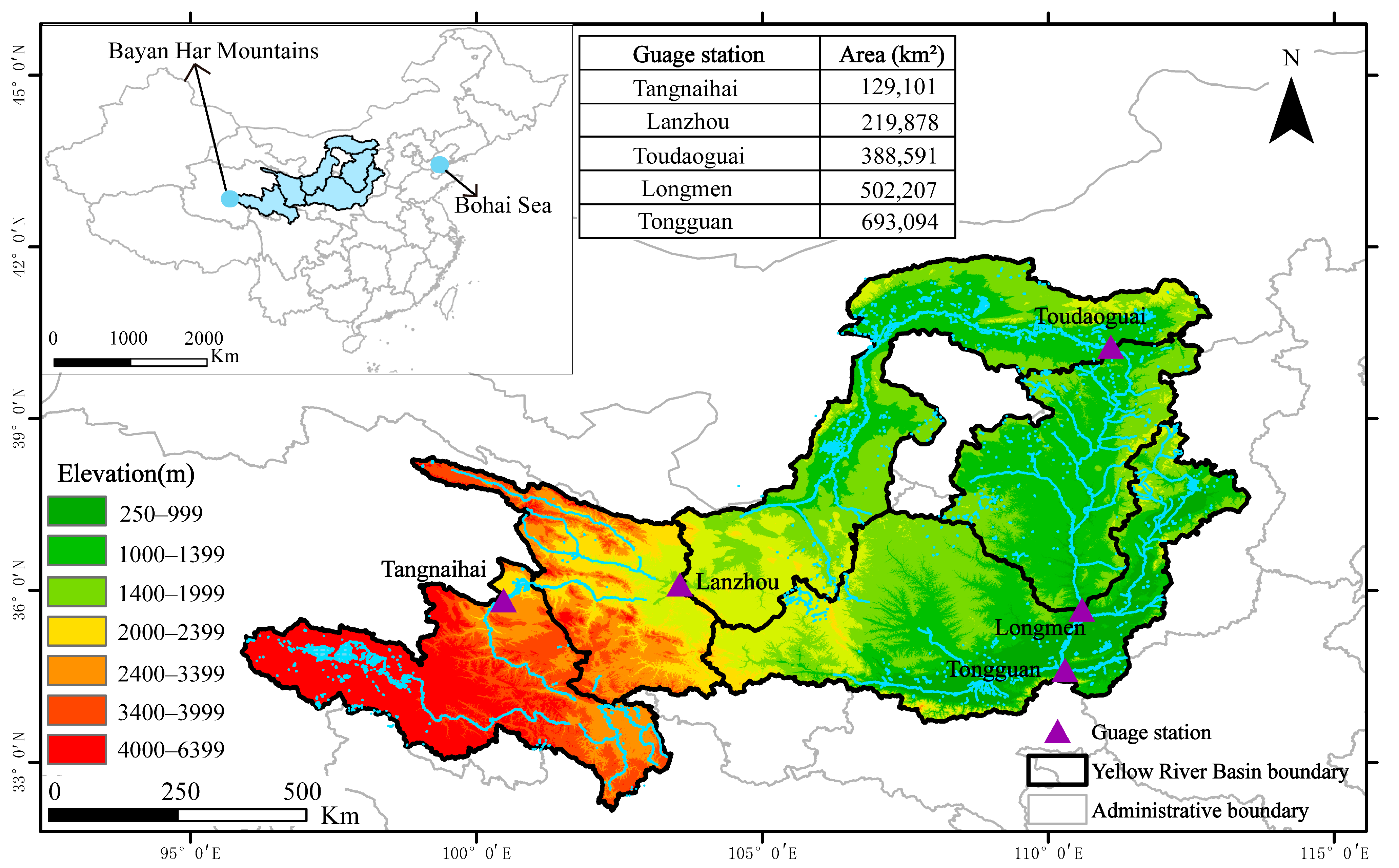
2. Study Area
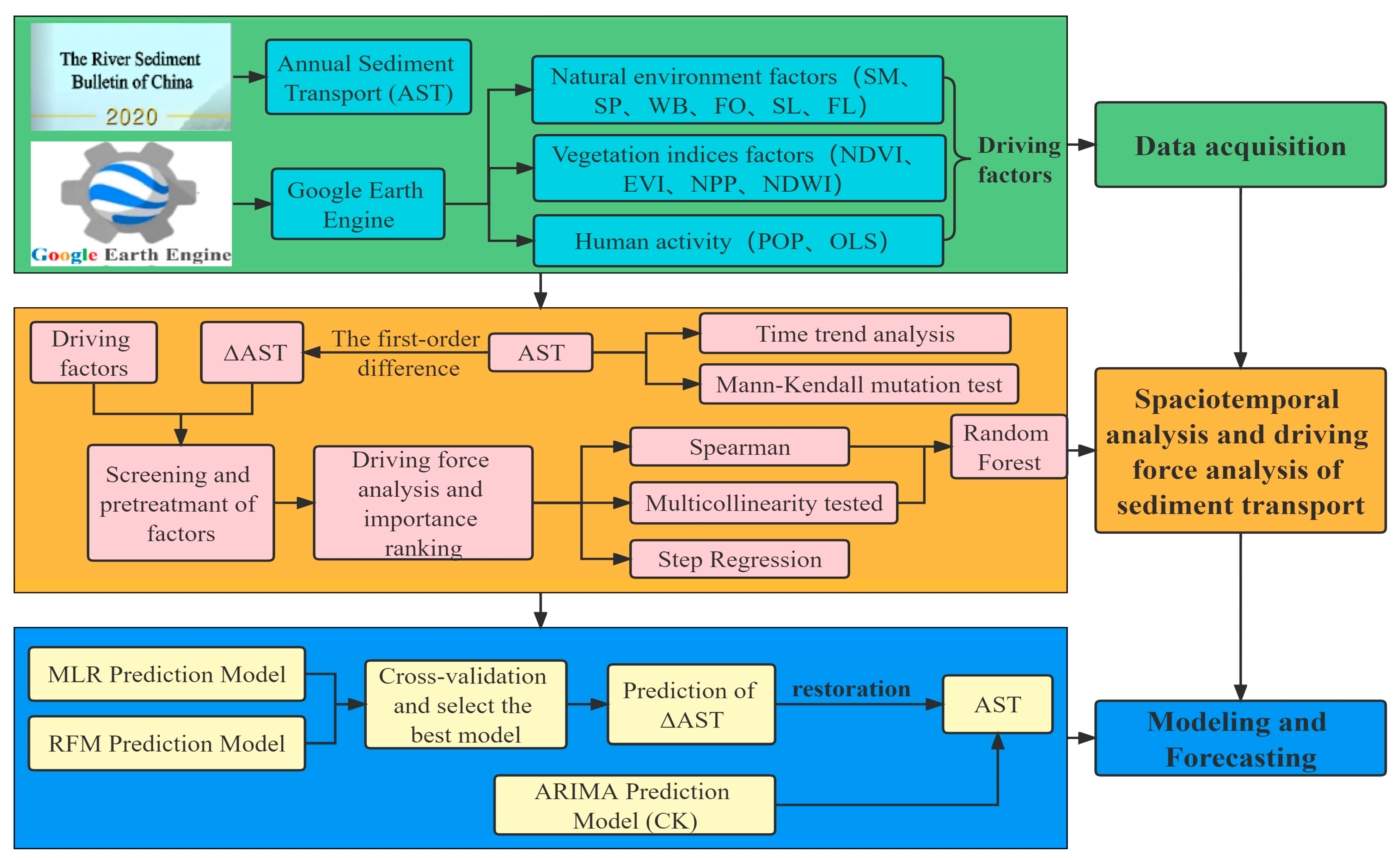
3. Materials and Methods
3.1. Data
3.2. Research Methods
3.2.1. Mann–Kendall Mutational Test
3.2.2. Driving Force Analysis Method
- (1)
- Spearman correlation analysis
- (a)
- The value of the correlation (the Spearman correlation between the driving factors). A high correlation value between the two driving factors shows that there is a linear relationship, and indicates that there may be a problem of collinearity [22].
- (b)
- The value of the variance inflation factor (VIF) is used as a criterion to detect the presence of multicollinearity in a multiple linear regression. When the value of the VIF is greater than 3, there may be a problem of multicollinearity [23].
- (2)
- Linear model
- (3)
- Nonlinear model
3.2.3. Accuracy Validation and Prediction of Models
- (1)
- Model accuracy validation
- (2)
- Prediction of AST
4. Results
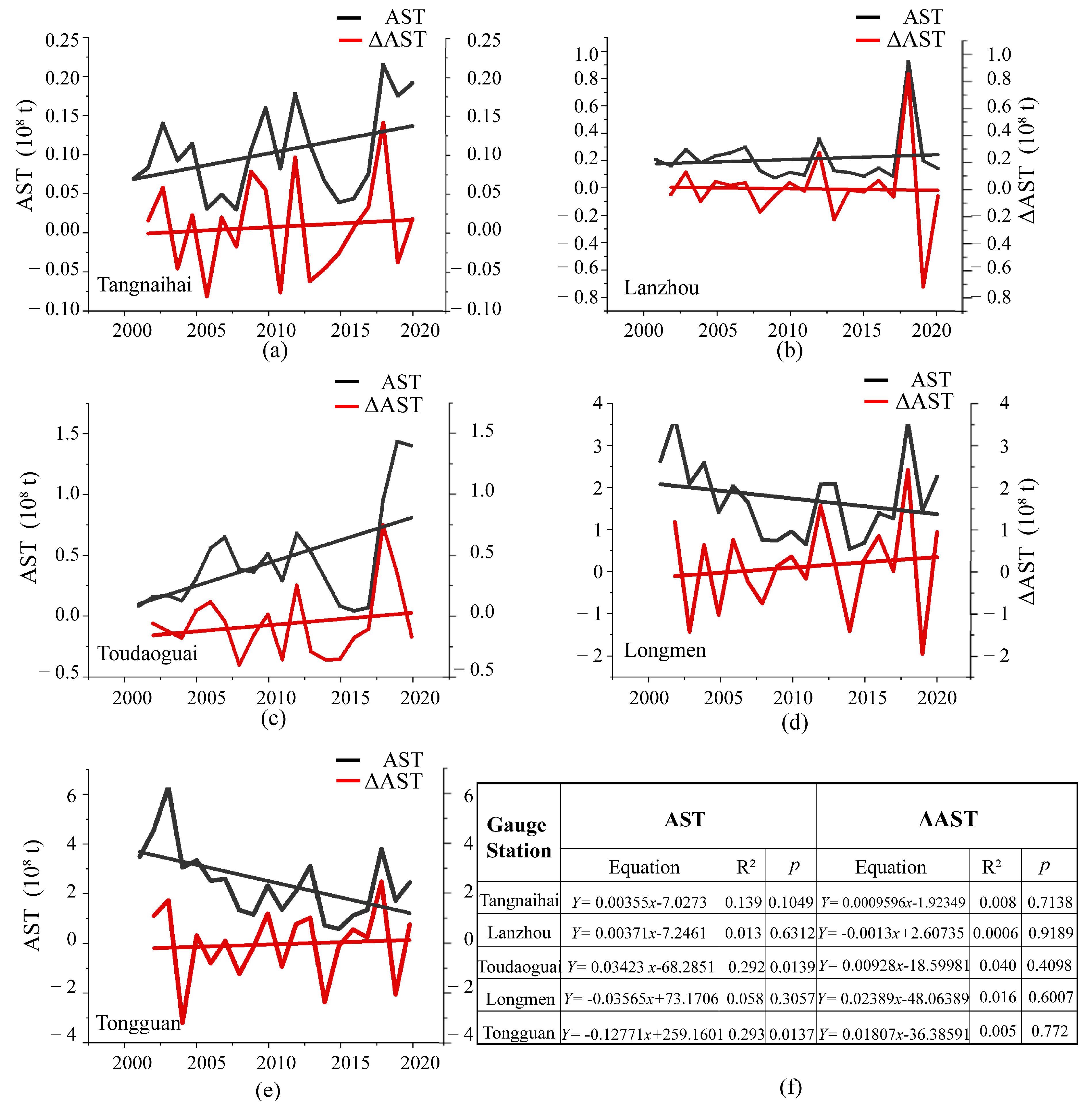
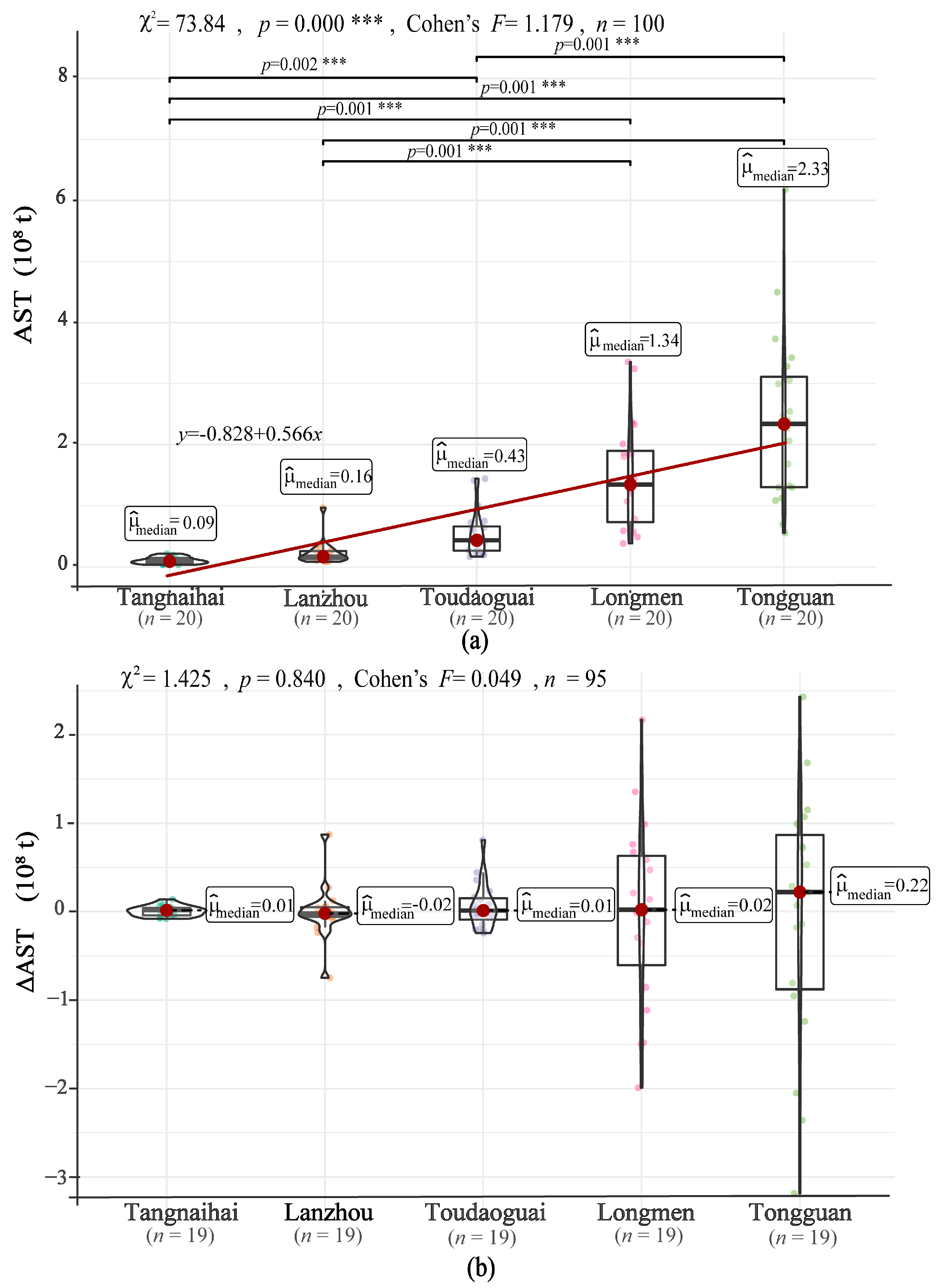
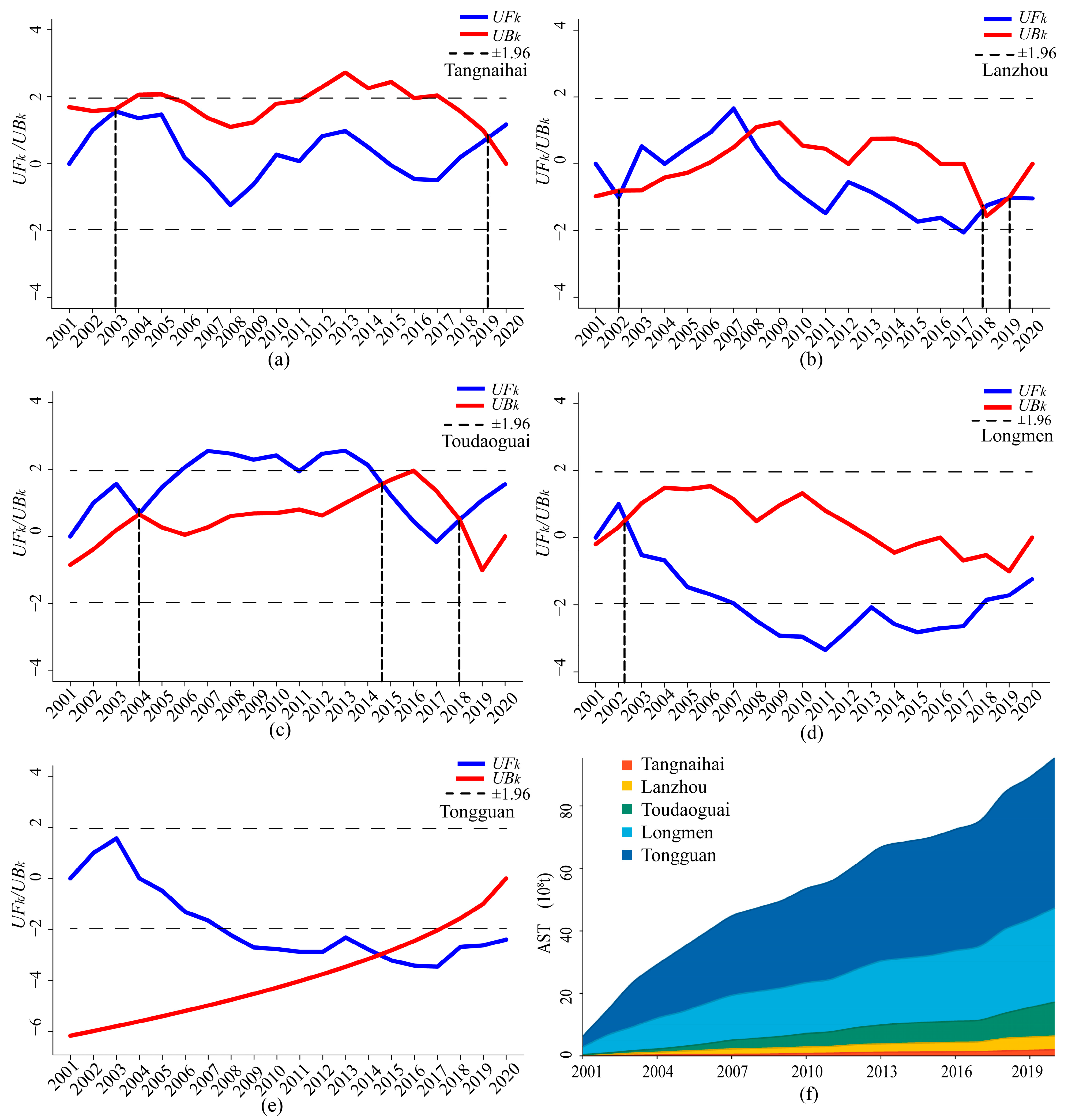
4.1. Analysis of Variation Trend and Mutation of the AST
4.2. Driving Force Analysis
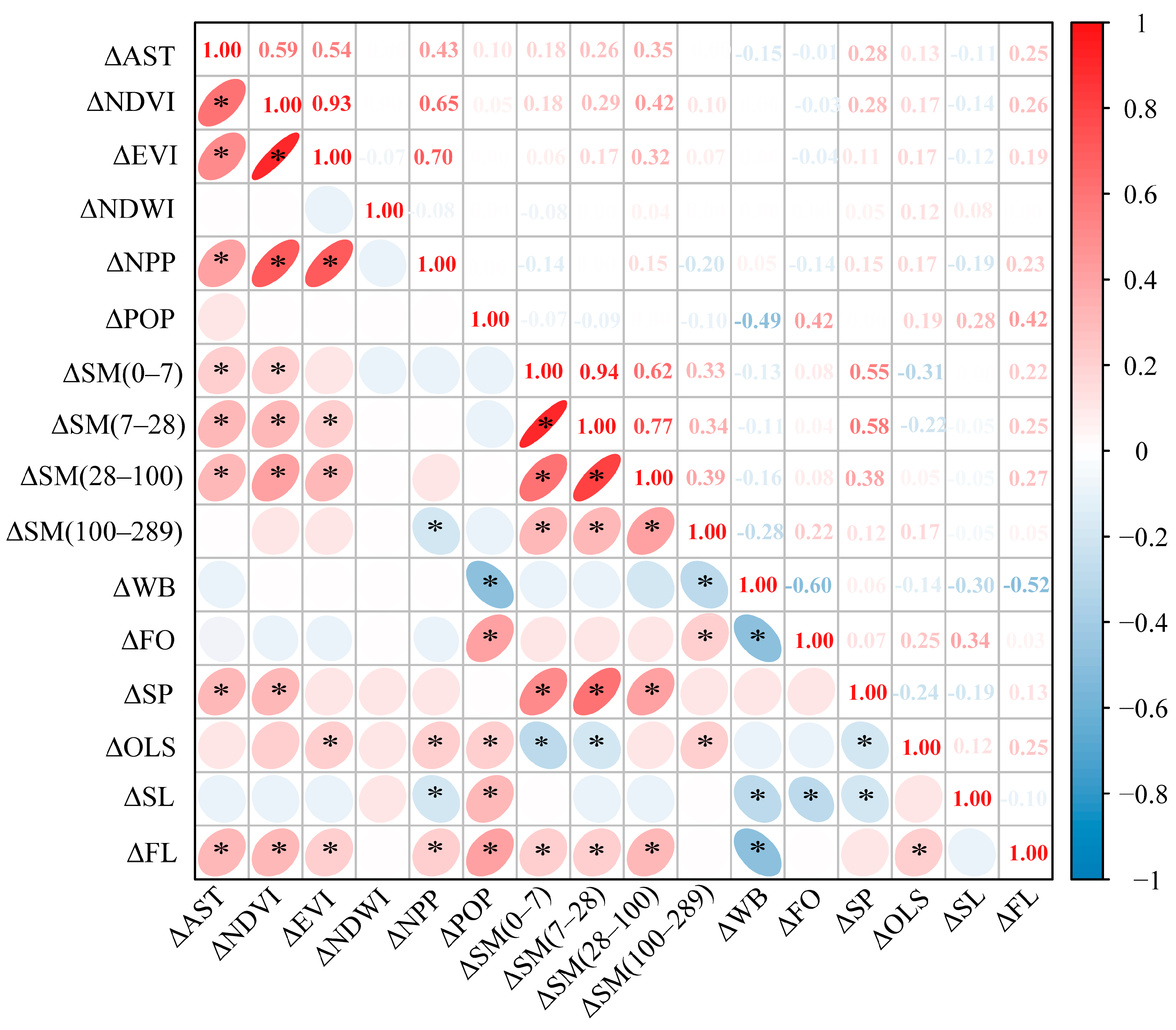
4.2.1. Spearman Correlation Analysis
4.2.2. Multicollinearity Test
4.2.3. Stepwise Regression
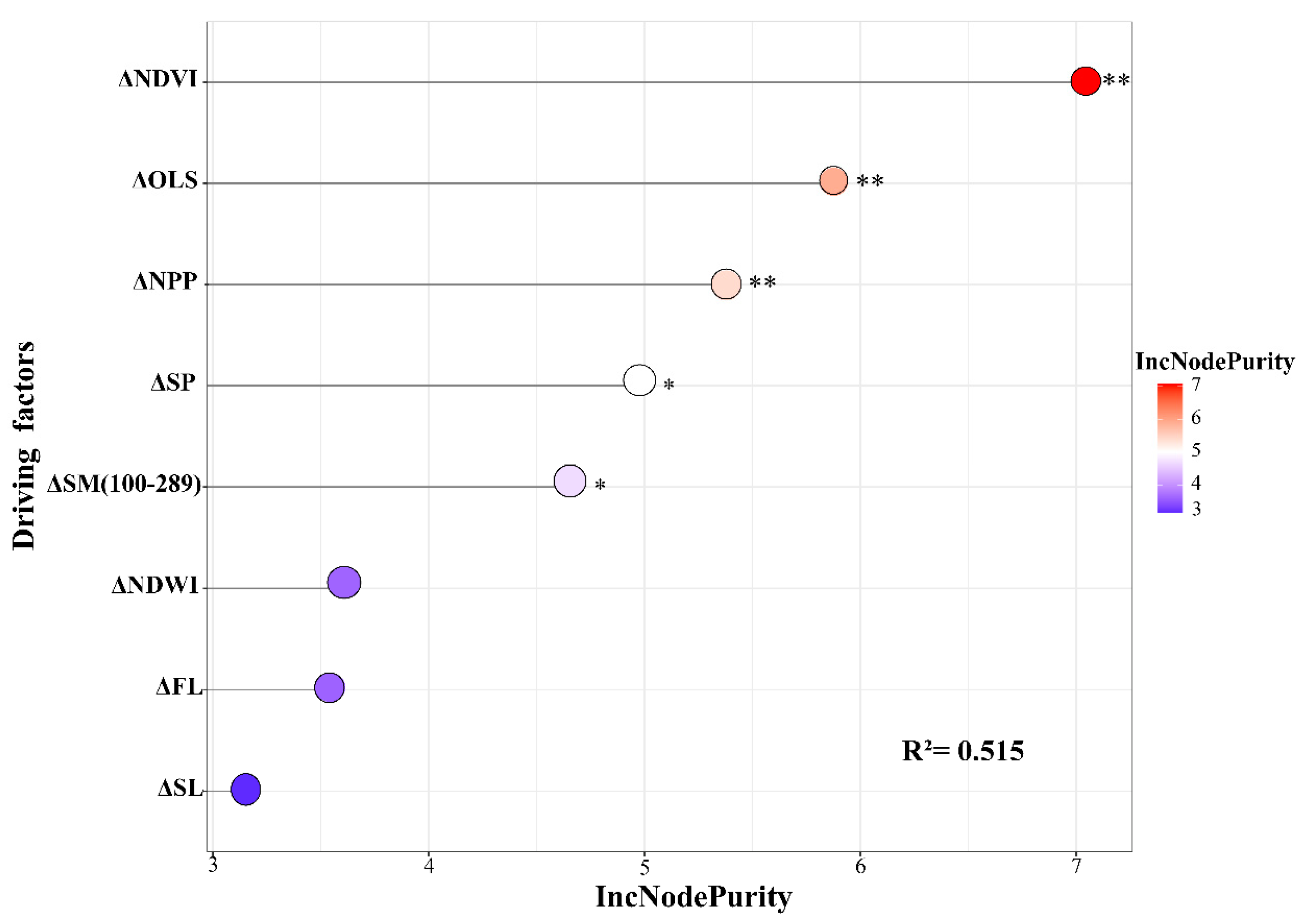
4.2.4. RFM Regression
4.3. Modeling and Prediction
4.3.1. Cross–Validation and Selection of the Model
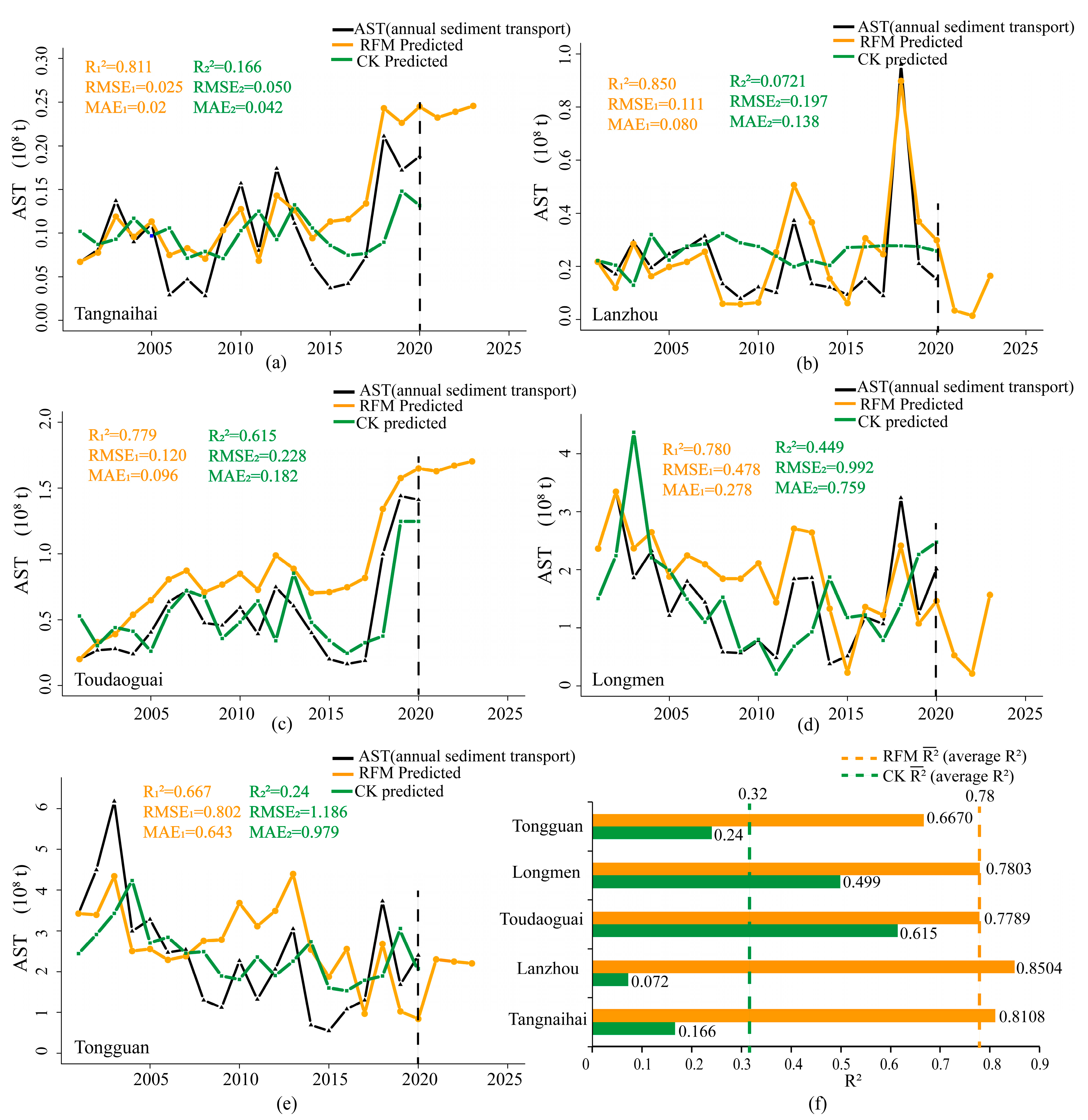
4.3.2. Prediction of AST
5. Discussion
5.1. Changes in AST in the UMRYR
5.2. Analysis of Driving Force of ΔAST and Modeling
5.3. Limitations and Future Work
6. Conclusions
Author Contributions
Funding
Data Availability Statement
Conflicts of Interest
References
- Shi, F.C.; Zhang, R. Analysis and understanding of the reasons for the sharp decrease of water and sediment in the yellow river in recent years. Yellow River 2013, 35, 1–3. [Google Scholar]
- Liu, C.M.; Wei, H.S.; Zhang, Y.Q.; Tian, W.; Luan, J.K. Attribution Analysis of Runoff Variation in the Main Stream of the Yellow River and Discussion on Related Problems. Yellow River 2021, 43, 1–6. [Google Scholar]
- Jan, V.; Rob, H.; Glenn, N.; Darius, C. Detecting trend and seasonal changes in satellite image time series. Remote Sens. Environ. 2009, 114, 106–115. [Google Scholar]
- Wang, H.; Yang, Z.; Saito, Y.; Liu, J.P.; Sun, X.; Wang, Y. Stepwise decreases of the Huanghe (Yellow River) sediment load (1950–2005): Impacts of climate change and human activities. Glob. Planet Chang. 2007, 57, 331–354. [Google Scholar]
- Shi, H.L.; Hu, C.H.; Wang, Y.G.; Hu, J. Trend analysis of water and sediment variation in the yellow river basin and its causes. Yellow River 2014, 36, 1–5. [Google Scholar]
- Hu, C.H.; Chen, X.J.; Chen, J.G. Spatial distribution and its variation process of sedimentation in Yellow River. J. Hydraul. Eng. 2008, 39, 518–527. [Google Scholar]
- Yao, W.Y.; Xu, J.H.; Ran, D.C.; Shi, M.L. Analysis and Evaluation of Water and Sediment Change in the Yellow River Basin; Yellow River Conservancy Press: Zhengzhou, China, 2009. [Google Scholar]
- Yao, W.Y.; Gao, Y.J.; An, C.H.; Jiao, P. Analysis on the Change Trend of Water and Sediment in the Upper and Middle Reaches of the Yellow River on a Centennial Scale. Adv. Sci. Technol. Water Resour. 2015, 35, 112–120. [Google Scholar]
- Xu, J.X. Variation Tendency of Water and Sediment in the Coarse Sediment Area of the Middle Yellow River from 1997 to 2007 and Its Causes. J. Soil Water Conserv. 2010, 24, 1–7. [Google Scholar]
- Gu, C.; Mu, X.; Gao, P.; Zhao, G.; Sun, W. Changes in run-off and sediment load in the three parts of the Yellow River basin, in response to climate change and human activities. Hydrol. Process. 2018, 33, 585–601. [Google Scholar] [CrossRef]
- Shrestha, B.; Babel, M.S.; Maskey, S.; van Griensven, A.; Uhlenbrook, S.; Green, A.; Akkharath, I. Impact of climate change on sediment yield in the Mekong River basin: A case study of the Nam Ou basin, Lao PDR. Hydrol. Earth Syst. Sci. 2013, 17, 1–20. [Google Scholar] [CrossRef] [Green Version]
- Yin, Z.; Chang, J.; Huang, Y. Multiscale Spatiotemporal Characteristics of Soil Erosion and Its Influencing Factors in the Yellow River Basin. Water 2022, 14, 2658. [Google Scholar] [CrossRef]
- Luo, J.R. The Water and Sand of the Yellow River are Spatially and Spatially Different from Its Main Influencing Factors Correspondence Analysis Studies. Ph.D. Thesis, Northwest A&F University, Xianyang, China, 2022. [Google Scholar]
- Wang, G.X.; Zhong, D.Y.; Wu, B.S. Trend of the Yellow River sediment change in the future. China Water 2020, 1, 9–12+32. [Google Scholar]
- Fang, H.Y.; Cai, Q.G.; Chen, H.; Li, Q.Y. Temporal changes in suspended sediment transport in a gullied loess basin: The lower Chabagou Creek on the Loess Plateau in China. Earth Surf. Proc. Land 2008, 33, 1977–1992. [Google Scholar] [CrossRef]
- Xiao, Y.; Xianhong, X.; Shanshan, M. Modeling the Responses of Water and Sediment Discharge to Climate Change in the Upper Yellow River Basin, China. J. Hydrol. Eng. 2017, 22, 05017026. [Google Scholar]
- Gao, P.; Mu, X.M.; Li, R.; Wang, W. Grey Prediction of Runoff and Sediment Discharge from Hekou Town to Longmen of the Yellow River. J. Arid Land Resour. Environ. 2010, 24, 53–57. [Google Scholar]
- Zhao, G.J.; Tian, P.; Mu, X.M.; Jiao, J.Y.; Wang, F.; Gao, P. Quantifying the impact of climate variability and human activities on streamflow in the middle reaches of the Yellow River basin, China. J. Hydrol. 2014, 519, 387–398. [Google Scholar] [CrossRef]
- Qin, N.X.; Jiang, T.; Xu, C.Y. Analysis of Runoff Trend Change and Catastrophe in the Yangtze River Basin. Resour. Environ. Yangtze Basin 2005, 5, 589–594. [Google Scholar]
- Fang, J.M.; Ma, G.Q.; Yu, X.X.; Jia, G.D.; Wu, X.Q. Spatial and Temporal Variation Characteristics of NDVI in Qinghai Lake Basin and Its Relationship with Climate. J. Soil Water Conserv. 2020, 34, 105–112. [Google Scholar]
- Zhang, W.F.; Hao, H.H.; Zhang, Y.S.; Zhang, Y.C.; Tao, P.J. Correlative analysis on influencing factors of farmers’ employment preference at different ages—Based on the survey data of 6 villages in the jujube planting area of Jiaxian County, Shaanxi Province. Manag. Agric. Sci. Technol. 2012, 31, 56–61. [Google Scholar]
- Wondola, D.W.; Aulele, S.N.; Lembang, F.K. Partial Least Square (PLS) Method of Addressing Multicollinearity Problems in Multiple Linear Regressions (Case Studies: Cost of electricity bills and factors affecting it). J. Phys. Conf. Ser. 2020, 1463, 012006. [Google Scholar] [CrossRef]
- Fan, Y.D. A Survey of Cross Validation Methods in Model Selection. Ph.D. Thesis, Shanxi University, Taiyuan, China, 2013. [Google Scholar]
- Gui, L. Study and Analysis on the Relationship between Returning Farmland to Forest and Improving Ecological Environment. Ph.D. Thesis, Xi’an University of Architecture and Technology, Xi’an, China, 2015. [Google Scholar]
- Fan, J.J.; Zhao, G.J.; Mu, X.M.; Tian, P.; Wang, R.D. Water and sediment changes and driving factors in the upper reaches of the Yellow River from 1956 to 2017. Sci. Soil Water Conserv. 2022, 20, 1–9. [Google Scholar]
- Liu, T.; Huang, H.Q.; Shao, M.A.; Cheng, J.; Li, X.D.; Lu, J.H. Integrated assessment of climate and human contributions to variations in streamflow in the Ten Great Gullies Basin of the Upper Yellow River, China. J. Hydrol. Hydromech. 2020, 68, 249–259. [Google Scholar] [CrossRef]
- Hu, C.H. Variation mechanism and trend prediction of water and sediment in the yellow river basin. Chin. J. Environ. Manag. 2018, 10, 97–98. [Google Scholar]
- Zhao, Y.; Hu, C.H.; Zhang, X.M.; Wang, Y.S. Analysis on the Water and Sediment Regime and Its Causes in the Yellow River Basin in Recent 70 Years. Trans. Chin. Soc. Agric. Eng. 2018, 34, 112–119. [Google Scholar]
- Yuan, H.Q.; Fan, J.; Jin, M.; Ma, L.H. Spatiotemporal Distribution of Soil Water and Shallow Groungwater in Check Dams in the Loess Plateau of China. J. Irrig. Drain. 2020, 39, 50–56. [Google Scholar]
- Ma, H.B.; Li, J.J.; He, X.Z.; Liu, X.Y.; Wang, F.G. The Status and Sediment Reduction Effects of Level terrace in the Loess Plateau. Yellow River 2015, 37, 89–93. [Google Scholar]
- Rob, J.H.; Yeasmin, K. Automatic Time Series Forecasting: The forecast Package for R. J. Stat. Softw. 2008, 27, 1–22. [Google Scholar]
- Corenblit, D.; Steiger, J.; Gurnell, A.M.; Tabacchi, E.; Roques, L. Control of sediment dynamics by vegetation as a key function driving biogeomorphic succession within fluvial corridors. Earth Surf. Process. Landf. J. Br. Geomorphol. Res. Group 2009, 34, 1790–1810. [Google Scholar] [CrossRef]
- Yang, J.; Zhang, H.; Yang, W. Coupling Effects of Precipitation and Vegetation on Sediment Yield from the Perspective of Spatiotemporal Heterogeneity across the Qingshui River Basin of the Upper Yellow River, China. Forests 2022, 13, 396. [Google Scholar] [CrossRef]
- Gou, Q.; Zhu, Q. Response of deep soil moisture to different vegetation types in the Loess Plateau of northern Shannxi, China. Sci. Rep. 2021, 11, 15098. [Google Scholar] [CrossRef]
- Zheng, Q.; Weng, Q.; Wang, K. Characterizing urban land changes of 30 global megacities using nighttime light time series stacks. ISPRS J. Photogramm. Remote Sens. 2021, 173, 10–23. [Google Scholar] [CrossRef]
- Noam, L.; Christopher, C.M.K.; Qingling, Z.; Alejandro, S.D.M.; Miguel, O.R.; Xi, L.; Boris, A.P.; Andrew, L.M.; Andreas, J.; Steven, D.M.; et al. Remote sensing of night lights: A review and an outlook for the future. Remote Sens. Environ. 2020, 237, 111443. [Google Scholar]
- Li, J.Z.; Liu, L.B. Preliminary Analysis on Sediment Retaining Capacity of Warping Dams in the Areas above Tongguan on the Yellow River in the Near Future. Yellow River 2018, 40, 1–6. [Google Scholar]
- Gao, Y.F.; Liu, X.Y.; Han, X.N. The Influence Law and Threshold of Terrace Application on Sediment Yield in the Loess Plateau. J. Basic Sci. Eng. 2020, 28, 535–545. [Google Scholar]


| Value (Abbreviation) | Unit | Data Source | |
|---|---|---|---|
| 1 | Annual sediment transport (AST) | Mt yr−1 | The River Sediment Bulletin of China (2001–2020) |
| 2 | Normalized difference vegetation index (NDVI) | / | MOD13Q1 V6 |
| 3 | Enhanced vegetation index (EVI) | / | MOD13Q1 V6 |
| 4 | Normalized difference water index (NDWI) | / | Landsat 5 and 8 |
| 5 | Net primary production (NPP) | Kg C/m2 | Landsat Net Primary Production CONUS |
| 6 | Population (POP) | individuals | WorldPop Global Project Population Data |
| 7 | Soil moisture 0–7 cm (SM(0–7)) | m3/m3 | ERA5-Land Monthly Averaged—ECMWF Climate Reanalysis |
| 8 | Soil moisture 7–28 cm (SM(7–28)) | m3/m3 | ERA5-Land Monthly Averaged—ECMWF Climate Reanalysis |
| 9 | Soil moisture 28–100 cm (SM(28–100)) | m3/m3 | ERA5-Land Monthly Averaged—ECMWF Climate Reanalysis |
| 10 | Soil moisture 100–289 cm (SM(100–289)) | m3/m3 | ERA5-Land Monthly Averaged—ECMWF Climate Reanalysis |
| 11 | Water body (WB) | % | MCD12Q1.006 |
| 12 | Forest (FO) | % | MCD12Q1.006 |
| 13 | Summer precipitation (SP) | mm | CHIRPS Daily |
| 14 | Night light (OLS) | nanoWatts/cm2/sr | DMSP OLS |
| 15 | Shrubland (SL) | % | MCD12Q1.006 |
| 16 | Farmland (FL) | % | MCD12Q1.006 |
| Model | Unstandardized Coefficients | Standardized Coefficients | t | p | Collinearity Statistics | ||
|---|---|---|---|---|---|---|---|
| B | SE | Beta | Tolerance | VIF | |||
| (Intercept) | −0.058 | 0.107 | −0.538 | 0.592 | |||
| ΔNDVI | 7.426 | 13.316 | 0.220 | 0.558 | 0.579 | 0.044 | 22.857 |
| ΔEVI | 5.246 | 13.101 | 0.151 | 0.400 | 0.690 | 0.048 | 20.733 |
| ΔNDWI | 0.533 | 1.137 | 0.043 | 0.469 | 0.641 | 0.827 | 1.210 |
| ΔNPP | −2.367 | 6.609 | −0.054 | −0.358 | 0.721 | 0.299 | 3.350 |
| ΔPOP | 0.000 | 0.000 | −0.158 | −1.359 | 0.178 | 0.503 | 1.987 |
| ΔSM (0–7) | 4.199 | 26.598 | 0.046 | 0.158 | 0.875 | 0.080 | 12.430 |
| ΔSM (7–28) | 9.073 | 31.783 | 0.080 | 0.285 | 0.776 | 0.086 | 11.564 |
| ΔSM (28–100) | 1.466 | 3.648 | 0.035 | 0.402 | 0.689 | 0.876 | 1.142 |
| ΔSM (100–289) | −55.202 | 16.815 | −0.324 | −3.283 | 0.002 | 0.700 | 1.429 |
| ΔWB | −96.096 | 128.584 | −0.167 | −0.747 | 0.457 | 0.137 | 7.281 |
| ΔFO | 70.096 | 192.925 | 0.059 | 0.363 | 0.717 | 0.262 | 3.814 |
| ΔFL | 50.005 | 150.836 | 0.080 | 0.332 | 0.741 | 0.118 | 8.475 |
| ΔSP | 0.004 | 0.003 | 0.214 | 1.578 | 0.119 | 0.370 | 2.703 |
| ΔOLS | 0.528 | 0.168 | 0.304 | 3.141 | 0.002 | 0.727 | 1.375 |
| ΔSL | −16.074 | 232.564 | −0.008 | −0.069 | 0.945 | 0.553 | 1.810 |
| Unstandardized Coefficients | Standardized Coefficients | t | p | Collinearity Statistics | |||
|---|---|---|---|---|---|---|---|
| B | SE | Beta | Tolerance | VIF | |||
| (Intercept) | −0.161 | 0.076 | −2.127 | 0.036 | |||
| ΔNDVI | 12.388 | 3.000 | 0.368 | 4.129 | 0.000 | 0.812 | 1.232 |
| ΔOLS | 0.481 | 0.144 | 0.277 | 3.332 | 0.001 | 0.929 | 1.076 |
| ΔSP | 0.005 | 0.002 | 0.247 | 2.854 | 0.005 | 0.858 | 1.166 |
| ΔSM(100–289 cm) | −44.362 | 14.160 | −0.261 | −3.133 | 0.002 | 0.930 | 1.076 |
| ΔWB | −100.358 | 47.795 | −0.174 | −2.100 | 0.039 | 0.936 | 1.068 |
| Multiple R-squared: 0.445 | Adjusted R-squared: 0.407 | ||||||
| F-statistic: 11.75 | p-value: 1.236 × 10⁻⁹ | ||||||
| Models | R2 | RMSE | MAE |
|---|---|---|---|
| RFM Prediction Model | 0.545 | 0.485 | 0.332 |
| MLR Prediction Model | 0.340 | 1.128 | 0.875 |
| Gauge Stations | Year | ΔNDVI | ΔOLS | ΔNPP | ΔSP | ΔSM (100–289) |
|---|---|---|---|---|---|---|
| Tangnaihai | 2021 | −0.008469776 | 0.047935561 | 0.00049489 | −28.92988857 | −0.003606281 |
| 2022 | 0.003678309 | 0.036382925 | 0.00022413 | −7.465995264 | 0.000653275 | |
| 2023 | 0.003789897 | 0.03863334 | −0.00004662 | −8.100876928 | 0.000702471 | |
| Lanzhou | 2021 | −0.013486897 | 0.065244886 | −0.0012948 | −34.85416005 | −0.004571964 |
| 2022 | 0.004905457 | 0.006091741 | −0.0016423 | −9.49682083 | −0.000427942 | |
| 2023 | 0.004750819 | 0.005208895 | −0.0019899 | −36.16739651 | −0.000340503 | |
| Toudaoguai | 2021 | −0.02532223 | 0.079224243 | −0.0022115 | −49.84926486 | −0.002503088 |
| 2022 | −0.0021852 | −0.107179825 | −0.0027162 | −14.74115543 | −0.001866121 | |
| 2023 | −0.00266316 | −0.114141706 | −0.0032208 | −15.27368132 | −0.001730933 | |
| Longmen | 2021 | −0.03150929 | 0.074433277 | −0.0026485 | −57.20250634 | −0.002363319 |
| 2022 | 0.024095419 | −0.149968857 | −0.0033447 | −18.36618505 | 0.00259626 | |
| 2023 | −0.02737186 | −0.159664341 | −0.0040409 | −18.97639053 | 0.004800315 | |
| Tongguan | 2021 | −0.027818798 | 0.091943714 | −0.0030094 | −33.88406194 | 0.003120987 |
| 2022 | −0.003459783 | −0.161176695 | −0.003814 | −9.50323058 | 0.000239401 | |
| 2023 | −0.00427008 | −0.175411692 | −0.0046185 | −9.723017661 | 0.000325405 |
| Year | Tangnaihai (Mt yr−1) | Lanzhou (Mt yr−1) | Toudaoguai (Mt yr−1) | Longmen (Mt yr−1) | Tongguan (Mt yr−1) |
|---|---|---|---|---|---|
| 2021 | 23.249 | 3.358 | 162.733 | 52.650 | 165.658 |
| 2022 | 23.912 | 1.409 | 167.035 | 21.293 | 224.810 |
| 2023 | 24.575 | 16.460 | 170.318 | 156.870 | 220.370 |
Disclaimer/Publisher’s Note: The statements, opinions and data contained in all publications are solely those of the individual author(s) and contributor(s) and not of MDPI and/or the editor(s). MDPI and/or the editor(s) disclaim responsibility for any injury to people or property resulting from any ideas, methods, instructions or products referred to in the content. |
© 2023 by the authors. Licensee MDPI, Basel, Switzerland. This article is an open access article distributed under the terms and conditions of the Creative Commons Attribution (CC BY) license (https://creativecommons.org/licenses/by/4.0/).
Share and Cite
Wu, J.; Tian, J.; Liu, J.; Feng, X.; Wang, Y.; Ya, Q.; Li, Z. Driving Factors and Trend Prediction for Annual Sediment Transport in the Upper and Middle Reaches of the Yellow River from 2001 to 2020. Water 2023, 15, 1107. https://doi.org/10.3390/w15061107
Wu J, Tian J, Liu J, Feng X, Wang Y, Ya Q, Li Z. Driving Factors and Trend Prediction for Annual Sediment Transport in the Upper and Middle Reaches of the Yellow River from 2001 to 2020. Water. 2023; 15(6):1107. https://doi.org/10.3390/w15061107
Chicago/Turabian StyleWu, Jingjing, Jia Tian, Jie Liu, Xuejuan Feng, Yingxuan Wang, Qian Ya, and Zishuo Li. 2023. "Driving Factors and Trend Prediction for Annual Sediment Transport in the Upper and Middle Reaches of the Yellow River from 2001 to 2020" Water 15, no. 6: 1107. https://doi.org/10.3390/w15061107