
Stormwater Pond Evolution and Challenges in Measuring the Hydraulic Conductivity of Pond Sediments

1
Department of Marine and Earth Sciences, Florida Gulf Coast University, 10501 FGCU Boulevard South, Fort Myers, FL 33965-6565, USA
2
Department of Ecology and Environmental Studies, Florida Gulf Coast University, 10501 FGCU Boulevard South, Fort Myers, FL 33965-6565, USA
3
U. A. Whitaker College of Engineering, Florida Gulf Coast University, 10501 FGCU Boulevard South, Fort Myers, FL 33965-6565, USA
*
Author to whom correspondence should be addressed.
Water 2023, 15(6), 1122; https://doi.org/10.3390/w15061122
Submission received: 10 February 2023
/
Revised: 7 March 2023
/
Accepted: 9 March 2023
/
Published: 15 March 2023
(This article belongs to the Special Issue Groundwater and Connected Ecosystems)
Abstract
:Stormwater ponds are intended to be used for mitigating floods, improving water quality, and recharging groundwater. The sediment-water interface (SWI) of stormwater ponds exhibits properties that influence surface water–groundwater exchanges similar to naturally occurring surface water bodies. However, these ponds are rarely monitored over time to account for their functionality. As organic and inorganic sediments accumulate on the pond bed, the ability of the SWI to conduct water is influenced by sediment deposition, accumulation, and compaction, as well as organic matter content and other biological processes. Two augmented methods, a sediment core permeability cell and an in situ aluminum tube and manometer, were evaluated for measuring the hydraulic conductivity of the SWI. The grain size, hydraulic conductivity, and percentage of organic matter were compared between two ponds constructed 22 years apart. Both methods were effective at measuring the hydraulic conductivities, especially in challenging encountered field situations, albeit with some shortcomings. The in situ method yielded data from sediments with low hydraulic conductivities due to thermal heating, expansion of the water, and the release of biogenic-derived gas from the sediments within the aluminum tube. The converted sediment core permeability cells generated the most consistent measurements. Grain size and hydraulic conductivities were correlated to pond age. The mean and effective grain sizes, as well as hydraulic conductivities of the older pond, were statistically lower than the younger pond in both shallow and deeper depths. Measurement of the changes in the SWI of stormwater ponds is important to protect urbanized areas from flood damage, control the quality and quantity of runoff, and maintain their groundwater recharge function.
1. Introduction
The sediment-water interface (SWI) consists of the sediment and particulate organic matter lying over the bottom of surface water bodies (i.e., lakes, ponds, streams), which acts as a boundary between the overlaying water and the underlying groundwater. The SWI is a complex aggregation of various materials consisting of rich organic matter, rooted vegetation, living organisms yielding bioturbation, and intercalated coarse to fine sediment, all of which can be reworked from wave action and runoff of various hydrodynamic intensities [1]. The SWI can contain very thin and often fragile layers of fine sediment, organic matter, or biofilms that are difficult to sample but may greatly alter groundwater exchange [2,3,4]. Geologic properties of the SWI and the driving head in the bounding groundwater control the exchange rate across this interface, which became of increasing interest to water managers [5,6,7]. Groundwater exchange across the interface is also important for understanding eutrophication, contaminant transport, and the groundwater recharge function [7].
The SWI in stormwater ponds is of particular interest due to their widespread use in stormwater control and enhanced recharge in highly developed, low-elevation regions, such as Florida [8]. The ponds are configured with a specific volume based on state regulatory requirements implemented to capture and slow down the rate of surface runoff as well as remove pollutants. As a result, stormwater ponds become decantation basins as water velocity decreases greatly when water runoff enters those water bodies, which allows for the settling of the transported particulates leading to more or less substantial sediment accretion over the bottom. Sedimentation combined with biological activity can impair pond performance regarding groundwater flux across the SWI, which limits their hydraulic connectivity with the underlying groundwater leading eventually to the alteration of their effectiveness through time. Although stormwater ponds are engineered surface water bodies, the SWI of these structures is subject to the same geological and biological processes as their natural counterparts. To maintain pond efficiency, it is thus important to monitor the characteristics of the sediment (i.e., its sediment grain size and percent organic matter) [9]. Challenges exist in measuring the hydraulic conductivity across the SWI of stormwater ponds (e.g., varying depths, wetting, and drying), but these measurements are required to understand the evolution of these features through time.
One method of determining the hydraulic conductivity of the SWI in ponds, lakes, and streams is based on Darcy’s law, which requires the measurement of the hydraulic gradient and hydraulic conductivity of the bounding aquifer, and the hydraulic conductivity of the SWI [6,10]. This can be achieved by the installation of piezometers and seepage meters to measure hydraulic conductivity [10,11,12,13,14]. Piezometers can often puncture the interface, bypassing thin surficial layers. Therefore, sediment cores can be used to measure the hydraulic conductivity across the SWI through a laboratory test and/or grain size analysis; however, protocols differ greatly by site location [6,15,16]. During SWI grain size analysis, the organic matter must be considered because the grain size properties are not conservative and can change during analysis (e.g., loss of organic material). By using an in situ measurement of hydraulic conductivity, an average value can be obtained across the interface [17]. Some methods cause questions concerning the accuracy of the hydraulic conductivity measurements made in the SWI (missing boundary effects at the interface) or provide limited spatial information [6]. Overall, methods to measure hydraulic conductivity across the SWI are quite varied, not explored as much in stormwater ponds, and tend to produce high degrees of spatial variation over short distances [18].
Other methods, such as geophysical measurements, can be used to estimate the properties of the SWI but also have limitations, including that continuous measurements may not be possible, and direct measurements are still needed for calibration. Methods such as fiber optic-distributed temperature sensing and other temperature-related methods [19] can measure the hydraulic properties of the SWI over large areas and with high resolution [20,21,22]. However, for data to be properly interpreted, ground truthing and calibration using traditional techniques are still needed, which makes the improvement of in situ measurements more important [22,23,24]. Thus, this study was designed to investigate two stormwater ponds in Fort Myers, Florida (Figure 1), which were built 22 years apart. Two augmented or customized traditional methods were used to measure the hydraulic conductivity to better understand the evolution of the SWI in stormwater ponds over time.
The age difference between the ponds is expected to control how much sediment accumulated, with some differences caused by their respective locations and the types of vegetation occurring around the ponds. The primary purposes of this research were to make some improvements in the measurement techniques and conduct a comparison of the average pond SWI measurements to ascertain the degree of change with time.
2. Methods
2.1. Location of Selected Stormwater Ponds and Background Information
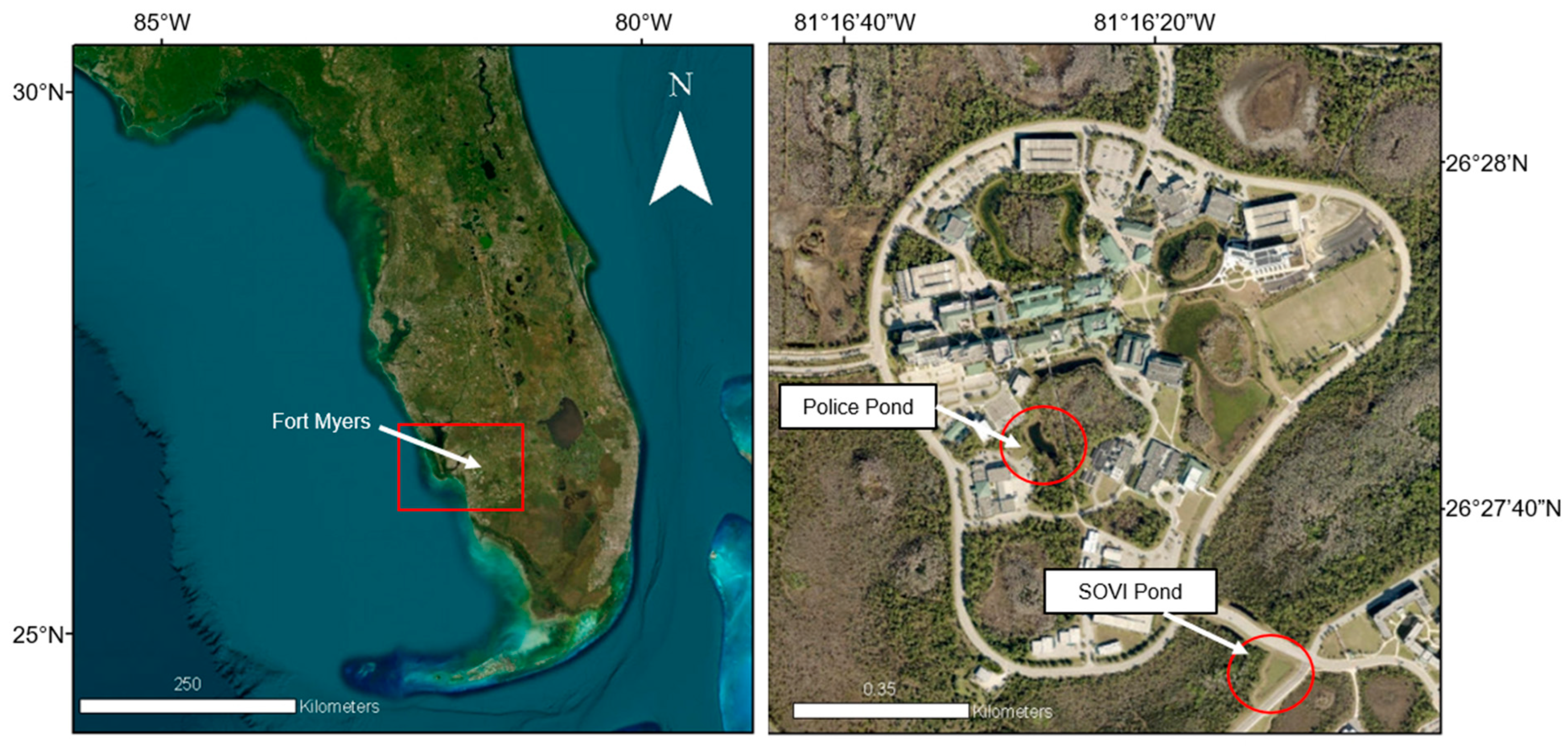
Two stormwater retention ponds on the campus of Florida Gulf Coast University were selected for investigation (Figure 1). The “SOVI Pond” (26°27′30.9″ N, 81°46′11.4″ W) is located off the southwest corner of the intersection between FGCU South Bridge Loop Road and South Village (i.e., SOVI) Boulevard, and the “Police Pond” (26°27′43.8″ N, 81°46′27.5″ W) is located east of the Campus Support Complex housing the police station. The SOVI Pond was constructed between late 2017 and late 2018, and the Police Pond was constructed in 1996. These dates were approximated based on the permitting documents from the Environmental Resource Permit (ERP) from the Florida Department of Environmental Protection and the historical imagery from Google Earth.
The SOVI and Police Pond beds consist of fine sand, sand, sandy clay loam, and fine sandy loam (USSCS 2022). Both ponds overlay a sandy limestone within the Fort Thompson Formation [25]. A shelly sand unit commonly occurs beneath the sandstone within the same formation.
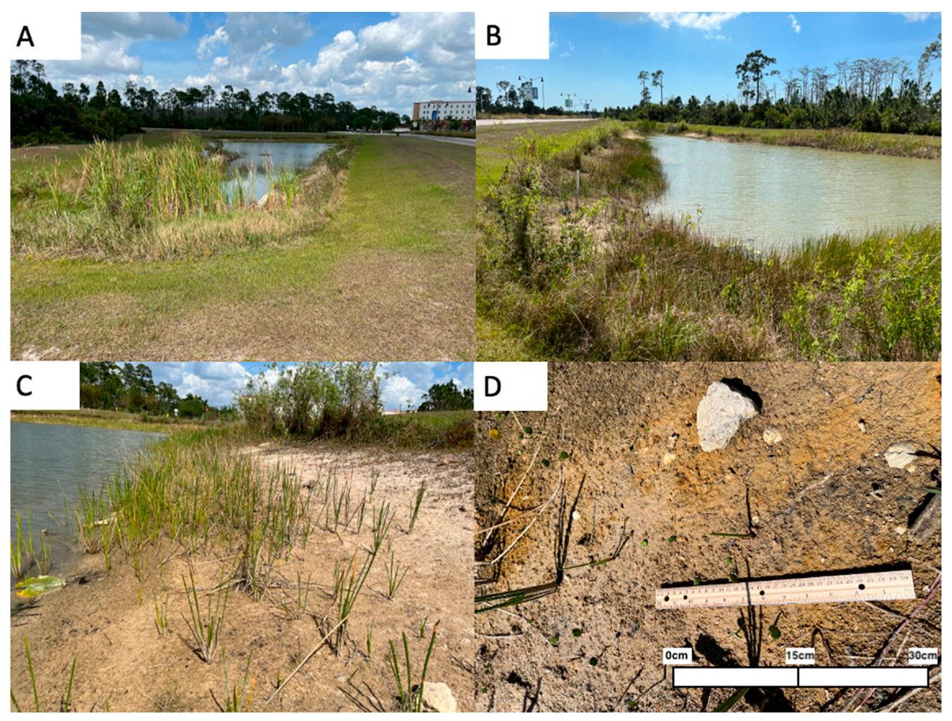
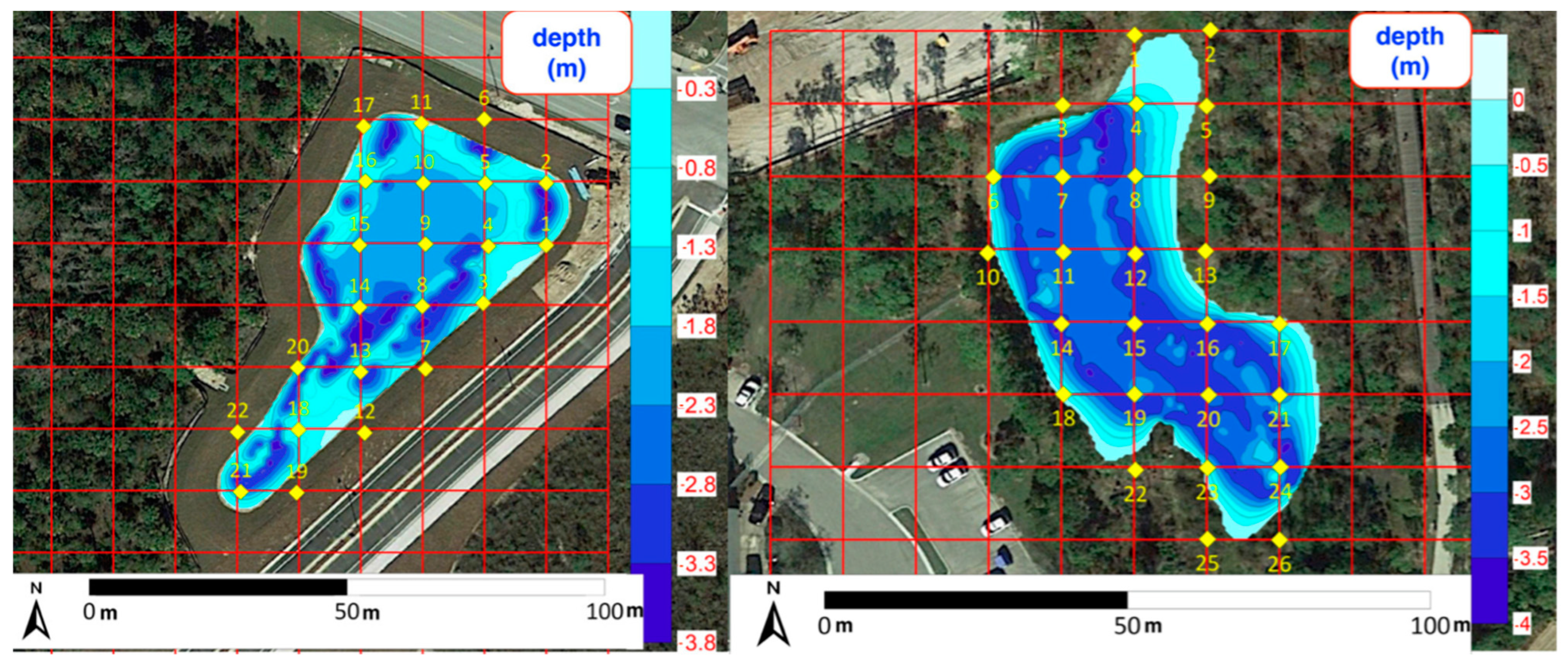
The SOVI Pond is typical of urban stormwater ponds in southern Florida (Figure 2). It contains an irregular perimeter, an interface zone containing a variety of vegetation, but predominately spikerush (Eleocharis cellulosa), some inlet pipes, and a regulated outflow structure that has a set elevation (Figure 2 and Figure 3). There is a cleared buffer area surrounding the pond with a width of about 8 m. The pond shoreline has a perimeter of about 200 m and an approximate area of 2000 m2 as its open water contracts during the dry season (31 October–1 June). At the time of the bathymetric survey, the pond had a maximum depth of about 3.8 m (Figure 3). The bathymetries of these ponds were measured using a Lowrance™ model HDS-7 Gen3 (Tulsa, OK, USA) using the integrated WAAS enhanced Global Positioning System (GPS) and a single beam 200 kHz SONAR transducer. Pond data were obtained during a moderately dry period between 20 October and 15 November 2020.
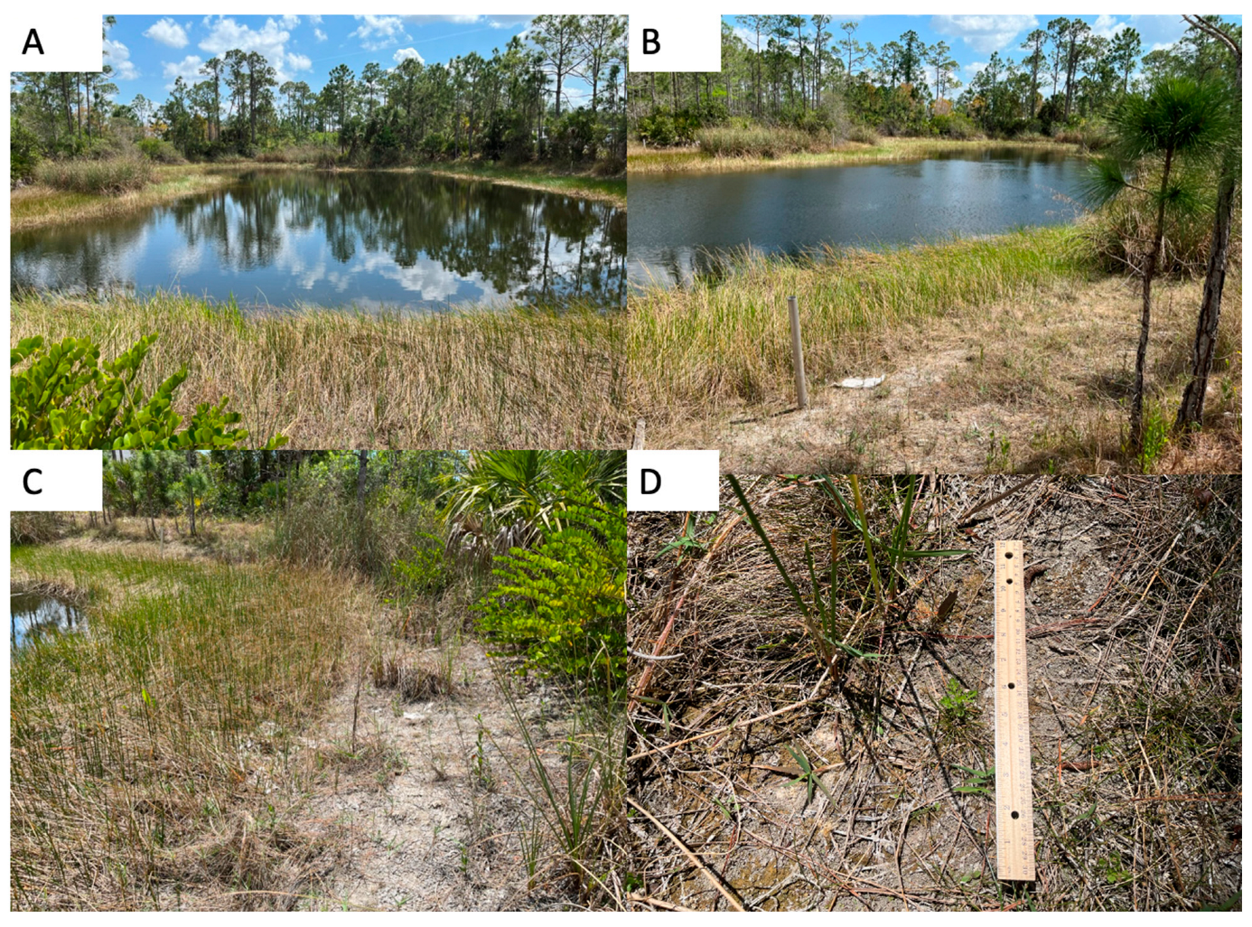
The Police Pond has a similar construction to the SOVI Pond, but does not have a vegetative buffer (Figure 4). This pond has mature vegetation close to the perimeter, which is completely covered with spikerush, a series of inflow culverts, and an overflow control structure (Figure 3 and Figure 4). The pond has a shoreline with a perimeter of 240 m and an estimated area of 2140 m2. Similar to the SOVI ponds, at the time of the bathymetric survey, the maximum water depth was about 4 m (Figure 3). The bathymetry of this pond was determined as previously described for the SOVI pond. Measurements were made between 26 November and 1 December 2020, which was a moderately dry period. Despite the dry period, dewatering from a construction project on another part of campus channeled water into the pond and maintained the water level near the control elevation.
2.2. Coring of Sediment in the Pond Bed
Coring of the sediment in the SWI of each pond bed was conducted at the numbered locations in Figure 3. These locations included peripheral sites that occurred on the edge of the water and at varying depths within the pond. Therefore, all the coring sites were fully saturated with water at the time of sampling. Further, all cores were retained in their original vertical orientation throughout the study. The cores were obtained by driving 8.9 cm (outer diameter, 0.635 cm wall thickness) clear acrylic tubes into the sediment. The minimum, maximum, mean, and median values of the sediment core lengths can be found in Supplementary Data Table S1. The tubes contained a one-way check valve at the top to allow air out during the insertion of the tube. To remove the sediment core, the valve was closed to create suction upon extraction, and the sediment core was slowly removed from the pond bed. Once removed from the pond bed, a black rubber stopper (size 14) was inserted into the bottom of the tube and then wrapped in place with electrical tape. The valve fixture at the top of the tube was then removed and replaced by an inserted rubber stopper. One core was taken per sampling station.
For deep water samples, a universal percussion corer from Aquatic Research Instruments (www.aquaticresearch.com; accessed on 1 February 2023) was used to obtain samples using a small boat for lake access. The percussion corer uses the same principle as the above-described method for removing sediment from the pond bed. Rubber stoppers and electrical tape were again used to seal the sediment cores for transport to the laboratory. Both shallow and deep water samples were stored in 19 L buckets filled with water at laboratory temperature until the hydraulic conductivity analysis could be conducted. The sample handling and preservation of shallow and deep water samples remained consistent.
2.3. Sediment Core Permeability Cell Design
The acrylic tubes, in which the cores were collected, were converted into a permeability cell to directly measure the hydraulic conductivity so that sediment layers that control vertical hydraulic conductivity would not be disturbed. The permeability cell consists of a top and bottom section (Figure 5). The top section includes a 76.2 × 50.8 mm rubber drain coupling, a 50.8 × 12.7 mm bushing, and a 12.7 × 9.525 mm on/off valve. The bottom section consists of a 7.9 cm diameter Global Gilson standard permeameter porous stone placed inside a 3D printed stone holder and a straight drain connector. The top was attached first with the valve closed, which allowed for the bottom section to be attached, with suction holding the sediment in place. Sediment tended to slide down slightly within the core pipe. Before the data collection, samples were flushed with 19 L of water as downward flow from an elevated carboy that helped to mobilize and degas biogenic-derived air bubbles from the sediment, or the samples were allowed to flush for 24 h before testing in low hydraulic conductivity samples. Downward flow in this study was utilized due to the constraints of the design. The completed permeability cell was then attached to either a falling head permeameter or a custom-made gravity drain design for samples that drained too quickly with the falling head setup, and therefore likely included a higher percentage of larger grain sizes [26,27]. The duration was measured for the falling head to pass between two separate markings on the manometer tube as in the standard method for a falling head permeameter [28]. Nine replicate measurements were taken per sediment core permeability cell sample.
The custom-made gravity drain was modified from the work of Gefell et al. [29]. This method allowed the calculation of the vertical hydraulic conductivity from sediment core drainage by measuring the time required for a given volume of water to drain from lake sediment cores (Figure 5). In the modified setup used herein, the water level was maintained as a constant head via flowing water into a carboy, with an exit valve cut into it to allow excess water to overflow (a standard constant head permeameter design). The permeability cell was configured exactly as before but sat on top of a stand with perforation for a collection funnel. A graduated cylinder was placed under the stand with a funnel, and the quantity of water collected and collection time were used to calculate the flow rate.
2.4. Grain Size Analyses
After the cell permeameter runs were completed, grain size analyses were conducted to assess to cross-check the reasonableness of the hydraulic conductivity results. Sediment cores were extruded upward and sectioned using the following visual discriminants: texture, color, and organic content (generally of very dark brown to black color). Sectioned sediments from the cores were run through a Malvern Mastersizer 3000 (www.malvernpanalytical.com; accessed on 1 February 2023) with the hydro exchangeable volume (EV) attachment to obtain grain-size distribution. Layers with a significant organic fraction (more than a few percent) could not be run through the Mastersizer. Although a layer-based approach was intended to provide the highest level of detail in the analysis, the final mean grain size used in the analysis represents an average between all layers, and the median d10 grain size was obtained from the layer that included the smallest d10 grain size, and the organic percent was obtained from the layer with the highest organic percent content. Although the d10 sizes and organic matter were calculated for all layers, selecting layers with the smallest grain size and greatest percent of organic matter were used, because these layers would represent the most hydraulically constraining layers.
2.5. Custom-Designed Falling Head Manometer for In Situ Field Usage
A second method to measure hydraulic conductivity was developed to make in situ measurements within the pond. First, a section of thin-wall aluminum tube with a 7.6 cm inner diameter was driven into the lake sediment using a fence post driver with an average depth of 40–50 cm. The tube was driven to a depth sufficient to pass through any modern sediment into the sand portion of the bottom. The exact depth was recorded as each tube was driven into the sediment. The top of the manometer was modified to contain a 3D-printed plug containing two holes. The plug was sealed using a rubber gasket and two fasteners (Figure 6). The plug was designed to contain a 10.3 mm diameter standpipe with a funnel connected at the top. The second hole in the plug was used to hold a 9.5 mm pipe. The pipes were glued into the top fitting. A ruler was glued to the back of the pipe to be able to read the water level in the field. The lower boundary was established visually before adding water to the tube. Then, the manometer was filled with water through the inlet valve to a predetermined upper boundary, and as soon as the filling ceased, the falling head test began. The test was concluded when the water level returned to the lower boundary. The falling head measurements were conducted at least three times at each site within 1 m from the core sample location.
2.6. Hydraulic Conductivity Calculations and Data Analysis
Hydraulic conductivity values were calculated for the permeability cell falling head tests and the in situ falling head tests using Equation (1), and the gravity drain constant head tests were calculated using Equation (2) following equations from ASTM D5856 [28] and Gefell et al. [29], respectively.
where h1 is head at time start, h2 is head at time stop, a (L2) is the manometer cross-sectional area, L (L) is the sediment column length, A (L2) is the sediment column cross-sectional area, and t (T) is the measurement time, and
where Q (L/T−3) is flow rate, h (L) is the hydraulic head, A (L2) is the sediment column cross-sectional area, and L (L) is soil column length.
Nine runs, and therefore nine hydraulic conductivity calculations, were made for each of the sediment cores during the laboratory tests, and three calculations were made for the in situ tests. Hydraulic conductivity values, grain sizes, and percent organic matter were statistically analyzed for both ponds and variation in depth using a one-way ANOVA test and pairwise comparison analyses in R [30].
3. Results
3.1. Hydraulic Conductivity Data Compared to Grain Size Data
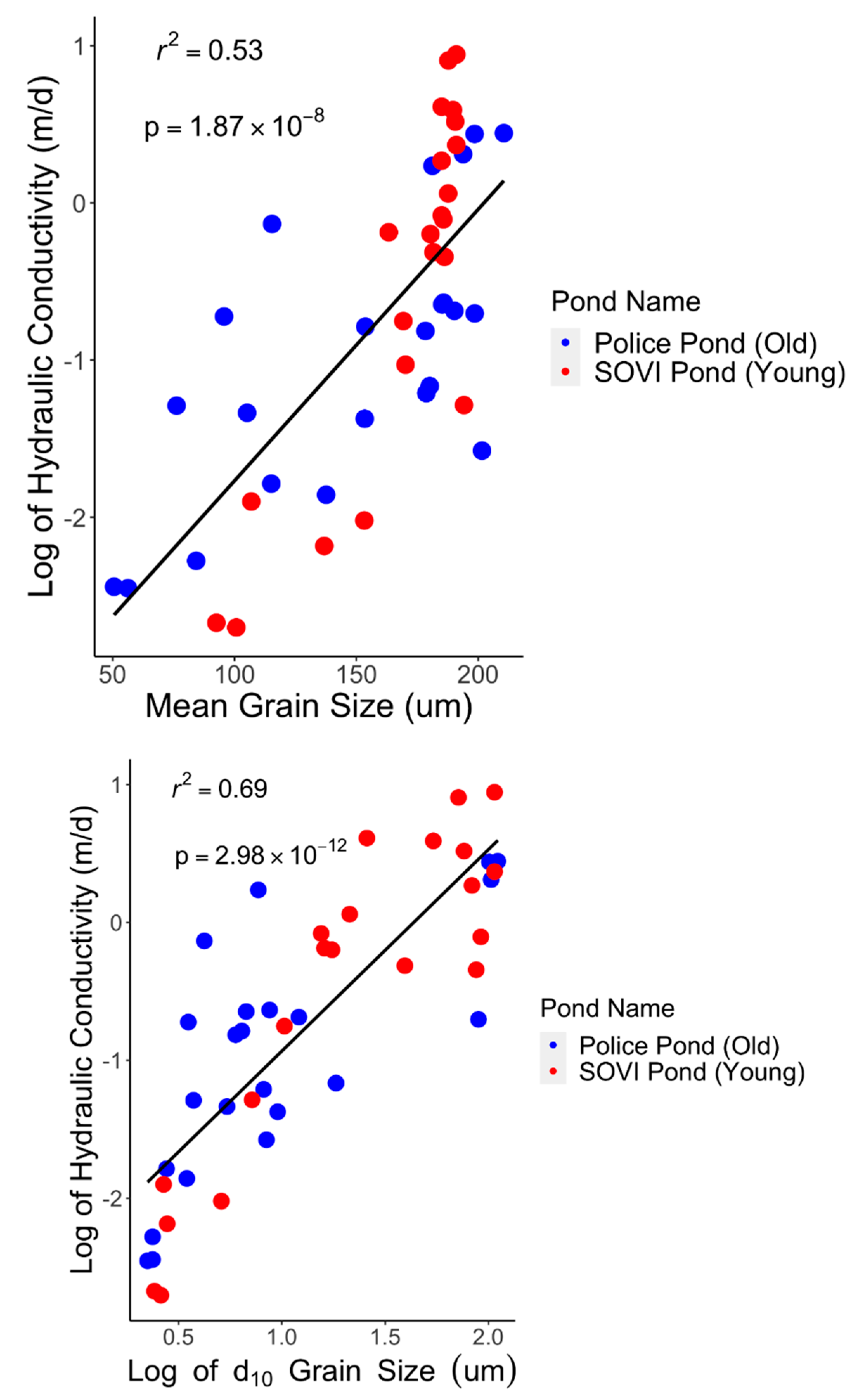
The data obtained for the hydraulic conductivity and grain size values are summarized in Supplementary Data Tables S2 and S3, respectively. A linear regression analysis was applied to the log of hydraulic conductivity values with the summed mean grain size across sediment core layers, and a second plot was made showing the relationship between the log of hydraulic conductivity and the log of the median d10 value (finest sediment) (Figure 7). While there was a strong relationship between the measured log of hydraulic conductivity and the mean grain diameter (r2 = 0.53, p = 1.87 × 10⁻⁸), the relationship between the log of hydraulic conductivity and grain size was stronger for the median d10 grain size value (r2 = 0.69, p = 2.98 × 10⁻¹²) (Figure 7). In both cases, the linear regressions were statistically significant (p < 0.05).
3.2. Field Measurement of Hydraulic Conductivity Using a Driven Aluminum Tube Standpipe and Modified Head
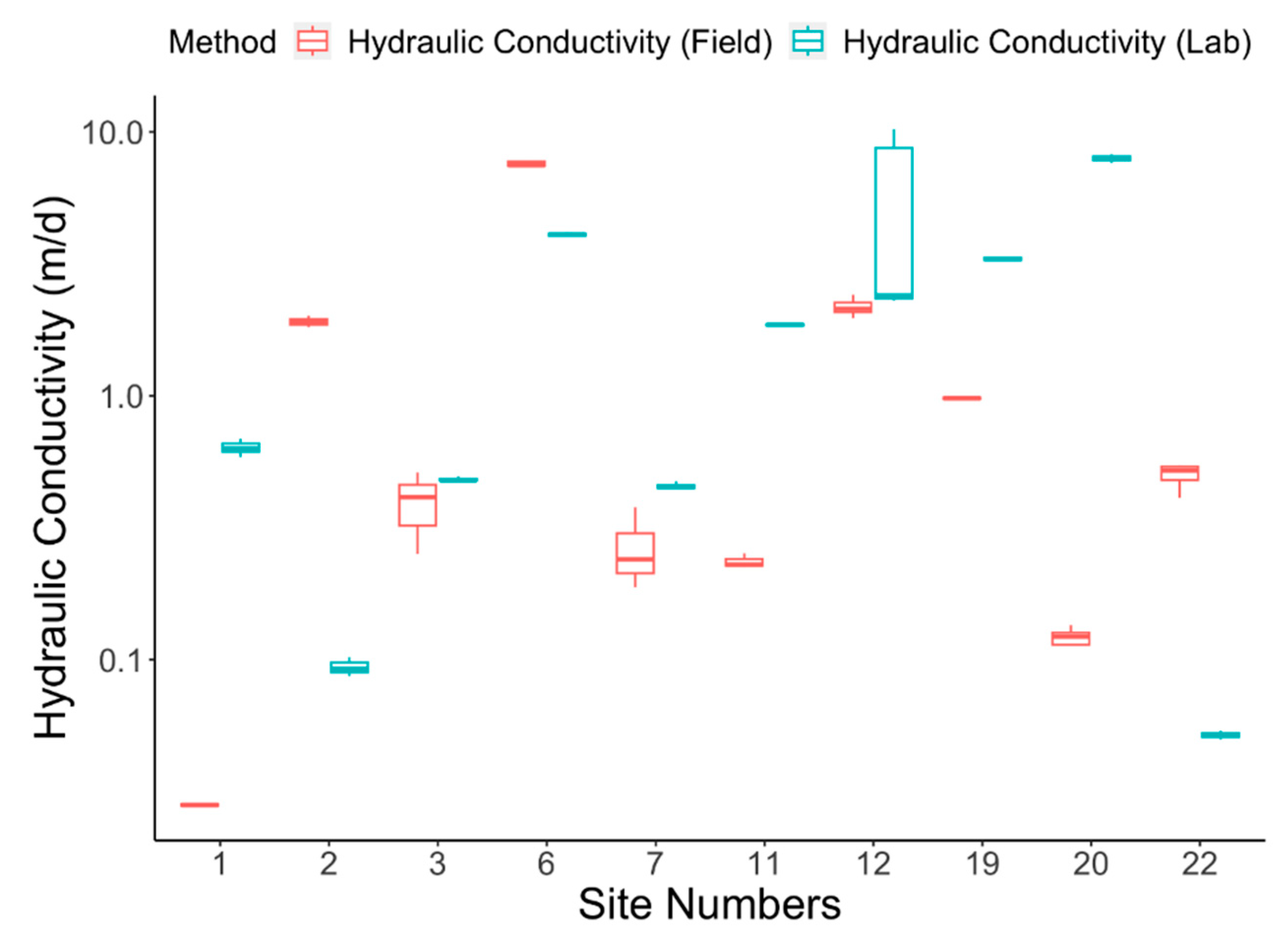
Falling head tests in the field were conducted at shallow sites that could be accessed by wading. However, only selected sites from the SOVI Pond could be measured and analyzed. Lower hydraulic conductivity sediments at the Police Pond increased water residence time in the manometer, causing thermal expansion of the water in the tube caused by intense sunlight heating of the aluminum cylinder. Gas bubbles (possibly in situ, biogenic-derived gas generation) also caused rising heads in the manometers. This issue was compounded by the choice of aluminum for the standpipe because it enhanced heating by the sun in daylight hours, and the heating likely enhanced degassing of the sediment occurring within the manometer. The degassing problem occurred wherever the sediments contained some organic material, including every site at the Police Pond.
A pairwise t-test of results found the measured hydraulic conductivity values from the laboratory and field methods were not significantly different (p = 0.31). However, significant intra-site variation occurred between the methods, as can be observed (Figure 8). Given less control of external variables in the field environment, combined with the methodological challenges previously described, a high degree of variance is to be expected. Future iterations of the manometer design should reduce intra-site variation observed in this study (e.g., use of white or clear plastic tubing instead of aluminum, or eventually conducting the measurements at night or on a cloudy day).
3.3. Grain Size and Hydraulic Conductivity Comparison between the Two Ponds
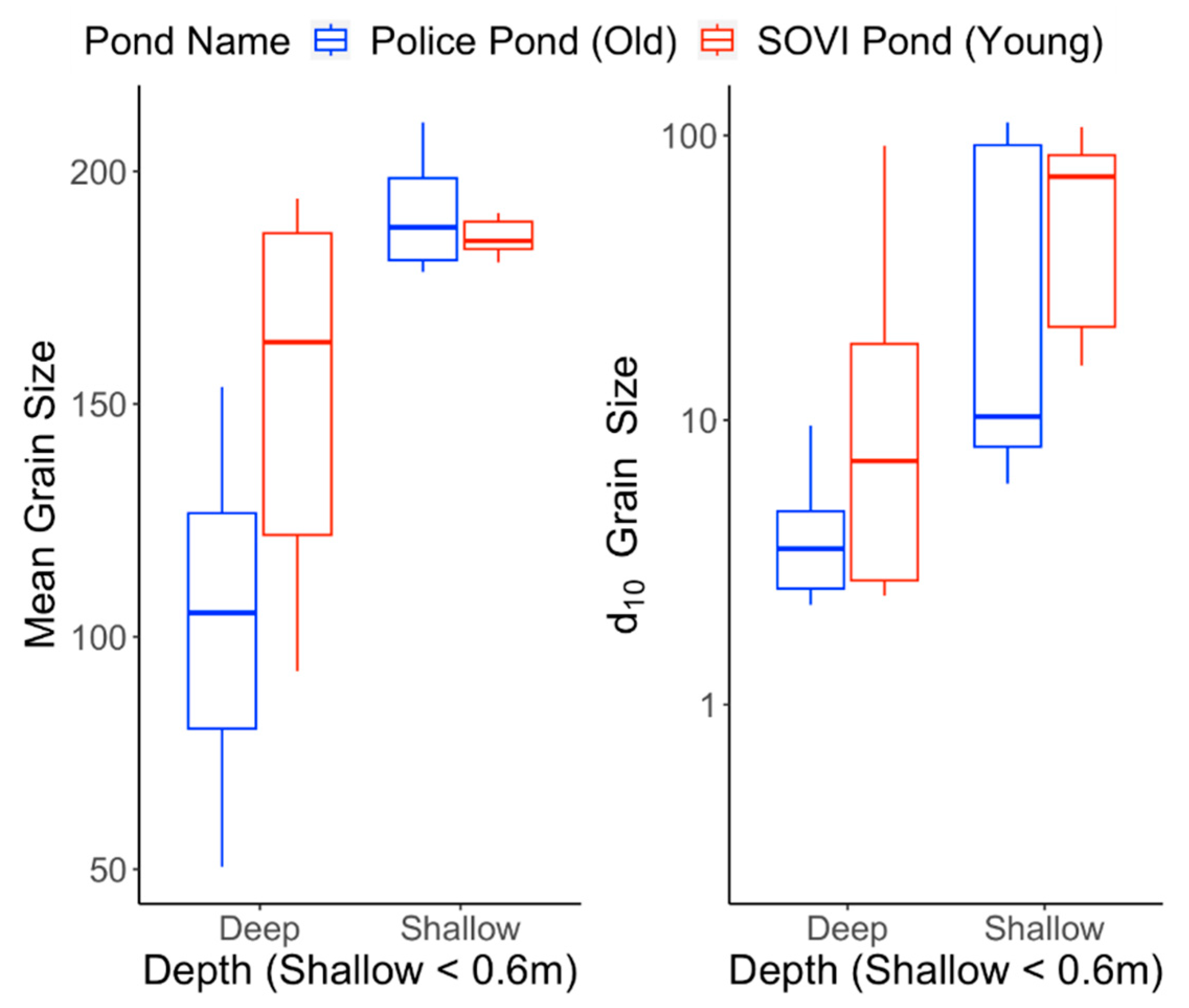
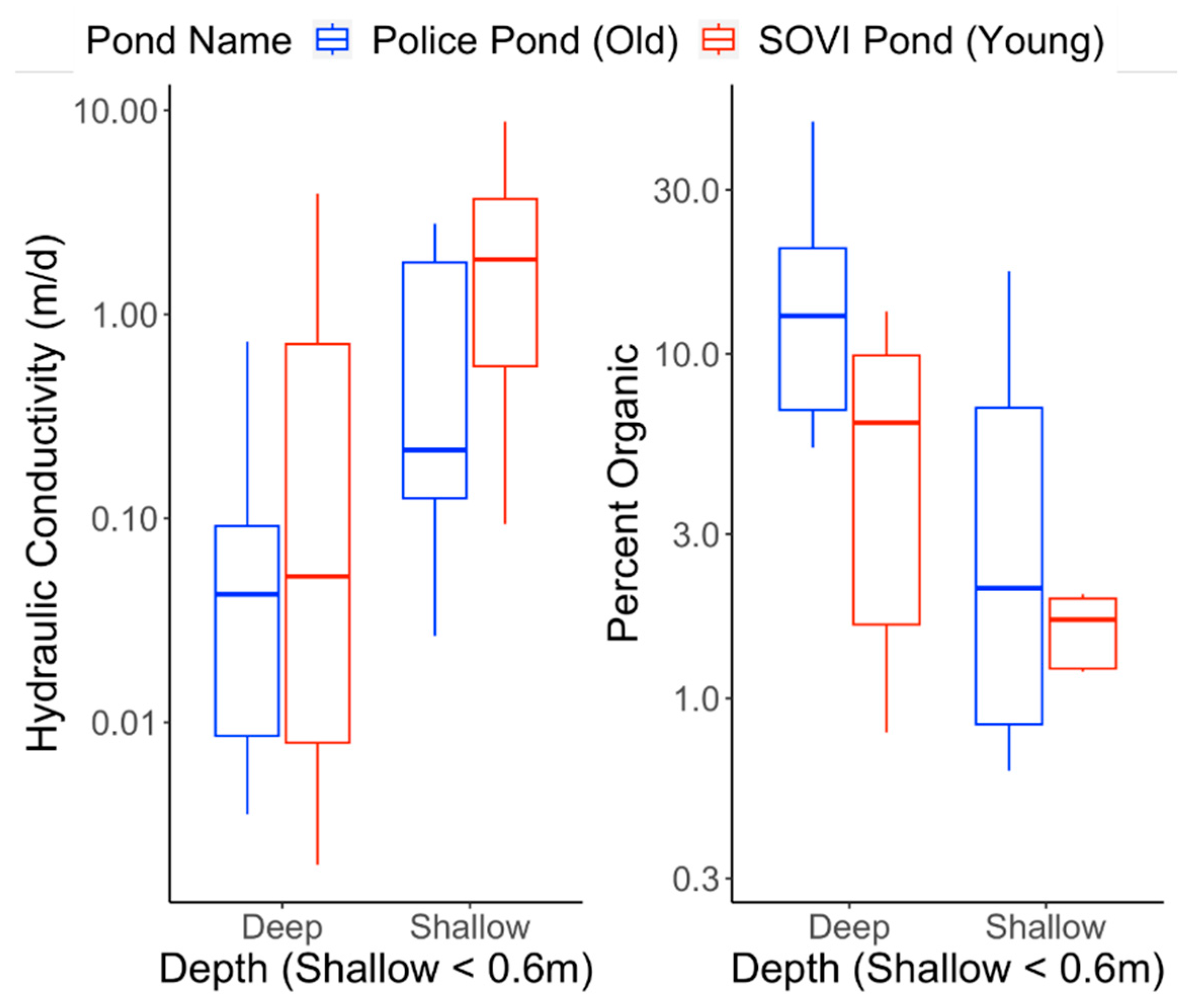
A one-way ANOVA was conducted on mean grain sizes, effective grain sizes, hydraulic conductivities, and percentages of organic matter between the Police Pond (older) and the SOVI pond (younger). Pond and depth categories as independent variables were conducted as an additive model. The mean grain size for the Police Pond (148.9 µm) was less than for the SOVI Pond (168.8 µm) and statistically significant (p = 0.0159). The median d10 grain size for the Police Pond (22.9 µm) was less than the SOVI pond (38.5 µm) and was not statistically significant (p = 0.13). The hydraulic conductivity of Police Pond (Kavg = 0.510 m/d) was less than the hydraulic conductivity of the SOVI pond (Kavg = 1.713 m/d) and was statistically significant (p = 0.025). The percentage of organic content in the Police Pond (9.9%) was higher than SOVI Pond (4.4%) and statistically significant (p = 0.027). The shallow parts of the ponds were significantly different from the deeper parts of the pond for hydraulic conductivity (p = 0.007), organic content (p = 0.0009), mean grain size (p < 0.0001), and the median d10 grain size (p = 0.0006). A comparison of these values and their respective depths (i.e., shallow, deep) is shown in Figure 9 and Figure 10.
4. Discussion
4.1. Grain Size, Hydraulic Conductivity, and Pond Age
There is a distinctive relationship between grain size distribution and the hydraulic conductivity of sediments in all depositional environments [31]. The mean grain sizes correlated (r2 = 0.53) and the median grain sizes (d10) correlated well (r2 = 0.69) with the hydraulic conductivities for the samples. This statistical correlation is similar to other studies measuring the hydraulic properties of lake beds [32]. The range in hydraulic conductivity values measured is reasonable based on the measured grain size values and medium and depositional environment [33,34]. The statistical analysis constraining for pond age (i.e., older, younger) demonstrated that the Police Pond (older) exhibited smaller mean grain sizes and smaller average hydraulic conductivities. The differences between the effective grain sizes were not statistically significant and may be influenced by the wider range of grain sizes in the deeper depths of the younger pond. Additionally, the hydraulic conductivities of the older pond were smaller, which aligns with both the smaller average and effective grain sizes in both shallow and deeper depths. The percentage of organic matter was much higher in the older pond, indicating that the hydraulic conductivity of the sediment likely decreases over time in stormwater retention ponds and, therefore, limits recharge to the shallow aquifer. A buildup of low permeability layers is a natural process in lacustrine systems [35,36]. However, the detection of reductions in hydraulic conductivity observed here indicates that stormwater pond performance is reduced in a geologically short period. The sample size was not sufficient for examining differences within depth categories.
Among the clay and silt fractions of the sediment, there was an organic component, which could not be measured in the laboratory. High-temperature removal of the organic fraction (greater than a few percent) was inappropriate because it would potentially also remove the carbonate fraction of the silt and clay and could aggregate fine particles into large grain size fractions. However, the observed decrease in the median d10 grain size and increase in organic content for the shallow parts of the older pond indicate a build-up of silt and organic matter that could reduce hydraulic conductivity. This is particularly important for the SWI on the nearshore margins where the SWI flux is higher due to a higher sloping groundwater surface [5], but may also be considered at depth during dry conditions when the groundwater surface occurs beneath the pond bottom [37]. Future research should continue to investigate how hydraulic conductivity changes as ponds age, and how the reduction impacts the desired functions.
4.2. Advantages and Disadvantages of Custom Permeability Cell
Hydraulic conductivity testing via the custom permeability cell allowed for hydraulic conductivity measurements of the cores with minimal disturbance to sediment layering. In particular, very thin surficial layers (such as silt, clay, and biofilms) were measured. Measuring hydraulic conductivity from sediment cores has an advantage in deep water, where the installation of seepage meters, when used on rare occasions for this purpose, is difficult and may still require the installation of piezometers if measuring hydraulic conductivity. The sediment core to permeability cell method also has the advantage of obtaining geologic information, as the sediment cores can be examined after the hydraulic conductivity testing is completed. It is, however, cumbersome and difficult to transport sediment cores to the laboratory, as well as maintain a vertical orientation so that the sediment is not disturbed. Further, the flushing protocol is time-consuming and the degassing of biogenic-derived air bubbles may not be needed due to their effect on accurate hydraulic conductivity values, in addition to purging air bubbles with a more traditional upward flow.
A few additional methodological concerns should be considered for future research. Gas bubbles tend to get trapped in the falling head manometer and obstruct the test. However, in situ gas bubbles can also impede flow, and removing them could inflate hydraulic conductivity values. Perhaps one approach to the gas release is to allow the in situ permeability cell to rest between one week and one month, during which the gas could vent into the atmosphere. The “rest” model would likely cause less perturbation to the sediment properties than agitating the installed pipe. Another possible method to alleviate the degassing issue is the use of larger diameter tubing. For the falling head manometer setup, the larger diameter tube would potentially negate the need to remove the bubbles. This would save time and may be more methodologically sound. More research should be conducted on comparing the gravity drain method and the falling head method. The high variance (2.34–8 m/d) shown for the lab results at site 12 (Figure 8) was due to this particular core being measured by the gravity drain and falling head methods. The hydraulic conductivity of this core was likely at the lower boundary of what the gravity drain method could reliably measure. Based on the manometer setup used, the hydraulic conductivity measurements were at the upper boundary or human error could have been a factor.
4.3. Advantages and Disadvantages of In Situ Falling Head Manometer Design
The manometer design presented here came from the need to rapidly measure head drops in a standpipe. The first issue, the thermal conductivity of the aluminum standpipe, caused heating and expansion of the water in the tube. Perhaps using clear or white PVC pipe or performing the measurements during cooler temperatures, such as on cloudy days or at night, would improve measurements. The second issue, wherein gas was released from organic-rich sediment during attempted measurements, may be resolved with future design iterations including a venting system. Another issue that was not quantified was the compression of the sediment occurring during the installation process, which potentially caused lower hydraulic conductivity values in these samples.
The in situ falling head measurement also shares some of the same advantages and disadvantages of the sediment core to the permeability cell approach. The standpipe does not puncture the top part of the interface, leaving these surficial layers that would be punctured by a piezometer intact. The standpipe is a point measurement, but more point measurements should be possible over the sediment core permeability cell or the seepage meter–piezometer approach. If the sediment is extracted as a sediment core, these time savings could be negated. More of the sediment is potentially disturbed by friction from the standpipe wall during insertion and sediment extrusion. Similar to sediment coring, low hydraulic conductivity across the SWI may be missed by not inserting the standpipe deep enough. However, unlike laboratory testing, such layers may affect the in situ hydraulic conductivity measurement [38].
4.4. Evolution of Stormwater Ponds in Time
Stormwater ponds are expected to evolve in time with changes in the bottom hydraulic conductivity. Indeed, they are used to gather urban runoff that is high in suspended solids, nutrients, and organic carbon. Compared to natural lakes, stormwater ponds are subject to accelerated changes (“aging”) due to their design. This includes the storage of surplus water, including groundwater from dewatering activities, which can bring a large amount of turbidity, including nutrients and heavy metals, into these low-flowing waters at high, or unnatural, rates and residence times [18,39,40]. Geological and biological processes play an important role in the evolution of stormwater ponds, which require pond monitoring to maintain their efficacy. Enhanced nutrient concentrations can lead to the formation of thin biofilms in the shallow saturated areas of the pond perimeter. These films can be nearly impervious. Based on the influx of urban runoff and fine-grained suspended solids, the bottom sediment is expected to become finer with time. The ponds must function not only to manage runoff during the wet season but also to support shallow water ecological systems that are important in treating nutrient-laden water. More research is needed to learn how to better manage stormwater pond effectiveness as it changes over time and when excavation or perimeter maintenance is required to maintain their recharge function.
5. Conclusions
Despite the difficulties associated with measuring the hydraulic conductivity across the SWI within stormwater retention ponds, this study effectively measured the parameter in two stormwater ponds having an age difference of 22 years. These methods allowed laboratory and in situ hydraulic conductivity measurements to be made without disturbing fine laying with the sediments of the substrate, as well as provided for detailed grain size and organic matter analyses. Results presented in this study demonstrate that sediment grain size in stormwater ponds is correlated to time and depth, reducing hydraulic conductivity, limiting recharge, and degrading the effectiveness of the stormwater control structure. The younger pond did have a statistically significant higher average hydraulic conductivity compared to the older pond.
The use of in situ direct measurement of the hydraulic conductivity across the SWI was explored using a field permeameter created from a thin-walled pipe driven into the sediment across the SWI and adding water to the top to make falling head measurements. While this method was not always successful, due to heating of the water inside the device and gas release, the method should be refined for greater use because it can be effective to make numerous measurements within a relatively short timeframe. New measurement methods need to be developed to allow a greater number of actual hydraulic conductivity measurements to be made across the SWI, especially to calibrate advanced geophysical methods that could be used to create a more effective spatial coverage of the lake bottom.
It is quite important to understand the changes in stormwater pond bottom sediments with time, because as new fine-grained material and organics are deposited, the groundwater recharge function of the ponds is reduced. The primary purposes of necessitating the construction of stormwater ponds is to provide compensatory storage to the groundwater system to mitigate the impacts of impervious surfaces associated with development and to slow water movement to discharge points to treat water quality. The loss of the groundwater recharge function exacerbates stormwater runoff, therefore reducing groundwater levels and facilitating downstream flooding. Periodic measurement of the bottom sediment hydraulic conductivity is necessary to determine when maintenance needs to be conducted to remove sediments that inhibit the recharge function.
Supplementary Materials
The following supporting information can be downloaded at: https://www.mdpi.com/article/10.3390/w15061122/s1. The Supplementary Materials show all of the actual measurements made during the research.
Author Contributions
D.C.C. did the field and laboratory work and wrote the first text draft. S.T. directed the project and rewrote parts of the text. R.R.R. provided technical advice and worked on the figures and text. T.M.M. funded the project, provided advice on the field and laboratory work, and worked on the final text. All authors have read and agreed to the published version of the manuscript.
Funding
Funding was obtained by T.M.M under the Eminent Scholar Program provided to him by the State of Florida (no grant number).
Data Availability Statement
All of the data collected are contained in the text of the paper or the Supplemental Materials.
Acknowledgments
The authors wish to thank the Emergent Technologies Institute and Christian Bokrand and Michael Hegy (3D printing) for use of the facilities to construct the laboratory permeameters and the field standpipe apparatus.
Conflicts of Interest
The authors declare no conflict of interest.
References
- Rosenberry, D.O.; LaBaugh, J.W. Field Techniques for Estimating Water Fluxes between Surface Water and Groundwater. In U.S. Geological Survey Techniques and Methods 4-D2; U.S. Geological Survey: Reston, VA, USA, 2008. [Google Scholar]
- Rosenberry, D.O.; Toran, L.; Nyquist, J.E. Effect of surficial disturbance on exchange between groundwater and surface water in nearshore margins. Water Resour. Res. 2010, 46, W06518. [Google Scholar] [CrossRef]
- Karan, S.; Kidmose, J.; Engesgaard, P.; Nilsson, B.; Frandsen, M.; Ommen, D.A.O.; Flindt, M.R.; Andersen, F.Ø.; Pedersen, O. Role of a groundwater–lake interface in controlling seepage of water and nitrate. J. Hydrol. 2014, 517, 791–802. [Google Scholar] [CrossRef]
- Baveye, P.; Vandevivere, P.; Hoyle, B.L.; DeLeo, P.C.; de Lozada, D.S. Environmental impact and mechanisms of the biological clogging of saturated soils and aquifer materials. Crit. Rev. Environ. Sci. Technol. 1998, 28, 123–191. [Google Scholar] [CrossRef] [Green Version]
- McBride, M.S.; Pfannkuch, H.O. The distribution of seepage within lakebeds. J. Res. U.S. Geol. Surv. 1975, 3, 505–512. [Google Scholar]
- Kalbus, E.; Reinstorf, F.; Schirmer, M. Measuring methods for groundwater-surface water interactions: A review. Hydrol. Earth Syst. Sci. 2006, 10, 873–887. [Google Scholar] [CrossRef] [Green Version]
- Rosenberry, D.O.; Lewandowski, J.; Meinikmann, K.; Nützmann, G. Groundwater—The disregarded component in lake water and nutrient budgets. Part 1: Effects of groundwater on hydrology. Hydrol. Process. 2015, 29, 2895–2921. [Google Scholar] [CrossRef]
- Roy, A.H.; Wenger, S.J.; Fletcher, T.D.; Walsh, C.J.; Ladson, A.R.; Shuster, W.D.; Thurston, H.W.; Brown, R.R. Impediments and solutions to sustainable, watershed-scale urban stormwater management: Lessons from Australia and the United States. Environ. Manag. 2008, 42, 344–359. [Google Scholar] [CrossRef]
- Edgar, W.W.; Maršálek, J. Comprehensive stormwater pond monitoring. Water Sci. Technol. 1994, 29, 337–345. [Google Scholar] [CrossRef]
- Rosenberry, D.O.; Duque, C.; Lee, D.R. History and evolution of seepage meters for quantifying flow between groundwater and surface water: Part 1—Freshwater settings. Earth-Sci. Rev. 2020, 204, 103167. [Google Scholar] [CrossRef]
- Lee, D.R.; Cherry, J.A. A field exercise on groundwater flow using seepage meters and mini-piezometers. J. Geol. Educ. 1979, 27, 6–10. [Google Scholar] [CrossRef]
- Chen, X. Measurement of streambed hydraulic conductivity and its anisotropy. Environ. Geol. 2000, 39, 1317–1324. [Google Scholar] [CrossRef]
- Landon, M.K.; Rus, D.L.; Edwin Harvey, F.E. Comparison of instream methods for measuring hydraulic conductivity in sandy streambeds. Groundwater 2001, 39, 870–885. [Google Scholar] [CrossRef] [Green Version]
- Baxter, C.; Hauer, F.; Woessner, W. Measuring groundwater–stream water exchange: New techniques for installing minipiezometers and estimating hydraulic conductivity. Trans. Am. Fish. Soc. 2003, 132, 493–502. [Google Scholar] [CrossRef]
- Seeberg-Elverfeldt, J.; Schlüter, M.; Feseker, T.; Kölling, M. Rhizon sampling of porewaters near the sediment-water interface of aquatic systems. Limnol. Oceanogr. Methods 2005, 3, 361–371. [Google Scholar] [CrossRef]
- Robinson, M.; Gallagher, D.; Reay, W. Field observations of tidal and seasonal variations in ground water discharge to tidal estuarine surface water. Groundw. Monit. Remediat. 1998, 18, 83–92. [Google Scholar] [CrossRef]
- Vaasma, T. Grain-size analysis of lacustrine sediments: A comparison of pre-treatment methods. Est. J. Ecol. 2008, 57, 231–243. [Google Scholar] [CrossRef] [Green Version]
- Erickson, A.J.; Taguchi, V.J.; Gulliver, J.S. The challenge of maintaining stormwater control measures: A synthesis of recent research and practitioner experience. Sustainability 2018, 10, 3666. [Google Scholar] [CrossRef] [Green Version]
- Constantz, J. Heat as a tracer to determine streambed water exchanges. Water Resour. Res. 2008, 44, W00D10. [Google Scholar] [CrossRef]
- Selker, J.S.; Thévenaz, L.; Huwald, H.; Mallet, A.; Luxemburg, W.; van de Giesen, N.; Stejskal, M.; Zeman, J.; Westhoff, M.; Parlange, M.B. Distributed fiber-optic temperature sensing for hydrologic systems. Water Resour. Res. 2006, 42, W12202. [Google Scholar] [CrossRef] [Green Version]
- Tyler, S.W.; Selker, J.S.; Hausner, M.B.; Hatch, C.E.; Torgersen, T.; Thodal, C.E.; Schladow, S.G. Environmental temperature sensing using Raman spectra DTS fiber-optic methods. Water Resour. Res. 2009, 45, W00D23. [Google Scholar] [CrossRef] [Green Version]
- Blume, T.; Krause, S.; Meinikmann, K.; Lewandowski, J. Upscaling lacustrine groundwater discharge rates by fiber-optic distributed temperature sensing. Water Resour. Res. 2013, 49, 7929–7944. [Google Scholar] [CrossRef] [Green Version]
- Binley, A.; Ullah, S.; Heathwaite, A.L.; Heppell, C.; Byrne, P.; Lansdown, K.; Trimmer, M.; Zhang, H. Revealing the spatial variability of water fluxes at the groundwater-surface water interface. Water Resour. Res. 2013, 49, 3978–3992. [Google Scholar] [CrossRef]
- Binley, A.; Hubbard, S.S.; Huisman, J.A.; Revil, A.; Robinson, D.A.; Singha, K.; Slater, L.D. The emergence of hydrogeophysics for improved understanding of subsurface processes over multiple scales. Water Resour. Res. 2015, 51, 3837–3866. [Google Scholar] [CrossRef] [PubMed] [Green Version]
- Missimer, T. The geology of South Florida: A summary. In Environments of South Florida, Present and Past II; Gleason, P.J., Ed.; Miami Geological Society: Coral Gables, FL, USA, 1984; pp. 385–404. [Google Scholar]
- Nagy, L.; Tabácks, A.; Huszák, T.; Mahler, A.; Varga, G. Comparison of permeability testing methods. In Proceedings of the 18th International Conference on Soil Mechanics and Geotechnical Engineering, Paris, France, 2–6 September 2013; pp. 399–402. [Google Scholar]
- Wilson, M.A.; Hoff, W.D.; Brown, R.J.E.; Carter, M.A. A falling head permeameter for the measurement of the hydraulic conductivity of granular solids. Rev. Sci. Instrum. 2000, 71, 3942–3946. [Google Scholar] [CrossRef]
- Standard D5856; Test Method for Measurement of Hydraulic Conductivity of Porous Material Using a Rigid-Wall, Compaction-Mold Permeameter. American Standard for Testing and Materials (ASTM) International: West Conshohocken, PA, USA, 2015. [CrossRef]
- Gefell, M.J.; Larue, M.; Russell, M.K. Vertical hydraulic conductivity measurement by gravity drainage. Groundwater 2019, 57, 511–516. [Google Scholar] [CrossRef] [PubMed]
- R Core Team. R: A Language and Environment for Statistical Computing; R Foundation for Statistical Computing: Vienna, Austria, 2013. [Google Scholar]
- Rosas, J.; Lopez, O.; Missimer, T.M.; Coulibaly, K.M.; Dehwah, A.H.A.; Sesler, K.; Lujan, L.R.; Mantilla, D. Determination of hydraulic conductivity from grain-size distribution for different depositional environments. Groundwater 2014, 52, 399–413. [Google Scholar] [CrossRef]
- Tecklenburg, C.; Blume, T. Identifying, characterizing and predicting spatial patterns of lacustrine groundwater discharge. Hydrol. Earth Syst. Sci. 2017, 21, 5043–5063. [Google Scholar] [CrossRef] [Green Version]
- Deshesne, M.; Barraud, S.; Bardin, J.-P. Indicators for hydraulic and pollution retention assessment of stormwater infiltration basins. J. Environ. Manag. 2004, 71, 371–380. [Google Scholar] [CrossRef]
- Belkhatir, M.; Schanz, T.; Arab, A.; Della, N.; Kadri, A. Insight into the effects of gradation on the pore pressure generation of sand–silt mixtures. Geotech. Test. J. 2014, 37, 922–931. [Google Scholar] [CrossRef]
- Likens, G.E.; Davis, M.B. Post-glacial history of Mirror Lake and its watershed in New Hampshire, USA: An initial report. Int. Ver. Für Theor. Und Angew. Limnol. Verh. 1975, 19, 982–993. [Google Scholar]
- Wetzel, R.G. Role of the littoral zone and detritus in lake metabolism. Arch. Hydrobiol. 1979, 13, 145–161. [Google Scholar]
- Chen, X. Hydrologic connections of a stream–aquifer-vegetation zone in south-central Platte River valley, Nebraska. J. Hydrol. 2007, 333, 554–568. [Google Scholar] [CrossRef]
- Burnette, M.C.; Genereux, D.P.; Birgand, F. In-situ falling-head test for hydraulic conductivity: Evaluation in layered sediments of an analysis derived for homogenous sediments. J. Hydrol. 2016, 539, 319–329. [Google Scholar] [CrossRef] [Green Version]
- Lawrence, A.I.; Marsalek, J.; Ellis, J.B.; Urbonas, B. Stormwater detention & BMPs. J. Hydraul. Res. 1996, 34, 799–813. [Google Scholar]
- Walker, D.J. Modelling residence time in stormwater ponds. Ecol. Eng. 1998, 10, 247–262. [Google Scholar] [CrossRef]
Figure 1.
Location map showing the location of Fort Myers, Florida (left) and the stormwater pond locations on the campus of Florida Gulf Coast University (right).
Figure 1.
Location map showing the location of Fort Myers, Florida (left) and the stormwater pond locations on the campus of Florida Gulf Coast University (right).

Figure 2.
Pictures of the SOVI Pond taken during the dry season: (A) view of the lake facing north showing vegetative growth near inlets and control structures. (B) View of the pond facing south showing areas of heavily and poorly vegetated shoreline. (C) View of the shoreline facing north showing the natural soil and colonizing spikerush (Eleocharis cellulosa). (D) Close-up view of the soil showing young spikerush shoots.

Figure 3.
Depth variation and core locations in the SOVI (left) and Police (right) Ponds. Locations are approximate. Samples sites shown near the pond edges were taken in the pond in fully saturated conditions. Certain sites (such as 1 and 23) were rocky and could not be sampled.
Figure 3.
Depth variation and core locations in the SOVI (left) and Police (right) Ponds. Locations are approximate. Samples sites shown near the pond edges were taken in the pond in fully saturated conditions. Certain sites (such as 1 and 23) were rocky and could not be sampled.

Figure 4.
Pictures of the Police Pond taken in the dry season. (A) View facing south showing the heavily vegetated shoreline colonized completely by spikerush. (B) View facing east shows more of the heavily vegetated shoreline with some exposed shoreline. (C) View along a section of shoreline showing some unvegetated patches alternating with spikerush patches. (D) Close-up view of exposed soil patch showing some spikerush and other vegetation, as well as detritus covering. Algal mats were also present.

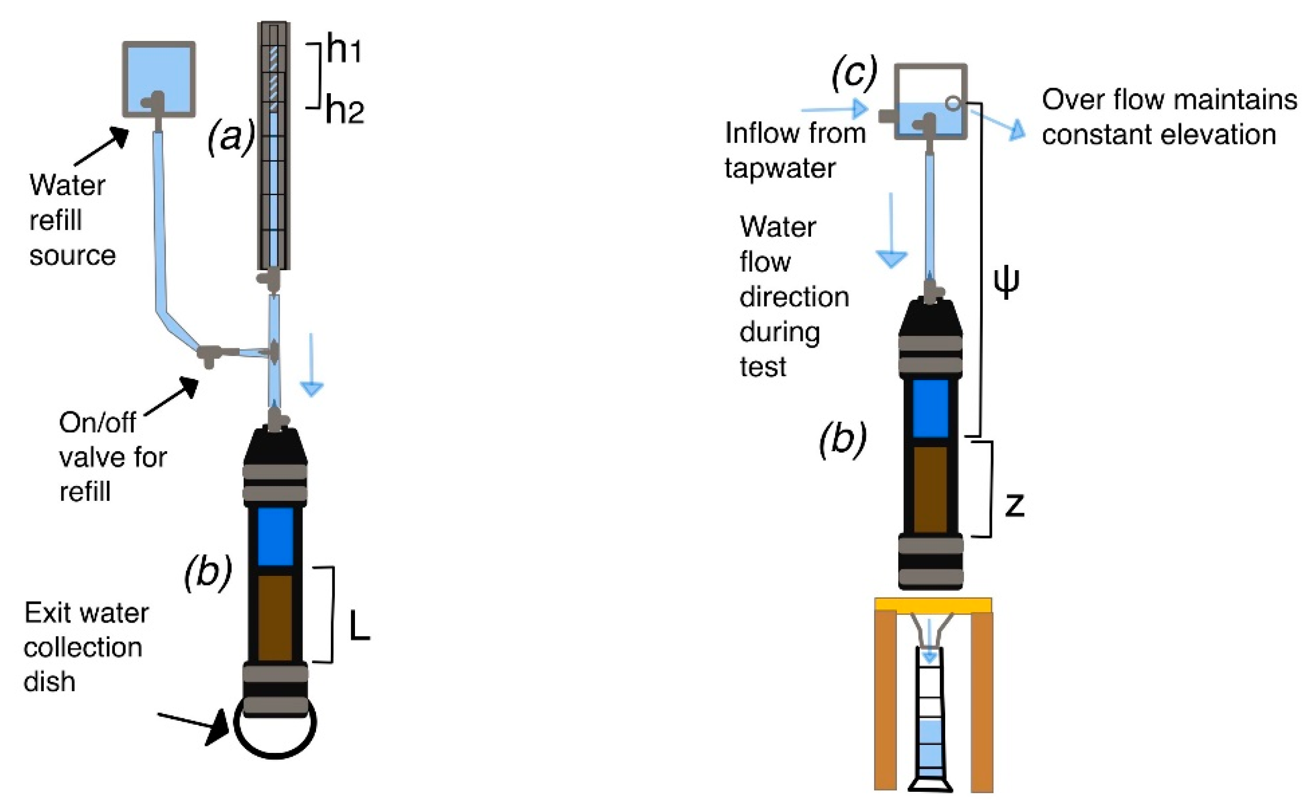
Figure 5.
Permeability cell setup. (a) Falling head manometer attached to the (b) permeability cell (blue = water, brown = sediment) and carboy with an on/off valve used to refill the manometer and an overflow dish at the base. The gravity drain design (c) attached the (b) permeability cell. The black and grey caps on the top and bottom of the permeability cells are rubber drain couplings with metal clasps.

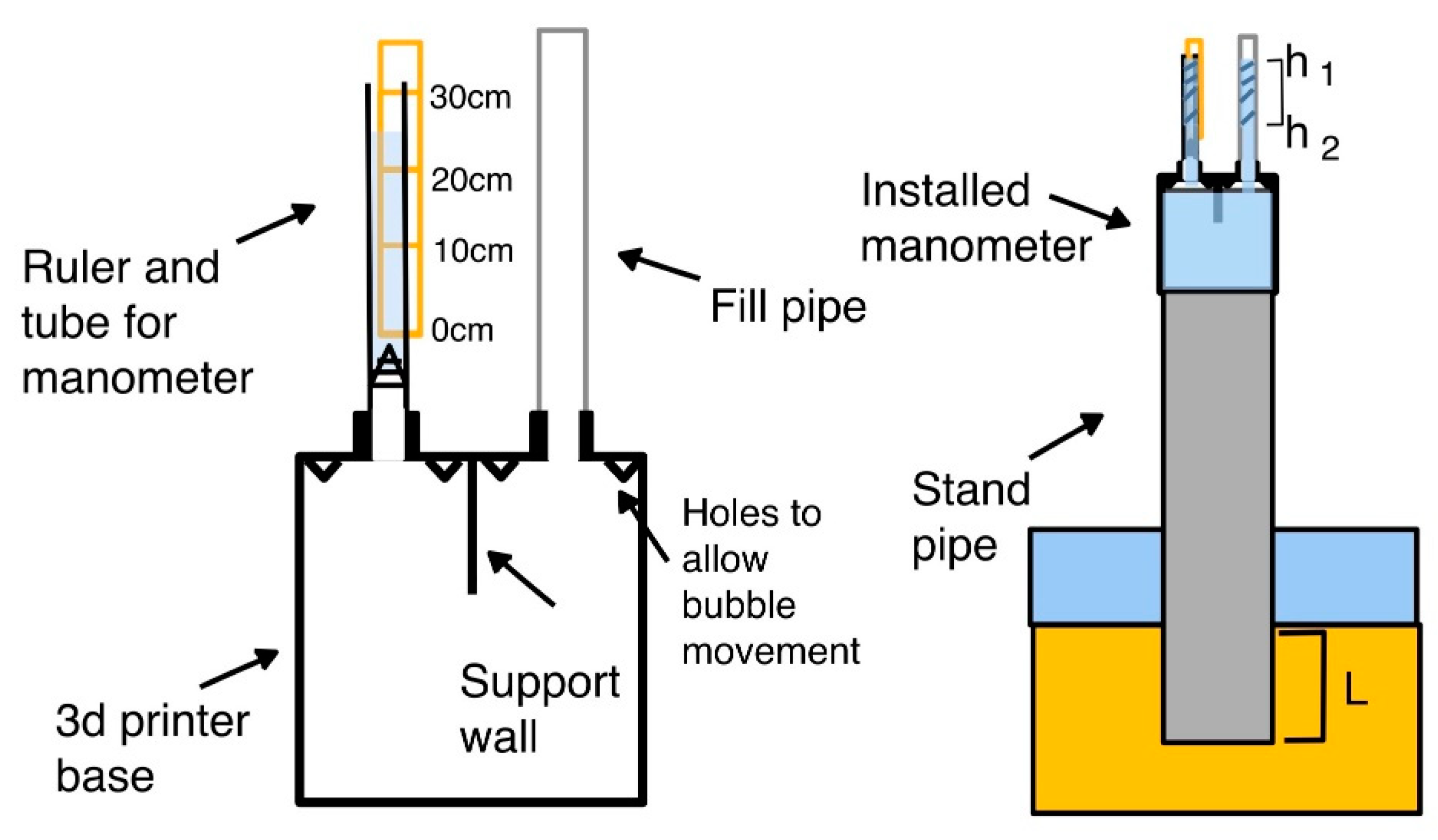
Figure 6.
In situ standing head manometer setup deployed in the SOVI Pond.

Figure 7.
Measurements of the log of hydraulic conductivity with the mean grain diameter of the bottom sediment (top) and measured log of hydraulic conductivity with the log of the median d10 grain size value (bottom).
Figure 7.
Measurements of the log of hydraulic conductivity with the mean grain diameter of the bottom sediment (top) and measured log of hydraulic conductivity with the log of the median d10 grain size value (bottom).

Figure 8.
Comparison of laboratory-measured hydraulic conductivity and the field manometer method.

Figure 9.
Grain size comparison between the Police Pond constructed in 1996 and the SOVI Pond constructed in 2017.
Figure 9.
Grain size comparison between the Police Pond constructed in 1996 and the SOVI Pond constructed in 2017.

Figure 10.
Hydraulic conductivity comparison and organic material between Police Pond constructed in 1996 and SOVI Pond constructed in 2017.
Figure 10.
Hydraulic conductivity comparison and organic material between Police Pond constructed in 1996 and SOVI Pond constructed in 2017.

Disclaimer/Publisher’s Note: The statements, opinions and data contained in all publications are solely those of the individual author(s) and contributor(s) and not of MDPI and/or the editor(s). MDPI and/or the editor(s) disclaim responsibility for any injury to people or property resulting from any ideas, methods, instructions or products referred to in the content. |
© 2023 by the authors. Licensee MDPI, Basel, Switzerland. This article is an open access article distributed under the terms and conditions of the Creative Commons Attribution (CC BY) license (https://creativecommons.org/licenses/by/4.0/).
Share and Cite
MDPI and ACS Style
Canfield, D.C.; Thomas, S.; Rotz, R.R.; Missimer, T.M. Stormwater Pond Evolution and Challenges in Measuring the Hydraulic Conductivity of Pond Sediments. Water 2023, 15, 1122. https://doi.org/10.3390/w15061122
AMA Style
Canfield DC, Thomas S, Rotz RR, Missimer TM. Stormwater Pond Evolution and Challenges in Measuring the Hydraulic Conductivity of Pond Sediments. Water. 2023; 15(6):1122. https://doi.org/10.3390/w15061122
Chicago/Turabian StyleCanfield, Daniel C., Serge Thomas, Rachel R. Rotz, and Thomas M. Missimer. 2023. "Stormwater Pond Evolution and Challenges in Measuring the Hydraulic Conductivity of Pond Sediments" Water 15, no. 6: 1122. https://doi.org/10.3390/w15061122
Note that from the first issue of 2016, this journal uses article numbers instead of page numbers. See further details here.