Online Control of the Raw Water System of a High-Sediment River Based on Deep Reinforcement Learning

Abstract

Water supply systems that use rivers with high sedimentation levels may experience issues such as reservoir siltation. The suspended sediment concentration (SSC) of rivers experiences interannual variation and high nonlinearity due to its close relationship with meteorological factors, which increase the mismatch between the river water source and urban water demand. The raw water system scheduling problem is expressed as a reservoir and pump station control problem that involves real-time SSC changes. To lower the SSC of the water intake and lower the pumping station’s energy consumption, a deep reinforcement learning (DRL) model based on SSC prediction was developed. The framework consists of a DRL model, a hydraulic model for simulating the raw water system, and a neural network for predicting river SSC. The framework was tested using data from a Yellow River water withdrawal pumping station in China with an average capacity of 400,000 m³/d. The strategy created in this study can reduce the system energy consumption per unit of water withdrawal by 8.33% and the average annual water withdrawal SSC by 37.01%, when compared to manual strategy. Meanwhile, the deep reinforcement learning algorithm had good response robustness to uncertain imperfect predictive data.

1. Introduction

The raw water system is a crucial component of the urban water supply system, which consists of two components: the raw water source, which provides urban water consumption, and the raw water pipeline network, which transports raw water to water treatment facilities. Rivers, lakes, reservoirs and groundwater can all be sources of raw water that meet certain water quality requirements. Pipelines, water pumping stations, water storage facilities and other ancillary equipment comprise the raw water pipeline network. One of the many functions of reservoirs is to provide the necessary water resources for urban consumption [1,2]. Reservoirs adjust their water volumes to account for seasonal variations and irregularities in precipitation and runoff, allowing them to provide a nearly constant supply of water [3]. However, reservoirs’ storage capacities gradually shrink due to sediment deposition [4], threatening the reliability of the water supply [5,6]. When a river is clear, a diversion dam diverts water to the off-channel reservoir by gravity or by pumping for reservoirs in raw water systems [7]. When there is not a sufficient gradient, raw water systems use pumping stations to lift water from rivers into reservoirs and transfer water from reservoirs to water plants. A large amount of electricity is needed to pump water for transportation [8,9,10]. It is well known that optimized control strategies can reduce pump energy costs [11,12]. Constructing online optimal control strategies for river-pump station-reservoir type raw water systems in complex hydrological environments to achieve long-term system sustainability is a challenging problem. Specifically, under highly variable river suspended sediment concentration (SSC), the abstraction period and water volume of the abstraction pump station are optimally controlled in order to reduce pump station energy consumption and slow down reservoir siltation while meeting the requirements of urban water demand and river abstraction standards.

Optimal reservoir operation is typically accomplished by allocating reservoir releases. Optimization algorithms have been reviewed in the literature [13,14,15,16]. Because of the unique characteristics of off-channel storage reservoirs, their operational scheduling focuses primarily on the optimal control of diversion pumping stations. To solve the pumping optimal control problem, the classical approach is to model it as a steady-state optimization problem [17] and solve it using deterministic methods (linear programming LP, nonlinear programming NLP, etc.) or heuristic methods (genetic algorithm GA, particle swarm optimization PSO, etc.) [12,18]. Unfortunately, the steady-state solution is unsuitable for online control of complex systems because it cannot handle the uncertainty of randomly fluctuating water needs and river inflows. The literature [19] also points out that heuristic algorithms combined with hydraulic simulators, such as EPANET, are computationally inefficient for real-time control of large water distribution systems. Dynamic control based on real-time information can better achieve the goals of raw water system operation. Existing real-time control methods can be divided into two categories: heuristic control and optimization-based control [20,21]. Heuristic controls are typically based on predefined rules, the development of which requires expertise. However, these rigid rules limit the adaptability to a wide range of hydrological events and may not be the best solution [22].

In recent decades, model predictive control (MPC) has been widely studied as an optimization-based technique for real-time control of dynamic systems. It solves a finite-horizon open-loop constrained optimal control problem at each sampling moment to determine the optimal control sequence and applies the first control in that sequence to the system [23]. MPC has been used in the scheduling of water diversion and drainage pumping stations [24], the urban water transmission system [25], and the water distribution system [26]. In general, MPC solves uncertainty by solving deterministic optimization problems in which random perturbations are replaced by estimates based on available information, and the predictions are assumed to be deterministic. Because of its backward-looking horizon implementation, MPC provides some robustness to system uncertainty, but its deterministic formulation ignores the effect of future uncertainty [20,27], which may lead to violation of soft constraints or model insolvability. It is insufficient to handle uncertainty systematically [28]. Another common drawback of MPC is that its performance is limited by online calculation loads and prediction accuracy [29,30]. To ensure computational feasibility, the prediction horizon is shortened for more complex systems. However, the optimal solution at short time horizons may produce a suboptimal result in the long term [31,32]. To develop a long-term optimal method for online control of storage reservoirs and water intake pumps, we must consider the problem characteristics.

Reinforcement learning is an automated real-time control method that has become popular in recent years. It enables sequential decision making in complex and uncertain environments and is useful in a variety of fields, such as power systems [33,34], unmanned aerial vehicles [35], traffic signal control [36,37], and so on. It is regarded as an adaptive control algorithm capable of accounting for uncertainty without the use of a finite formula randomized model [32]. Agents developed by reinforcement learning algorithms can learn how to adopt the best control strategies to maximize cumulative rewards in their environment through trial and error. Agents can be trained to control actions based on previous experience in similar states [38], providing them good generalization properties. Meanwhile, reinforcement learning provides computationally feasible solutions through stochastic simulation and function approximation [39]. It can learn control strategies offline, without the need for extensive online computation [40,41].

There has been some research on reinforcement learning in the field of real-time online control of water supply and drainage, including optimal scheduling of water pumps in water distribution networks [42,43], real-time control of stormwater systems [44,45,46,47], and so on. Xu et al. [17] considered that the water demand at each node remains constant during the control period of real-time optimal scheduling of water pumps in the distribution network to simplify the problem. Bowes et al. [40,48] used perfect predictive data to inform decision control in their study of a reinforcement learning agent for real-time control of stormwater systems. However, much of the prediction data is time-varying and contains large uncertainty. It is critical to comprehend the impact of uncertainty in predictive information on reinforcement learning control methods. Hence, further research into these concerns is needed: (1) the feasibility of employing a deep reinforcement learning-based predictive control framework for online control in raw water systems; (2) whether strategies using imperfect prediction data can provide optimal or near-optimal solutions; and (3) the effect of different hydraulic boundary conditions (initial annual reservoir storage volume, daily reservoir outflow pattern) on the water intake strategies.

In this study, we develop a predictive control framework for the operation of a raw water system based on deep reinforcement learning (DRL) [49,50]. In order to reduce energy consumption in the raw water system, extend reservoir service life, and meet urban water demand, a multi-objective reward function is developed. The reinforcement learning model is trained and tested in a virtual environment using predicted data and accurate data sets, respectively. The robustness of the framework under uncertain data is verified by comparing the performance of the different strategies. The applicability of the framework is demonstrated by creating various reservoir outflow patterns and initial annual reservoir water volumes, then testing the model in a virtual environment for one year using river hydrology data and urban water consumption data.

2. Methods

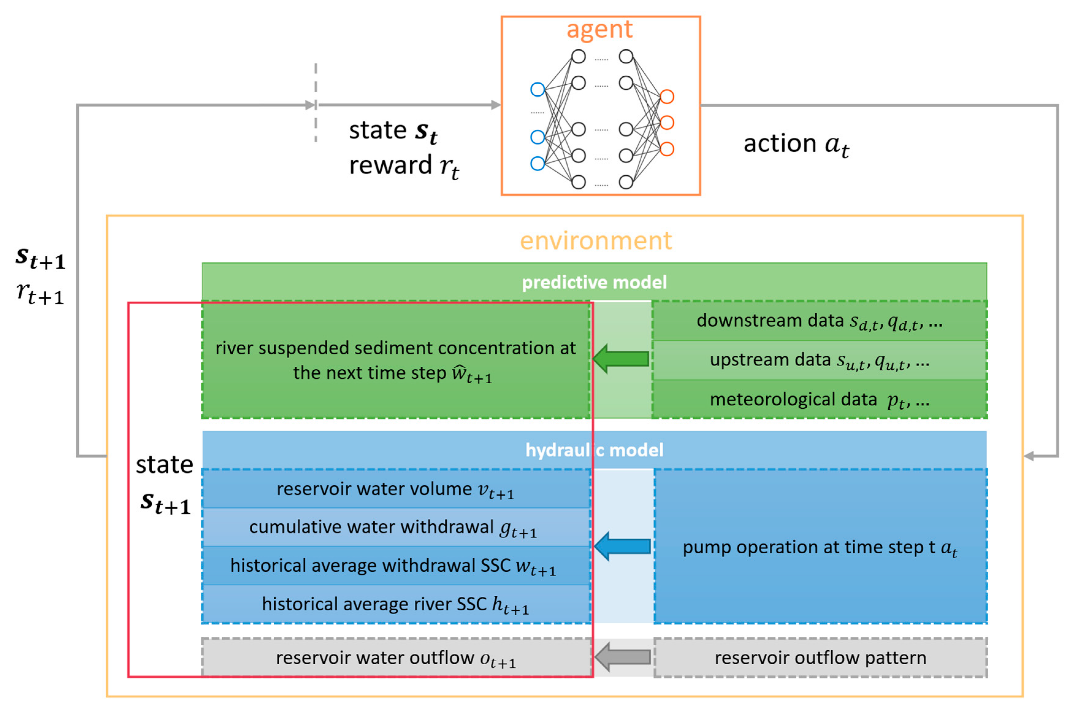
The raw water system in this study consists of an intake pumping station, an off-channel reservoir, and pipes that connect the reservoir and the pumping station. The overall architecture of the proposed DRL-based online control model is illustrated in Figure 1. The action of the system $a_t$ is defined as the pump operation at time step $t$. The state of the system includes the volume of water in the reservoir $v$, the cumulative volume of water withdrawn from the river $g$, the average sediment content of the water withdrawn from the river $w$, the historical average sediment content of the river $h$ and so on. The current state ${\mathit{s}}_{\mathit{t}}$ is the basis for decisions on future actions, and the action chosen in turn affects the state of the system at the next time step. Because the river SSC at the next time step is mainly influenced by the river hydrology, two modules (the hydraulic model and the SSC predictive model) are used to calculate the state transition process of the system, which serve as the environment for reinforcement learning. The hydraulic model is used to calculate the state vectors including reservoir water volume $v_{t+1}$, the cumulative water withdrawal $g_{t+1}$ and other variables. Using the flow, the SSC and other relevant data upstream and downstream of the water intake, the SSC prediction model predicts the SSC of intake water at the next time step. The outputs of the preceding two modules are combined to form the state ${\mathit{s}}_{\mathit{t}\mathbf{+}\mathbf{1}}$ that is used as the basis for control decisions $a_{t+1}$ at the next time step $t+1$.

The DRL agent controls the environment through a closed-loop framework. When the agent performs an action $a_t$ at time $t$, the environment model is used to calculate state ${\mathit{s}}_{\mathit{t}\mathbf{+}\mathbf{1}}$ at next time$t+1$. During the training stage, the agent is trained step by step how to perform actions with a higher cumulative reward. The trained agent is then used to produce the operational strategy for online control.

The robustness of the reinforcement learning framework to uncertain data is validated by comparing three different types of operation strategies, as defined below.

• Manual strategy: the actual pumping station control strategy developed through the experience of human operators.
• Predictive control strategy: with a predicted river SSC, the strategy generated by the DRL-based predictive online control model framework.
• Perfect predictive control strategy: the strategy generated by training with the real-world river SSC. The robustness of the reinforcement learning framework to uncertain data is verified by comparing the test performance of the two strategies (predictive control strategy and perfect predictive control strategy). Perfect predictive control strategy is impractical because it is impossible to make unbiased predictions of the river’s SSC, and it is precisely the future river SSC that influences the choice of control action.

Furthermore, we construct several different online control models and related training datasets under various reservoir outflow patterns and initial reservoir volumes, and examine how these boundary conditions affect the strategies.

2.1. Hydraulic Model

The following are the approximation functions (characteristic curves) between the head of the $H\left(\mathrm{m}\right)$, pump efficiency $\eta (\%)$, and pump flow $q\left({\mathrm{m}}^3/\mathrm{s}\right)$:

$$\begin{array}{c}H=a_{1}q+a_{2}q+a_3\end{array}$$

(1)

$$\begin{array}{c}\eta =b_{1}q+b_{2}q+b_3\end{array}$$

(2)

where $a_1,a_2,a_3,b_1,b_2,b_3$ are constant coefficients.

The system curve head includes the sum of the net pump head and pipeline head loss.

$$\begin{array}{c}H=H_{st}+{{\displaystyle \sum }}^{}{h}_f+{{\displaystyle \sum }}^{}{h}_j\end{array}$$

(3)

where $H_{st}$ is the difference in height between the level of the suction well and the level of the tank. ${{\displaystyle \sum }}^{}{h}_f$ and ${{\displaystyle \sum }}^{}{h}_j$ are the frictional head loss and the minor head loss, respectively. ${{\displaystyle \sum }}^{}{h}_j$ is estimated as 10% of ${{\displaystyle \sum }}^{}{h}_f$ in this study. And ${{\displaystyle \sum }}^{}{h}_f$ is calculated using Equation (4).

$$\begin{array}{c}{{\displaystyle \sum }}^{}{h}_f=10.294n^2\frac{q_s^{2}L}{D^{5.333}}\end{array}$$

(4)

where $q_s$ (${\mathrm{m}}^3/\mathrm{s}$) is the flow rate; $D$ (m) is the inner diameter of the pipe; $L$ (m) is the length of the pipe; $n$ (dimensionless) is the pipe roughness coefficient, set at 0.013 in this study.

The pump operating point is the point at which Equation (1), the pump curve (or parallel combined curve if the pumps are connected in parallel) intersects with Equation (3), the system curve. The above formulas can be used to calculate the flow rate, head, and efficiency of the pump under various operating conditions. The data, such as the daily power of water intake $P_{t+1}\left(\mathrm{kW}\right)$ and the daily water withdrawal $Q_{t+1}\left({\mathrm{m}}^3/\mathrm{d}\right)$, can be further calculated according to the action $a_t$.

$$\begin{array}{c}{P}_t=\frac{\rho gH}{1000\eta }\end{array}$$

(5)

where $\rho$ is the density of the liquid sucked by the pump, set at 1000 $\mathrm{kg}/{\mathrm{m}}^3$ in this study; $g$ is the acceleration of gravity, set at 9.8 $\mathrm{m}/{\mathrm{s}}^2$ in this study; $H$ is the head of the pump and $\eta$ is the pump efficiency, both calculated by pump operating point.

2.2. SSC Predictive Model

To predict the daily average river SSC, a prediction model is built using a multilayer perceptron (MLP). The feedforward neural network consists of one input layer, one hidden layer, and one output layer, with the number of hidden layer neurons determined through trial and error. The output of each neuron is calculated using $\mathrm{LeakRelu}$ as the activation function of the hidden layer [51]. The most recent year of the dataset is used as a test set to evaluate the generalization ability of the predictive models and for comparison with manual strategy. A portion of the data (90%) from the remaining years in the dataset is used for training, while 10% for validation. Training and validation data are both used to generate DRL training data and to train pumping station abstraction strategies.

Daily average flow and daily average SSC from two hydrographic stations upstream and downstream, daily average temperature and rainfall are considered as input variables influencing the SSC of water intake. To analyze the data correlations between those variables, mutual information (MI) [52] and Spearman’s rank correlation coefficient ($r_s$) are used.

Moreover, the original dataset consists of variables with different physical meanings and units, resulting in a highly variable range. The variables are rescaled to $\left[0,1\right]$ in the model preprocess using Equation (6) to ensure that different variables are treated equally in the model and to eliminate their physical dimensions [53]:

$$\begin{array}{c}{x}_{in}=\frac{x_i-x_{imin}+\epsilon }{x_{imax}-x_{imin}+\epsilon } \end{array}$$

(6)

where $x_{in}$ is the rescaled value of variable $i$, $x_i$ is the original value, and $x_{imax}\mathrm{and}{x}_{imin}$ are the maximum and minimum of variable $i$, respectively. $\epsilon$ is a small positive value used to avoid zero values, set at 0.0001 ($x_{imax}+x_{imin}$) in our study.

The performance of the prediction models is evaluated using the root mean square error (RMSE) and the mean absolute error (MAE). The formulas of evaluation metrics are shown in the following Equations (7) and (8).

$$\begin{array}{c}RMSE=\sqrt{\frac{1}{N}{\displaystyle {\displaystyle \sum }_{i=1}^N}{\left(SS{C}_{i,measured}-SS{C}_{i,predicted}\right)}^2}\end{array}$$

(7)

$$\begin{array}{c}MAE=\frac{1}{N}{\displaystyle {\displaystyle \sum }_{i=1}^N}|SS{C}_{i,measured}-SS{C}_{i,predicted}|\end{array}$$

(8)

where $SS{C}_{measured}$ is measured suspended sediment concentration, $SS{C}_{predicted}$ is predicted suspended sediment concentration using the MLP model, and N is the number of data points.

2.3. DRL Agent

Single-agent reinforcement learning is modeled using a Markov Decision Process (MDP), typically the MDP is defined by $\left(S,A,P,R\right)$. S is the set of all environmental states, and $s_t\in S$ denotes the state of the environment at time step $t$. A is the set of all agent actions, and $a_t\in A$ denotes the action taken by the agent at time step $t$. $P:S\times A\times S\to \left[0,1\right]$ is state-transition probability. $R:S\times A\to ℝ$ denotes the scalar signal $r_{t+1}$ received at state $s_t$. The reward $r_{t+1}$ obtained by executing action $a_t$, and an immediate feedback reward is received at each time step until the final time step T. The agent’s objective is to maximize the cumulative rewards it receives over the long term. The sum of the rewards from step $t$ to the final step T is defined as return $G_t$

$$\begin{array}{c}{G}_t={\displaystyle {\displaystyle \sum }_{k=0}^T}{\gamma }^k{r}_{t+k+1}\end{array}$$

(9)

where discount rate $\gamma \in \left[0,1\right]$, used to indicate the present value of future rewards [54].

2.3.1. Action Space

For fixed-speed pumping stations, all possible pump opening combinations can be pre-enumerated. If the total number of all possibilities is $n$, then the discrete action space $A=\left\{0,1,2,\dots ,n-1\right\}.$

2.3.2. State Space

The environmental state includes reservoir water volume $v_t\left({\mathrm{m}}^3\right)$, cumulative water withdrawal $g_t\left({\mathrm{m}}^3\right)$, historical average withdrawal SSC $w_t\left(\mathrm{kg}/{\mathrm{m}}^3\right)$, historical average river SSC $h_t\left(\mathrm{kg}/{\mathrm{m}}^3\right)$, river daily SSC ${\widehat{w}}_t\left(\mathrm{kg}/{\mathrm{m}}^3\right)$, and reservoir water outflow $o_t\left({\mathrm{m}}^3/\mathrm{d}\right)$. ${\widehat{w}}_t$ is predicted by the prediction model. $o_t$ is ideally equal to the daily total surface water consumption; to avoid uncertainty caused by water consumption forecasts, the previous day’s urban water consumption is used in this study instead of the daily total surface water consumption. The calculation of $v_t$ takes into account the reservoir water outflow $o_t$, the pump station water withdrawal $Q_t$ and the reservoir evaporation. The input state ${\mathit{s}}_{\mathit{t}}$is a six-dimensional vector which contains the above states. These are updated at each time step of the model.

$$\begin{array}{c}{\mathit{s}}_{\mathit{t}}=\left(v_t,g_t,w_t,h_t,{\widehat{w}}_t,o_t\right)\end{array}$$

(10)

2.3.3. Reward Function

The reward function is usually used to evaluate the performance of a control strategy. The calculation of the reward at time step$t+1$ in this study depends on the state ${\mathit{s}}_{\mathit{t}\mathbf{+}\mathbf{1}}$ and the action $a_t.$

$$\begin{array}{c}{r}_{t+1}=c_1{r}_{t+1,water}+c_2{r}_{t+1,rule}+c_3{r}_{t+1,reservoir}+c_4{r}_{t+1,power}\end{array}$$

(11)

where $c_1$, $c_2$, $c_3$, and $c_4$ are the weights of the $r_{t+1,water}$, $r_{t+1,rule}$, $r_{t+1,reservoir}$, and $r_{t+1,power}$, respectively.

The water withdrawal reward $r_{t+1,water}$ in Equation (11) reflects the advantages and disadvantages of water quantity and SSC in water withdrawal, which can be represented by:

$$\begin{array}{c}{r}_{t+1,water}=-Q_{t+1}\left({\widehat{w}}_{t+1}-w_{t+1}\right)\end{array}$$

(12)

The threshold $w_{t+1}$ represents the average of the historical SSC of the water withdrawn before time step $t+1$. When ${\widehat{w}}_{t+1}$ is less than $w_{t+1}$, the SSC of the river at this time is lower than in the past. Moreover, the larger the amount of water withdrawal $Q_{t+1}$, the more reward for the agent. When ${\widehat{w}}_{t+1}$ is greater than $w_{t+1}$, it is probably not suitable for large amounts of water withdrawal. The higher the SSC is at this time, the larger $Q_{t+1}$, and the larger the penalty for the agent.

Reservoir capacity reward $r_{t+1,rule}$ is to limit reservoir operation. The reservoir volume must be kept between the maximum storage capacity $v_{max}$ and the dead storage capacity $v_{min}$. If the water volume exceeds $v_{max}$ or fails below $v_{min}$, a penalty proportional to the reservoir volume offset will be imposed.

$$r_{t+1,\mathit{rule}}=\left\{\begin{array}{cc}{v}_{t+1}-v_{\mathit{min}}\hfill & \hspace{1em}{v}_{t+1}<v_{\mathit{min}}\\ v_{\mathit{max}}-v_{t+1}\hfill & \hspace{1em}{v}_{t+1}>v_{\mathit{max}}\\ \hspace{1em}0\hfill & \hspace{1em}\mathit{otherwise}\end{array}\right.$$

(13)

Reservoir remaining water reward $r_{t+1,reservoir}$ is to meet the demand for the urban water consumption, which is presented as a step function.

$$\begin{array}{c}{r}_{t+1,reservoir}={\displaystyle {\displaystyle \sum }_{k=0}^{+\infty }}\ln (k{\epsilon }_1+{\epsilon }_2){\mathcal{X}}_{\left[k{\epsilon }_1,\left(k+1\right){\epsilon }_1\right)}\left(\mathsf{\alpha }\right)\end{array}$$

(14)

where ${\mathcal{X}}_Z\left(\alpha \right)=\{\begin{array}{c}1, \alpha \in Z\\ 0, \alpha \notin Z\end{array}$, ${\epsilon }_1$ is the length of the interval, set at 5 in this study; ${\epsilon }_2\in \left(0,1\right)$ plays the role of punishing low water volume.

$$\begin{array}{c}\alpha =\frac{v_{t+1}-v_{min}}{o_{t+1}}\end{array}$$

(15)

where the reservoir residual indicator $\alpha$ indicates the approximate number of days that the remaining water in the reservoir can be used by the residents. $o_{t+1}$ is used to represent the average level of recent surface water consumption.

To ensure the reliability of water supply when there is a low amount of water available in the storage reservoir, i.e., when $\alpha$ is less than 15, $r_{t+1,water}=\max \left(0,-Q_{t+1}\left({\widehat{w}}_{t+1}-w_{t+1}\right)\right)$, which means the penalty due to high SSC in the abstracted water is no longer calculated at this time.

Energy consumption incentive $r_{t+1,power}$ calculates the effective power saved by monthly water withdrawal.

$$\begin{array}{c}{r}_{t+1,power}=P_{threshold}-{\displaystyle {\displaystyle \sum }_{t=1}^T}{P}_{t+1}/Q_{t+1}\end{array}$$

(16)

where $P_{threshold}$ is a threshold value to avoid the appearance of extremely large energy consumptions, set at 110 $\mathrm{kWh}/{\mathrm{km}}^3$ in this study. The daily total power of water intake $P_{t+1}\left(\mathrm{kW}\right)$ and the daily total water withdrawal $Q_{t+1}\left({\mathrm{m}}^3/\mathrm{d}\right)$ can be calculated by the hydraulic model.

2.3.4. Training Method and Process

In this study, proximal policy optimization (PPO) [55] is used to train the DRL agent. PPO is a policy gradient approach that uses a deep neural network to approximate policy function and uses stochastic gradient ascent to optimize the objective function through interactive data sampling with the environment. Policy gradient methods are very popular in reinforcement learning, they can optimize the cumulative reward directly with nonlinear function approximators such as neural networks. Standard policy gradient methods perform one gradient update per data sample, while PPO proposes an objective function which enables multiple epochs of minibatch updates.

$$\begin{array}{c}\underset{\theta }{\mathrm{maximize}}{\widehat{\mathbb{E}}}_t\left[\min (r_t\left(\theta \right){\widehat{A}}_t,\mathrm{clip}\left(r_t\left(\theta \right),1-ϵ,1+ϵ){\widehat{A}}_t\right)\right] \end{array}$$

(17)

where $r_t\left(\theta \right)$ denotes the probability ratio $r_t\left(\theta \right)=\frac{{\pi }_{\theta }\left(a_t|s_t\right)}{{\pi }_{{\theta }_{old}}\left(a_t|s_t\right)}$, where ${\pi }_{\theta }\left(a_t|s_t\right)$ is a policy function obtained by neural network with parameter $\theta$. ${\widehat{A}}_t$ is an estimator of the advantage function at timestep $t$. The advantage function measures whether or not the action is better or worse than the policy’s default behavior [56], and $ϵ$ is the clipping parameter.

The time step of the environmental simulation is one day, and each episode is simulated from the beginning of the year to the end of the year. For each episode, the learning process of the agent is as follows:

• Initialize the simulation environment and return the initial state (randomly select a year from the training dataset as the hydrological year $Y_{hy}$ of this episode; randomly select a year from the training dataset as the water consumption year $Y_{wc}$ of this episode; randomly sample a reservoir water volume as the annual initial reservoir volume $v_0$).
• For each time step:

  (a)

  Sample of actions from the control strategy according to the state ${\mathit{s}}_{\mathit{t}}$ at the current time step;

  (b)

  Apply action $a_t$ to the simulated environment, and this action will affect the state ${\mathit{s}}_{\mathit{t}\mathbf{+}\mathbf{1}}$ at the next step. Part of the state changed by the action is calculated using the hydraulic model; the rest of the state not related to the action is updated using the prediction model;

  (c)

  Calculate the reward $r_{t+1}$;

  (d)

  Store the data sample [${\mathit{s}}_{\mathit{t}}$, $a_t$, ${\mathit{s}}_{\mathit{t}\mathbf{+}\mathbf{1}}$, $r_{t+1}$] into the training dataset.

• Update the parameters of the DRL agent using the PPO algorithm.

3. Case Study

3.1. Raw Water System of the Study Area

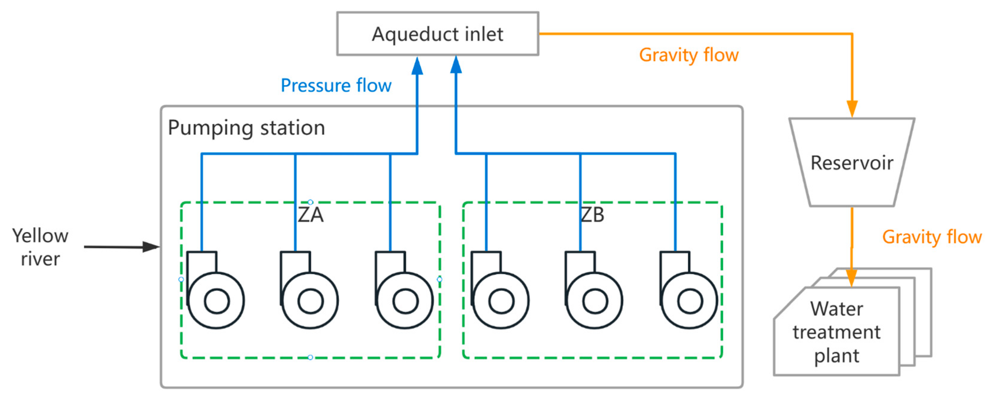
The Yinchuan water supply system was selected as a case study. The pumping station was built on the left bank of Jinshawan, upstream of Qingtongxia Conservancy Hub on the Yellow River. As shown in Figure 2, the pumping station has six fixed-speed centrifugal pumps of the same type. Each of the three pumps at the pumping station has a common outlet pipe that enters the Xixia Aqueduct’s inlet via 5.3 km of DN2600 steel-wound concrete pressure pipeline and then gravity feeds water to the storage reservoir via 65.2 km of the Xixia Aqueduct. Raw water from the reservoir is then transferred by gravity to the water treatment plants.

3.2. Modeling

This case study applies several assumptions and presets: (1) because the static head of pumps is fixed, the hydraulic model can calculate different pump combinations in advance, simplifying the action space; (2) one year of water consumption data-added Gaussian noise are used for training, while another year of real water consumption data are used to test; and (3) because the water intake of the pump station is very close to the downstream hydrological station, the downstream station’s hydrological data is used to approximate the ones at the water intake.

3.2.1. Simplify the Action Space

The approximation functions (pump curve) between the head of the pump $H$, pump efficiency $\eta$, and pump flow rate $q$ are as follows:

$$\begin{array}{c}H=-0.41q^2-2.2674q+54.161\end{array}$$

(18)

$$\begin{array}{c}\eta =-3.4688q^2+34.876q+2.3286\end{array}$$

(19)

The ${{\displaystyle \sum }}^{}{h}_f$ in Equation (4) is calculated by:

$$\begin{array}{c}{{\displaystyle \sum }}^{}{h}_f=10.294n^2\frac{q_s^{2}L}{D^{5.333}}=10.294\times {0.013}^2\times 5342\times \frac{q_s^2}{{2.6}^{5.333}}\end{array}$$

(20)

As illustrated in Figure 2, the six pumps of the pumping station are divided into two hydraulically equivalent zones $\mathrm{ZA}$ and $\mathrm{ZB}$, where three pumps in zone $\mathrm{ZA}$ share a common outlet pipe and three pumps in zone $\mathrm{ZB}$ share another outlet pipe. The eight possible combinations of actions for the pumping station are summarized in

Table 1. Water pump opening combinations.

Number of Pumps On	Possible Pump Combinations	Energy Consumption per Unit of Water Intake $\left(\mathbf{k}\mathbf{W}\mathbf{h}/\mathbf{k}{\mathbf{m}}^3\right)$	Average Pump Efficiency $\left(\mathbf{\%}\right)$	Pump Combination after Simplifying the Action Space
0	No pump on	0	-	No pump on
1	$\mathrm{ZA}1$	99.7	89.74	$\mathrm{ZA}1$
2	$\mathrm{ZA}2$	113.8	90.04	$\mathrm{ZA}1+\mathrm{ZB}1$
	$\mathrm{ZA}1+\mathrm{ZB}1$	99.7	89.04
3	$\mathrm{ZA}3$	129.9	86.97	$\mathrm{ZA}1+\mathrm{ZB}2$
	$\mathrm{ZA}1+\mathrm{ZB}2$	108.7	89.71
4	$\mathrm{ZA}1+\mathrm{ZB}3$	120.8	87.66	Z $\mathrm{A}2+\mathrm{ZB}2$
	$\mathrm{ZA}2+\mathrm{ZB}2$	113.8	90.04

Note: Taking opening two pumps for example, $\mathrm{ZA}2$ represents opening two pumps in the $\mathrm{ZA}$ area, while $\mathrm{ZA}1+\mathrm{ZB}1$ represents opening one pump each in $\mathrm{ZA}$ and $\mathrm{ZB}$.

. Some pump combination operations with significantly high energy consumption are directly excluded. By action space simplification, there are a total of five possible ways of opening the pumping station, i.e., $a_t\in \left\{0,1,2,3,4\right\}$.

3.2.2. Water Consumption Data

Surface water from the Yellow River has been used inconsistently in Yinchuan, where surface water gradually replaced groundwater as a source of drinking water over the last decade. A relatively stable period of water consumption data from 1 January 2021 to 31 December 2021 is used for analysis. Figure 3a shows the fluctuation of the daily water consumption. Following assumption (2), Gaussian noise $X~\mathcal{N}\left(\mu ,{\sigma }^2\right) \left(\left|\mu \right|\le 2.5\times {10}^4{\mathrm{m}}^3/\mathrm{d},\sigma \le 2\times {10}^4{\mathrm{m}}^3/\mathrm{d}\right)$ is added to the water consumption data of 2021 for training, and for testing the actual data without noise is used. To initialize the simulation environment, we use the randomly sampled data that follows the Gaussian noise distribution as the daily water consumption $Y_{wc}$ (Figure 3b). The choice of Gaussian noise parameters is based on the analysis of the data characteristics.

3.2.3. SSC Forecasting

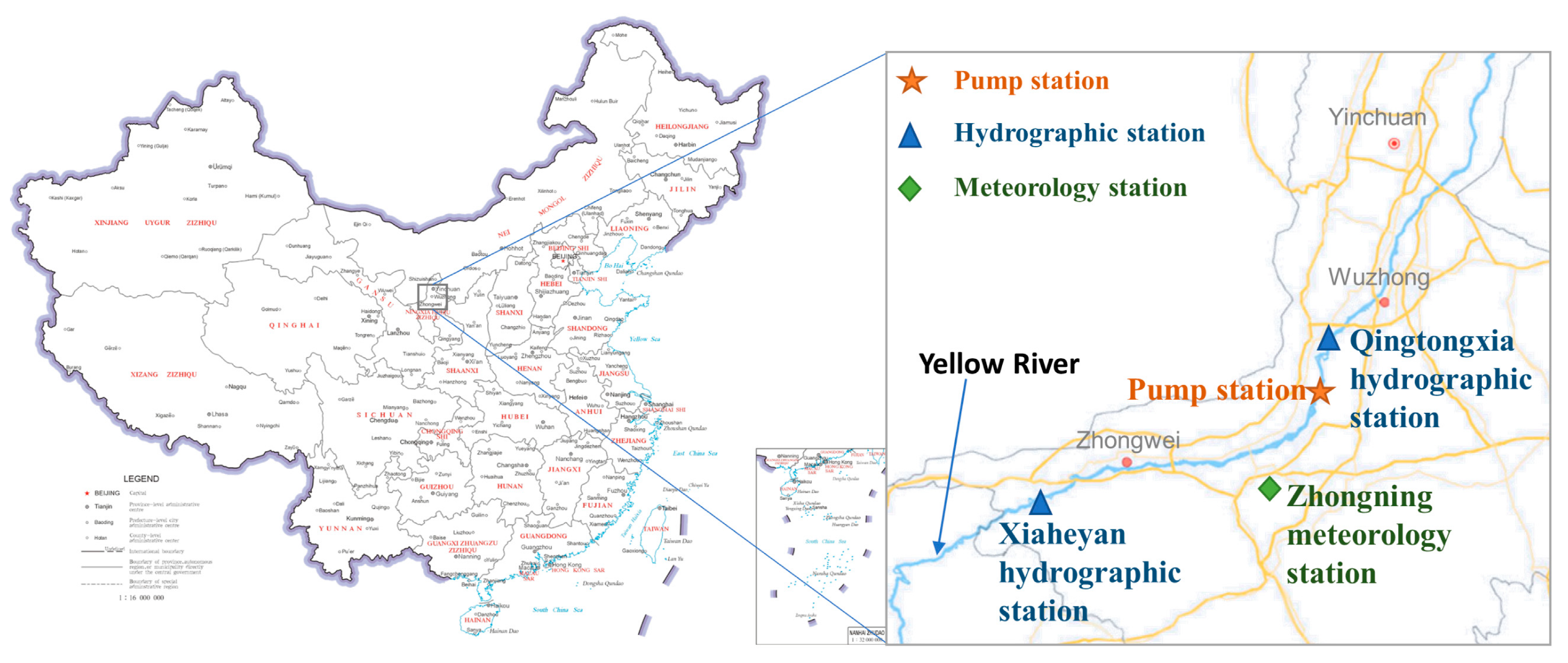
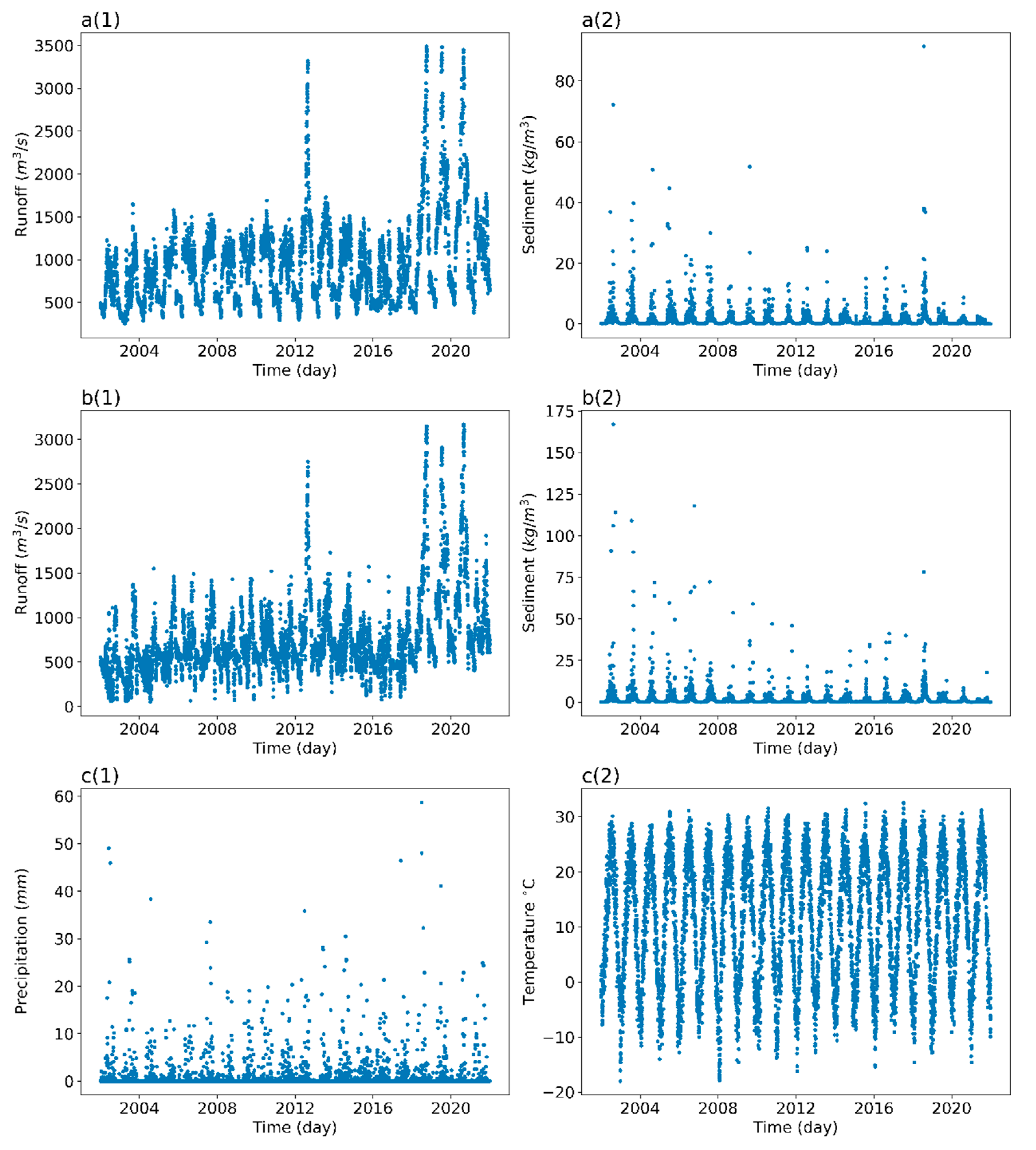
Data from two hydrographic stations upstream and downstream of the Yellow River intake section (Xiaheyan hydrographic station upstream and Qingtongxia hydrographic station downstream, respectively), and one meteorology station (Zhongning station) are used to predict the SSC at the water intake of the pump station. Figure 4 shows the location of the stations. The meteorological data was downloaded from the National Oceanic and Atmospheric Administration (NOAA) website. Figure 5 shows the data for the three stations from 2002 to 2021.

Some researchers have demonstrated that flow and SSC correspond differently under different runoff patterns influenced by rainfall, climate, and sediment sources [57]. During the freezing period, the water flow has a reduced ability to hold sand and the SSC is smaller. During the non-freezing period, the SSC of the river mainly depends on rainfall erosion, river runoff, the sand transport capacity of the water flow, and river scouring. Therefore, the prediction models are established separately for the freezing and non-freezing periods.

Table 2. Input variables and partial parameters of the predictive model.

Model	Input Variables $\mathit{I}\mathit{n}\mathit{p}\mathit{u}\mathit{t}$	Number of Input Layer Neurons	Number of Hidden Layer Neurons
non-freezing period model	$month,s_{d,t-1},s_{d,t-2},s_{u,t-1},q_{u,t-1},q_{d,t-1},p_{t-1},p_{t-2}$	8	12
freezing period model	$month,s_{d,t-1},s_{d,t-2},s_{u,t-1},q_{u,t-1},q_{d,t-1}$	6	10

provides the model input variables and hidden layer neuron parameters of the SSC predictive models. The number of hidden layer neurons is selected from eight to 16 by the trial-and-error method. The variables are downstream river SSC $s_d$, upstream river SSC $s_u$, downstream flow $q_d$and upstream flow $q_u$. The daily rainfall data $p$ mainly influences the SSC in the non-freezing period.

3.2.4. DRL Configuration

Parameter settings of the deep reinforcement learning network are shown in

Table 3. Parameters of the deep reinforcement learning network.

Variable	Value
Num iterations	300 k
Timesteps per update	840
Batch size	420
Adam step size	$1\times {10}^{-4}$
Clipping parameter ($ϵ$)	0.2
Discount ($\gamma$)	0.99
GAE parameter ($\lambda$)	0.95

; the meaning of each parameter is found in the literature [55]. The computer used in this study was Intel(R) Xeon(R) Gold 6230 R CPU running at 2.10 GHz and GeForce_RTX_3090 GPU, and the RAM available was 32 GB. The number of iterations was set to 300 k, and it delays approximately twenty minutes to converge to the solution.

3.3. Predict Model Performance

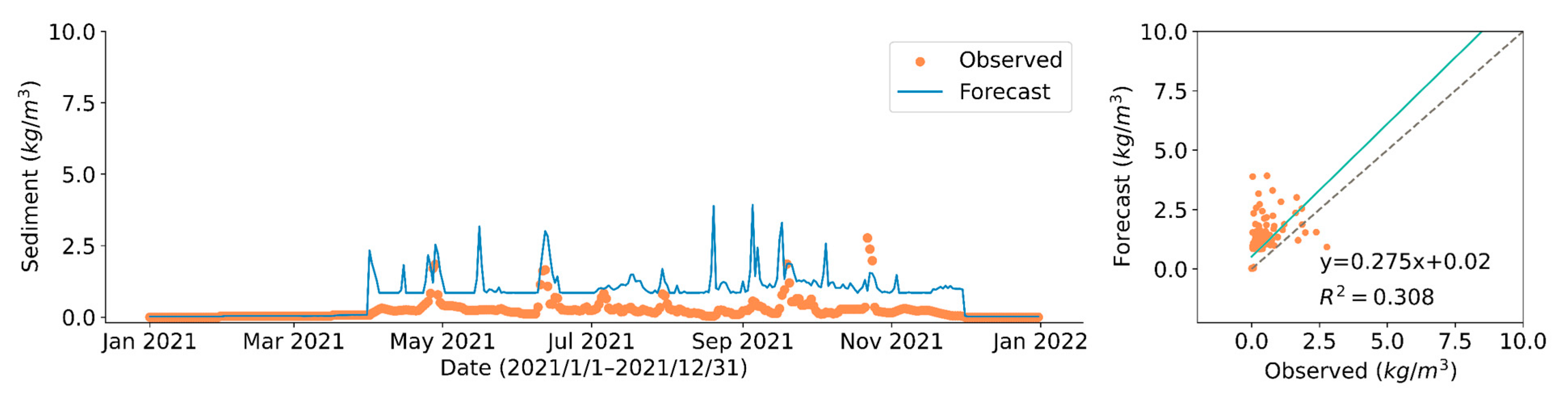
The performance of the prediction models is evaluated using RMSE and MAE, as shown in Figure 6 and

Table 4. Comparison of model performance.

	Model	Training Set	Validation Set	Test Set
$\mathrm{RMSE}\left(\mathrm{kg}/{\mathrm{m}}^3\right)$	non-freezing period	4.317	2.942	0.948
	freezing period	0.023	0.024	0.016
$\mathrm{MAE}\left(\mathrm{kg}/{\mathrm{m}}^3\right)$	non-freezing period	1.140	1.007	0.837
	freezing period	0.008	0.009	0.013

. The Qingtongxia Water Conservancy Hub, located 12 $\mathrm{km}$ downstream of the intake, discharges sand and water once a year for two to three days to reduce sediment deposition in the reservoir. The flow velocity increases and the SSC increases significantly around the water intake station during the sand discharge period. Since the hydraulic hub scheduling information can be known in advance, the SSC data due to this unnatural hydrological process are pre-processed as outliers in the model prediction.

The overall distribution of SSC in the test year differs significantly from the data in the training and validation sets, and the SSC regularity is not strong. Although the deviation of the predicted value from the true value in a single step is large, the error compensation mechanism used in the DRL framework can transform the long-term cumulative state deviation of the system as small as possible. It can be seen from the results of Section 3.4 that the reinforcement learning strategy can still achieve near-optimal performance despite the large prediction deviation.

3.4. Results of the DRL

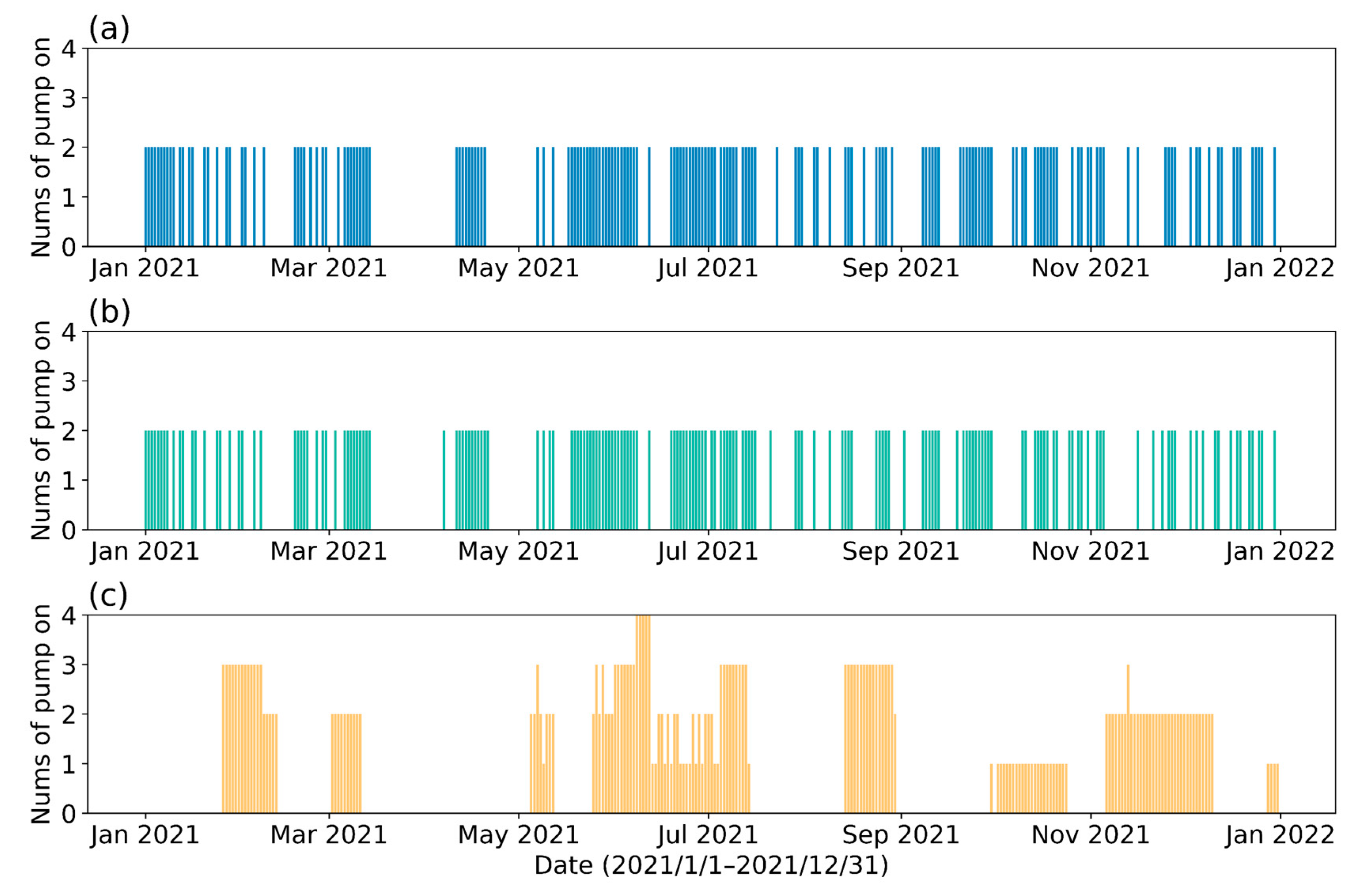
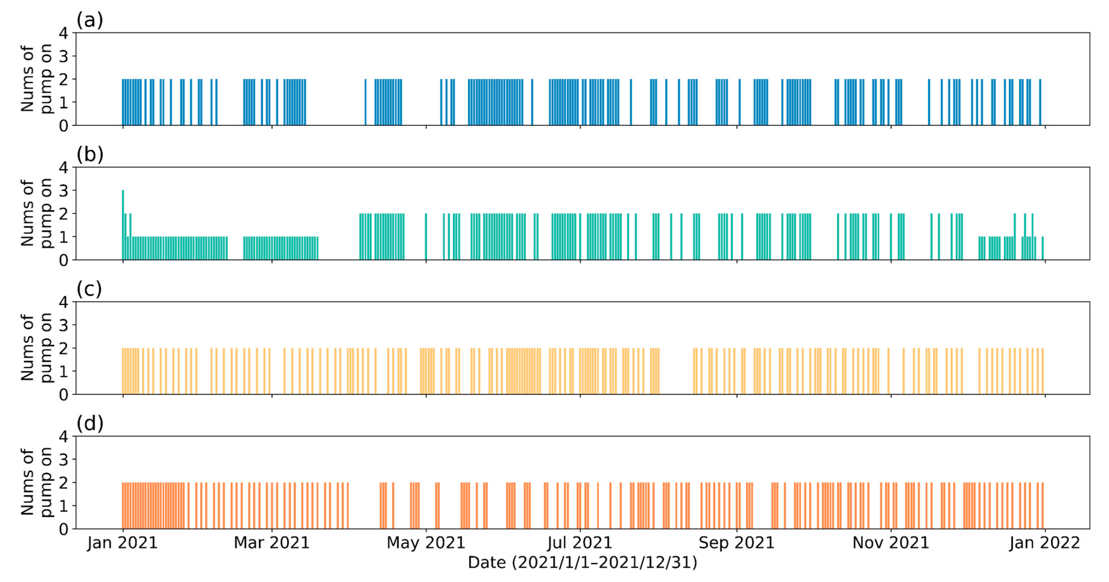
Figure 7 illustrates the number of pumps that are activated per day for different control strategies. The manual strategy and the two control strategies derived from DRL training differ significantly. The manual strategy selects more intensive pump turn-on times, with pumps turned on intensively in June, August, and November, but very few or no pumps are activated in April and September. In contrast, the DRL strategies prefer to turn on the pumps more frequently for water intake during the winter, and they prefer to reduce the number of days of raw water abstraction during seasons when the SSC is higher and uncertainty is greater.

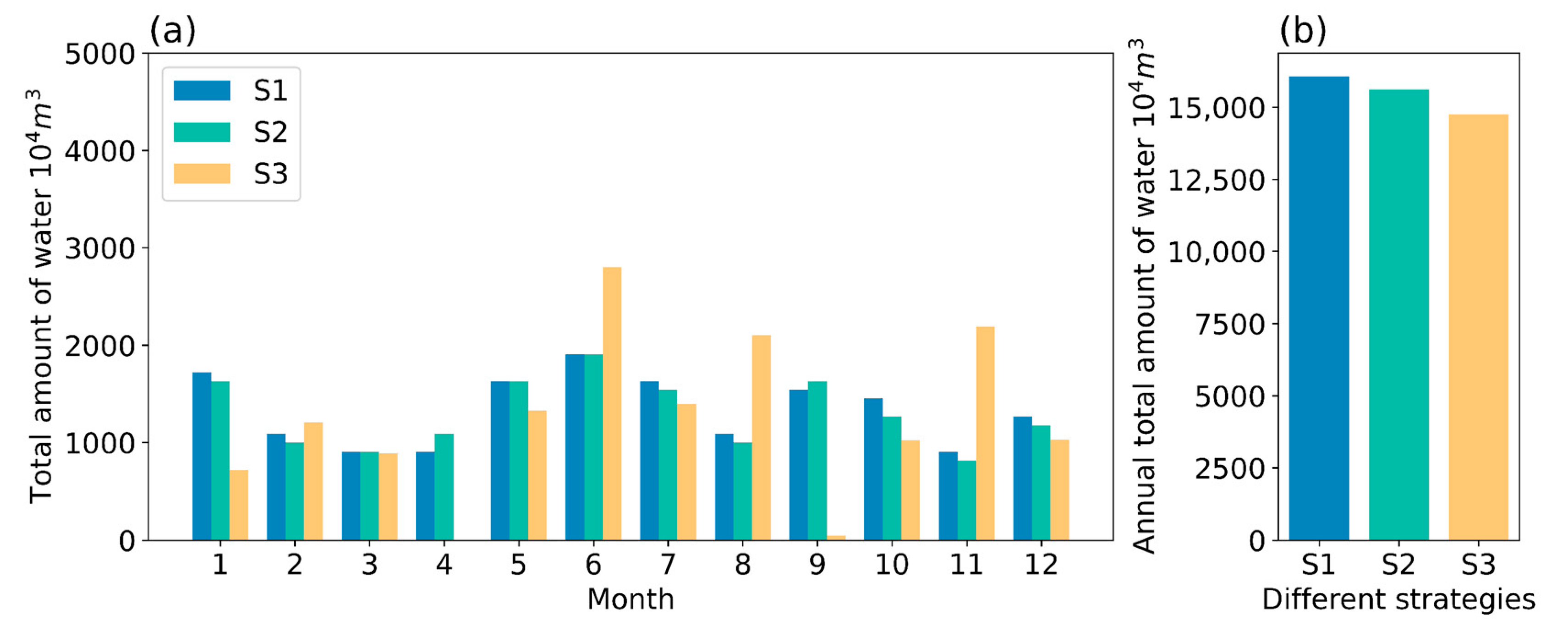
Figure 8 presents an overview of the amount of water withdrawn for different strategies. It can be seen that the total amount of water abstracted for the different strategies is similar throughout the year, which is important and indicates that the water withdrawal strategies we have trained yield a long-term water supply and demand balance without affecting the Yellow River’s ecological system. Since the predictive control strategy has less variation in the amount of water withdrawn each month than the manual strategy, the reservoir water volume fluctuates less.

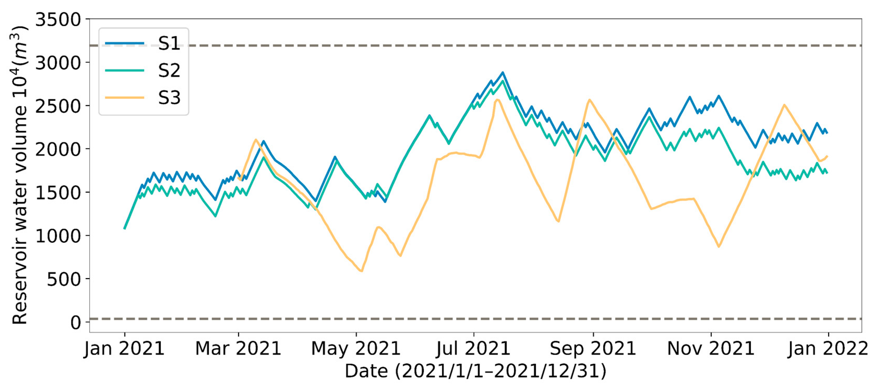
Figure 9 illustrates the change in reservoir water storage. The volumes of water storage at the end of the testing year are different for the three strategies. The reward function is designed in such a way that the predictive control strategies have no violations, such as reservoir water exceeding $V_{min}$ or $V_{max}$ or insufficient reservoir water for urban use. Meanwhile, the reward function keeps a certain amount of reservoir water at the end of the year to prepare for the following year’s schedule. It can also be observed in Figure 9 that the DRL strategies produce less fluctuations on water storage volume throughout the year than the manual strategy.

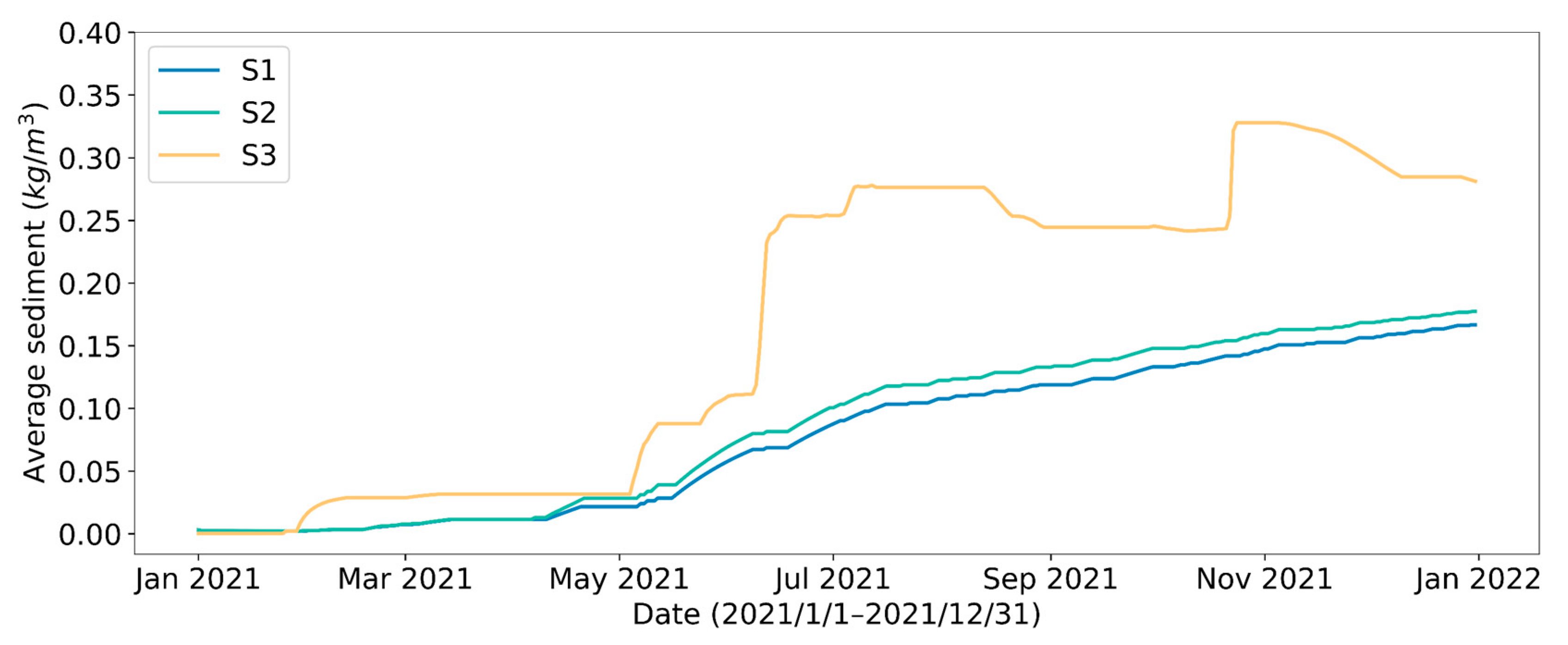
Figure 10 shows the variation in the cumulative average SSC per unit of water abstracted for the different strategies. It could be argued that the positive results are due to the fact that the DRL model is able to predict the future SSC of the river. This enables the strategies to better choose the timing of withdrawals, taking large amounts of water at low SSC and suspending withdrawals at high SSC, significantly reducing the amount of sediment in the annual abstraction and the sedimentation in the reservoir. The result shows that employing a predictive control strategy rather than a manual strategy could reduce sediment content per unit abstraction by 37.01%, while employing a perfect predictive control strategy could reduce sediment content per unit abstraction by 40.57%.

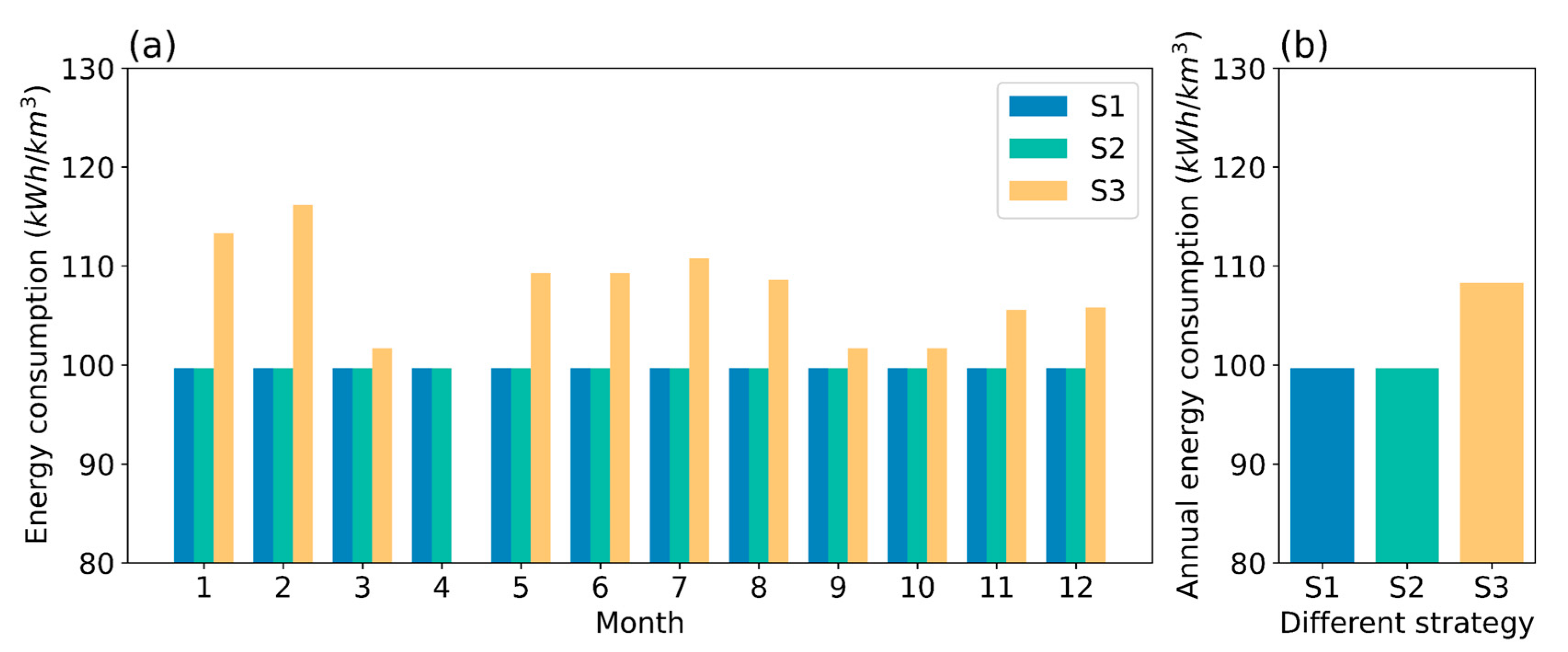
In terms of energy consumption per unit of water withdrawn, predictive control strategies outperform the existing manual strategy. The monthly abstraction energy consumption of the manual strategy ranges from 0 to 3062.78 MWh, and the predictive control monthly abstraction energy consumption ranges from 814.64 to 2081.86 MWh. The perfect predictive strategy is similar to the predictive control strategy, with monthly power consumption ranging from 905.16 to 1991.34 MWh. As can be seen from Figure 11, the predictive control strategy can reduce the energy consumption of water withdrawal. The current manual strategy uses $108\mathrm{kWh}/{\mathrm{km}}^3$ of power per unit of water abstracted throughout the year. Using predictive control strategy can reduce the annual power consumption per unit of water withdrawal by 8.33%.

Finally, the performance of the three strategies is summarized in

Table 5. Summary of water withdrawal performance of different strategies throughout the test year.

Strategy	$\mathbf{Total}\mathbf{Annual}\mathbf{Water}\mathbf{Intake}\left({10}^4{\mathbf{m}}^3\right)$	$\mathbf{Total}\mathbf{Energy}\mathbf{Consumption}\left(\mathbf{M}\mathbf{W}\mathbf{h}\right)$	Energy Consumption per Unit of Water Intake $\left(\mathbf{k}\mathbf{W}\mathbf{h}/\mathbf{k}{\mathbf{m}}^3\right)$	$\mathbf{Total}\mathbf{Sand}\mathbf{Amount}\left({10}^4 \mathbf{k}\mathbf{g}\right)$	$\mathbf{Average}\mathbf{Sand}\mathbf{Volume}\mathbf{per}\mathbf{Unit}\mathbf{of}\mathbf{Water}\mathbf{Withdrawal}\left(\mathbf{k}\mathbf{g}/{\mathbf{m}}^3\right)$
Perfect prediction control	15,980	15,931	99.7(−8.33%)	2679(−35.40%)	0.167(−40.57%)
Predictive control	15,617	15,569	99.7(−8.33%)	2768(−33.25%)	0.177(−37.01%)
Manual control	14,747	15,970	108	4147	0.281

. It demonstrates that there is little difference between the three strategies in terms of annual abstraction volume, which is approximately $1.5\times {10}^8{\mathrm{m}}^3$, but the two DRL strategies perform exceptionally well in terms of energy consumption and sediment content per unit abstraction. This is because the agent is trained to find strategies with a higher cumulative reward, which is reflected in the optimization of energy consumption and fetching water sediment content. The predictive control strategy and the perfect predictive strategy perform equally well in terms of energy consumption per unit of abstracted water. Given the relatively large prediction error of the SSC model, it is encouraging that the predictive control strategy achieves slightly less than perfect results under these conditions, which demonstrates the robustness of the DRL framework in dealing with imperfect data.

4. Results and Discussion

4.1. Effect of Different Reservoir Water Outflow Patterns

Four different patterns of reservoir daily outflow are compared to study the effect of different reservoir operations on training the predictive control strategy, including P1: equal to the water consumption of the previous day, P2: equal to the exact water consumption of the day (assuming we have perfectly predicted the daily water consumption), P3: equal to monthly average water consumption, and P4: equal to annual average surface water consumption. Considering the uncertainties of the daily water consumption, Gaussian noise ($X~\mathcal{N}(\mu ,{\sigma }^2$)) is further added to the daily water consumption data for model training. The influence of the predictive control strategy is as follows.

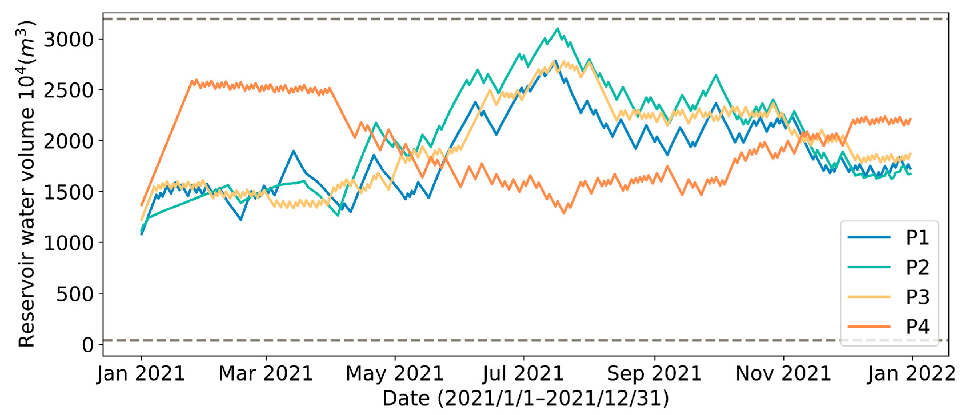
The daily water consumption in Yinchuan City varies greatly, as shown in Figure 3, with a relatively obvious seasonal correlation. In P1 and P2, due to the significantly higher summer reservoir outflow $o_t$ in summer, to ensure that the reservoir is well reliable at all times, it requires more water withdrawals during the periods of peak water consumption (Figure 12, Figure 13 and Figure 14), which inevitably raises the quantity of water abstraction with high SSC (Figure 15). In P4, reservoir outflow remains consistent throughout the year, with a focus on producing large withdrawals in the winter when the SSC is low and avoiding as many as possible withdrawals during the rainy season when the SSC is higher. Despite the different patterns of pump scheduling, the DRL strategies under the four patterns achieve very close output in total annual water intake, as well as energy consumption, as shown in

Table 6. Effect of different reservoir water output patterns on predictive control strategy.

Water Outflow Type	$\mathbf{Total}\mathbf{Annual}\mathbf{Water}\mathbf{Intake}\left({10}^4{\mathbf{m}}^3\right)$	$\mathbf{Total}\mathbf{Energy}\mathbf{Consumption}\left(\mathbf{M}\mathbf{W}\mathbf{h}\right)$	Energy Consumption per Unit of Water Intake $\left(\mathbf{k}\mathbf{W}\mathbf{h}/\mathbf{k}{\mathbf{m}}^3\right)$	$\mathbf{Total}\mathbf{Sand}\mathbf{Amount}\left({10}^4 \mathbf{k}\mathbf{g}\right)$	$\mathbf{Average}\mathbf{Sand}\mathbf{Volume}\mathbf{per}\mathbf{Unit}\mathbf{of}\mathbf{Water}\mathbf{Withdrawal}\left(\mathbf{k}\mathbf{g}/{\mathbf{m}}^3\right)$
P1	15,617	15,569	99.7	2768	0.177
P2	15,561	15,524	99.8	2691	0.173
P3	15,617	15,569	99.7	2808	0.180
P4	15,616	15,568	99.7	2639	0.169

.

Overall, the results indicate that whether the reservoir outflow pattern is the previous day’s or the current day’s daily water consumption has little effect on the predictive control strategy. Different reservoir outflow patterns could be selected based on the water plant’s ability to accept changes in treatment intake, the regulating capacity of the clear water basin, care for the SSC of the abstracted water, and other factors.

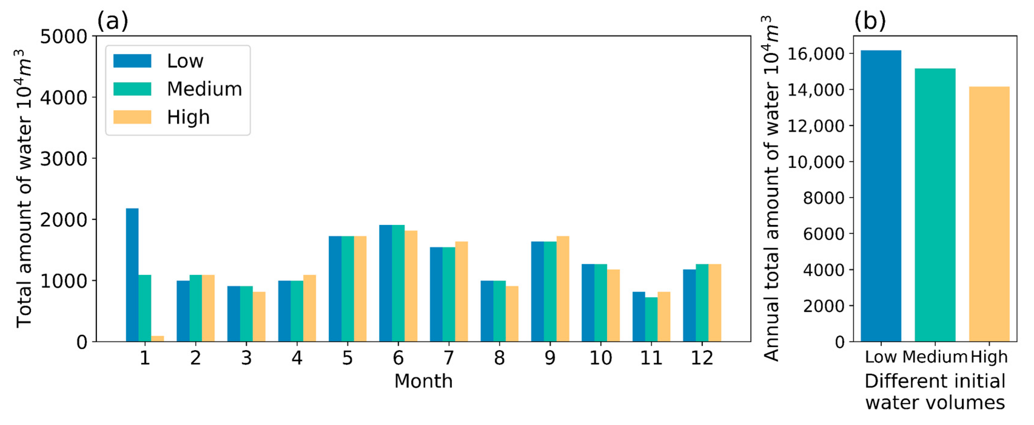
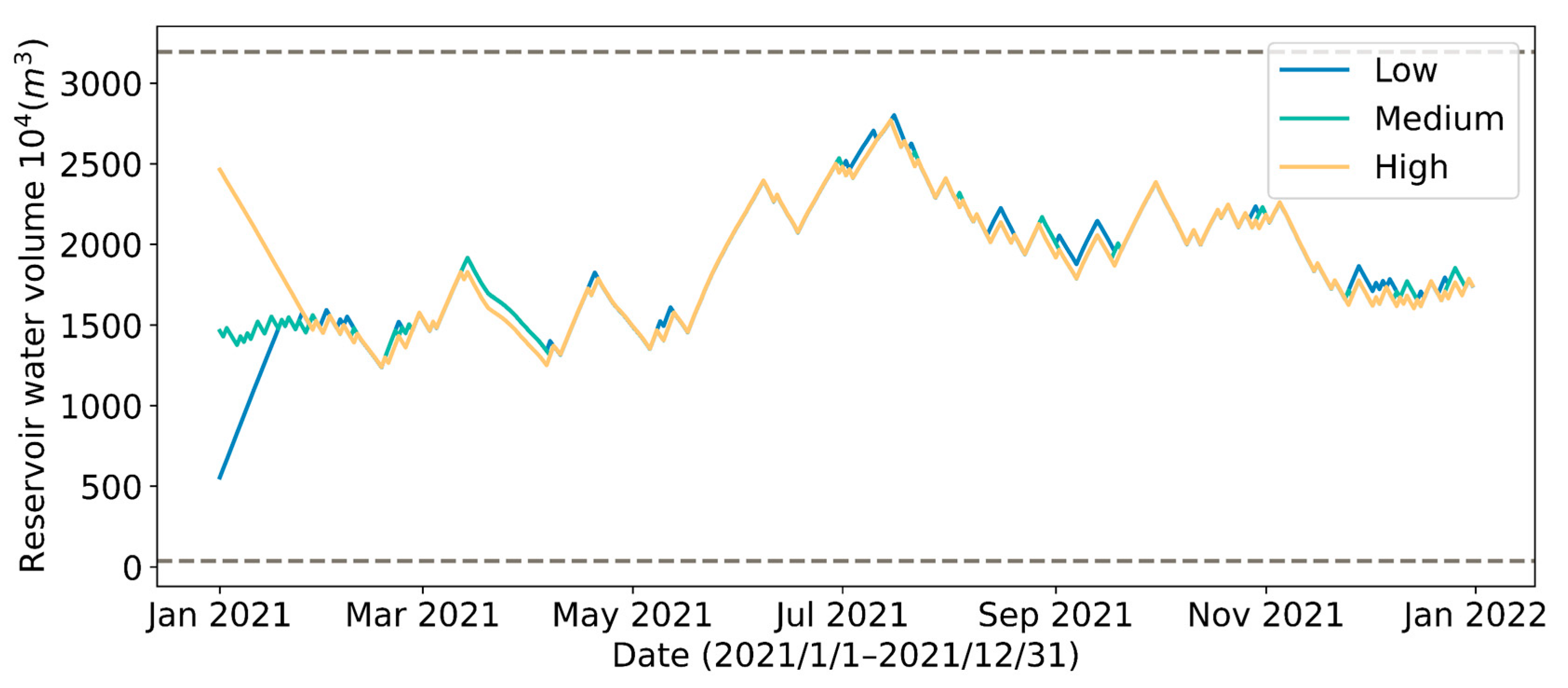
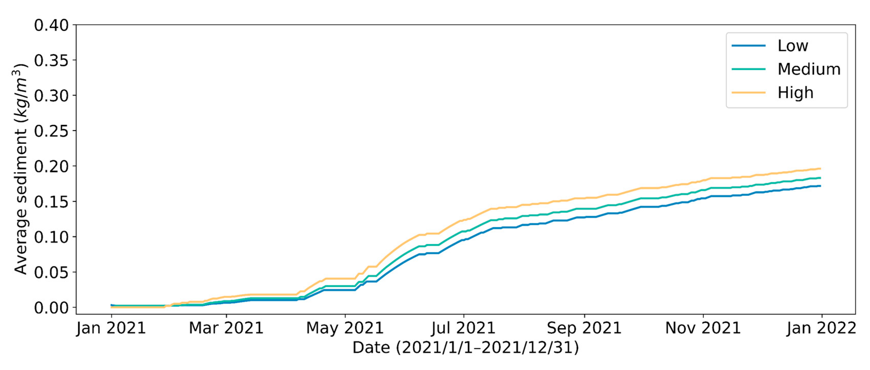
4.2. Effect of Different Initial Reservoir Water Volumes

Three different levels of reservoir water volume at the beginning of the year, low ($500\times {10}^4{\mathrm{m}}^3$), medium ($1500\times {10}^4{\mathrm{m}}^3$), and high ($2500\times {10}^4{\mathrm{m}}^3$) are chosen to explore the effect of different initial reservoir water volumes on the predictive control strategy results.

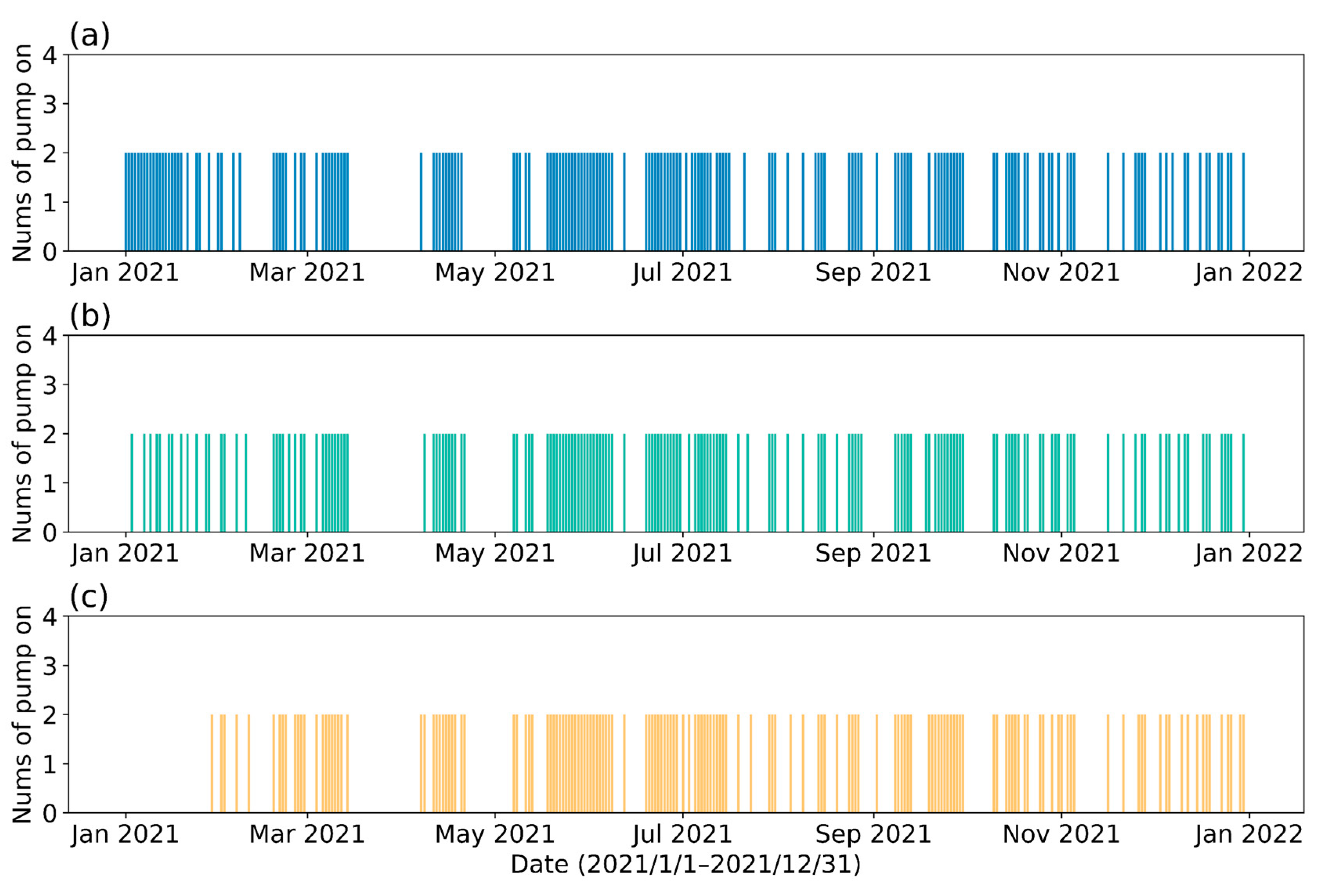
As shown in Figure 16 and Figure 17, different initial reservoir storage volumes primarily influence the result of control strategy in the first month, and have little effect on the remaining months of control strategy. Furthermore, all three predictive control strategies tend to achieve similar reservoir storage volume at the end of the year (Figure 18). Due to the low river SSC in winter, a strategy with low initial reservoir water volume will choose to take a large amount of water right away. Although the total amount of water withdrawn is the least (Figure 17b) in the strategy with high initial reservoir volume, the SSC of water withdrawn is the highest (Figure 19). The results of the analysis are summarized in

Table 7. Effect of different initial reservoir volumes on predictive control strategy.

Initial Reservoir Volume	$\mathbf{Total}\mathbf{Annual}\mathbf{Water}\mathbf{Intake}\left({10}^4{\mathbf{m}}^3\right)$	$\mathbf{Total}\mathbf{Energy}\mathbf{Consumption}\left(\mathbf{M}\mathbf{W}\mathbf{h}\right)$	Energy Consumption per Unit of Water Intake $\left(\mathbf{k}\mathbf{W}\mathbf{h}/\mathbf{k}{\mathbf{m}}^3\right)$	$\mathbf{Total}\mathbf{Sand}\mathbf{Amount}\left({10}^4 \mathbf{k}\mathbf{g}\right)$	$\mathbf{Average}\mathbf{Sand}\mathbf{Volume}\mathbf{per}\mathbf{Unit}\mathbf{of}\mathbf{Water}\mathbf{Withdrawal}\left(\mathbf{k}\mathbf{g}/{\mathbf{m}}^3\right)$
Low	16,161	16,112	99.7	2777	0.172
Medium	15,163	15,116	99.7	2776	0.183
High	14,164	14,120	99.7	2779	0.196

.

4.3. Limitation and Future Work

Although the DRL-based pump scheduling scheme outperforms the current manual strategy, no other optimization methods are compared in this study. In addition, a variety of objectives are considered in the design of the reward function. The effect of different combinations of weight coefficients on the model results are the next research direction for this study.

5. Conclusions

In this study, we created a DRL-based predictive online control framework for the operation of a raw water system fed by a high-sediment river.

In terms of energy consumption and SSC per unit of water withdrawal, the DRL-based predictive control strategy outperforms the manual strategy. It has the potential to reduce the energy consumption of water supply systems and the operation costs of water plants. Furthermore, the reduction of SSC in water withdrawal can significantly extend the service life of storage reservoirs.

Meanwhile, the predictive control strategy performs similarly to the perfect predictive strategy, indicating that the predictive control strategy has good robustness and can still guide the operation of water withdrawal pumping stations relatively well even when SSC prediction is uncertain.

We discussed the effect of reservoir outflow pattern and initial annual reservoir volume on the water withdrawal strategy, in addition to the online control of pumping stations for reservoir abstraction. In fact, the pump online control strategy is heavily influenced by reservoir outflow patterns and reservoir initial water volumes. They both produce good cumulative reward functions, which means that they both reduce energy consumption and abstraction SSC. Different long-term options have different annual abstraction volumes, pumping station scheduling strategies, reservoir operating curves, and so on. In addition to comparing relevant metrics, the operator’s preferences may influence the selection of different reservoir out-flow patterns and initial annual reservoir volumes.

References

- Wee, W.J.; Zaini, N.B.; Ahmed, A.N.; El-Shafie, A. A review of models for water level forecasting based on machine learning. Earth Sci. Inform. 2021, 14, 1707–1728. [Google Scholar] [CrossRef]
- Giuliani, M.; Herman, J.D.; Castelletti, A.; Reed, P. Many-objective reservoir policy identification and refinement to reduce policy inertia and myopia in water management. Water Resour. Res. 2014, 50, 3355–3377. [Google Scholar] [CrossRef] [Green Version]
- Şen, Z. Reservoirs for Water Supply Under Climate Change Impact—A Review. Water Resour. Manag. 2021, 35, 3827–3843. [Google Scholar] [CrossRef]
- Annandale, G.W.; Morris, G.L.; Karki, P. Extending the Life of Reservoirs: Sustainable Sediment Management for Dams and Run-of-River Hydropower; Directions in Development—Energy and Mining; World Bank: Washington, DC, USA, 2016; Available online: https://openknowledge.worldbank.org/handle/10986/25085 (accessed on 8 March 2023).
- Schleiss, A.J.; Franca, M.J.; Juez, C.; De Cesare, G. Reservoir sedimentation. J. Hydraul. Res. 2016, 54, 595–614. [Google Scholar] [CrossRef]
- Annandale, G.W. Quenching the Thirst: Sustainable Water Supply and Climate Change; Create Space Independent Publishing Platform: North Charleston, SC, USA, 2013; p. 250. [Google Scholar]
- Morris, G.L. Classification of Management Alternatives to Combat Reservoir Sedimentation. Water 2020, 12, 861. [Google Scholar] [CrossRef] [Green Version]
- Bohorquez, J.; Saldarriaga, J.; Vallejo, D. Pumping pattern optimization in order to reduce WDS operation costs. In Proceedings of the Computing and Control for the Water Industry (CCWI2015)—Sharing the Best Practice in Water Management, Leicester, UK, 2–4 September 2015; pp. 1069–1077. [Google Scholar]
- Bagloee, S.A.; Asadi, M.; Patriksson, M. Minimization of water pumps’ electricity usage: A hybrid approach of regression models with optimization. Expert Syst. Appl. 2018, 107, 222–242. [Google Scholar] [CrossRef]
- Galindo, J.; Torok, S.; Salguero, F.; de Campos, S.; Romera, J.; Puig, V. Optimal Management of Water and Energy in Irrigation Systems: Application to the Bardenas Canal. In Proceedings of the 20th World Congress of the International-Federation-of-Automatic-Control (IFAC), Toulouse, France, 9–14 July 2017; pp. 6613–6618. [Google Scholar]
- Chen, W.; Tao, T.; Zhou, A.; Zhang, L.; Liao, L.; Wu, X.; Yang, K.; Li, C.; Zhang, T.C.; Li, Z. Genetic optimization toward operation of water intake-supply pump stations system. J. Clean. Prod. 2021, 279, 123573. [Google Scholar] [CrossRef]
- Vakilifard, N.; Anda, M.; Bahri, P.A.; Ho, G. The role of water-energy nexus in optimising water supply systems—Review of techniques and approaches. Renew. Sustain. Energy Rev. 2018, 82, 1424–1432. [Google Scholar] [CrossRef]
- Ahmad, A.; El-Shafie, A.; Razali, S.F.M.; Mohamad, Z.S. Reservoir Optimization in Water Resources: A Review. Water Resour. Manag. 2014, 28, 3391–3405. [Google Scholar] [CrossRef]
- Macian-Sorribes, H.; Pulido-Velazquez, M. Inferring efficient operating rules in multireservoir water resource systems: A review. Wiley Interdiscip. Rev. Water 2020, 7, e1400. [Google Scholar] [CrossRef]
- Jahandideh-Tehrani, M.; Bozorg-Haddad, O.; Loaiciga, H.A. A review of applications of animal-inspired evolutionary algorithms in reservoir operation modelling. Water Environ. J. 2021, 35, 628–646. [Google Scholar] [CrossRef]
- Lai, V.; Huang, Y.F.; Koo, C.H.; Ahmed, A.N.; El-Shafie, A. A Review of Reservoir Operation Optimisations: From Traditional Models to Metaheuristic Algorithms. Arch. Comput. Methods Eng. 2022, 29, 3435–3457. [Google Scholar] [CrossRef] [PubMed]
- Xu, J.; Wang, H.; Rao, J.; Wang, J. Zone scheduling optimization of pumps in water distribution networks with deep reinforcement learning and knowledge-assisted learning. Soft Comput. 2021, 25, 14757–14767. [Google Scholar] [CrossRef]
- Sarbu, I. Optimization of Urban Water Distribution Networks Using Deterministic and Heuristic Techniques: Comprehensive Review. J. Pipeline Syst. Eng. Pract. 2021, 12, 03121001. [Google Scholar] [CrossRef]
- Mala-Jetmarova, H.; Sultanova, N.; Savic, D. Lost in optimisation of water distribution systems? A literature review of system operation. Environ. Model. Softw. 2017, 93, 209–254. [Google Scholar] [CrossRef] [Green Version]
- Jean, M.-È.; Morin, C.; Duchesne, S.; Pelletier, G.; Pleau, M. Real-time model predictive and rule-based control with green infrastructures to reduce combined sewer overflows. Water Res. 2022, 221, 118753. [Google Scholar] [CrossRef] [PubMed]
- García, L.; Barreiro-Gomez, J.; Escobar, E.; Téllez, D.; Quijano, N.; Ocampo-Martinez, C. Modeling and real-time control of urban drainage systems: A review. Adv. Water Resour. 2015, 85, 120–132. [Google Scholar] [CrossRef] [Green Version]
- Mollerup, A.L.; Thornberg, D.; Mikkelsen, P.S.; Johansen, N.B.; Sin, G. 16 Years of Experience with Rule Based Control of Copenhagen’s Sewer System. In Proceedings of the 11th IWA conference on instrumentation control and automation, Narbonne, France, 18–20 September 2013. [Google Scholar]
- Mayne, D.Q.; Rawlings, J.B.; Rao, C.V.; Scokaert, P.O.M. Constrained model predictive control: Stability and optimality. Automatica 2000, 36, 789–814. [Google Scholar] [CrossRef]
- Dong, W.; Yang, Q. Data-Driven Solution for Optimal Pumping Units Scheduling of Smart Water Conservancy. IEEE Internet Things J. 2020, 7, 1919–1926. [Google Scholar] [CrossRef]
- Salehi, M.J.; Shourian, M. Comparative Application of Model Predictive Control and Particle Swarm Optimization in Optimum Operation of a Large-Scale Water Transfer System. Water Resour. Manag. 2021, 35, 707–727. [Google Scholar] [CrossRef]
- Wang, Y.; Yok, K.T.; Wu, W.; Simpson, A.R.; Weyer, E.; Manzie, C. Minimizing Pumping Energy Cost in Real-Time Operations of Water Distribution Systems Using Economic Model Predictive Control. J. Water Resour. Plan. Manag. 2021, 147, 04021042. [Google Scholar] [CrossRef]
- Mesbah, A. Stochastic Model Predictive Control: An Overview and Perspectives for Future Research. IEEE Control. Syst. Mag. 2016, 36, 30–44. [Google Scholar] [CrossRef] [Green Version]
- Xie, L.; Xie, L.; Su, H. A Comparative Study on Algorithms of Robust and Stochastic MPC for Uncertain Systems. Acta Autom. Sin. 2017, 43, 969–992. [Google Scholar]
- Lee, J.H.; Wong, W. Approximate dynamic programming approach for process control. J. Process Control 2010, 20, 1038–1048. [Google Scholar] [CrossRef]
- Lund, N.S.V.; Falk, A.K.V.; Borup, M.; Madsen, H.; Mikkelsen, P.S. Model predictive control of urban drainage systems: A review and perspective towards smart real-time water management. Crit. Rev. Environ. Sci. Technol. 2018, 48, 279–339. [Google Scholar] [CrossRef]
- Shin, J.; Badgwell, T.A.; Liu, K.-H.; Lee, J.H. Reinforcement Learning—Overview of recent progress and implications for process control. Comput. Chem. Eng. 2019, 127, 282–294. [Google Scholar] [CrossRef]
- Prag, K.; Woolway, M.; Celik, T. Toward Data-Driven Optimal Control: A Systematic Review of the Landscape. IEEE Access 2022, 10, 32190–32212. [Google Scholar] [CrossRef]
- Yin, L.; Li, S.; Liu, H. Lazy reinforcement learning for real-time generation control of parallel cyber-physical-social energy systems. Eng. Appl. Artif. Intell. 2020, 88, 103380. [Google Scholar] [CrossRef]
- Xiong, R.; Cao, J.; Yu, Q. Reinforcement learning-based real-time power management for hybrid energy storage system in the plug-in hybrid electric vehicle. Appl. Energy 2018, 211, 538–548. [Google Scholar] [CrossRef]
- Yang, J.; You, X.; Wu, G.; Hassan, M.M.; Almogren, A.; Guna, J. Application of reinforcement learning in UAV cluster task scheduling. Future Gener. Comput. Syst. 2019, 95, 140–148. [Google Scholar] [CrossRef]
- Wei, H.; Zheng, G.; Yao, H.; Li, Z.; Acm. IntelliLight: A Reinforcement Learning Approach for Intelligent Traffic Light Control. In Proceedings of the 24th ACM SIGKDD Conference on Knowledge Discovery and Data Mining (KDD), London, UK, 19–23 2018; pp. 2496–2505. [Google Scholar]
- Chu, K.-F.; Lam, A.Y.S.; Li, V.O.K. Traffic Signal Control Using End-to-End Off-Policy Deep Reinforcement Learning. IEEE Trans. Intell. Transp. Syst. 2021, 23, 7184–7195. [Google Scholar] [CrossRef]
- Abdulhai, B.; Pringle, R.; Karakoulas, G.J. Reinforcement learning for True Adaptive traffic signal control. J. Transp. Eng. 2003, 129, 278–285. [Google Scholar] [CrossRef] [Green Version]
- Powell, W.B. Approximate Dynamic Programming: Solving the Curses of Dimensionality; John Wiley & Sons: New York, NY, USA, 2007; pp. 1–469. [Google Scholar]
- Bowes, B.D.; Tavakoli, A.; Wang, C.; Heydarian, A.; Behl, M.; Beling, P.A.; Goodall, J.L. Flood mitigation in coastal urban catchments using real-time stormwater infrastructure control and reinforcement learning. J. Hydroinformatics 2021, 23, 529–547. [Google Scholar] [CrossRef]
- Mocanu, E.; Mocanu, D.C.; Nguyen, P.H.; Liotta, A.; Webber, M.E.; Gibescu, M.; Slootweg, J.G. On-Line Building Energy Optimization Using Deep Reinforcement Learning. IEEE Trans. Smart Grid 2019, 10, 3698–3708. [Google Scholar] [CrossRef] [Green Version]
- Hajgató, G.; Paál, G.; Gyires-Tóth, B. Deep Reinforcement Learning for Real-Time Optimization of Pumps in Water Distribution Systems. J. Water Resour. Plan. Manag. 2020, 146I, 04020079. [Google Scholar] [CrossRef]
- Bhattacharya, B.; Lobbrecht, A.H.; Solomatine, D.P. Neural networks and reinforcement learning in control of water systems. J. Water Resour. Plan. Manag. 2003, 129, 458–465. [Google Scholar] [CrossRef]
- Tian, W.; Liao, Z.; Zhi, G.; Zhang, Z.; Wang, X. Combined Sewer Overflow and Flooding Mitigation Through a Reliable Real-Time Control Based on Multi-Reinforcement Learning and Model Predictive Control. Water Resour. Res. 2022, 58, e2021WR030703. [Google Scholar] [CrossRef]
- Mullapudi, A.; Lewis, M.J.; Gruden, C.L.; Kerkez, B. Deep reinforcement learning for the real time control of stormwater systems. Adv. Water Resour. 2020, 140, 103600. [Google Scholar] [CrossRef]
- Tian, W.; Liao, Z.; Zhang, Z.; Wu, H.; Xin, K. Flooding and Overflow Mitigation Using Deep Reinforcement Learning Based on Koopman Operator of Urban Drainage Systems. Water Resour. Res. 2022, 58, e2021WR030939. [Google Scholar] [CrossRef]
- Liao, Z.; Zhang, Z.; Tian, W.; Gu, X.; Xie, J. Comparison of Real-time Control Methods for CSO Reduction with Two Evaluation Indices: Computing Load Rate and Double Baseline Normalized Distance. Water Resour. Manag. 2022, 36, 4469–4484. [Google Scholar] [CrossRef]
- Bowes, B.D.; Wang, C.; Ercan, M.B.; Culver, T.B.; Beling, P.A.; Goodall, J.L. Reinforcement learning-based real-time control of coastal urban stormwater systems to mitigate flooding and improve water quality. Environ. Sci. Water Res. Technol. 2022, 8, 2065–2086. [Google Scholar] [CrossRef]
- Filipe, J.; Bessa, R.J.; Reis, M.; Alves, R.; Póvoa, P. Data-driven predictive energy optimization in a wastewater pumping station. Appl. Energy 2019, 252, 113423. [Google Scholar] [CrossRef] [Green Version]
- Seo, G.; Yoon, S.; Kim, M.; Mun, C.; Hwang, E. Deep Reinforcement Learning-Based Smart Joint Control Scheme for On/Off Pumping Systems in Wastewater Treatment Plants. IEEE Access 2021, 9, 95360–95371. [Google Scholar] [CrossRef]
- Maas, A.L.; Hannun, A.Y.; Ng, A.Y. Rectifier Nonlinearities Improve Neural Network Acoustic Models. In Proceedings of the 30th International Conference on Machine Learning, Atlanta, GA, USA, 16–21 June 2013. [Google Scholar]
- Cover, T.; Thomas, J. Elements of Information Theory; Wiley: New York, NY, USA, 2001; Volume 36, pp. i–xxiii. [Google Scholar]
- Kaveh, K.; Bui, M.D.; Rutschmann, P. A comparative study of three different learning algorithms applied to ANFIS for predicting daily suspended sediment concentration. Int. J. Sediment Res. 2017, 32, 340–350. [Google Scholar] [CrossRef]
- Sutton, R.S.; Barto, A.G. Reinforcement Learning: An Introduction, 2nd ed.; The MIT Press: Cambridge, MA, USA, 2018. [Google Scholar]
- Schulman, J.; Wolski, F.; Dhariwal, P.; Radford, A.; Klimov, O. Proximal Policy Optimization Algorithms. arXiv 2017, arXiv:1707.06347. [Google Scholar]
- Schulman, J.; Moritz, P.; Levine, S.; Jordan, M.I.; Abbeel, P. High-Dimensional Continuous Control Using Generalized Advantage Estimation. arXiv 2015, arXiv:1506.02438. [Google Scholar]
- Hui, L. Study on Prediction of Runoff and Sedimentation and Multi-Objective Optimal Operation of Reservoir. Ph.D. Thesis, Tianjin University, Tianjin, China, 2008. [Google Scholar]
Figure 1.
Architecture of the water intake pumping station predictive online control model.
Figure 2.
Schematic diagram of the raw water system in Yinchuan.
Figure 3.
(a) Daily water consumption of the Yellow River surface water in Yinchuan in 2021; (b) Daily water consumption of the Yellow River surface water with Gaussian noise ) in Yinchuan in 2021.
Figure 4.
The location of the stations. (The figure is created from a standard map downloaded from http://bzdt.ch.mnr.gov.cn/ (accessed on 6 February 2023), with no modifications to the base map.).
Figure 5.
(a): Daily average runoff (a1) and SSC (a2) at Xiaheyan station (upstream); (b): daily average runoff (b1) and SSC(b2) at Qingtongxia station (downstream); (c): daily average rainfall (c1) and temperature (c2) at Zhongning station (meteorological station).
Figure 6.
Comparison of daily observed suspended sediment concentration and predicted in the testing period (removal of outliers due to sand discharging operation).
Figure 7.
The number of pumps activated per day under different strategies during the test year. (a) The strategy with perfect prediction; (b) predictive control strategy; (c) manual strategy.
Figure 8.
(a) Changes in total monthly water withdrawal during the test year; (b) total water withdrawal in the test year (S1: The strategy with perfect prediction; S2: Predictive control strategy; S3: Manual strategy).
Figure 9.
Changes in reservoir water volume under different strategies during the test year (data missing from January to February for manual strategy).
Figure 10.
Variation of average SSC per unit abstracted water under different strategies during the test year.
Figure 11.
(a) Monthly variation of energy consumption per unit of water withdrawal under different strategies; (b) annual energy consumption per unit of water withdrawal under different strategies.
Figure 12.
The number of pumps activated per day under different reservoir water outflow patterns during the test year (a)P1; (b) P2; (c) P3; (d) P4.
Figure 13.
(a) Changes in total monthly water withdrawal during the test year; (b) total water withdrawal for different reservoir water outflow patterns in the test year.
Figure 14.
Changes in reservoir water volume under different reservoir water outflow patterns during the test year.
Figure 15.
Variation of average SSC per unit abstracted water under different reservoir water outflow patterns during the test year.
Figure 16.
The number of pumps activated per day under different initial water volumes in the reservoir during the test year (a): low; (b): medium; (c): high.
Figure 17.
(a) The changes in total monthly water withdrawal during the test year; (b) total water withdrawal in the test year.
Figure 18.
Changes in reservoir water volume under different initial reservoir water volumes during the test year.
Figure 19.
Variation of average SSC per unit abstracted water under different initial reservoir water volumes during the test year.