
Resource Use among Six Commercial Fish Species from the South-Eastern Gill Net Fisheries, Korea
by
 , ,
, ,
Min-Gu Kang
1,
Sang-Heon Lee
2,
Myung-Joon Kim
2,
Seok-Nam Kwak
3,
In-Seong Han
4 and
Joo-Myun Park
1,* 1
Dokdo Research Center, Korea Institute of Ocean Science and Technology, Uljin 36315, Republic of Korea
2
Department of Oceanography, Pusan National University, Geumjeong-gu, Busan 46241, Republic of Korea
3
Ecological Engineering Institute Co., Ltd., Busan 48058, Republic of Korea
4
Ocean Climate & Ecological Research Division, National Institute of Fisheries Research, Busan 46083, Republic of Korea
*
Author to whom correspondence should be addressed.
Water 2023, 15(6), 1146; https://doi.org/10.3390/w15061146
Submission received: 20 December 2022
/
Revised: 9 March 2023
/
Accepted: 11 March 2023
/
Published: 15 March 2023
(This article belongs to the Special Issue Application of Stable Isotopes in Marine Ecosystems)
Abstract
:Dietary habits and inter-specific differences in resource use among six commercial fish species, Chelidonichthys spinosus, Cleisthenes pinetorum, Glyptocephalus stelleri, Hexagrammos otakii, Lophius litulon, and Sebastes schlegelii, collected from the southern coast of the East Sea, Korea, were analyzed using stomach content and stable isotope analyses. Teleosts were the main prey items for C. pinetorum and L. litulon, while both crabs and teleosts contributed to the diets of C. spinosus and S. schlegelii. Glyptocephalus stelleri mainly consumed polycheates and carid shrimps, and H. otakii mostly ingested crabs. The composition of prey items was significantly different in the diets of the six fish species. Further, carbon (δ13C) and nitrogen (δ15N) stable isotope values were significantly different among the six species, indicating different trophic positions. L. litulon, C. pinetorum, and S. schlegelii had narrow niches, whereas C. spinosus, G. stelleri, and H. otakii had relatively wider niches. This study demonstrated differences in patterns of food resource use among the six fish species that were categorized into two patterns of resource use according to their main prey items: diet diversity, trophic niche width, and trophic position. These results could contribute to the understanding of trophic relationships among fish species inhabiting the East Sea, Korea.
1. Introduction
Fish are secondary and/or tertiary consumers in marine ecosystems and often play an essential role as prey for higher trophic level predators [1,2]. Dietary studies and trophic dynamics are crucial for understanding the trophic positions of fishes and the trophic pathways of food resources that are utilized by fishes. Stomach content and stable isotope analyses are generally used to identify the trophic ecology of individual fishes and a group of fishes [3,4,5].
A stomach content analysis (SCA) allows the identification of high-resolution prey items that are directly fed upon by fish. Since this method provides taxonomic information on specific prey items, it can provide information on prey compositions that cooccur with predatory fishes and the extent of prey choices for certain prey items [6]. A number of studies have described the features of fish feeding ecology using SCA [5,7,8,9]. However, this method has a limitation in describing long-term and/or continuous prey selection of fishes, because the information reflects very short-term dietary choices of prey items that were ingested only a few hours ago when the fish are sampled [4,10]. This limitation could be supplemented with the stable isotope analysis (SIA), which can provide time-integrated information on feeding habits regarding prey items assimilated by consumers, thus providing long-term diet choices and food pathways [3]. Stable isotope analyses have been widely used to determine food sources, trophic positions, and trophic niche widths of marine organisms. A trophic niche width calculated by a range of stable isotope values can offer diverse information on feeding types in consumer diets [11]. Although the trophic niche width caused by stable isotope values can be easily obtained, it is impossible to determine what prey items make up that trophic niche width. Therefore, combining the analyses of stomach contents and stable isotopes improves the interpretation of dietary studies of fishes and supplements taxonomical data with trophic niche information [12,13,14].
Several studies on the feeding habits of fish assemblages have been conducted, and their diet compositions have shown a significant degree of resource discrimination among cooccurring species [15,16,17,18]. Only a few studies on food resource use among cooccurring fish species have been conducted in the East Sea off the Korean coast [8], while most studies on the utilization of prey resources have been conducted by a single fish species. In addition, relatively few numbers of studies have been conducted on the trophic ecology of fish using both stomach content and stable isotope analyses globally [13,19,20]. The lack of such research using integrated methods was due to the difficulty of interpreting the results caused by the different temporal resolutions of the two methodologies [4].
This study demonstrated the food resource uses of six fish species, Chelidonichthys spinosus (McClelland, 1844), Lophius litulon (Jordan, 1902), Glyptocephalus stelleri (Schmidt, 1904), Cleisthenes pinetorum Jordan & Starks, 1904, Hexagrammos otakii Jordan & Starks, 1895, and Sebastes schlegelii Hilgendorf, 1880, which were dominant in terms of abundance during the study period. These species usually inhabit the near-bottom areas of coastal water. Among the six species, S. schlegelii and H. otakii usually inhabit rocky bottom areas at relatively shallow depths (~30 m), whereas C. spinosus, G. stelleri, C. pinetorum, and L. litulon inhabit relatively deeper waters (normally sandy and/or muddy bottoms) than the former two species [21,22]. In our survey of demersal fish assemblage, they were the most dominant in terms of abundance during warm seasons when the period coincided with intensive fishing seasons for flounders and rockfishes. In addition, the six species have been commonly caught as commercial target species of gillnet fisheries in the study area as well as adjacent coastal waters [23,24,25].
Consequently, the dietary habits of six commercial fish species in the East Sea, Korea, were assessed in this study. Research on the food utilizations of commercially important fish species inhabiting similar areas is an important approach in terms of ecological and fisheries aspects, because it can explain the mechanisms of ecological relationships such as food competition and/or partitioning among them [4]. Therefore, our objectives were to investigate the resource use patterns of C. spinosus, L. litulon, G. stelleri, C. pinetorum, H. otakii, and S. schlegelii using stomach content and stable isotope analyses. Therefore, this study provided comprehensive analyses of feeding habits of six common fish species using both SCA and SIA methods; this approach could contribute to the understanding of trophic relationships among fish species living in the East Sea, Korea.
2. Materials and Methods
2.1. Sampling
The sampling area was located in the southern part of the eastern Korean coast (35°30′ N–35°93′ N, 129°51′ E; Figure 1). To cover the entire study area, sampling was conducted in three sites at depths between 30 and 50 m. Fish samples were collected during Korean late spring and early summer (between May and July 2016) using a bottom gill net (3 m in height, 66 mm inner mesh, and 606 mm outer mesh). The net was set near the bottom of each site and hauled after 24 h. This study investigated the diets of six fish species caught during the warm season, because the catches of the species were higher during the season when the water temperature had begun to increase in Southeastern Korean waters. Immediately after capture, the fish samples were packed with ice and transported to the laboratory for stomach content and stable isotope analyses. The total length (TL) and wet body weight of individual fish were measured to the nearest millimeter and gram, respectively. Stomachs were removed from each specimen, and the contents were preserved in 5% (v/v) formalin for 24 h and then transferred to 70% (v/v) isopropanol until the stomach contents were analyzed. In addition, white dorsal muscle tissues from each specimen were excised and stored in a deep freezer until stable isotope analyses were conducted.
2.2. Stomach Content Analyses
The six target fish species were subjected to stomach contents analysis by extracting the stomachs (between esophagus and intestine), and the contents were examined under a stereomicroscope. Prey items were identified as accurately as possible to the species and then categorized into functional prey groups (generally at class or order levels). Diets were quantified by frequency of occurrence (%F = 100 × Ai × N−1), a numerical percentage (%N = 100 × Ni × NT−1), and mass percentage for each specimen’s diet (%M = 100 × Mi × MT−1), where Ai in the number of fish preying on prey item I, N is the total number of fish examined (excluding those with empty stomachs), Ni (Mi) is the number (mass) of prey individuals i, and NT (MT) is the total number (mass) of prey individuals in the diets of individual fish (Table S1). Dietary data of six species were subjected using mass percentage data of the functional prey group for multivariate analyses, because gravimetric data produce stable and accurate diet descriptions and are considered to most accurately represent the relative importance of prey items, especially when prey items of different sizes are ingested [26,27]. In addition, ecological analyses using a taxonomic level higher group than the species level are less affected by environmental variables in the determination of prey compositions and can lead to visualizing the results of prey compositions more effectively [28]. Consequently, the mass percentage of prey items in the diets of the six fish species was square root-transformed to avoid any tendency of the main dietary components to be exclusively dominant, and a Bray–Curtis similarity matrix was constructed. The matrix was then subjected to permutational multivariate analysis of variance (PERMANOVA) and posterior pairwise analysis to evaluate differences in the diet compositions between fish species. Similarity of percentages (SIMPER) was used to calculate the contributions of prey items to the differences in the samples. A canonical analysis of principal coordinates (CAP) was used to identify the relationship between different prey items and fish species. Statistical analyses were performed using the software PRIMER v7 + add-on module [29].
Diet diversity was calculated for each fish species based on numerical dietary data using the Shannon–Wiener diversity index (H’) [30].
2.3. Stable Isotope Analyses
SIA was performed on a randomly selected subset of samples. Prior to stable isotope analyses, each muscle was freeze-dried for 24 h at −80 °C and ground into a powder using a mortar and pestle. The ground samples weighing approximately 0.001–0.002 g were packed into tin capsules, and the ratios of carbon and nitrogen stable isotopes were analyzed using an isotope mass spectrometer (Finnigan Delta C XL mass spectrometer) at the stable isotope laboratory of the University of Alaska, Fairbanks, AK, USA. The results are expressed in notation relative to the standards Pee Dee Belemnite and atmospheric N2 for δ13C and δ15N, respectively, according to the equation X (‰) = [(Rsample/Rstandard) − 1] × 1000, where X is 13C or 15N, and R is the mass ratio of the heavy-to-light stable isotopes 13C/12C or 15N/14N for either the sample or standard, respectively [27,31]. ANOVA was conducted to evaluate the differences in the mean stable isotope values (δ13C and δ15N) between fish species. Tukey’s honest significant difference (HSD) test was used for post hoc comparisons following the ANOVA. To determine the trophic niche area of fish species, the convex hull total area (TA), standard ellipse area (SEA), and corrected standard ellipse area (SEAc) were calculated using carbon and nitrogen stable isotope values from each sample [32]. The TA is highly sensitive and exponentially increases according to the number of samples, while the SEA accurately represents the trophic niche. In addition, because a conventional SEA can be underestimated for a small sample size, SEAc can be used to avoid bias caused by small sample sizes and show each trophic niche width of six fish species [32]. Consequently, a more robust SEAc was used for estimating and comparing isotopic niche widths [33]. This process was performed using the Stable Isotope Bayesian Ellipses in the R (SIBER) package (software R version 4.2.1).
2.4. Trophic Position
Dietary composition data were used to estimate the trophic position with the aid of TrophLab software (June 2000 version, [34,35]). This software yields a trophic level (or TROPH value) that reflects the position of the organism within the food web, which largely defines the aquatic ecosystem. To estimate the trophic position of fish by prey item, it is necessary to consider both the dietary composition and trophic levels of their food item(s). A dietary trophic position (i.e., TROPH) of fish species is estimated to be TROPHi = 1 + ∑DCij × TROPHj, where DCij is the proportion of prey “j” in the diet of predator “i”, and TROPHj is the trophic level of prey “j”. The standard error (SE) of each TROPH value was estimated using the weight contribution and trophic level of each prey item in the diet. In terms of stable nitrogen isotopes, δ15N values provide an indication of the trophic position of consumers [36]. Thus, the trophic position (TP) was calculated as follows: TP = 1 + [(δ15Nsample − δ15Nbaseline)/3.4)], where 1 represents the trophic position of primary consumers, 3.3 was used for the 15N baseline, which is the average 15N value of the primary prey source for the coastal marine ecosystem in the eastern waters off Korea [37], and 3.4 indicates an increment in δ15N per 1.0 trophic level.
3. Results
3.1. Trend in Dietary Composition
The ranges of body lengths of six fish species were 15.6~31.0 cm in total length (TL) for C. spinosus, 15.6~31.2 cm TL for C. pinetorum, 19.1~28.7 cm TL for G. stelleri, 22.4~38.7 cm TL for H. otakii, 31.7~39.2 cm TL for L. litulon, and 16.7~31.8 cm TL for S. schlegelii. A total of 213 stomachs from six common fish species were analyzed. At least 17 taxa (functional prey groups) of prey items were identified from the stomachs of the six fish species (Table 1). In the stomach contents of C. spinosus, crabs accounted for the highest dietary contribution, comprising 41.68% of the mass percentage (%M), followed by teleosts (32.91%) and carid shrimps (21.56%). The L. litulon diet contained mostly teleosts, accounting for 85.53% by mass percentage, whereas cephalopods and carid shrimps had relatively low dietary contributions (less than 10% in %M). Similarly, C. pinetorum mainly consumed teleostes (64.34%) and cephalopods (20.22%), followed by carid shrimps (15.43%). The main prey items of G. stelleri were polychaetes and carid shrimps, accounting for 37.31% and 30.80% of the mass dietary contributions, respectively. Crabs and carid shrimps comprised the main dietary contents of H. otakii, accounting for 51.56% and 20.00% of the diet, respectively. Teleosts (42.86%) were the primary prey items of S. schlegelii, followed by crabs and crinoids. Diet diversity was the highest in C. spinosus (H’ = 2.782) and the lowest in L. litulon (H’ = 1.282).
The PERMANOVA test with unrestricted permutations of raw data revealed that the overall diet compositions of the six fish species were significantly different (p < 0.05, Pseudo-F = 11.974). Among the 15 pairwise comparisons of dietary compositions of the six fish species after PERMANOVA, 10 were significantly different (p < 0.05), whereas no significant differences were found for 5 pairwise comparisons (i.e., C. spinosus vs. H. otakii, C. spinosus vs. S. schlegelii, C. pinetorum vs. L. litulon, C. pinetorum vs. S. schlegelii, and H. otakii vs. S. schlegelii).
Bray–Curtis dissimilarity was the highest between G. stelleri and S. schegelii (99.66%), whereas it was the lowest between L. litulon and S. schlegelii (48.59%). Based on SIMPER analysis, teleosts were the main prey group that contributed to the differences observed between two piscivores (C. pinetorum and L. litulon) and other species among most of all the species (Table 2). The dietary composition of C. spinosus was different from that of other fish species based on the greater abundance of crabs.
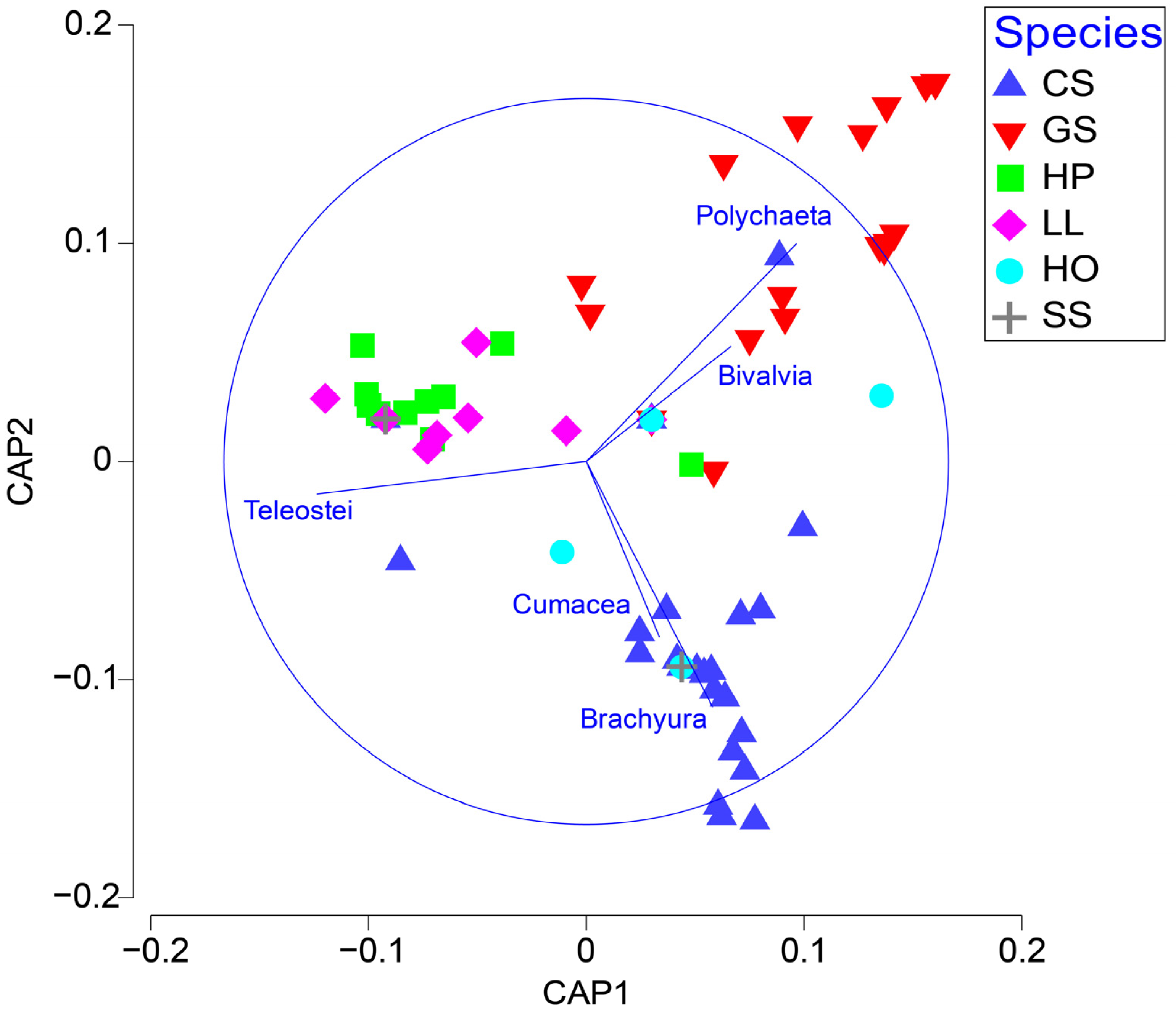
A canonical analysis of the principal coordinates further showed factors that indicated group separation among the six fish species. Teleosts were key in separating C. pinetorum and L. litulon from other species, whereas strong contributions of polychaetes and crabs were observed in the dietary samples of G. stelleri and C. spinosus, respectively. Consequently, the six fish species could be classified into three groups: the first group included piscivorous C. pinetorum, L. litulon, and S. schlegelii; the second group included G. stelleri, which primarily consumed polychaetes; and the last group contained C. spinosus and H. otakii, which mainly ingested crabs (Figure 2).
3.2. Stable Isotope Values
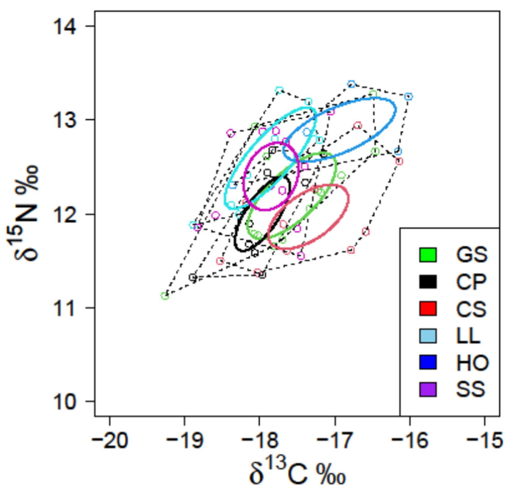
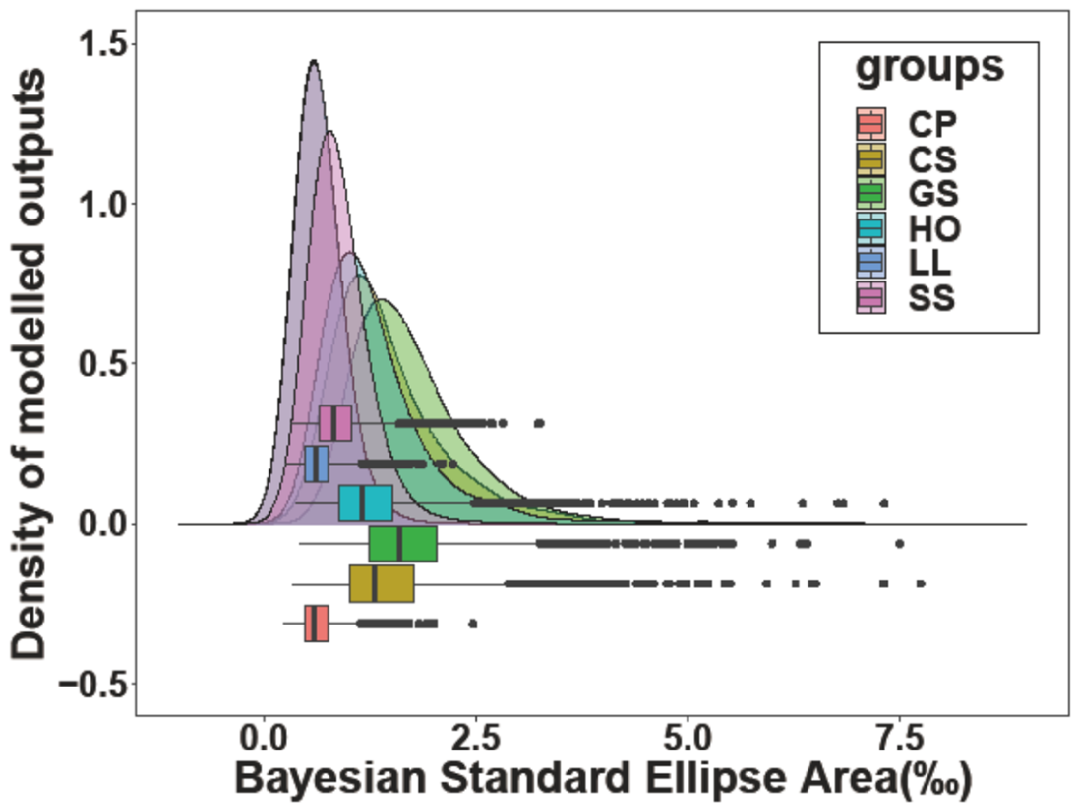
A total of 66 white muscle tissues (16 for C. pinetorum, 10 for C. spinosus, 13 for G. stelleri, 5 for H. otakii, 10 for L. litulon, and 12 for S. schlegelii) were analyzed. The range of δ13C was from −19.529‰ to −16.015‰, and δ15N ranged from 10.670‰ to 13.381‰. The highest mean δ13C (−16.936‰) and δ15N (12.895‰) values were observed in the muscle tissue of H. otakii, whereas the lowest mean values (−18.218‰ in δ13C and 11.737‰ in δ15N) were observed in C. pinetorum (Figure 3). There were significant differences in both δ13C and δ15N values between the six fish species (ANOVA, p < 0.05, F-value = 2.434 for δ13C and 3.625 for δ15N). Tukey’s post hoc tests indicated that the mean δ13C value of H. otakii was higher than those of C. pinetorum, L. litulon, and S. schlegelii, whereas the mean δ15N value of C. pinetorum was lower than those of H. otakii, L. litulon, and S. schlegelii (Tukey’s HSD test, p < 0.05). The highest SEAc was shown in G. stelleri, whereas C. pinetorum had the lowest value. There were two patterns of SEAc values for the six species: C. spinosus, G. stelleri, and H. otakii showed relatively higher values, whereas L. litulon, C. pinetorum, and S. schlegelii showed lower values (ANOVA, p < 0.05) (Figure 3; Table 3). The trophic niche areas of the former species were also higher than those of the latter (Figure 4).
3.3. Trophic Position
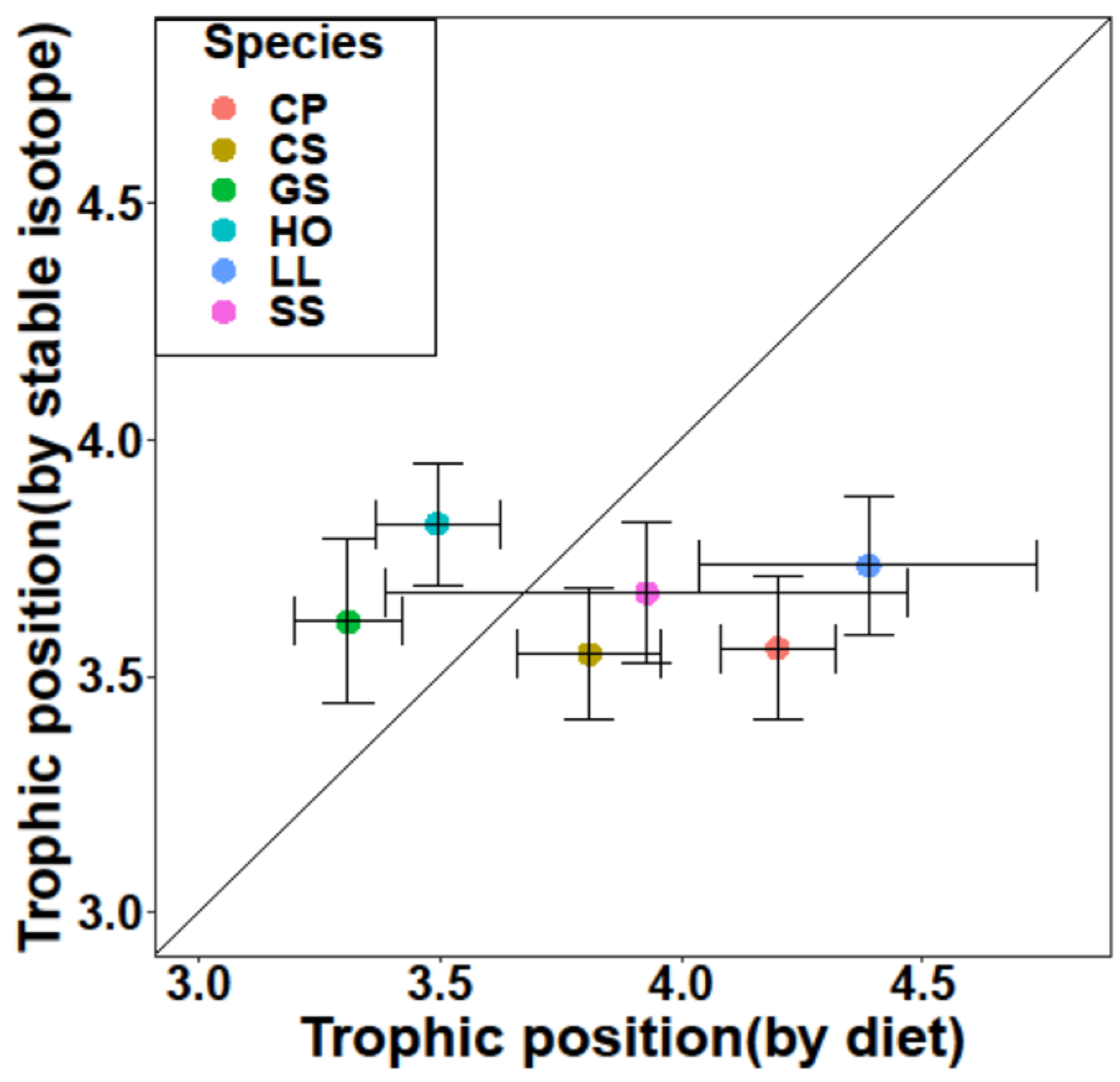
The trophic levels (TROPHs) estimated by stomach content analyses ranged from 3.38 to 4.08, while the values calculated from δ15N ranged from 3.55 to 3.82. The mean TROPH values for C. pinetorum, G. stelleri, H. otakii, and L. litulon were higher than those for the nitrogen (δ15N) stable isotope (ANOVA, p < 0.05), whereas the opposite trends were evident for C. spinosus and S. schlegelii (ANOVA, p > 0.05). In addition, the species with the largest difference in trophic level, calculated by both dietary composition and nitrogen (δ15N) stable isotope value, was L. litulon, located away from the 1:1 line, whereas the smallest gap was observed in S. schlegelii (Figure 5).
4. Discussion
This study demonstrated the food resource uses of six fish species, C. pinetorum, C. spinosus, G. stelleri, H. otakii, L. litulon, and S. schlegelii, which were dominant in terms of abundance during the study period. These species usually inhabit the near-bottom areas of coastal waters. Among the six species, S. schlegelii and H. otakii usually inhabit rocky bottom areas at relatively shallow depths (~30 m), whereas C. spinosus, G. stelleri, C. pinetorum, and L. litulon inhabit relatively deeper waters (normally sandy and/or muddy bottoms) compared to the former two species [21,22]. In our survey of demersal fish assemblage, they were the most common fish species and mainly caught during warm seasons when the period coincided with intensive fishing seasons for flounders and rockfishes. In addition, the six species have been commonly caught in the study area, as well as adjacent coastal waters [23,24,25]. Consequently, this study provided comprehensive analyses of feeding habits of six common fish species using both the SCA and SIA methods.
The results of the dietary analyses for the six species were comparable with those of previous studies undertaken at a larger scale in Korea and adjacent countries. For example, C. spinosus in this study primarily consumed decapod crustaceans (both crabs and carid shrimps) and teleosts secondarily. Similarly, C. spinosus inhabiting the southeastern coast of Korea and around Jeju Island collectively showed high contributions of decapods, including prawns, carid shrimps, and crabs, in the diets [38,39]. The diets of L. litulon in the southern part of the eastern Korean Sea, including the current study area, contained a high proportion of teleosts [40] and is thus regarded as a piscivorous fish. Broad-scale dietary studies of G. stelleri in the East Sea have shown that the species generally feeds on polychaetes, mollusks, and amphipods [41,42], which was similar to the present results. Several dietary studies of S. schlegelii have shown results consistent with those of the present study, consuming mainly teleosts and decapod crustaceans secondarily [43,44,45,46]. There are slightly different trends in prey choices between the current and previous studies for C. pinetorum and H. otakii [45,46,47,48]. Such differences might be attributed to regional differences in the available prey items and/or relatively small sample numbers to describe the feeding habits of C. pinetorum and H. otakii in this study. Nonetheless, some species such as H. otakii and S. schlegelii have shown considerably small sample sizes due to low catches and relatively high ratio of empty stomach, which seems not to have resulted in describing true dietary habits. Therefore, further studies are needed for those fish species.
Diet diversity showed distinct trends of diverse resource use among the six fish species, with higher values for C. spinosus, G. stelleri, and H. otakii and lower values for L. litulon, C. pinetorum, and S. schlegelii. These results are consistent with the dietary analyses of six species—that is, a higher diet diversity was characteristic of benthic invertebrate feeders (the former three species), while a lower diet diversity was shown in the diets of piscivores (the latter three species) (see Table 2). Based on the results of dietary dissimilarities, overall, the diets of the six fish species did not highly overlap (Table 2 and Figure 2). Prey choices of fish species are determined by the extent of accessibility for available prey resources and/or the ability of predators to select specific prey items according to the feeding strategy that maximizes the net energy gain [49,50,51]. For instance, among demersal fish species inhabiting the southern continental shelf of the East Sea, four benthic invertebrate feeders showed relatively higher dietary diversity and niche breadth, whereas these values were lower for piscivores and/or decapod feeders, indicating a more diversified diet for the former four fish species [8].
The resource uses of the six fish species were further assessed using stable isotope analyses, which is a complementary method for determining the trophic ecology of fish with the SCA. Stable isotopes can represent trophic sources accumulated in the body of a predator over several months [52]. Generally, fractionations of carbon and nitrogen isotopes are enriched by about <1‰ and 3–4‰ per trophic level, respectively [36,53,54,55,56]. Thus, a food source could be inferred from the δ13C values, whereas δ15N values are used as a predictor of the relative trophic position [36,56]. The δ13C values for the six fish species in this study ranged from −19.529‰ to −16.015‰, while those of δ15N were between 10.670‰ and 13.381‰. According to Kang et al. [37], the average δ13C and δ15N values of POM in offshore sites were −22.1 ± 1.3‰ and 4.3 ± 0.7‰, and those of epilithic microalgae were −18.8 ± 1.8‰ and 6.6 ± 1.1‰ in the eastern Korean peninsula, respectively. Therefore, the six fish species in this study appeared to be associated with benthic food webs, and they were positioned between secondary and tertiary predators.
The trophic niches described by SEAc for C. spinosus, G. stelleri, and H. otakii were relatively higher than those of the other species, indicating a wider Bayesian SEA. The results of higher SEAc may reflect diverse resource uses among the available food resources, which partially corresponds with the results of the diet diversity [57]. For example, the species that showed a wider trophic niche, including C. spinosus, G. stelleri, and H. otakii, showed a relatively high diet diversity based on the results of the SCA. The range of δ13C and δ15N values in a consumer generally indicates the diversity of trophic resources and positions [58]. In addition, by comparing the results of diet diversity and SEAc results, there can be two types of resource uses, one with a wider trophic niche width and higher diet diversity and the other with a narrow trophic niche width and lower diet diversity.
In terms of trophic levels estimated by both the SCA and SIA, four fish species, C. pinetorum, G. stelleri, H. otakii, and L. litulon, showed significant differences between the two results, with consistently higher TROPH values than isotopic trophic levels. These dissimilarities often occur because of the different temporal resolutions of the two methods. Since SCA identifies the prey that are recently consumed and diverse species and SIA provides assimilated information of prey items for fish species, difference between the trophic levels estimated based on the analyses can generally occur [59,60,61,62].
In this study, differences in resource uses were observed among the six fish species based on the SCA and SIA. There were two types of resource uses for the six fish species: one included three fish species (C. spinosus, G. stelleri, and H. otakii) showing a higher consumption of benthic decapods and/or polychaetes, high diet diversity, and wider trophic niche widths, whereas the other three piscivores showed a relatively lower diet diversity and narrow trophic niche widths. Several studies have described the trophic ecology of fish species using both the SCA and SIA. For example, the three herbivorous Mediterranean fishes showed different trophic positions, especially in terms of the δ15N values, but also indicated differences in prey choices among the taxa of benthic algae [62]. In the fish assemblage from the Western English Channel, although the SIA results reflected a high overlap of trophic niches among fish species, the SCA results indicated that their respective prey items were distinctly segregated [63]. The SCA and SIA did not always produce similar results due to different temporal resolutions [4], but the current study showed consistent trends of resource uses among the six species based on the two analyses. If the available food resources in the habitats are continuously maintained and the patterns of prey choice of the fish species are constant, the SCA and SIA will yield similar results in describing fish dietary habitats. Nevertheless, because the assimilation time of stable isotopes in the fish body is still unclear [64], there has been a limitation in understanding whether prey consumption in a short period of time accurately reflects the fish body due to the accumulation of stable isotopes over a long period.
In conclusion, we analyzed the prey resource utilization of six fish species usually caught in the East Sea off the southern Korean coast by using both the SCA and SIA. The results from this study effectively demonstrated the feeding relationships among the six fish species cooccurring in the study area. In addition, the SCA and SIA methodologies provided the extent of the resource uses for different prey resources among six fish species. Although the lack of sample numbers in this study limits our ability to describe the absolute diets of these species, analyses of the dietary habits and trophic ecology among these fish species are necessary to understand the biological relationships of benthic ecosystems in the southeastern waters of Korea. Overall, our results contribute to the understanding of trophic relationships among fish species inhabiting the East Sea, Korea.
Supplementary Materials
The following supporting information can be downloaded at: https://www.mdpi.com/article/10.3390/w15061146/s1: Table S1: Frequency of occurrence (F) and numerical (N) and mass (M) percentages of prey organisms in the diets of six demersal fish species in the southeastern coast of East Sea, Korea (Species codes: CS, Chelidonichthys spinosus; LL, Lophius litulon; GS, Glyptocephalus stelleri; CP, Cleisthenes pinetorum; HO, Hexagrammos otakii; and SS, Sebastes schlegelii).
Author Contributions
M.-G.K., methodology, validation, formal analysis, investigation, resources, data curation, original draft preparation, and visualization; S.-H.L., supervision and writing—review and editing; M.-J.K. and S.-N.K., investigation and formal analysis; I.-S.H., project administration and funding acquisition; J.-M.P., conceptualization, methodology, validation, formal analysis, and writing—review and editing. All authors have read and agreed to the published version of the manuscript.
Funding
This research was supported by the National Research Foundation of Korea (NRF) grant funded by the Korean government (MSIT) (No. 2020R1F1A1051773). This work was also supported by a project of the Korea Institute of Ocean Science & Technology (grant number: PEA0116). Research support for SHL was provided by the Korea Institute of Marine Science & Technology Promotion (KIMST) funded by the Ministry of Oceans and Fisheries, Korea (20220541).
Data Availability Statement
The data presented in this study are available on request from the corresponding author.
Conflicts of Interest
The authors declare no conflict of interest.
References
- Hussey, N.E.; MacNeil, M.A.; McMeans, B.C.; Olin, J.A.; Dudley, S.F.J.; Cliff, G.; Wintner, S.P.; Fennessy, S.T.; Fisk, A.T. Rescaling the trophic structure of marine food webs. Ecol. Lett. 2014, 17, 239–250. [Google Scholar] [CrossRef] [PubMed]
- Froese, R.; Pauly., D. (Eds.) Fishbase; World Wide Web Electronic Publication. [Version 02/2022]; Available online: http://www.fishbase.org (accessed on 24 October 2022).
- Zanden, M.J.V.; Rasmussen, J.B. Variation in δ15N and δ13C trophic fractionation: Implications for aquatic food web studies. Limnol. Oceanogr. 2001, 46, 2061–2066. [Google Scholar] [CrossRef]
- Park, J.M.; Gaston, T.F.; Williamson, J.E. Resource partitioning in gurnard species using trophic analyses: The importance of temporal resolution. Fish. Res. 2017, 186, 301–310. [Google Scholar] [CrossRef]
- Amundsen, P.A.; Sánchez-Hernández, J. Feeding studies take guts–critical review and recommendations of methods for stomach contents analysis in fish. J. Fish Biol. 2019, 95, 1364–1373. [Google Scholar] [CrossRef] [Green Version]
- Wang, S.; Tang, J.-P.; Su, L.-H.; Fan, J.-J.; Chang, H.-Y.; Wang, T.-T.; Wang, L.; Lin, H.-J.; Yang, Y. Fish feeding groups, food selectivity, and diet shifts associated with environmental factors and prey availability along a large subtropical river, China. Aquat. Sci. 2019, 81, 31. [Google Scholar] [CrossRef]
- Manko, P. Stomach Content Analysis in Freshwater Fish Feeding Ecology; University of Prešov; Prešov, Slovakia, 2016; Volume 116, p. 114. [Google Scholar]
- Park, J.M.; Kwak, S.N.; Huh, S.-H.; Han, I.-S. Diets and niche overlap among nine co-occurring demersal fishes in the southern continental shelf of East/Japan Sea, Korea. Deep Sea Res. Part II Top. Stud. Oceanogr. 2017, 143, 100–109. [Google Scholar] [CrossRef]
- Park, J.M.; Huh, S.-H. Dietary habits and feeding strategy of the fivespot flounder, Pseudorhombus pentophthalmus in the southeastern coast of Korea. Ichthyol. Res. 2017, 64, 93–103. [Google Scholar] [CrossRef]
- Cortés, E. A critical review of methods of studying fish feeding based on analysis of stomach contents: Application to elasmobranch fishes. Can. J. Fish. Aquat. Sci. 1997, 54, 726–738. [Google Scholar] [CrossRef]
- Bearhop, S.; Adams, C.E.; Waldron, S.; Fuller, R.A.; MacLeod, H. Determining trophic niche width: A novel approach using stable isotope analysis. J. Anim. Ecol. 2004, 73, 1007–1012. [Google Scholar] [CrossRef] [Green Version]
- Lin, H.-J.; Kao, W.-Y.; Wang, Y.-T. Analyses of stomach contents and stable isotopes reveal food sources of estuarine detritivorous fish in tropical/subtropical Taiwan. Estuar. Coast. Shelf Sci. 2007, 73, 527–537. [Google Scholar] [CrossRef]
- Cresson, P.; Ruitton, S.; Ourgaud, M.; Harmelin-Vivien, M. Contrasting perception of fish trophic level from stomach content and stable isotope analyses: A Mediterranean artificial reef experience. J. Exp. Mar. Biol. Ecol. 2014, 452, 54–62. [Google Scholar] [CrossRef] [Green Version]
- Knickle, D.C.; Rose, G.A. Dietary niche partitioning in sympatric gadid species in coastal Newfoundland: Evidence from stomachs and CN isotopes. Environ. Biol. Fishes 2014, 97, 343–355. [Google Scholar] [CrossRef]
- Gibson, R.; Ezzi, I. Feeding relationships of a demersal fish assemblage on the west coast of Scotland. J. Fish Biol. 1987, 31, 55–69. [Google Scholar] [CrossRef]
- Fuita, T.; Kitagawa, D.; Okuyama, Y.; Ishito, Y.; Inada, T.; Jin, Y. Diets of the demersal fishes on the shelf off Iwate, northern Japan. Mar. Biol. 1995, 123, 219–233. [Google Scholar] [CrossRef]
- Labropoulou, M.; Papadopoulou-Smith, K.-N. Foraging behaviour patterns of four sympatric demersal fishes. Estuar. Coast. Shelf Sci. 1999, 49, 99–108. [Google Scholar] [CrossRef]
- Madurell, T.; Cartes, J.E. Trophic relationships and food consumption of slope dwelling macrourids from the bathyal Ionian Sea (eastern Mediterranean). Mar. Biol. 2006, 148, 1325–1338. [Google Scholar] [CrossRef]
- De la Morinière, E.C.; Pollux, B.; Nagelkerken, I.; Hemminga, M.; Huiskes, A.; van der Velde, G. Ontogenetic dietary changes of coral reef fishes in the mangrove-seagrass-reef continuum: Stable isotopes and gut-content analysis. Mar. Ecol. Prog. Ser. 2003, 246, 279–289. [Google Scholar] [CrossRef] [Green Version]
- Dromard, C.R.; Bouchon-Navaro, Y.; Harmelin-Vivien, M.; Bouchon, C. Diversity of trophic niches among herbivorous fishes on a Caribbean reef (Guadeloupe, Lesser Antilles), evidenced by stable isotope and gut content analyses. J. Sea Res. 2015, 95, 124–131. [Google Scholar] [CrossRef]
- Yamada, U.; Shirai, S.; Irie, T. Names and Illustrations of Fishes from the East China Sea and the Yellow Sea: Japanese Chinese Korean; Overseas Fishery Cooperation Foundation: Tokyo, Japan, 1995; p. 288. [Google Scholar]
- Ryu, J.H.; Kim, P.-K.; Kim, J.K.; Kim, H.J. Seasonal variation of species composition of fishes collected by gill net and set net in the middle East Sea of Korea. Korean J. Ichthyol. 2005, 17, 279–286. [Google Scholar]
- Hong, B.-K.; Kim, J.-K.; Park, K.-D.; Jeon, K.-A.; Chun, Y.-Y.; Hwang, K.-e.; Kim, Y.-S.; Park, K.-Y. Species composition of fish collected in gill nets from Youngil Bay, East Sea of Korea. Korean J. Fish. Aquat. Sci. 2008, 41, 353–362. [Google Scholar] [CrossRef] [Green Version]
- Choi, J.H.; Kim, J.Y.; Kim, J.K.; Kim, J.B. Seasonal variation of species composition of fish in the coastal waters off Wolseong Nuclear Power Plant, East Sea of Korea by otter trawl survey. Korean J. Fish. Aquat. Sci. 2014, 47, 645–653. [Google Scholar] [CrossRef] [Green Version]
- Seong, G.C.; Ko, A.; Nam, K.M.; Jeong, J.M.; Kim, J.N.; Baeck, G.W. Diet of the Korean flounder Glyptocephalus stelleri in the coastal waters of the east sea of Korea. Korean J. Fish. Aquat. Sci. 2019, 52, 430–436. [Google Scholar] [CrossRef]
- Hyslop, E. Stomach contents analysis—A review of methods and their application. J. Fish Biol. 1980, 17, 411–429. [Google Scholar] [CrossRef] [Green Version]
- Da Silveira, E.L.; Semmar, N.; Cartes, J.E.; Tuset, V.M.; Lombarte, A.; Ballester, E.L.C.; Vaz-dos-Santos, A.M. Methods for Trophic Ecology Assessment in Fishes: A Critical Review of Stomach Analyses. Rev. Fish. Sci. Aquac. 2020, 28, 71–106. [Google Scholar] [CrossRef]
- Warwick, R.M. Environmental impact studies on marine communities: Pragmatical considerations. Aust. J. Ecol. 1993, 18, 63–80. [Google Scholar] [CrossRef]
- Clarke, K.; Gorley, R. Getting Started with PRIMER v7; PRIMER-E; Plymouth Marine Laboratory: Plymouth, UK, 2015; Volume 20, p. 18. [Google Scholar]
- Krebs, C.J. Ecological Methodology; Jarper & Row Publishers: New York, NY, USA, 1989. [Google Scholar]
- Peterson, B.J.; Fry, B. Stable isotopes in ecosystem studies. Annu. Rev. Ecol. Syst. 1987, 18, 293–320. [Google Scholar] [CrossRef]
- Jackson, A.L.; Inger, R.; Parnell, A.C.; Bearhop, S. Comparing isotopic niche widths among and within communities: SIBER—Stable Isotope Bayesian Ellipses in R. J. Anim. Ecol. 2011, 80, 595–602. [Google Scholar] [CrossRef]
- Syväranta, J.; Lensu, A.; Marjomäki, T.J.; Oksanen, S.; Jones, R.I. An empirical evaluation of the utility of convex hull and standard ellipse areas for assessing population niche widths from stable isotope data. PLoS ONE 2013, 8, e56094. [Google Scholar] [CrossRef] [Green Version]
- Pauly, D.; Froese, R.; Sa-a, P.; Palomares, M.; Christensen, V.; Rius, J. TrophLab Manual; Iclarm: Manila, Philippines, 2000. [Google Scholar]
- Pauly, D.; Froese, R.; Palomares, M.L. Fishing down aquatic food webs: Industrial fishing over the past half-century has noticeably depleted the topmost links in aquatic food chains. Am. Sci. 2000, 88, 46–51. [Google Scholar] [CrossRef]
- Post, D.M. Using stable isotopes to estimate trophic position: Models, methods, and assumptions. Ecology 2002, 83, 703–718. [Google Scholar] [CrossRef]
- Kang, C.-K.; Choy, E.J.; Son, Y.; Lee, J.-Y.; Kim, J.K.; Kim, Y.; Lee, K.-S. Food web structure of a restored macroalgal bed in the eastern Korean peninsula determined by C and N stable isotope analyses. Mar. Biol. 2008, 153, 1181–1198. [Google Scholar] [CrossRef]
- Huh, S.-H.; Park, J.M.; Baeck, G.W. Feeding habits of bluefin searobin (Chelidonichthys spinosus) in the coastal waters off Busan. Korean J. Ichthyol. 2007, 19, 51–56. [Google Scholar]
- Kim, J.-B.; Kim, J.-Y.; Lee, D.-W.; Choi, J.-H. Feeding Habits of Bluefin Searobin Chelidonichthys spinosus around Jeju Island. Korean J. Fish. Aquat. Sci. 2011, 44, 378–382. [Google Scholar] [CrossRef]
- Park, J.; Huh, S.H.; Jeong, J.; Baeck, G. Diet composition and feeding strategy of yellow goosefish, Lophius litulon (Jordan, 1902), on the southeastern coast of Korea. J. Appl. Ichthyol. 2014, 30, 151–155. [Google Scholar] [CrossRef]
- Pushchina, O. Specific features of feeding of the Glyptocephalus stelleri and Acanthopsetta nadeshnyi in the northwestern Sea of Japan. J. Ichthyol. 2000, 40, 247–252. [Google Scholar]
- Tokranov, A. Specific features of distribution and some features of biology of Korean flounder Glyptocephalus stelleri (Pleuronectidae) in waters off Kamchatka in the Sea of Okhotsk. J. Ichthyol. 2008, 48, 759–769. [Google Scholar] [CrossRef]
- Park, K.-D.; Kang, Y.-J.; Huh, S.-H.; Kwak, S.-N.; Kim, H.-W.; Lee, H.-W. Feeding ecology of Sebastes schlegeli in the Tongyeong marine ranching area. Korean J. Fish. Aquat. Sci. 2007, 40, 308–314. [Google Scholar] [CrossRef] [Green Version]
- Zhang, B.; Li, Z.; Jin, X. Food composition and prey selectivity of Sebastes schlegeli. J. Fish. Sci. China 2014, 21, 134–141. [Google Scholar]
- Zhang, Y.; Xu, Q.; Xu, Q.; Alós, J.; Zhang, H.; Yang, H. Dietary Composition and Trophic Niche Partitioning of Spotty-bellied Greenlings Hexagrammos agrammus, Fat Greenlings H. otakii, Korean Rockfish Sebastes schlegelii, and Japanese Seaperch Lateolabrax japonicus in the Yellow Sea Revealed by Stomach Content Analysis and Stable Isotope Analysis. Mar. Coast. Fish. 2018, 10, 255–268. [Google Scholar]
- Zhang, R.; Liu, H.; Zhang, Q.; Zhang, H.; Zhao, J. Trophic interactions of reef-associated predatory fishes (Hexagrammos otakii and Sebastes schlegelii) in natural and artificial reefs along the coast of North Yellow Sea, China. Sci. Total Environ. 2021, 791, 148250. [Google Scholar] [CrossRef] [PubMed]
- Huh, S.; Baeck, G. Feeding habits of Hippoglossoides pinetorum collected in the coastal waters of Kori, Korea. Korean J. Ichthyol. 2003, 15, 157–161. [Google Scholar]
- Choi, H.C.; Huh, S.-H.; Park, J.M. Size-related and temporal dietary variations of Hexagrammos otakii in the mid-western coast of Korea. Korean J. Ichthyol. 2017, 29, 117–123. [Google Scholar]
- Gerking, S.D. Feeding Ecology of Fish; Academic Press: San Diego, CA, USA, 1994. [Google Scholar]
- Albouy, C.; Guilhaumon, F.; Villéger, S.; Mouchet, M.; Mercier, L.; Culioli, J.; Tomasini, J.; Mouillot, D. Predicting trophic guild and diet overlap from functional traits: Statistics, opportunities and limitations for marine ecology. Mar. Ecol. Prog. Ser. 2011, 436, 17–28. [Google Scholar] [CrossRef] [Green Version]
- Norton, S.F. A functional approach to ecomorphological patterns of feeding in cottid fishes. In Ecomorphology of Fishes; Springer: Berlin/Heidelberg, Germany, 1995; pp. 61–78. [Google Scholar] [CrossRef]
- Fry, B. Stable Isotope Ecology; Springer: Berlin/Heidelberg, Germany, 2006; Volume 521. [Google Scholar]
- DeNiro, M.J.; Epstein, S. Influence of diet on the distribution of carbon isotopes in animals. Geochim. Cosmochim. Acta 1978, 42, 495–506. [Google Scholar] [CrossRef]
- McConnaughey, T.; McRoy, C. Food-web structure and the fractionation of carbon isotopes in the Bering Sea. Mar. Biol. 1979, 53, 257–262. [Google Scholar] [CrossRef]
- Tieszen, L.L.; Boutton, T.W.; Tesdahl, K.G.; Slade, N.A. Fractionation and turnover of stable carbon isotopes in animal tissues: Implications for δ13C analysis of diet. Oecologia 1983, 57, 32–37. [Google Scholar] [CrossRef]
- Fry, B. Food web structure on Georges Bank from stable C, N, and S isotopic compositions. Limnol. Oceanogr. 1988, 33, 1182–1190. [Google Scholar] [CrossRef]
- Rossman, S.; Berens McCabe, E.; Barros, N.B.; Gandhi, H.; Ostrom, P.H.; Stricker, C.A.; Wells, R.S. Foraging habits in a generalist predator: Sex and age influence habitat selection and resource use among bottlenose dolphins (Tursiops truncatus). Mar. Mammal Sci. 2015, 31, 155–168. [Google Scholar] [CrossRef]
- Newsome, S.D.; Martinez del Rio, C.; Bearhop, S.; Phillips, D.L. A niche for isotopic ecology. Front. Ecol. Environ. 2007, 5, 429–436. [Google Scholar] [CrossRef]
- Gearing, J.N. The Study of Diet and Trophic Relationships through Natural Abundance 13C. In Carbon Isotope Techniques; Academic Press: San Diego, CA, USA, 1991; pp. 201–203. [Google Scholar]
- Macdonald, J.S.; Waiwood, K.G.; Green, R.H. Rates of digestion of different prey in Atlantic cod (Gadus morhua), ocean pout (Macrozoarces americanus), winter flounder (Pseudopleuronectes americanus), and American plaice (Hippoglossoides platessoides). Can. J. Fish. Aquat. Sci. 1982, 39, 651–659. [Google Scholar] [CrossRef]
- Polis, G.A.; Strong, D.R. Food web complexity and community dynamics. Am. Nat. 1996, 147, 813–846. [Google Scholar] [CrossRef]
- Azzurro, E.; Fanelli, E.; Mostarda, E.; Catra, M.; Andaloro, F. Resource partitioning among early colonizing Siganus luridus and native herbivorous fish in the Mediterranean: An integrated study based on gut-content analysis and stable isotope signatures. J. Mar. Biol. Assoc. UK 2007, 87, 991–998. [Google Scholar] [CrossRef] [Green Version]
- Sturbois, A.; Cozic, A.; Schaal, G.; Desroy, N.; Riera, P.; Le Pape, O.; Le Mao, P.; Ponsero, A.; Carpentier, A. Stomach content and stable isotope analyses provide complementary insights into the trophic ecology of coastal temperate bentho-demersal assemblages under environmental and anthropogenic pressures. Mar. Environ. Res. 2022, 182, 105770. [Google Scholar] [CrossRef] [PubMed]
- Trueman, C.N.; McGill, R.A.R.; Guyard, P.H. The effect of growth rate on tissue-diet isotopic spacing in rapidly growing animals. An experimental study with Atlantic salmon (Salmo salar). Rapid Commun. Mass Spectrom. 2005, 19, 3239–3247. [Google Scholar] [CrossRef] [PubMed]
Figure 1.
Location of the study area (within boxed area) in the southeastern waters off East Sea, Korea.
Figure 1.
Location of the study area (within boxed area) in the southeastern waters off East Sea, Korea.

Figure 2.
Canonical analysis of principal coordinates (CAP) showing the distribution of six fish species in a multivariate space. This graph indicated that the six fish species had distinct prey items associated with them (Species codes: CS, Chelidonichthys spinosus; LL, Lophius litulon; GS, Glyptocephalus stelleri; CP, Cleisthenes pinetorum; HO, Hexagrammos otakii; and SS, Sebastes schlegelii).

Figure 3.
Carbon (δ13C) and nitrogen (δ15N) stable isotope compositions for six fish species. The solid and dotted lines indicate corrected standard ellipse areas (SEAc) and convex hull total areas (TA) based on their stable isotope values, respectively (Species codes: CS, Chelidonichthys spinosus; LL, Lophius litulon; GS, Glyptocephalus stelleri; CP, Cleisthenes pinetorum; HO, Hexagrammos otakii; and SS, Sebastes schlegelii).

Figure 4.
Bayesian standard ellipse areas showing the trophic niche for six fish species (Species codes: CS, Chelidonichthys spinosus; LL, Lophius litulon; GS, Glyptocephalus stelleri; CP, Cleisthenes pinetorum; HO, Hexagrammos otakii; and SS, Sebastes schlegelii).
Figure 4.
Bayesian standard ellipse areas showing the trophic niche for six fish species (Species codes: CS, Chelidonichthys spinosus; LL, Lophius litulon; GS, Glyptocephalus stelleri; CP, Cleisthenes pinetorum; HO, Hexagrammos otakii; and SS, Sebastes schlegelii).

Figure 5.
Comparison of the mean trophic position (± SD) estimates of the species included in this study, calculated using dietary and δ15N methods.
Figure 5.
Comparison of the mean trophic position (± SD) estimates of the species included in this study, calculated using dietary and δ15N methods.


Table 1.
Number of stomachs analyzed, percentage of empty stomachs, diet diversity, and mass contributions of prey organisms in the diets of six demersal fish species along the southeastern coast of East Sea, Korea (Species codes: CS, Chelidonichthys spinosus; LL, Lophius litulon; GS, Glyptocephalus stelleri; CP, Cleisthenes pinetorum; HO, Hexagrammos otakii; and SS, Sebastes schlegelii).
| Taxa | CS | LL | GS | CP | HO | SS |
|---|---|---|---|---|---|---|
| Number of stomachs analyzed | 62 | 62 | 26 | 28 | 10 | 25 |
| Empty stomachs (%) | 33.3 | 41.9 | 19.2 | 50.0 | 50.0 | 68.0 |
| Diversity (H’) | 2.782 | 1.282 | 2.432 | 1.885 | 1.834 | 1.567 |
| MACRO ALGAE * | 0.10 | 0.36 | ||||
| POLYCHAETA | 0.34 | 37.31 | 13.08 | |||
| MOLLUSCA | ||||||
| Bivalvia | 1.03 | 11.28 | ||||
| Cephalopoda | 0.06 | 5.28 | 15.43 | 15.00 | ||
| CRUSTACEA | ||||||
| Malacostraca | ||||||
| Euphausiacea | 0.03 | |||||
| Stomatopoda | 0.05 | |||||
| Mysidacea | 0.03 | |||||
| Amphipoda | 0.13 | 3.79 | ||||
| Cumacea | 0.04 | |||||
| Decapoda unidentified | 0.77 | |||||
| Caridea | 21.56 | 9.19 | 30.80 | 20.22 | 20.00 | |
| Brachyura | 41.68 | 0.29 | 51.56 | 28.57 | ||
| Thoracica | 1.31 | |||||
| ECHINODERMATA | ||||||
| Crinoidea | ||||||
| CHORDATA | 28.57 | |||||
| Ascidiacea | ||||||
| Teleostei | 32.91 | 8.07 | ||||
| Unidentified material | 85.53 | 64.34 | 42.86 | |||
| Debris | 8.42 |
Note: * Almost Chlorophyta, Rhodophyta, Phaeophyceae.
Table 2.
Summary of results from the similarity of percentages (SIMPER) pairwise tests for differences among the dietary compositions of the six species. The values above the diagonal line indicate the dissimilarity percentages between the six species, and prey categories beneath the diagonal line are the top three dietary items that contribute the dietary differences between species (Species codes: CS, Chelidonichthys spinosus; LL, Lophius litulon; GS, Glyptocephalus stelleri; CP, Cleisthenes pinetorum; HO, Hexagrammos otakii; and SS, Sebastes schlegelii).
| CS | LL | GS | CP | HO | SS | |
| CS | - | 75.06 | 90.21 | 77.72 | 71.01 | 68.72 |
| LL | Teleostei Brachyura Caridea | - | 96.26 | 49.61 | 97.05 | 48.59 |
| GS | Brachyura Caridea Polychaeta | Teleostei Polychaeta Caridea | - | 90.09 | 86.83 | 99.66 |
| CP | Teleostei Brachyura Caridea | Teleostei Caridea Cephalopoda | Teleostei Caridea Polychaeta | - | 92.14 | 67.88 |
| HO | Brachyura Caridea Teleostei | Teleostei Brachyura Caridea | Brachyura Polychaeta Caridea | Teleostei Brachyura Caridea | - | 76.97 |
| SS | Teleostei Brachyura Caridea | Teleostei Brachyura Caridea | Teleostei Brachyura Polychaeta | Teleostei Brachyura Caridea | Teleostei Brachyura Caridea | - |
Table 3.
Standard ellipse area (SEA) and corrected standard ellipse area (SEAc) values of six fish species in the study area (Species codes: CS, Chelidonichthys spinosus; LL, Lophius litulon; GS, Glyptocephalus stelleri; CP, Cleisthenes pinetorum; HO, Hexagrammos otakii; and SS, Sebastes schlegelii).
| CS | LL | GS | CP | HO | SS | |
|---|---|---|---|---|---|---|
| SEA | 1.016 | 0.524 | 1.019 | 0.507 | 1.015 | 0.807 |
| SEAC | 1.109 | 0.589 | 1.147 | 0.571 | 1.353 | 0.887 |
Disclaimer/Publisher’s Note: The statements, opinions and data contained in all publications are solely those of the individual author(s) and contributor(s) and not of MDPI and/or the editor(s). MDPI and/or the editor(s) disclaim responsibility for any injury to people or property resulting from any ideas, methods, instructions or products referred to in the content. |
© 2023 by the authors. Licensee MDPI, Basel, Switzerland. This article is an open access article distributed under the terms and conditions of the Creative Commons Attribution (CC BY) license (https://creativecommons.org/licenses/by/4.0/).
Share and Cite
MDPI and ACS Style
Kang, M.-G.; Lee, S.-H.; Kim, M.-J.; Kwak, S.-N.; Han, I.-S.; Park, J.-M. Resource Use among Six Commercial Fish Species from the South-Eastern Gill Net Fisheries, Korea. Water 2023, 15, 1146. https://doi.org/10.3390/w15061146
AMA Style
Kang M-G, Lee S-H, Kim M-J, Kwak S-N, Han I-S, Park J-M. Resource Use among Six Commercial Fish Species from the South-Eastern Gill Net Fisheries, Korea. Water. 2023; 15(6):1146. https://doi.org/10.3390/w15061146
Chicago/Turabian StyleKang, Min-Gu, Sang-Heon Lee, Myung-Joon Kim, Seok-Nam Kwak, In-Seong Han, and Joo-Myun Park. 2023. "Resource Use among Six Commercial Fish Species from the South-Eastern Gill Net Fisheries, Korea" Water 15, no. 6: 1146. https://doi.org/10.3390/w15061146
Note that from the first issue of 2016, this journal uses article numbers instead of page numbers. See further details here.