
Can Remotely Sensed Snow Disappearance Explain Seasonal Water Supply?
by
 , , and
Kaitlyn Bishay
1,*,
Nels R. Bjarke
1,
Parthkumar Modi
1,
Justin M. Pflug
2,3,4 and
Ben Livneh
1,4 1
Department of Civil, Environmental, and Architectural Engineering, University of Colorado Boulder, Boulder, CO 80309, USA
2
Earth System Science Interdisciplinary Center, University of Maryland, College Park, MD 20742, USA
3
NASA Goddard Space Flight Center Hydrological Sciences Laboratory, Greenbelt, MD 20771, USA
4
Cooperative Institute for Research in Environmental Sciences, University of Colorado Boulder, Boulder, CO 80309, USA
*
Author to whom correspondence should be addressed.
Water 2023, 15(6), 1147; https://doi.org/10.3390/w15061147
Submission received: 21 December 2022
/
Revised: 16 February 2023
/
Accepted: 8 March 2023
/
Published: 15 March 2023
(This article belongs to the Special Issue The Role of Snow in High-Mountain Hydrologic Cycle)
Abstract
:Understanding the relationship between remotely sensed snow disappearance and seasonal water supply may become vital in coming years to supplement limited ground based, in situ measurements of snow in a changing climate. For the period 2001–2019, we investigated the relationship between satellite derived Day of Snow Disappearance (DSD)—the date at which snow has completely disappeared—and the seasonal water supply, i.e., the April—July total streamflow volume, for 15 snow dominated basins across the western U.S. A Monte Carlo framework was applied, using linear regression models to evaluate the predictive skill—defined here as a model’s ability to accurately predict seasonal flow volumes—of varied predictors, including DSD and in situ snow water equivalent (SWE), across a range of spring forecast dates. In all basins there is a statistically significant relationship between mean DSD and seasonal water supply (p ≤ 0.05), with mean DSD explaining roughly half of the variance. Satellite-based model skill improves later in the forecast season, surpassing the skill of in-situ-based (SWE) models in skill in 10 of the 15 basins by the latest forecast date. We found little to no correlation between model error and basin characteristics such as elevation and the ratio of snow water equivalent to total precipitation. Despite a relatively short data record, this exploratory analysis shows promise for improving seasonal water supply prediction, in particular for snow dominated basins lacking in situ observations.
1. Introduction
Across much of the western United States, a substantial amount of total water supply originates as mountain snowpack in the colder, winter months. Especially at higher elevations, many regions are snow dominated, with estimates of up to 70% of runoff originating as snow ablation [1]. This water is vital for power generation, recreation/municipal use, and agriculture [2,3]. As demand for water increases with population growth [4], so does the importance of accurately predicting water supply. However, widely used operational forecast models still struggle to forecast total seasonal snow water supplies, especially in years with anomalous snowpack and under growing uncertainties from future projected changes to climate. This stresses the need to leverage emerging observational data streams, such as remotely sensed snow observations to help improve forecasts in snow-dominated watersheds.
With relatively low summer precipitation, western U.S. water supplies are dependent on water from snow ablation, with streamflow peaking around April, May, June, and July (AMJJ). One major challenge in the skillful prediction of AMJJ total streamflow volume—defined here as seasonal water supply—is the spatially limited network of in situ measurements of SWE and related characteristics, such as incremental precipitation and snow density. Measurements are sparse and preferentially located, often in areas of easy access, which leads them to under sample a variety of terrains while oversampling more accessible elevations. This relatively homogenous snow sampling makes estimates of watershed-scale hydrology difficult, reducing the accuracy of in situ measurements in regions located in the mid-latitudes [5]. New satellite-based geospatial data has allowed for expanded observation of snow, with studies showing a relationship between remotely sensed snow variables and changes in peak SWE [6], as well as with runoff [7,8] and water supply characteristics [9]. In particular, basin DSD was found to explain over half of the variance in peak SWE across basins located in the western U.S. [6] In this study, we seek to isolate remotely sensed snow disappearance information and investigate its utility in skillfully predicting seasonal water supply for 15 basins across the western United States.
As early as 1906, in situ snow observations have been collected to support hydrologic prediction [10]. Snow course data, collected by teams of researchers, include variables such as snow depth and SWE. More modern methods of in situ snow data include daily measurements from Snow Telemetry (SNOTEL) sites, which are monitored by the Natural Resources Conservation Service (NRCS) and were designed to replace snow course measurements. SNOTEL measurements are typically found in high accumulation, high elevation areas, with an approximate station density of one site per 3400 km2 over the western U.S. This, paired with the cost and difficulty of repairs, limits the widespread availability of SNOTEL data. Additionally, sparse spatial coverage implies that predictions based on SNOTEL must implicitly assume a stationary relationship between snow observed at those points relative to basin-wide SWE volume. This assumption has varying utility dependence on the path of winter storm tracks and a non-stationary climate [11]. Conversely, satellites can monitor the presence of snow nearly continuously over the entire landscape. Despite its limitations, SNOTEL data has been vital in the initialization of many models used to predict seasonal water supply. Previous studies have shown a strong relationship exists between peak SWE and flow volume, with lower peak values of SWE corresponding with less runoff in the snow ablation season [12]. In the Sierra Nevada, a 10% decrease in peak SWE led to larger decreases (9% to 22% reduction) in summer minimum streamflow [13], with minimum downstream flows occurring 3–7 days earlier than average annually with each 10% decrease in SWE. A relationship has also been found between the timing of peak SWE and the volume of AMJJ runoff; earlier peak SWE leads to below average AMJJ runoff [14,15]. When considering the response of annual streamflow volume to changing future snow conditions, the expected outcomes may partially depend on which ablation mechanisms dominate; e.g., changes in aridity, water-inputs, or energy-inputs. There is limited consensus on changes in streamflow volume, but greater consensus on how warming-driven changes in snow ablation will drive earlier peak hydrograph timing [16].
In the last few decades, the emergence of satellite-based snow cover data has allowed for new insights into the state of snow in the West. Satellite-based data is spatiotemporally continuous, in contrast to the limited spatial coverage of SNOTEL data. Several satellite snow products exist, including Landsat’s fractional Snow Covered Area (fSCA) dataset [16], the National Snow and Ice Data Center’s Snow Data Assimilation System (SNODAS) [17], and snow cover estimations derived from data procured by NASA’s Moderate Resolution Imaging Spectroradiometer (MODIS). These products have various strengths and weaknesses: for example, Landsat has high spatial resolution (ranging from 15 m to 60 m, depending on spectral band), but is only available every 16 days [18]. On the other hand, SNODAS assimilates satellite data with a physically based model, providing snow estimates at a 1-day temporal resolution, but with a somewhat coarse spatial resolution of 1 km [17]. Finally, MODIS-based approximations of snow cover have a high temporal resolution derived from twice daily observations onboard NASA’s Terra and Aqua satellites, but a 500 m spatial resolution. Furthermore, due to the limitations of remote sensing, these products do not output a direct estimate of SWE. Instead, they can identify the presence of snow, providing useful information on snow timing. Reconstructions of SWE via remotely sensed data can provide spatially distributed estimates of SWE using assumptions about the snowpack energy balance, but are generally limited to be run only after the snowpack has fully ablated and so are generally only valid for retrospective study [19,20,21].
In the western U.S., the Natural Resources Conservation Service (NRCS) have primarily used SNOTEL SWE as a predictor in water supply forecasts [22]. Statistical models, such as those employed by the NRCS, allow for the inclusion of relevant data while minimizing model complexity, although they are less robust in response to shifts in hydrologic conditions. The U.S. National Weather Service (NWS) also uses snowpack measurements to initialize different process-based models used to simulate river flooding and water supply via their River Forecast Centers (RFCs) [23,24,25]. The main benefit of process-based models is the representation of hydrologic processes and mass balance equations applied through time. However, these representations heavily rely on many trainable parameters, generally requiring extensive data availability and computationally expensive parameter identification procedures.
Although a major source of predictability used in water supply forecasting can be attributed to the SNOTEL network, satellite data provides potentially complementary information that may offer unique skill to predictions. Other studies have explored combining in situ and satellite data within computationally demanding physically based models. For example, the combination of MODIS snow-covered area and in situ data was used to estimate daily SWE within the Sierra Nevada and to improve predictions of streamflow and hydrologic models in the Upper Colorado River Basin using physically based models [26,27]. Similarly, the addition of satellite variables such as fSCA to SNOTEL-based measurements of SWE in a linear regression model were found to improve estimates of spatially distributed SWE in the California Sierra Nevada [28]. Previous analyses by Heldmyer et al. 2021 and Yang et al. 2022 used regression models to demonstrate that remotely sensed snow variables —including annually aggregated DSD—which may explain the majority of the variance of peak SWE, which is among the most important variables in predicting seasonal water supply [29,30]. Although many of these relationships have been separately studied, no work to date has sought to quantify the skill of satellite snow disappearance in directly predicting seasonal water flow volume. This paper explores two novel concepts: (1) the relationship between satellite-derived snow timing variables and seasonal water supply, directly exploring the predictive power of this relationship in a computationally inexpensive linear regression model; and (2) locations and time periods where satellite data may support or even exceed the skill of in situ observations in predicting seasonal water supply. As all satellite (DSD, SFF) and in situ (SNOTEL SWE) predictors evaluated in this study provide snapshots of snow conditions in the study basins, the skill that these variables provide is expected to vary over time and space. Working hypotheses include that satellite-derived linear regression models will provide more information about water supply later in the season, as snow ablation occurs, as well as that the strength of this relationship will be positively related to the annual fraction of precipitation that falls as snow (SWE/P).
2. Materials and Methods
A description of relevant data is included in Section 2.1, with an overview of the 15 study basins. We describe the test of the relationship between satellite-observed DSD and seasonal water supply (Section 2.2), followed by the predictive testing of satellite snow timing variables—separately, as well as in conjunction with in situ observations—on a series of forecast dates in Section 2.3. Forecast validation is explained further in Section 2.4.
2.1. Data Description
A total of 15 basins were selected across the western U.S. to span a range of snow-dominated conditions. Multiple screening criteria followed Modi et al., 2022, resulting in the selected basins and their attributes shown in Figure 1 and listed in Table 1. Basin area was constrained between 350 to 2500 km2, with at least one SNOTEL station within the basin boundary or less than 10 km from the basin boundary, with a full record of SNOTEL [31] and USGS-gaged streamflow observations [32] available between water-years 2001 and 2019 [33]. The selected date range was chosen to overlap with snow timing data from Heldmyer et al., 2021, which motivated this work. The resulting basins fell within snow-dominated ecoregions and were also identified as having minimal anthropogenic influence on streamflow as part of metadata from the GAGESII dataset [34]. Following procedures outlined in Heldmyer et al., 2021, DSD values greater than 275 (day of year) were discarded under the assumption that these pixels are permanently snow-covered.
MODIS-derived raster data of satellite snow cover timing for the western U.S. was obtained from Heldmyer et al., 2021, spanning the years of 2001–2019 at a 500 m resolution. They found that applying a 10% fractional snow covered area (fSCA) threshold in obtaining a binary snow cover series from MODIS snow covered area minimized errors in calculating the day of snow disappearance (DSD), reducing some of the uncertainty associated with canopy masking of snow cover. The basin-wide mean DSD—defined here as the “mean DSD”—is a central predictor variable in this analysis and was calculated for all pixels that experienced complete snow ablation (nvalid) during a one-year period. The pixelwise means for all locations within the basin were then averaged to obtain the annual basin-wide mean DSD. From the same pixelwise data, we further calculated the daily snow free fraction, (SFF) or the fraction of a given basin for which snow has ablated by a specific date. This value was calculated with Equation (1), by determining the fraction of pixels which had DSD values less than or equal to the forecast date (nDSD ≤ day) with respect to nvalid. The dates chosen for this analysis began on 1 April and were evaluated biweekly (on 15 April, 1 May, 15 May), ending on 1 June.
Two sources of in situ data were also used: USGS stream gage data, as well as data from the NRCS’ Snow Telemetry (SNOTEL) sites. The stream gage data, initially accessed as an average daily flow rate, was accumulated to a single value of seasonal water supply volume for that year. For each basin, one SNOTEL site was manually selected to represent in situ SWE at a daily timestep, using beginning of day measurements.
2.2. Evaluation of the Relationship between DSD and Seasonal Water Supply
To determine the strength of the linear relationship between satellite variables (DSD and SFF) and seasonal water supply, the correlation between annual mean water supply and mean DSD was calculated under the assumption that each pixel behaves as a spatially discrete snow pillow. The correlations shown in Figure 1 come from the basin-wide mean correlation between the 19 years of DSD data and the annual values of seasonal water supply (AMJJ total flow volume). For each basin, the Pearson’s correlation coefficient (R) was calculated, where basin-wide mean DSD was identified as the independent variable and the aggregated seasonal water supply for each year was identified as the dependent variable in the sample. Similarly, the strength of the relationship between the DSD and seasonal water supply was evaluated via a linear regression, which was chosen to isolate the connection between variables [33]. Model goodness of fit was evaluated and the R2 and p-value of the regression were reported. The null hypothesis for the regression was that the slope of the regression line is equal to zero, or that there is no observable relationship between the two datasets. To better understand the interannual variability in each source of data and how this may affect model skill, the quartile coefficient of dispersion (QCD) was calculated for each basin. Equation (2) shows the calculation of the QCD for a single data source, where Q1 is equal to the 25th percentile of the data, and Q3 is equal to the 75th percentile of the data. This nonparametric metric is a more robust alternative to the coefficient of variation, which is sensitive to outliers.
2.3. Analysis of Predictive Skill
Historically, 1 April has been an important date for water supply forecasting, as SWE is near its maximum annual value [35]. Here, we evaluated the predictive capabilities of linear models on and after this date—on 1 April, 15 April, 1 May, 15 May, and 1 June—to provide an understanding of how the skill of these models depends on seasonal timing of the prediction and additional, post 1 April snow ablation timing information. After 1 April, decreases in SWE increase the portion of the basin with observable snow disappearance, causing an increase in the amount of available DSD information. The remaining dates were chosen to simulate ‘first of month’ water supply forecasts; to increase the granularity of results, mid-month forecast dates were added. Five different linear models were fit to the AMJJ flow data from 2001–2019, with names and relevant input variables defined in Table 2. In each of these cases, the predictand variable is the seasonal water supply in each basin.
For each basin, a Monte Carlo (MC) approach was used to portray the central tendency of the predictions. Following previous studies, which used MC simulations to estimate probabilistic flood hydrographs, 10,000 random MC simulations were utilized. [36,37]. In each iteration, a random split of the 19 years of data partitioned the data into training and testing datasets, with an optimal train: test ratio of √p:1, where p = √Nu, and Nu is equal to the number of unique input rows (in this case, 19) [38]. Using this method, the fraction of data reserved for model validation was approximately 0.32, which is comparable to that retained in other linear regression studies [39]. Using this iterative resampling of yearly data into independent testing and training datasets, we also sought to reduce model overfit.
To resemble the setup of a true forecast, only data that would have been available on or before the corresponding forecast date was considered for each experiment. For example, on 1 April–the 91st day of the year—DSD values larger than 91 meant that snow had not yet disappeared for those grid cells. Therefore, these values were dropped before computing the spatial mean DSD for each year. A similar procedure was used in calculating SFF (in Equation (1)) to ensure that the model was only provided data that was available on or prior to the forecast date. A linear ordinary least squares (OLS) regression via the scikit-learn and statsmodels Python packages [40,41] was used for the model fitting process. Due to the potential for multicollinearity across predictors, models with more than one predictor variable employed a forward stepwise regression approach to determine which independent variables positively contributed to model fit. Previous research has shown that forward stepwise regression rivals the performance of other predictor variable selection frameworks, which seek to reduce model residuals, such as principal components regression or best subsets regression, and performs well when a potential for multicollinearity is present [42]. Forward stepwise OLS regression was validated and trained for each MC simulation on the subset of training years. To select a model with multiple predictor variables, additional predictors must have reduced the residual sum of squares (RSS), or variance in model error, when the multilinear model was fit.
where VAMJJ is the total AMJJ streamflow volume, or seasonal water supply, β1–3 are model coefficients corresponding to mean DSD, SFF, and SNOTEL SWE terms, and β0 is the model error.
2.4. Model Evaluation
For each of the 10,000 MC simulations, model fit and error statistics were calculated for all linear regression models. After each model was fit, the estimated β values were used in conjunction with the reserved testing data to evaluate the model. The intercept, as well as the relative root mean squared error (rRMSE), Pearson’s correlation (R), and percent bias (PBIAS) were reported. These metrics all provide insight into different facets of the model fit. rRMSE, the standard deviation of the model residuals, was chosen to represent the overall model fit, while the PBIAS was chosen as an operational metric determining how accurate the predictions were with respect to total volume, as well as the direction of the errors. After 10,000 iterations, the median scores and interquartile range (IQR) were reported to capture the central tendency and uncertainty associated with each model. This process was repeated for each basin on each of the five forecast dates (1 April, 15 April, 1 May, 15 May, 1 June). Equations (4) and (5) describe the chosen model fit and error statistics:
where ŷ is the observed value of seasonal water supply, VAMJJ, y is the predicted value of VAMJJ for a given model, and n is equal to the number of predicted values.
3. Results
3.1. Evaluating the Relationship between Satellite Variables and Seasonal Water Supply
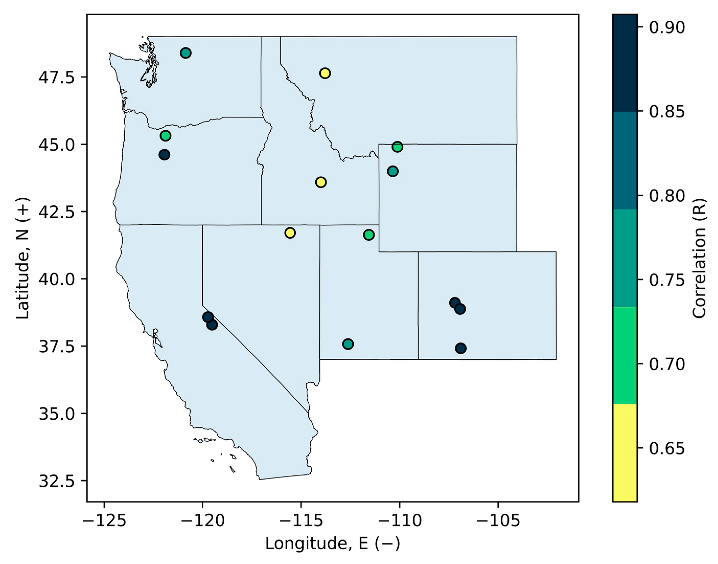
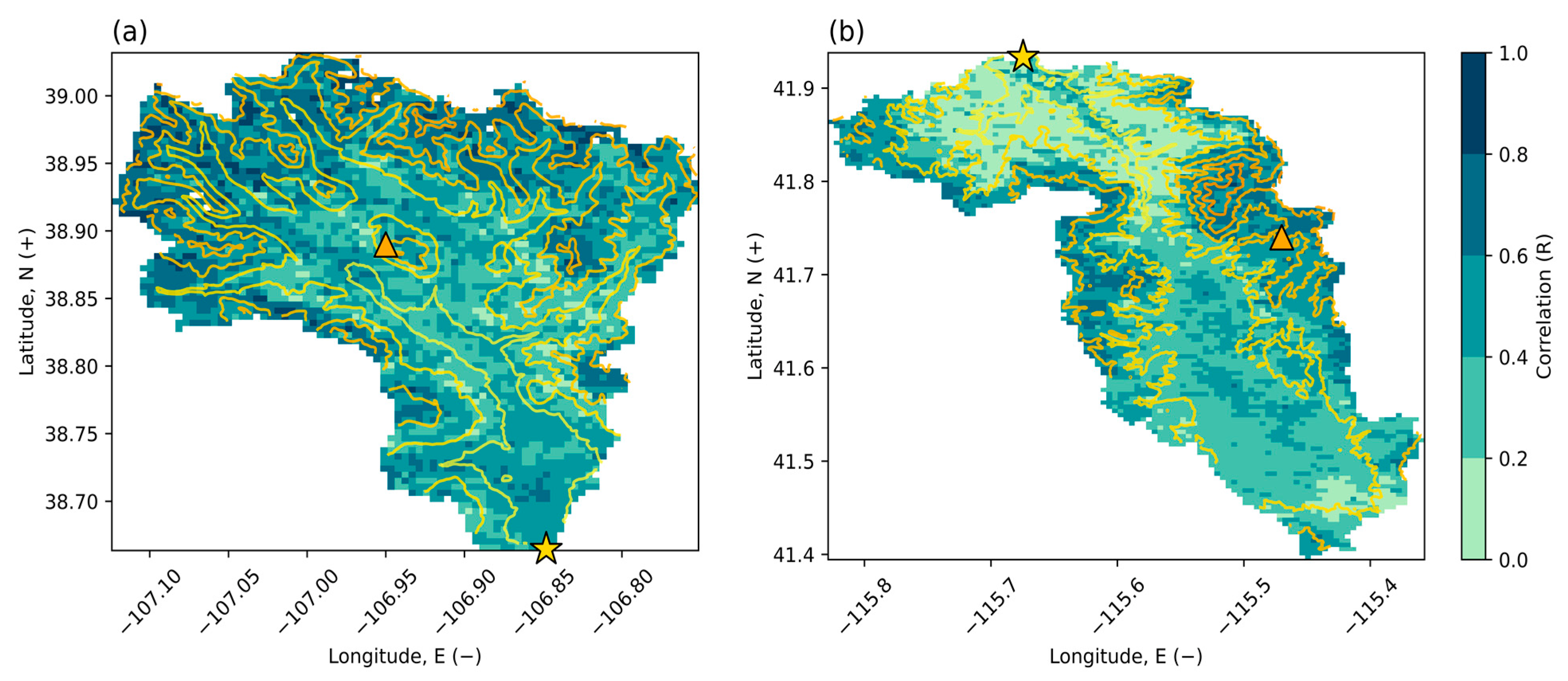
When considering all years of available data, a significant relationship (p ≤ 0.05) exists between DSD and seasonal water supply in all the selected basins. Overall, later DSD values correspond with larger streamflow volume. The associated regression fit statistics are provided in Table 3. Although we focus on basin wide averages, we acknowledge that the correlation between DSD and seasonal water supply spatially varies within each basin, as shown for the East R. basin in Figure 2a—chosen to represent a basin with relatively high overall correlation. Here, as in other basins, we generally see increasing correlation with increasing elevation. In most cases, the selected SNOTEL station is located in a high-elevation portion of the basin where there is a relatively high correlation between the pixelwise DSD and seasonal water supply. These are areas where high snow accumulation is expected. As a result, in situ snow observations at these locations may not be representative of the range of snow conditions found across the entire basin. In basins with lower overall correlation, for instance, the Bruneau R. Basin (Figure 2b), a greater disparity of correlation across the basin can be seen.
While this relationship differs in strength within each basin, approximately half of the yearly variance in seasonal water supply can be explained by the annual mean DSD. The mean correlation for all basins is 0.46 with a median correlation of 0.50. R2 values expected to be larger later in the season, as the DSD information for each year has captured more snow disappearance. Other variables, such as the SFF or SNOTEL SWE, may increase the R2 values within these basins. By discussing the relative predictive skill of each model, the following Sections (Section 3.2 and Section 3.3) discuss how this relationship develops over time and with respect to different predictor variables. The addition of other meteorological predictors—including total precipitation—may improve R2 further but were not considered in this study.
3.2. Evaluation of Forecast Skill of Linear Models Only Using Satellite Data
The predictive strength of the satellite-derived snow information varies throughout the forecasting season. In the case of the example study basin, the East R. (Figure 3), as the season progresses, the satellite-based forecasts improve in rRMSE and R, while PBIAS shows greater variability. When considering overall goodness of fit, we see that the rRMSE consistently decreases during the prediction duration, and correlation between the predicted and observed values rapidly increases until approximately 15 April, where it plateaus and slowly improves. In all cases, model skill generally improves after 1 April, when the proportion of the basin that is snow free increases and provides more descriptive information. In an operational setting, an important metric of the fidelity of water supply models is the PBIAS, which describes the direction and magnitude of errors. In the East R. basin, the Sat_DSD model has a minimum PBIAS when less of the basin is snow covered, with close to zero bias by 15 May. Similarly, the Sat_SFF model is most skillful (−0.071 PBIAS) at the end of the season; when there is more yearly variation in the rate, the basin experiences snow ablation.
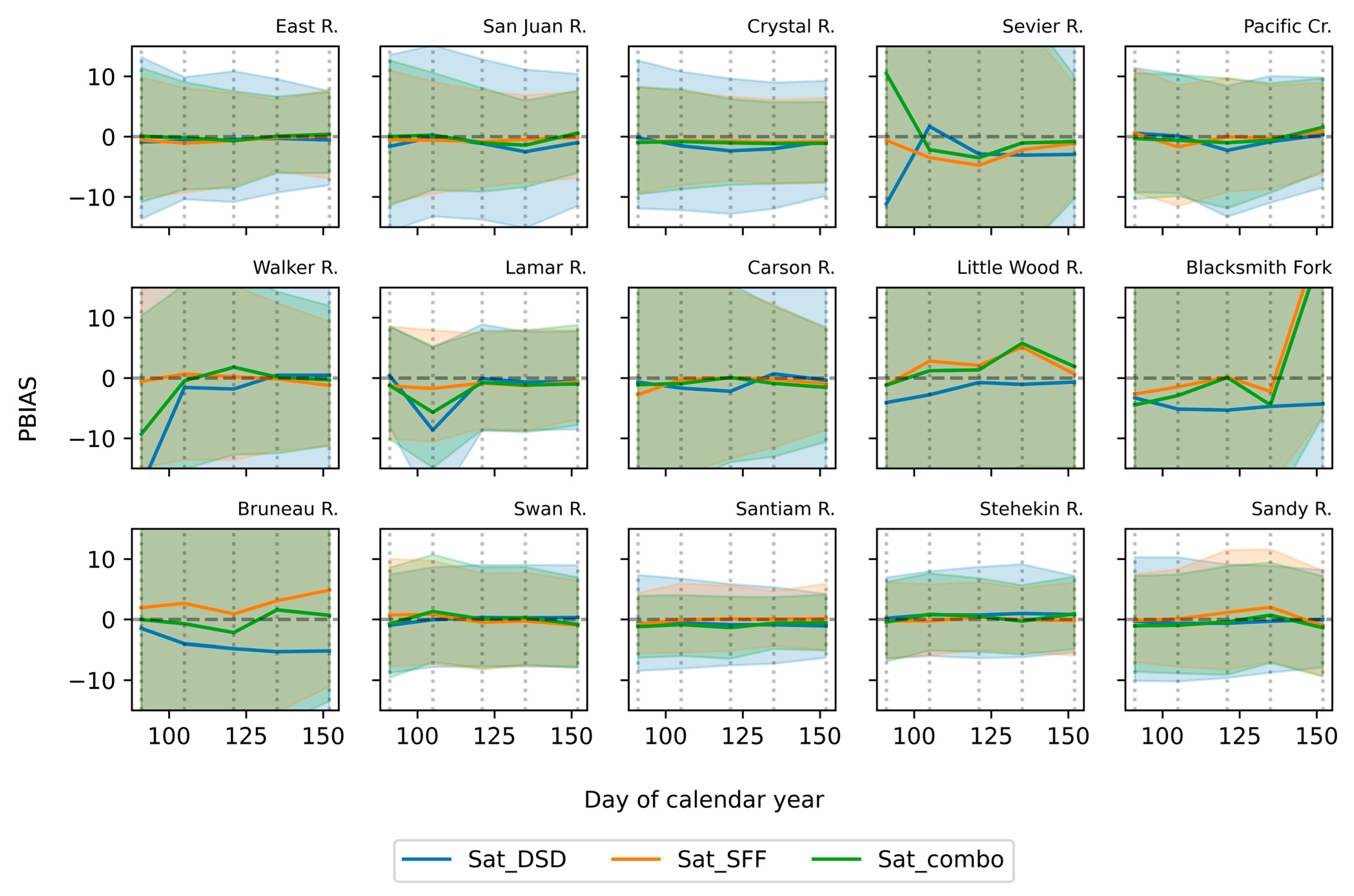
The same generally holds true when considering the other basins. The simplest satellite model (Sat_DSD) has a median 1 April PBIAS of −0.78, whereas the 1 June PBIAS has a median of −0.57. In terms of the overall model fit, the rRMSE varies most substantially from model to model, with a median 1 April rRMSE of 0.33 when considering DSD mean and SFF, and 0.42 only considering DSD mean. In some basins, changes in model skill are not always positive, as can be seen in Figure 4. The addition of additional predictor variables in these basins can increase uncertainty, leading to larger interquartile ranges and small increases in errors in some cases. This can be due to multicollinearity between different predictor variables, which the forward stepwise OLS regression was not able to consistently overcome.
In the San Juan R. basin, in all 10,000 simulations, the RSS for the training set was always reduced when both DSD mean and SFF were introduced as independent variables; i.e., the Sat_combo case. In other basins plotted in Figure 4 (e.g., gages at the Blacksmith Fork and Lamar R. basins), PBIAS is markedly larger in magnitude for the Sat_combo forward stepwise model than other, single variable models. However, in these cases, the “best” model with lowest training RSS was often still the Sat_combo model, using both DSD and SFF information. The increase in absolute PBIAS in these additional basins, despite a low training RSS, suggests large variability within the yearly values of DSD, SFF, and the seasonal water supply. Additional figures for satellite-based model correlation, R, and rRMSE are presented in the Supplementary Materials (Figures S1 and S2, respectively).
3.3. Evaluation of Skill of Linear Models Combining Satellite and In Situ Data
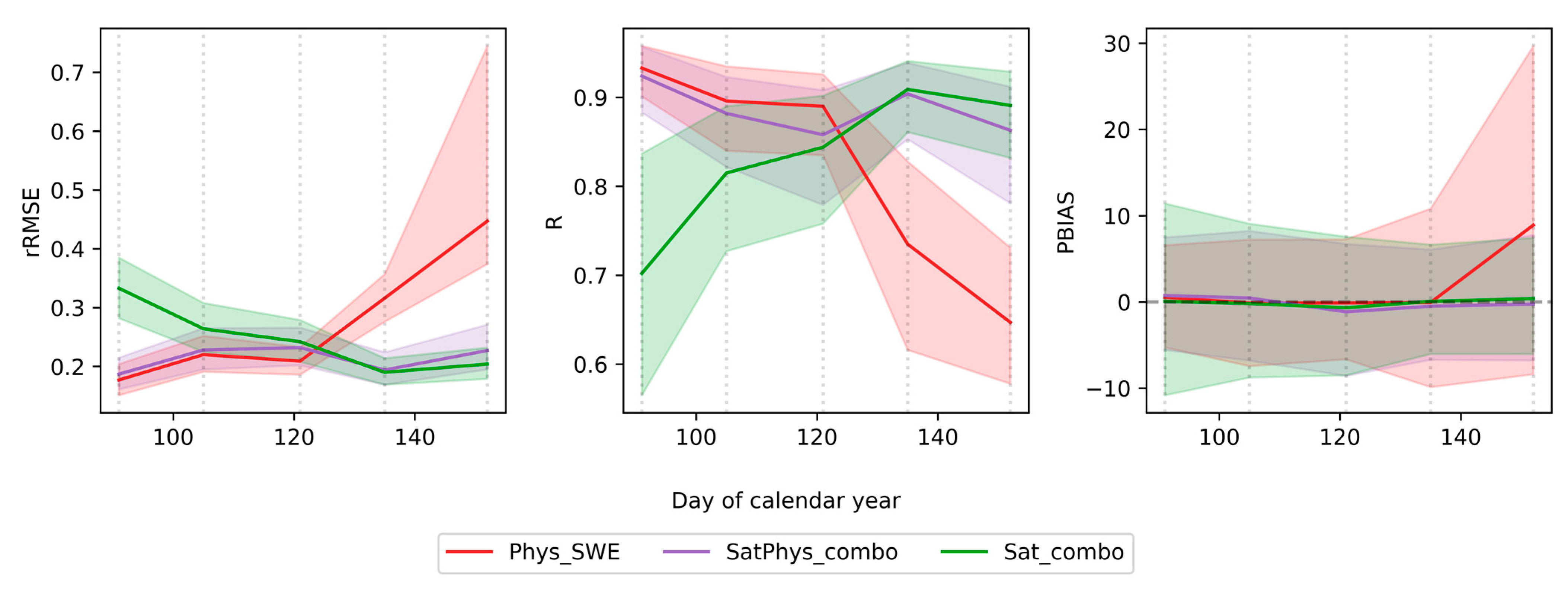
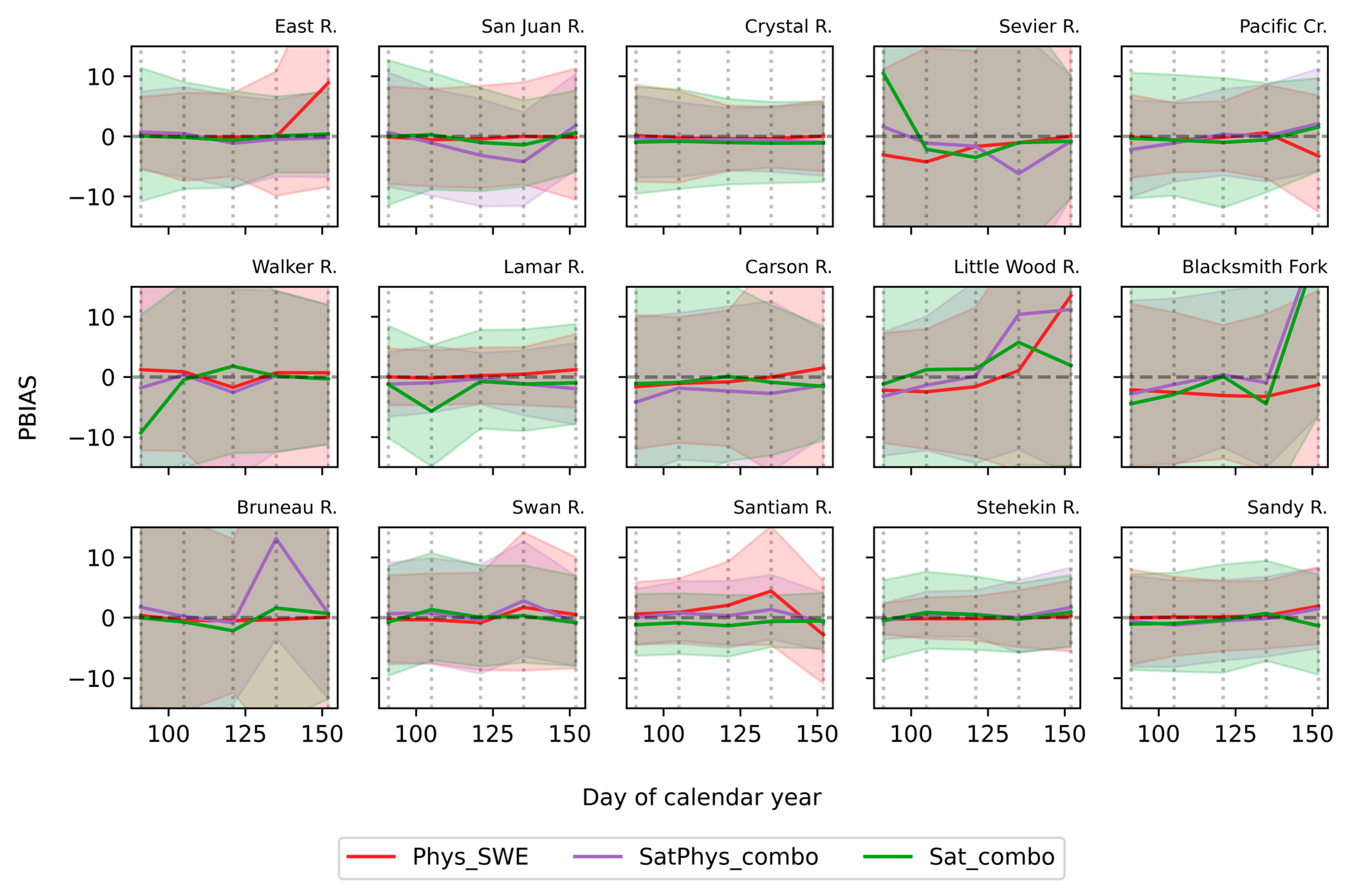
For the East R. gage, the Phys_SWE model outperforms all combinations of the satellite models from 15 April to 15 May with respect to PBIAS (Figure 5). Earlier than 15 April, the Sat_combo model performs best (PBIAS = 0.07), whereas after 15 May, the Sat_SFF model performs best, with a PBIAS of 8.91%. A steep increase in the PBIAS and the magnitude of the IQR, as well as a degradation in skill among other metrics, can be seen in Figure 5. Similarly, by 1 June, the forward stepwise SatPhys_combo model no longer includes SNOTEL SWE as a predictor in every combination, as snow may have ablated at the snow pillow by that time. Throughout the season, the rRMSE improves for the Sat_combo and SatPhys_combo models, but there is a rapid increase in the magnitude of errors for the Phys_SWE model after 1 May. This is consistent with the general phenomenon of correlation increasing in the Sat_combo and SatPhys_combo models across the season, and rapidly decreasing for the Phys_SWE model after 1 May.
When considering the full set of study basins in Figure 6, there is more variability in skill—both in which predictors produce the lowest error, as well as when the best skill is observed in the snow ablation season. For example, in the Blacksmith Fork basin, the Phys_SWE model still produces the least errors in predicting summer flow on 1 June, with the Sat_SFF and Sat_combo models producing significantly more errors. With a basin-wide mean DSD of 104, which is after 1 April, for WY2001–2019, as well as a SWE/P ratio of 0.98, 98% of precipitation in the basin falls as snow, and the satellite models may not capture increased information from DSD and SFF in the Blacksmith Fork basin as the season progresses. However, this pattern is not seen in other basins with low mean DSD, such as the Bruneau R and Sandy R basins, or those with high SWE/P ratios, such as the Pacific Creek and Lamar R basins (SWE/P = 0.96). Additional figures for satellite and in-situ-based model correlation, R, and rRMSE can be found in the Supplementary Materials (Figures S3 and S4, respectively).
4. Discussion
4.1. Insights and Implications
Using satellite snow timing data compiled by Heldmyer et al., 2021 (detailed further in Section 2.1), the relationship between remotely sensed data and seasonal water supply was studied in a range of snow-dominated basins across the western U.S. SNOTEL SWE, a useful predictor in operational water supply forecasts, is spatially limited and unavailable in many basins; consequently, the exploration of MODIS-derived satellite data for prediction of water supply may provide vital information to water managers across the western U.S. Motivated by existing research, this study expanded on previous work that investigated relationships between satellite data and streamflow characteristics, such as peak runoff.
In our attempt to answer whether remotely sensed snow disappearance can explain seasonal water supply variability, a few features appeared. First, due to a lack of snow disappearance at the beginning of the forecast period, the initial hypothesis —that linear models depending on DSD and SFF data improve in their predictive skill over time, as snow disappears—cannot be rejected in most basins. In some basins, such as the East R. and Pacific Cr. basins, PBIAS skill did not consistently improve from 1 April to 1 June. However, the central tendency of other error metrics, such as the rRMSE, did improve over the course of the forecast period. In those same basins, as well as seven others (Walker R., Lamar R., Stehekin R., Carson R., Little Wood R., Santiam R., and Sevier R.) there was at least one instance in which the rRMSE of the Sat_DSD and Sat_combo models increased from one date to the next. In five of the nine basins, which saw increases in rRMSE over time, this decrease came before the date of mean DSD.
Interestingly, a strong correlation exists between basin SWE/P ratio and model error, as shown in Table 4, or between gage elevation and model error, as shown in Table S1. The strength of this result varies when averaged across the forecasting season, but the Phys_SWE model showed the highest correlation between SWE/P ratio and model error, as well as the only relationship that can be described as statistically significant (p ≤ 0.05). The variation associated with DSD and SFF are related to physical processes, which may not be well represented by these metrics. For example, while the DSD may give some indication regarding how wet/warm a water year is, it does not allow for an interpretation of physical processes to explain the separate implications of temperature, solar radiation, and/or deviations from expected meteorological conditions. Similarly, the methods described in this paper assume that seasonal water supply can be represented by changes in snow-covered areas, suggesting that only pixels that have experienced complete ablation will contribute to seasonal water supply. In basins with areas of permanent snowpack, this assumption may introduce a source of error, since permanent snowpacks will contribute some water to melt, but will not be included in the aggregated DSD calculation.
The Sat_DSD and Sat_SFF models varied in predictive skill across basins, as presented in Figure 4. In some basins, DSD was consistently more skillful, or vice versa. This suggests that there may be some combination of basin characteristics (i.e., slope, aspect, or vegetation cover) which were not considered, under which one of these predictor variables is most skillful. When comparing the skill of satellite-based models with those which rely on in situ data, we found that those using in situ observations of SWE (from SNOTEL) may be more informative than remotely sensed estimates of snow disappearance in predicting seasonal water supply. This may be due to greater year-to-year variation in SNOTEL SWE; for each basin in the analysis, the quartile coefficient of dispersion was calculated via Equation (2) and is shown in Figure 7. This coefficient is a proxy for the spread of data; i.e., how wide its distribution is. This variation in yearly SWE is larger than the variation in DSD in every basin, but it becomes less pronounced as the season progresses.
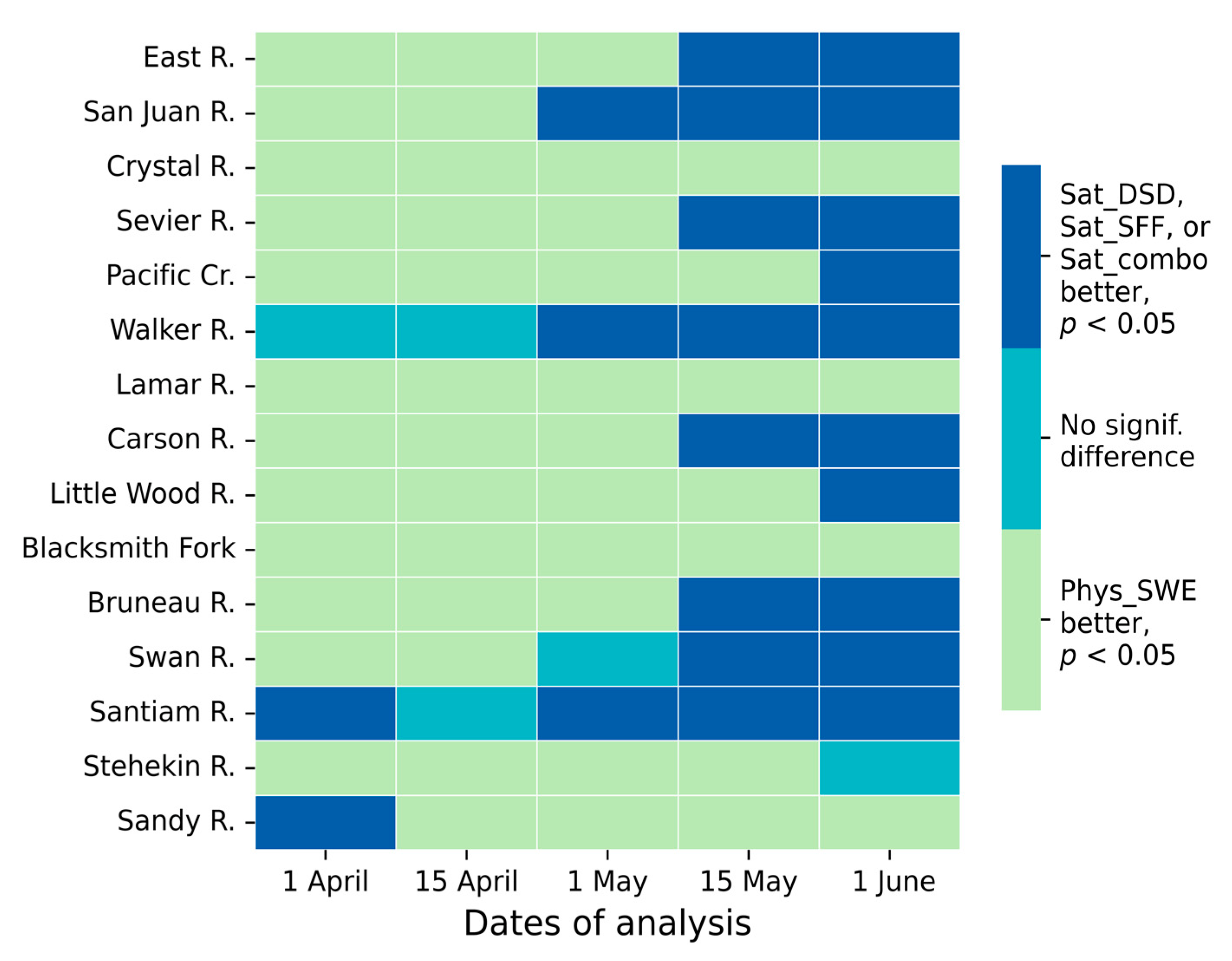
The relative skill of satellite and in situ models also varies with time. Using a Mann-Whitney U Test (also known as a Wilcoxon Rank Sum Test), a nonparametric comparison of model distributions, the distribution of the satellite model predictive metrics with lowest median PBIAS (i.e., Sat_DSD, Sat_SFF, or Sat_combo) was compared to the distribution of the Phys_SWE model, to provide an understanding of when and where the skill is significantly different.
A visualization of the mean difference in absolute PBIAS distribution for all 10,000 iterations is shown in Figure 8. Here, we see that, in many basins, in-situ-based models show higher skill in predicting seasonal water supply than satellite-based models before 1 May. Although the behavior varies by basin, those with high SWE/P ratios tend to see better model skill from SWE-based predictions (Phys_SWE, SatPhys_combo). In the Blacksmith Fork (SWE/P = 0.98) and Lamar R. (SWE/P = 0.96) basins, the skill of the Phys_SWE model is always significantly higher. The opposite is true for basins with low SWE/P ratios, such as the Santiam R. (SWE/P = 0.24) basin, where satellite variables have significantly higher predictive skill for most, if not all, dates analyzed.
Another important perspective on the question posed in this paper is that, given limited SNOTEL coverage across the western U.S., predictive capabilities solely provided by satellite-derived snow information show promise in providing predictive information for less well-served water communities that may not have a SNOTEL station in their basin. Similarly, changes in storm-track and overall climate could potentially imperil the relationship between SWE observed at SNOTEL locations and seasonal water supply, such that remote sensing would be likely to become increasingly important to supplement in situ observations in making predictions in future years.
4.2. Limitations
The availability of DSD data used here was constrained to data obtained and processed by Heldmyer et al., 2021; as a result, each model was only fit on data from 2001–2019 (19 years of available data). This limited sample size restricted the maximum number of predictor variables used in the models to avoid model overfit. In addition, despite efforts towards a large degree of resampling, e.g., 10,000 iterations of model fitting, the short record may still lead to model overfitting as there are fewer training samples for each prediction, as well as an increased possibility for outliers to skew model fit. On a physical level, a key limitation of satellite variables previously mentioned is they do not provide a direct estimate of water volume, rather only an indirect measurement of the timing of snow presence. Moreover, we acknowledge that all variables used in this study (remotely sensed and in situ) are subject to observational errors. In particular, the estimation of snow disappearance from satellite-derived spectral data is an indirect measurement of ‘true’ snow disappearance, expected to introduce additional error to the study. While the errors associated with uncertainties in satellite-derived DSD have been explored with respect to errors in spatially distributed snow reconstructions, the effect of these uncertainties on aggregated data has not been studied [43]. Finally, this analysis has been applied to relatively small basins compared to the larger western U.S., given the availability of unmanaged streamflow and concomitant snow observations. Further investigations into the utility of this methodology applied to larger basins could provide additional insight into the further potential of DSD in forecasting. As the size of the study area of interest increases, the use of a more spatially comprehensive predictor such as DSD could provide unique predictive skill relative to traditional methodologies that rely on sparse in situ observations.
4.3. Future Research Directions
To answer the posed research question(s), this study considered relatively simple linear models to portray general relationships between variables. However, emerging machine learning techniques, which may capture non-linear interactions, as well as models considering a broader suite of predictor variables, could be used in future analyses. As time progresses and the remotely sensed record length grows, the overarching question of this manuscript should be revisited and reanalyzed with updated data records to understand how these trends may change in a future climate and under a broader set of conditions, especially with respect to anomalous years beyond what has already been observed in the historical record.
5. Conclusions
In summary, we revisit the question posed in the title of the paper—can remotely sensed snow disappearance predict seasonal water supply? We can affirmatively answer, with all 15 of the study basins showing a statistically significant (p ≤ 0.05) explanatory relationship between remotely sensed snow variables and seasonal water supply for WY2001–2019. In addition, using satellite-derived snow disappearance information to predict water supply showed notable skill, with a seasonal average of less than 2% bias in linear models (Sat_DSD, Sat_SFF, Sat_combo) in every basin surveyed. This work has broad operational applications across the western U.S., especially in those areas without in situ monitoring sites available.
Supplementary Materials
The following supporting information can be downloaded at: https://www.mdpi.com/article/10.3390/w15061147/s1, Figure S1: The median rRMSE statistics for three different satellite-based water supply forecasts with interquartile range (25/75 percentiles) shaded, for all 15 study basins. Vertical dotted lines denote the days chosen for forecasting—1 April, 15 April, 1 May, 15 May, and 1 June; Figure S2: The median correlation, R, statistics for three different satellite-based water supply forecasts with interquartile range (25/75 percentiles) shaded, for all 15 study basins. Vertical dotted lines denote the days chosen for forecasting—1 April, 15 April, 1 May, 15 May, and 1 June; Figure S3: The median rRMSE statistics for three different satellite and in-situ-based water supply forecasts with interquartile range shaded, for all 15 study basins. Vertical dotted lines denote the days chosen for forecasting—1 April, 15 April, 1 May, 15 May, and 1 June; Figure S4: The median correlation, R, statistics for three different satellite and in-situ-based water supply forecasts with interquartile range shaded, for all 15 study basins. Vertical dotted lines denote the days chosen for forecasting—1 April, 15 April, 1 May, 15 May, and 1 June. Due to a lack of recorded SWE on the forecast dates for any year in the study period, some basins (e.g., Sevier R. and Pacific Cr.) have an undefined correlation coefficient, R, for the Phys_SWE model. This is because Pearson’s correlation coefficient, R, cannot be defined for a constant input array and, after complete snow ablation, SWE is equal to zero for all years studied; Table S1: Correlation between USGS gage elevation and median PBIAS values for all basins calculated for each model and each forecast date. Values with a significant relationship (p-value < 0.05) are marked with an asterisk.
Author Contributions
Conceptualization and methodology, K.B., B.L. and J.M.P.; data curation, N.R.B. and P.M.; writing—original draft preparation, K.B.; writing—review and editing, B.L., J.M.P., P.M. and N.R.B. All authors have read and agreed to the published version of the manuscript.
Funding
This research was supported by the following grants: National Aeronautics and Space Administration: NASA Grant # 80NSSC18K0951: “A Remotely Sensed Ensemble to Understand Human Impacts on the Water Cycle”, USGS Grant # G21AC10645: “Estimation of Future High-Mountain Snowpack to Inform Terrestrial and Aquatic Species Status Assessments, Recovery Plans, and Monitoring”, and NOAA Grant # NA21OAR4310309: “Western Water Assessment: Building Resilience to Compound Hazards in the Inter-Mountain West”.
Data Availability Statement
Maps of remotely sensed snow timing data can be accessed at http://doi.org/10.5281/zenodo.4327643 (accessed on 13 January 2023) [44]. Observational data from the SNOTEL network and USGS gages can be accessed publicly at the references provided in the Section 2.
Conflicts of Interest
The authors declare no conflict of interest.
References
- Li, D.; Wrzesien, M.L.; Durand, M.; Adam, J.; Lettenmaier, D.P. How Much Runoff Originates as Snow in the Western United States, and How Will That Change in the Future? Geophys. Res. Lett. 2017, 44, 6163–6172. [Google Scholar] [CrossRef] [Green Version]
- Schumacher, B.L.; Yost, M.A.; Burchfield, E.K.; Allen, N. Water in the West: Trends, Production Efficiency, and a Call for Open Data. J. Environ. Manag. 2022, 306, 114330. [Google Scholar] [CrossRef] [PubMed]
- Escriva-Bou, A.; McCann, H.; Hanak, E.; Lund, J.; Gray, B.; Blanco, E.; Jezdimirovic, J.; Magnuson-Skeels, B.; Tweet, A. Water Accounting in Western US, Australia, and Spain: Comparative Analysis. J. Water Resour. Plan. Manag. 2020, 146, 04020004. [Google Scholar] [CrossRef]
- Schwabe, K.; Nemati, M.; Landry, C.; Zimmerman, G. Water Markets in the Western United States: Trends and Opportunities. Water 2020, 12, 233. [Google Scholar] [CrossRef] [Green Version]
- Lundquist, J.; Hughes, M.; Gutmann, E.; Kapnick, S. Our Skill in Modeling Mountain Rain and Snow Is Bypassing the Skill of Our Observational Networks. Bull. Am. Meteorol. Soc. 2019, 100, 2473–2490. [Google Scholar] [CrossRef] [Green Version]
- Heldmyer, A.; Livneh, B.; Molotch, N.; Rajagopalan, B. Investigating the Relationship Between Peak Snow-Water Equivalent and Snow Timing Indices in the Western United States and Alaska. Water Resour. Res. 2021, 57, e2020WR029395. [Google Scholar] [CrossRef]
- Kuchment, L.S.; Romanov, P.; Gelfan, A.N.; Demidov, V.N. Use of Satellite-Derived Data for Characterization of Snow Cover and Simulation of Snowmelt Runoff through a Distributed Physically Based Model of Runoff Generation. Hydrol. Earth Syst. Sci. 2010, 14, 339–350. [Google Scholar] [CrossRef] [Green Version]
- Immerzeel, W.W.; Droogers, P.; de Jong, S.M.; Bierkens, M.F.P. Satellite Derived Snow and Runoff Dynamics in the Upper Indus River Basin. Grazer Schr. Geogr. Raumforsch. 2010, 45, 303–312. [Google Scholar]
- Rango, A.; Salomonson, V.V.; Foster, J.L. Seasonal Streamflow Estimation in the Himalayan Region Employing Meteorological Satellite Snow Cover Observations. Water Resour. Res. 1977, 13, 109–112. [Google Scholar] [CrossRef]
- Helms, D.; Phillips, S.E.; Reich, P.F. The History of Snow Survey and Water Supply Forecasting: Interviews with U.S. Department of Agriculture Pioneers; U.S. Department of Agriculture, Natural Resources Conservation Service: Washington, DC, USA, 2008. [Google Scholar]
- Milly, P.C.D.; Betancourt, J.; Falkenmark, M.; Hirsch, R.M.; Kundzewicz, Z.W.; Lettenmaier, D.P.; Stouffer, R.J. Stationarity Is Dead: Whither Water Management? Science 2008, 319, 573–574. [Google Scholar] [CrossRef]
- Dyer, J. Snow Depth and Streamflow Relationships in Large North American Watersheds. J. Geophys. Res. 2008, 113, D18113. [Google Scholar] [CrossRef]
- Godsey, S.E.; Kirchner, J.W.; Tague, C.L. Effects of Changes in Winter Snowpacks on Summer Low Flows: Case Studies in the Sierra Nevada, California, USA. Hydrol. Process. 2014, 28, 5048–5064. [Google Scholar] [CrossRef]
- Dudley, R.W.; Hodgkins, G.A.; McHale, M.R.; Kolian, M.J.; Renard, B. Trends in Snowmelt-Related Streamflow Timing in the Conterminous United States. J. Hydrol. 2017, 547, 208–221. [Google Scholar] [CrossRef] [Green Version]
- Miller, W.P.; Piechota, T.C. Trends in Western U.S. Snowpack and Related Upper Colorado River Basin Streamflow. J. Am. Water Resour. Assoc. 2011, 47, 1197–1210. [Google Scholar] [CrossRef]
- Selkowitz, D.J.; Painter, T.H.; Rittger, K.; Schmidt, G.; Forster, R. The USGS Landsat Snow Covered Area Products: Methods and Preliminary Validation. In Automated Approaches for Snow and Ice Cover Monitoring Using Optical Remote Sensing; University of Utah: Salt Lake City, UT, USA, 2017; pp. 76–119. [Google Scholar]
- National Operational Hydrologic Remote Sensing Center. Snow Data Assimilation System (SNODAS) Data Products at NSIDC, Version 1; National Snow and Ice Data Center: Boulder, CO, USA, 2004. [Google Scholar] [CrossRef]
- Dietz, A.J.; Kuenzer, C.; Gessner, U.; Dech, S. Remote Sensing of Snow—A Review of Available Methods. Int. J. Remote Sens. 2012, 33, 4094–4134. [Google Scholar] [CrossRef]
- Molotch, N.P. Reconstructing Snow Water Equivalent in the Rio Grande Headwaters Using Remotely Sensed Snow Cover Data and a Spatially Distributed Snowmelt Model. Hydrol. Process. 2009, 23, 1076–1089. [Google Scholar] [CrossRef]
- Molotch, N.P.; Margulis, S.A. Estimating the Distribution of Snow Water Equivalent Using Remotely Sensed Snow Cover Data and a Spatially Distributed Snowmelt Model: A Multi-Resolution, Multi-Sensor Comparison. Adv. Water Resour. 2008, 31, 1503–1514. [Google Scholar] [CrossRef]
- Bair, E.H.; Rittger, K.; Davis, R.E.; Painter, T.H.; Dozier, J. Validating Reconstruction of Snow Water Equivalent in California’s Sierra Nevada Using Measurements from the NASAAirborne Snow Observatory: SWE reconstruction compared to ASO. Water Resour. Res. 2016, 52, 8437–8460. [Google Scholar] [CrossRef]
- USDA. Statistical Techniques Used in the VIPER Water Supply Forecasting Software; United States Department of Agriculture: Washington, DC, USA, 2007. [Google Scholar]
- Werner, K.; Brandon, D.; Clark, M.; Gangopadhyay, S. Incorporating Medium-Range Numerical Weather Model Output into the Ensemble Streamflow Prediction System of the National Weather Service. J. Hydrometeorol. 2005, 6, 101–114. [Google Scholar] [CrossRef] [Green Version]
- Day, G.N. Extended Streamflow Forecasting Using NWSRFS. J. Water Resour. Plan. Manag. 1985, 111, 157–170. [Google Scholar] [CrossRef]
- Hamill, T. The national weather service river forecast system. In Proceedings of the 1999 Georgia Water Resources Conference, Athens, GA, USA, 30–31 March 1999. [Google Scholar]
- Guan, B.; Molotch, N.P.; Waliser, D.E.; Jepsen, S.M.; Painter, T.H.; Dozier, J. Snow Water Equivalent in the Sierra Nevada: Blending Snow Sensor Observations with Snowmelt Model Simulations: Snow water equivalent in the Sierra Nevada. Water Resour. Res. 2013, 49, 5029–5046. [Google Scholar] [CrossRef]
- Micheletty, P.; Perrot, D.; Day, G.; Rittger, K. Assimilation of Ground and Satellite Snow Observations in a Distributed Hydrologic Model for Water Supply Forecasting. J. Am. Water Resour. Assoc. 2021, 58, 1030–1048. [Google Scholar] [CrossRef]
- Yang, K.; Musselman, K.N.; Rittger, K.; Margulis, S.A.; Painter, T.H.; Molotch, N.P. Combining Ground-Based and Remotely Sensed Snow Data in a Linear Regression Model for Real-Time Estimation of Snow Water Equivalent. Adv. Water Resour. 2022, 160, 104075. [Google Scholar] [CrossRef]
- Page, R.; Dilling, L. The Critical Role of Communities of Practice and Peer Learning in Scaling Hydroclimatic Information Adoption. Weather Clim. Soc. 2019, 11, 851–862. [Google Scholar] [CrossRef]
- Livneh, B.; Badger, A.M. Drought Less Predictable under Declining Future Snowpack. Nat. Clim. Change 2020, 10, 452–458. [Google Scholar] [CrossRef]
- USDA Natural Resources Conservation Service. SNOwpack TELemetry Network (SNOTEL); Natural Resources Conservation Service—NRCS: Washington, DC, USA, 2022. [Google Scholar]
- US Geological Survey. USGS Water Data for the Nation; US Geological Survey: Washington, DC, USA, 1994. [Google Scholar] [CrossRef]
- Modi, P.A.; Small, E.E.; Kasprzyk, J.; Livneh, B. Investigating the Role of Snow Water Equivalent on Streamflow Predictability during Drought. J. Hydrometeorol. 2022, 23, 1607–1625. [Google Scholar] [CrossRef]
- US Geological Survey. GAGES-II: Geospatial Attributes of Gages for Evaluating Streamflow; US Geological Survey: Washington, DC, USA, 2011. [Google Scholar]
- Cayan, D.R. Interannual Climate Variability and Snowpack in the Western United States. J. Clim. 1996, 9, 928–948. [Google Scholar] [CrossRef]
- Loveridge, M.; Rahman, A.; Babister, M. Probabilistic Flood Hydrographs Using Monte Carlo Simulation: Potential Impact to Flood Inundation Mapping. In Proceedings of the MODSIM2013, 20th International Congress on Modelling and Simulation, Adelaide, Australia, 1–6 December 2013; Piantadosi, J., Anderssen, R.S., Boland, J., Eds.; Modelling and Simulation Society of Australia and New Zealand (MSSANZ), Inc.: Canberra, Australia, 2013. [Google Scholar]
- Charalambous, J.; Rahman, A.; Carroll, D. Application of Monte Carlo Simulation Technique to Design Flood Estimation: A Case Study for North Johnstone River in Queensland, Australia. Water Resour. Manag. 2013, 27, 4099–4111. [Google Scholar] [CrossRef]
- Joseph, V.R. Optimal Ratio for Data Splitting. Stat. Anal. Data Min. ASA Data Sci. J. 2022, 15, 531–538. [Google Scholar] [CrossRef]
- Kommineni, M.; Reddy, K.V.; Jagathi, K.; Reddy, B.D.; Roshini, A.; Bhavani, V. Groundwater Level Prediction Using Modified Linear Regression. In Proceedings of the 2020 6th International Conference on Advanced Computing and Communication Systems (ICACCS), Coimbatore, India, 6–7 March 2020; IEEE: Coimbatore, India, March, 2020; pp. 1164–1168. [Google Scholar]
- Pedregosa, F.; Varoquaux, G.; Gramfort, A.; Michel, V.; Thirion, B.; Grisel, O.; Blondel, M.; Prettenhofer, P.; Weiss, R.; Dubourg, V.; et al. Scikit-Learn: Machine Learning in Python. J. Mach. Learn. Res. 2011, 12, 2825–2830. [Google Scholar]
- Seabold, S.; Perktold, J. Statsmodels: Econometric and Statistical Modeling with Python. In Proceedings of the Proceedings of the 9th Python in Science Conference (SciPy 2010), Austin, TX, USA, 28 June–3 July 2010; pp. 92–96. [Google Scholar]
- Kroll, C.N.; Song, P. Impact of Multicollinearity on Small Sample Hydrologic Regression Models: Impact of Multicollinearity on Hydrologic Regression Models. Water Resour. Res. 2013, 49, 3756–3769. [Google Scholar] [CrossRef]
- Slater, A.G.; Barrett, A.P.; Clark, M.P.; Lundquist, J.D.; Raleigh, M.S. Uncertainty in Seasonal Snow Reconstruction: Relative Impacts of Model Forcing and Image Availability. Adv. Water Resour. 2013, 55, 165–177. [Google Scholar] [CrossRef]
- Heldmyer, A.; Livneh, B. Annual Snow Timing Index Rasters for the Western US and Alaska, WY2001–2019; Zenodo: Geneva, Switzerland, 2021. [Google Scholar]
Figure 1.
The 15 study basins spread across eight western states. Correlation values between DSD mean and yearly seasonal water supply are calculated at basin-wide level, marked at the outlet location for each basin.
Figure 1.
The 15 study basins spread across eight western states. Correlation values between DSD mean and yearly seasonal water supply are calculated at basin-wide level, marked at the outlet location for each basin.

Figure 2.
Absolute correlation between VAMJJ and DSD for the years of 2001–2019 spatially illustrated for the example basins of the East R. at Almont, CO, (a) and the Bruneau R. at Rowland, NV, (b) at the native MODIS resolution of 500 m. The location of the USGS gage and SNOTEL station are denoted by a yellow star and orange triangle, respectively. Contour lines range from yellow (lowest) to orange (highest) elevations.

Figure 3.
The median relative RMSE, correlation, R, and percent bias, PBIAS, error statistics for three different satellite-based water supply forecasts in the East R. basin, with interquartile range (25/75 percentiles) shaded. Vertical dotted lines denote the days chosen for forecasting—1 April, 15 April, 1 May, 15 May, and 1 June.

Figure 4.
The median percent bias, PBIAS, statistics for three different satellite-based water supply forecasts with interquartile range (25/75 percentiles) shaded, for all 15 study basins. Vertical dotted lines denote the days chosen for forecasting—1 April, 15 April, 1 May, 15 May, and 1 June.
Figure 4.
The median percent bias, PBIAS, statistics for three different satellite-based water supply forecasts with interquartile range (25/75 percentiles) shaded, for all 15 study basins. Vertical dotted lines denote the days chosen for forecasting—1 April, 15 April, 1 May, 15 May, and 1 June.

Figure 5.
The median relative RMSE, rRMSE, correlation, R, and PBIAS statistics for three different satellite and in-situ-based water supply forecasts in the East R. basin with interquartile range (25/75 percentiles) shaded. Vertical dotted lines denote the days chosen for forecasting—1 April, 15 April, 1 May, 15 May, and 1 June.

Figure 6.
The median percent bias statistics for three different satellite and in-situ-based water supply forecasts with interquartile range shaded, for all 15 study basins. Vertical dotted lines denote the days chosen for forecasting—1 April, 15 April, 1 May, 15 May, and 1 June.
Figure 6.
The median percent bias statistics for three different satellite and in-situ-based water supply forecasts with interquartile range shaded, for all 15 study basins. Vertical dotted lines denote the days chosen for forecasting—1 April, 15 April, 1 May, 15 May, and 1 June.

Figure 7.
The differences between the QCD for DSD mean and SNOTEL SWE data through time. Negative values indicate that the spread of data relative to its first and third quartile is higher for SNOTEL SWE. Blank values indicate that the Q1 value is equal to zero, or there is no remaining SWE measured at the basin’s SNOTEL site by this date in at least 25% of the study years.

Figure 8.
A comparison of model skill among satellite and in-situ-based models over time. The satellite model with lowest median PBIAS at a given date was selected for comparison with the Phys_SWE model.
Figure 8.
A comparison of model skill among satellite and in-situ-based models over time. The satellite model with lowest median PBIAS at a given date was selected for comparison with the Phys_SWE model.


Table 1.
Description of study basins and relevant attributes. SWE/P is defined as the average ratio of 1 April SWE to cumulative precipitation, as recorded at each SNOTEL station, for the water years 1985–2020. The USGS gage names have been abbreviated for clarity.
Table 1.
Description of study basins and relevant attributes. SWE/P is defined as the average ratio of 1 April SWE to cumulative precipitation, as recorded at each SNOTEL station, for the water years 1985–2020. The USGS gage names have been abbreviated for clarity.
| Basin Name | USGS Gage Name | USGS ID | Gage Location | Gage Elevation (m) | Basin Area (km2) | SNOTEL Station | SNOTEL Elevation (m) | SWE/P Ratio |
|---|---|---|---|---|---|---|---|---|
| Walker R. | W Walker River near Coleville, CA | 10,296,000 | 38.38, −119.45 | 2008 | 471 | 575 | 2191 | 0.84 |
| Carson R. | E F Carson River near Markleeville, CA | 10,308,200 | 38.71, −119.76 | 1646 | 718 | 697 | 2358 | 0.82 |
| East R. | East River at Almont, CO | 9,112,500 | 38.66, −106.85 | 2440 | 750 | 380 | 3109 | 0.92 |
| Crystal R. | Crystal River near Redstone, CO | 9,081,600 | 39.23, −107.23 | 2105 | 434 | 618 | 2674 | 0.82 |
| San Juan R. | San Juan River at Pagosa Springs, CO | 9,342,500 | 37.27, −107.01 | 2148 | 727 | 840 | 3091 | 0.80 |
| Little Wood R. | Little Wood River near Carey, ID | 13,147,900 | 43.49, −114.06 | 1621 | 655 | 805 | 2329 | 0.75 |
| Swan R. | Swan River near Bigfork, MT | 12,370,000 | 48.02, −113.98 | 933 | 1753 | 562 | 1448 | 0.76 |
| Bruneau R. | Bruneau River at Rowland, NV | 13,161,500 | 41.93, −115.67 | 1372 | 988 | 746 | 2240 | 0.68 |
| Sandy R. | Sandy River near Marmot, OR | 14,137,000 | 45.40, −112.14 | 0 | 711 | 655 | 1241 | 0.41 |
| Santiam R. | North Santiam River near Detroit, OR | 14,178,000 | 44.71, −122.10 | 485 | 553 | 614 | 789 | 0.24 |
| Blacksmith Fork | Blacksmith Fork near Hyrum, UT | 10,113,500 | 41.62, −111.74 | 1530 | 681 | 634 | 2722 | 0.98 |
| Sevier R. | Sevier River at Hatch, UT | 10,174,500 | 37.65, −113.43 | 2094 | 864 | 390 | 2928 | 0.74 |
| Lamar R. | Lamar River near Tower Falls Ranger Station, YNP | 6,188,000 | 44.93, −110.39 | 1829 | 1741 | 683 | 2865 | 0.96 |
| Pacific Cr. | Pacific Creek at Moran, WY | 13,011,500 | 43.85, −110.52 | 2048 | 407 | 314 | 2152 | 0.96 |
| Stehekin R. | Stehekin River at Stehekin, WA | 12,451,000 | 48.33, −120.69 | 335 | 839 | 681 | 1402 | 0.86 |
Table 2.
Description of model inputs, units, and naming scheme. ‘Sat’ describes satellite-based measurements of snow, whereas ‘Phys’ refers to physical, in situ measurements.
Table 2.
Description of model inputs, units, and naming scheme. ‘Sat’ describes satellite-based measurements of snow, whereas ‘Phys’ refers to physical, in situ measurements.
| Model Classifier | Input Variables | Units |
|---|---|---|
| Sat_DSD | Day of Snow Disappearance (DSD) | Day of year |
| Sat_SFF | Snow free fraction (SFF) | Percentage (%) |
| Sat_combo | DSD and SFF | Day of year; percentage (%) |
| Phys_SWE | SNOTEL snow water equivalent (SWE) | mm |
| SatPhys_combo | DSD, SFF, and SNOTEL SWE | Day of year; percentage (%); mm |
Table 3.
Relationships between mean DSD, center of water supply volume, and VAMJJ for the 15 selected study basins. R2 and p-value from OLS model fit statistics using all years of available spatially aggregated DSD and USGS stream gage data. Basins are sorted from highest to lowest elevation at their USGS stream gage.
| Basin | Mean DSD | Center of Water Supply Volume | DSD-VAMJJ R2 | p-Value |
|---|---|---|---|---|
| East R. | 130 | 152 | 0.82 | 8.30 × 10⁻⁸ |
| San Juan R. | 114 | 143 | 0.80 | 2.20 × 10⁻⁷ |
| Crystal R. | 136 | 157 | 0.80 | 2.50 × 10⁻⁷ |
| Sevier R. | 95 | 143 | 0.57 | 1.80 × 10⁻⁴ |
| Pacific Cr. | 141 | 147 | 0.60 | 1.10 × 10⁻⁴ |
| Walker R. | 135 | 150 | 0.79 | 4.50 × 10⁻⁷ |
| Lamar R. | 140 | 152 | 0.46 | 1.50 × 10⁻³ |
| Carson R. | 119 | 141 | 0.74 | 2.10 × 10⁻⁶ |
| Little Wood R. | 107 | 142 | 0.41 | 3.00 × 10⁻³ |
| Blacksmith Fork | 105 | 139 | 0.48 | 1.00 × 10⁻³ |
| Bruneau R. | 83 | 130 | 0.38 | 4.80 × 10⁻³ |
| Swan R. | 111 | 153 | 0.39 | 4.00 × 10⁻³ |
| Santiam R. | 102 | 135 | 0.79 | 4.50 × 10⁻⁷ |
| Stehekin R. | 150 | 153 | 0.60 | 9.30 × 10⁻⁵ |
| Sandy R. | 75 | 132 | 0.52 | 4.90 × 10⁻⁴ |
Table 4.
Correlation between SWE/P ratio and median PBIAS values for all basins calculated for each model and each forecast date. Values with a significant relationship (p-value < 0.05) are marked with an asterisk.
Table 4.
Correlation between SWE/P ratio and median PBIAS values for all basins calculated for each model and each forecast date. Values with a significant relationship (p-value < 0.05) are marked with an asterisk.
| 1 April | 15 April | 1 May | 15 May | 1 June | Mean | Median | |
| Sat_DSD | −0.07 | −0.28 | −0.15 | −0.03 | 0.03 | −0.10 | −0.07 |
| Sat_SFF | −0.21 | −0.29 | −0.16 | −0.35 | 0.27 | −0.15 | −0.21 |
| Sat_combo | −0.11 | −0.20 | 0.22 | −0.26 | 0.33 | 0.00 | −0.11 |
| Phys_SWE | −0.17 | −0.26 | −0.57 * | −0.64 * | 0.11 | −0.31 | −0.26 |
| SatPhys_Combo | −0.28 | −0.23 | −0.09 | −0.19 | 0.24 | −0.11 | −0.19 |
| Mean | −0.17 | −0.25 | −0.15 | −0.29 | 0.20 | ||
| Median | −0.17 | −0.26 | −0.15 | −0.26 | 0.24 |
Disclaimer/Publisher’s Note: The statements, opinions and data contained in all publications are solely those of the individual author(s) and contributor(s) and not of MDPI and/or the editor(s). MDPI and/or the editor(s) disclaim responsibility for any injury to people or property resulting from any ideas, methods, instructions or products referred to in the content. |
© 2023 by the authors. Licensee MDPI, Basel, Switzerland. This article is an open access article distributed under the terms and conditions of the Creative Commons Attribution (CC BY) license (https://creativecommons.org/licenses/by/4.0/).
Share and Cite
MDPI and ACS Style
Bishay, K.; Bjarke, N.R.; Modi, P.; Pflug, J.M.; Livneh, B. Can Remotely Sensed Snow Disappearance Explain Seasonal Water Supply? Water 2023, 15, 1147. https://doi.org/10.3390/w15061147
AMA Style
Bishay K, Bjarke NR, Modi P, Pflug JM, Livneh B. Can Remotely Sensed Snow Disappearance Explain Seasonal Water Supply? Water. 2023; 15(6):1147. https://doi.org/10.3390/w15061147
Chicago/Turabian StyleBishay, Kaitlyn, Nels R. Bjarke, Parthkumar Modi, Justin M. Pflug, and Ben Livneh. 2023. "Can Remotely Sensed Snow Disappearance Explain Seasonal Water Supply?" Water 15, no. 6: 1147. https://doi.org/10.3390/w15061147
Note that from the first issue of 2016, this journal uses article numbers instead of page numbers. See further details here.