
On a Problem of Marine Current Velocity Estimation from Microwave Radar Data
by
 , and
, and
Irina Sergievskaya
1,2,
Stanislav Ermakov
1,2,
Leonid Plotnikov
1,*,
Ivan Kapustin
1,2 and
Alexander Kupaev
1 1
Institute of Applied Physics RAS, 46 Ul’yanov Street, 603950 Nizhny Novgorod, Nizhny Novgorod Region, Russia
2
Volga State University of Water Transport, 5 Nesterova Street, 603950 Nizhny Novgorod, Nizhny Novgorod Region, Russia
*
Author to whom correspondence should be addressed.
Water 2023, 15(6), 1153; https://doi.org/10.3390/w15061153
Submission received: 14 February 2023
/
Revised: 11 March 2023
/
Accepted: 14 March 2023
/
Published: 16 March 2023
(This article belongs to the Section New Sensors, New Technologies and Machine Learning in Water Sciences)
Abstract
:The paper is devoted to the problem of estimating marine current velocity from microwave radar data, one of the important tasks of sea remote sensing. We present some results of simultaneous measurements of radar scatterers velocities and sea current and wind velocities. Radar scatterers velocities were measured using a dual-polarized (VV/HH) Doppler radar operating in S/C/X bands. The experiments were carried out in the coastal zone of the Black Sea at moderate incidence angles (30–70 degrees). It was obtained that the subsurface current velocity (current in the upper layer of ten centimeters) retrieved from the Bragg component of the radar return can be used to estimate changes in marine current (a part of the sea current that is not related to the wind) at constant wind speed. The subsurface current velocity is found as a vector sum of the current velocity measured at a depth of 1 m and the wind component equal to 1–3% of the wind speed. Possibilities of estimating the current velocity from VV/HH/PD data are analyzed.
1. Introduction
Oceanic currents have an impact on the Earth’s climate and weather not only over the ocean but also over the whole planet [1]. Direct measurements of the sea current velocities, such as those using buoy stations, are highly accurate, but spatially limited. Thus, retrieval of the sea current velocities from microwave radar return data becomes one of the important tasks of remote sensing (see, e.g., [2,3,4,5,6,7,8] and the literature cited there). Radars are all-weather instruments that are mounted on the seashores, on ships, and on aerospace carriers; it provides information about the sea surface over a large water area, in particular current velocities, if Doppler radars are involved. However, the problem is that the Doppler radar does not measure the velocity of sea currents, but the velocity of microwave scatterers on the surface. So, the problem of mechanisms of microwave backscattering becomes important, a sufficient solution of which has not been found for many decades (see, e.g., [9,10,11,12,13]). Most often, it is assumed that the scatterers of EM waves at moderate incidence angles are Bragg waves, whose length is related to the radar wavelength and the incidence angle of radiation [10]. However, recent studies, in particular those using dual co-polarized radars (see, e.g., [14,15,16]), show that this is not generally the case. The radar return from the sea surface at VV and HH polarizations is the sum of the Bragg and non-Bragg components; the latter is associated with strong breaking of the long waves (white caps) [13] and non-linear structures on the decimeter wave profile [15,16]. Hence, the weighted average scatterer velocity is a combination of the velocities of these two types of scatterers, and it is determined by their relative contribution.
It is well known that velocity of the microwave’s scatterers is composed of the “intrinsic” velocity, e.g., the velocity of Bragg waves, and the velocity of the subsurface current, which in turn is determined by speed of marine current (not related to the wind) and wind drift. One way of characterization of the scatterer’s velocity is based on determining the center of gravity of the Doppler spectrum (centroid, Doppler shift) [5,6]. Since the wave spectrum is determined over some finite time, an additional “modulation component” in the Doppler shift (MC, in [17,18]—wave component) can appear due to modulation of the radar return by long surface waves (see, e.g., [19]). MC is determined by a modulation transfer factor [19], amplitudes of the long surface waves, observational conditions, and the time and space scales of the Doppler spectrum analysis. Some studies (see, e.g., [18,19]) show that MC can be comparable to the orbital velocities of long waves. In [2,18], an estimate was made for quasi-nadir observations as applied to satellite observations; however, the velocities obtained from different polarizations were not compared with the subsurface current velocities. Wind drift according to numerous studies (see, e.g., [20,21,22,23]) is about of 2–3% of wind speed; depending on wind fetch, wind speed, etc., wind drift in the upper layer can reach almost full development in a few minutes [24]. As shown in [2], wind drift can be as high as 15% of wind speed. Measuring of sea currents presents some challenges. Current sensors (e.g., acoustic Doppler current profilers) measure sea currents from a certain depth, usually greater than 1 m. As for the marine current velocity, the answer to the question of at what depth the wind effect on the sea current can be neglected, and at what depth the measured current can be considered as the “marine current”, is not clear by now.
The paper is devoted to a problem of evaluation of the marine current velocity from microwave radar data. The paper is organized as follows. Section 1 gives a brief review of scientific background of the problem. Section 2 describes our field experiments, including a description of the Doppler dual, VV and HH, co-polarized radar operating in S-, C-, and X-bands. Section 3 includes a theoretical background and a description of the data processing procedure, with an evaluation of the modulation component for our experiment. Section 4 contains some results of our field experiments on the scatterer’s velocity measurements. In Section 5, we discuss some possibilities to retrieve the subsurface current velocity from data obtained for the polarization difference and at VV and HH polarizations and analyze a contribution of the marine current and the wind drift to the subsurface current velocity. Conclusions are given in Section 6.
2. Apparatus and Experiment
The experiments were carried out from an oceanographic platform of the Marine Hydrophysical Institute RAS located in 500 m from offshore in the coastal zone of the Black Sea (See, [11,17]). The water depth under the platform is about 30 m. Wind speed and direction were measured with an ultrasonic anemometer mounted at 25 m. The wind speeds ranged from 3 to 9 m/s. An acoustic Doppler current profiler (ADCP WorkHorse Monitor 1200 kHz, Teledyne RD Instruments Inc., Poway, CA, USA) was lowered from the seaside of the platform at a distance of 15–20 m from the studied radar area.
The Doppler X-/C-/S-band radar, operating at two co-polarizations on receiving and transmitting, was designed and manufactured in IAP RAS some years ago. It was mounted at a height of 14 m at the seaside of the platform. The radar has one round antenna for all bands with a diameter of 1 m. The observations were made towards the sea in approximately upwind and upstream direction (±20 degrees). The incidence angle varied within 30–70 degrees. The X-/C-/S-band radar is a pulse coherent system that simultaneously measures the backscatter intensity and the scatterer velocity at two polarizations (VV and HH). The pulses in each band are emitted and received in pairs at VV and HH polarizations. A lag between pulse transmissions at different polarizations is 10–5 s; a pulse emitted at one polarization is received before a pulse at the other polarization is emitted. The frequency of the pair of the pulses is 512 Hz. The number of pulse pairs is normally 256; thus, time series duration for subsequent processing is 0.5 s. So, it can be considered that the measurements in one band at two polarizations occur simultaneously. The Doppler X-/C-/S-band radar has a receive pulse gating system; gating time is 5 ns. After formation of the time series for all bands, some time is reserved on the signal processing, which includes a calculation of the Doppler spectrum using Fourier procedure, intensity of the radar return as an integral of the spectrum, and the scatterer’s velocity as a center of gravity of the spectrum (centroid). Thus, the sampling frequency of the intensity and the Doppler shift is about 0.3 Hz, which is comparable with the long wind waves frequency at wind velocities of 5–7 m/s.
3. Theoretical Background and Data Processing
We used a composite model (see, e.g., [13,25]) to analyze the radar signals. According to this model, the microwave scattering is composed of Bragg and non-Bragg (non-polarized) components; the difference between the radar signals at VV and HH polarizations (the polarization difference PD or Bragg component) is determined only by the Bragg scattering mechanism and is proportional to the wave spectrum at the Bragg wavenumber. Since the radar simultaneously registers the backscattered intensity (, ) and scatterer’s velocities (, ), the velocity of the Bragg scatterer was retrieved as follows:
The average velocity was determined by averaging over the time series of the “instantaneous” scatterer’s velocities. Note that the polarization ratio can vary from 1 to about value, ( is the ratio of Fresnel coefficients [10], is the incidence angle); so, in some cases, the values of the polarization difference () can be small (or close to zero) and the velocities determined by (1) tend to be infinite. Such cases were filtered out when calculating the averaged velocity of the scatterers. The number of such filtered cases increases with a decrease in the incidence angle. It imposes some restrictions on our use of the composite model at incidence angles of less than 40%. This is due to the fact that as the incidence angle decreases, the relative contribution of non-Bragg backscattering increases, the relative contribution of Bragg scattering decreases, and the error becomes comparable to PD values.
The “instantaneous” Doppler shift , calculated over an interval much shorter than the characteristic periods of the long wind waves, is determined by the intrinsic speed of the scatterers , the speed of the subsurface current (both speeds direct horizontally), and orbital velocities of the long surface waves as follows [9]:
where is the wavenumber of an incident electromagnetic wave.
After averaging over times much longer than the period of the long waves, the Doppler shift one obtains:
where is the Bragg wavenumber and is the incidence angle.
So, if intrinsic velocity of the scatterers is known, one can obtain the subsurface current velocity from the measured averaged instantaneous Doppler shift. However, really the Doppler spectrum is averaged over some finite time, which leads to an additional term related to the radar return modulation over the long waves (MC).
Let us estimate the MC for the upwind observation in the case when it can be assumed that the length of the main modulating wave with a frequency is much larger than the size of the illuminated area. If the horizontal component of orbital velocities of the long wave is , then the vertical component is , and the variable component of the Doppler shift has the form . So, the Doppler shift averaged over is:
where and —modulus and phase of the modulation transfer function (MTF), which characterizes the variations of the radar return over the long wave, and is a phase velocity of the long wave. After averaging over time much longer than a period of the long waves, MC is equal to:
where brackets mean averaging. On a clean surface, the MTF is determined by tilt modulation, wind growth rate [26], and hydrodynamic modulation. For full developed waves, the first and the last mechanisms dominate (see, e.g., [19]). The modulation coefficients for the Bragg backscattering are given in [2,19,27,28]. As mentioned above, within the framework of the used model, the polarization difference is determined only by the Bragg scattering; therefore, an estimation of MC will be performed for the polarization difference. It is difficult to estimate MC at VV and HH polarizations, since the backscattering at VV and HH polarizations is not purely Bragg, and the mechanism of non-Bragg backscattering is not well understood.
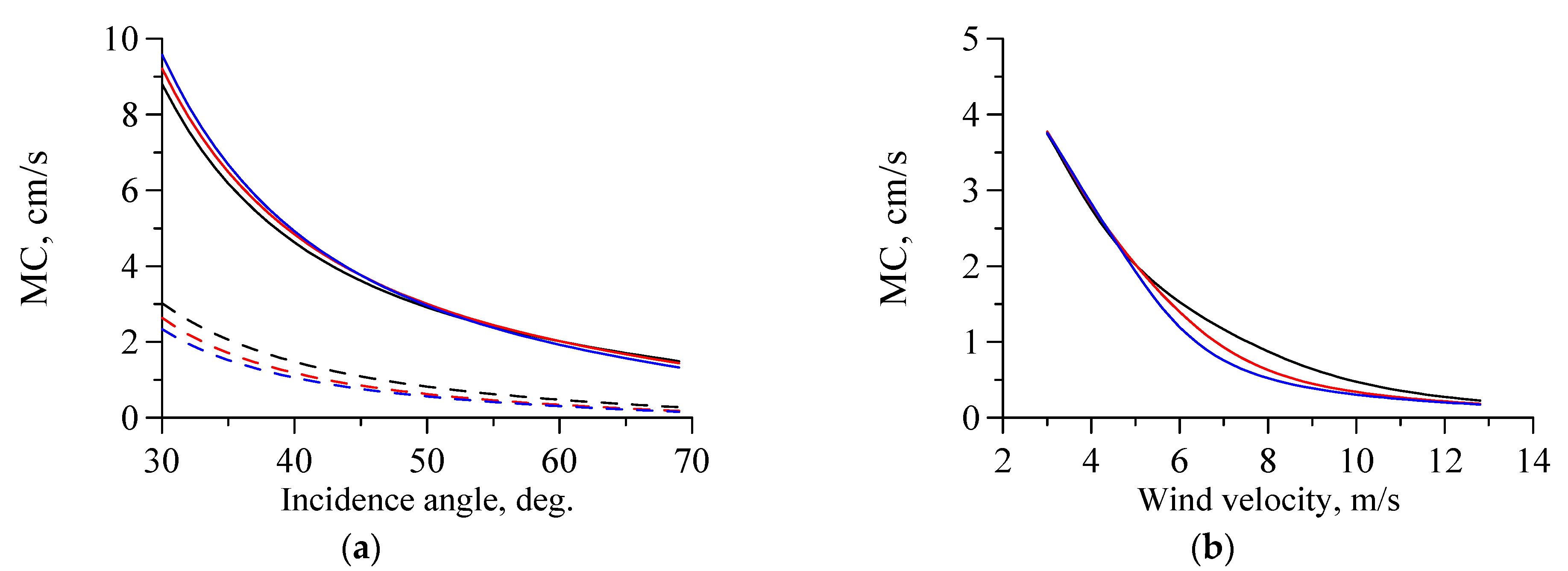
At low wind speeds, the illuminated area becomes comparable to the length of the modulating wave, which can be interpreted as an increase in the averaging time . We will estimate the effective time as , where is a size of the illuminated area in the observation direction or a length of one strobe on the surface. Figure 1a shows the dependence of the MC recalculated into the horizontal velocity on an incidence angle of radiation for appropriate wind speeds of 5 and 10 m/s. It can be seen that the MC value for a wind speed of 5 m/s exceeds the corresponding value for 10 m/s. The latter is because a period of the long waves becomes shorter as the wind decreases, and the illuminated area becomes comparable in size to the long wavelength. Figure 1b shows the dependence of the MC on wind speed for an incidence angle of 60 degrees. It can be seen that the MC in our case increases with decreasing wind speed and actually reaches its maximum value when the size of the illuminated area becomes comparable to the wavelength. At high wind speeds, when the size of the illuminated area becomes small compared to the long wavelength, the MC becomes small.
Since the sampling rate of the radar data is comparable to the frequency of the long wind wave, we can assume that the row radar data values are independent. The confidence interval for the scatterers velocities can be estimated as , where is a variance of the orbital velocity in the long wave, is a variance of the wave height determined mainly by the long waves, and is the number of the independent samples. Such estimation gives us the confidence interval of about 5 cm/s for an analysis time of about 10 min for a wind speed of 8–10 m/s.
4. Results
Two groups of case studies are presented below. In the first case study, a dependence of scatterer’s velocities at incidence angles of about 60 degrees were investigated with a falling wind. In the second case study, the scatterer’s velocities at different incidence angles with approximately constant wind were investigated. In addition, a large data base was accumulated for many series of our experiments on the relationship between scatterer’s velocities and wind speed for incidence angles of 60 degrees for different (uncontrolled) subsurface current velocities.
4.1. Scatterer’ Velocities with a Falling Wind
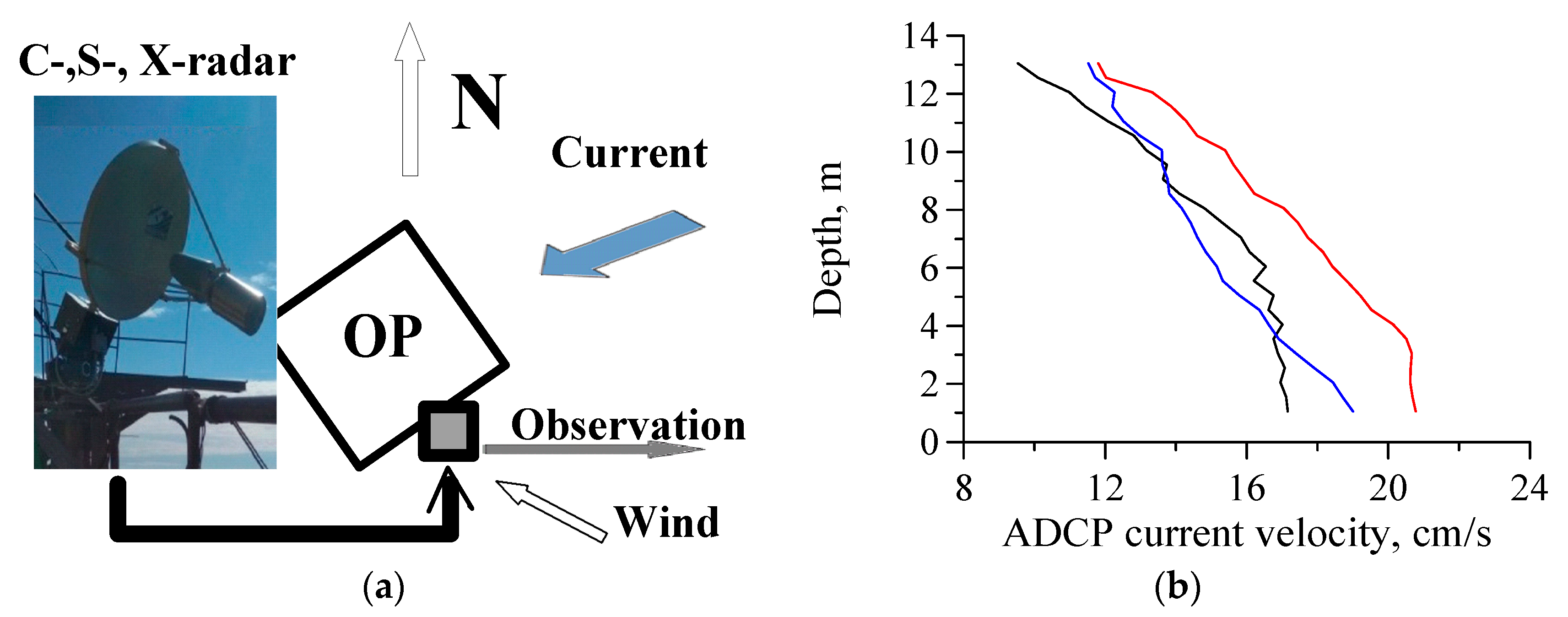
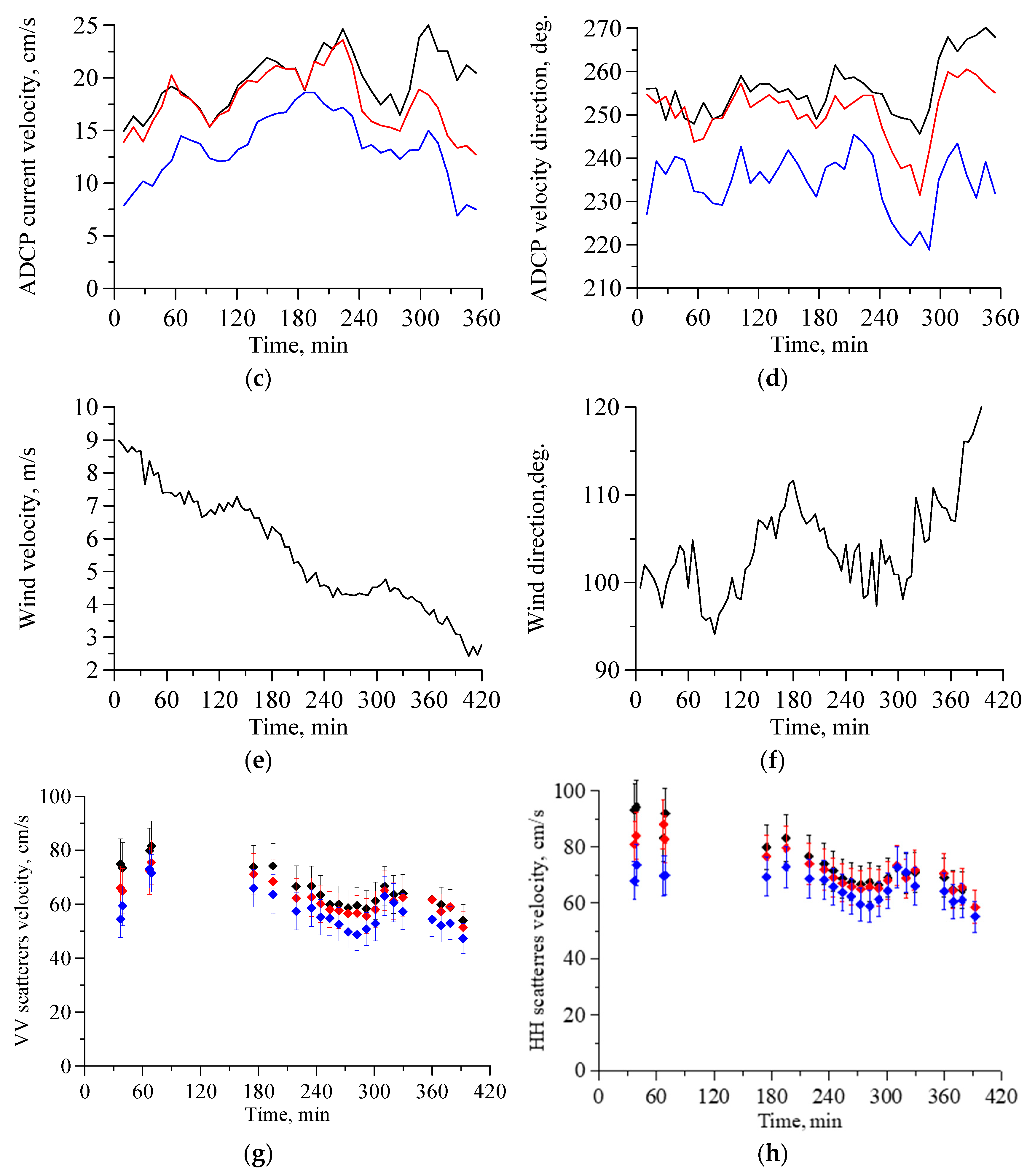
Figure 2 shows the scheme of our first case study (Figure 2a), the current velocity profiles measured by the ADCP (Figure 2b), time series of ADCP current (Figure 2c,d), wind (Figure 2e,f), and the horizontal projections of the scattering velocities at VV (Figure 2g) and HH (Figure 2h) polarizations.
One can see in Figure 2e,f that the wind speed decreases throughout the case study and the wind direction changes slightly (95 to 115 degrees), remaining close to the radar direction (90 degrees). Figure 2c,d show that in the first half of the case study, the ADCP current velocity at a depth of 1–4 m (the current did not change in depth) rises from 15 to 25 m/s, and the current direction remains nearly constant, about 20 degrees to the radar direction. In the second half of the case study, the current speed at a depth of 1 m varies between 25 and 15 m/s, and the current at a depth of 4 m has a lag behind the current at a depth of 1 m. The same effect is demonstrated in Figure 2b. At the beginning of the experiment, the velocity in the upper layer of about 1–5 m is practically unchanged, apparently due to sustained wind drift (wind speed was 8–10 m/s during the previous day), and at greater depths, it decreases slowly. At the end of the experiment, when the wind had already been decreasing for several hours, the current decreased at lower depths.
Figure 2g,h show that the scatterer’s velocity at HH polarization is greater than that at VV polarization. The scatterer’s velocities are greater for longer electromagnetic wave.
4.2. Scatterer’s Velocities with a Constant Wind
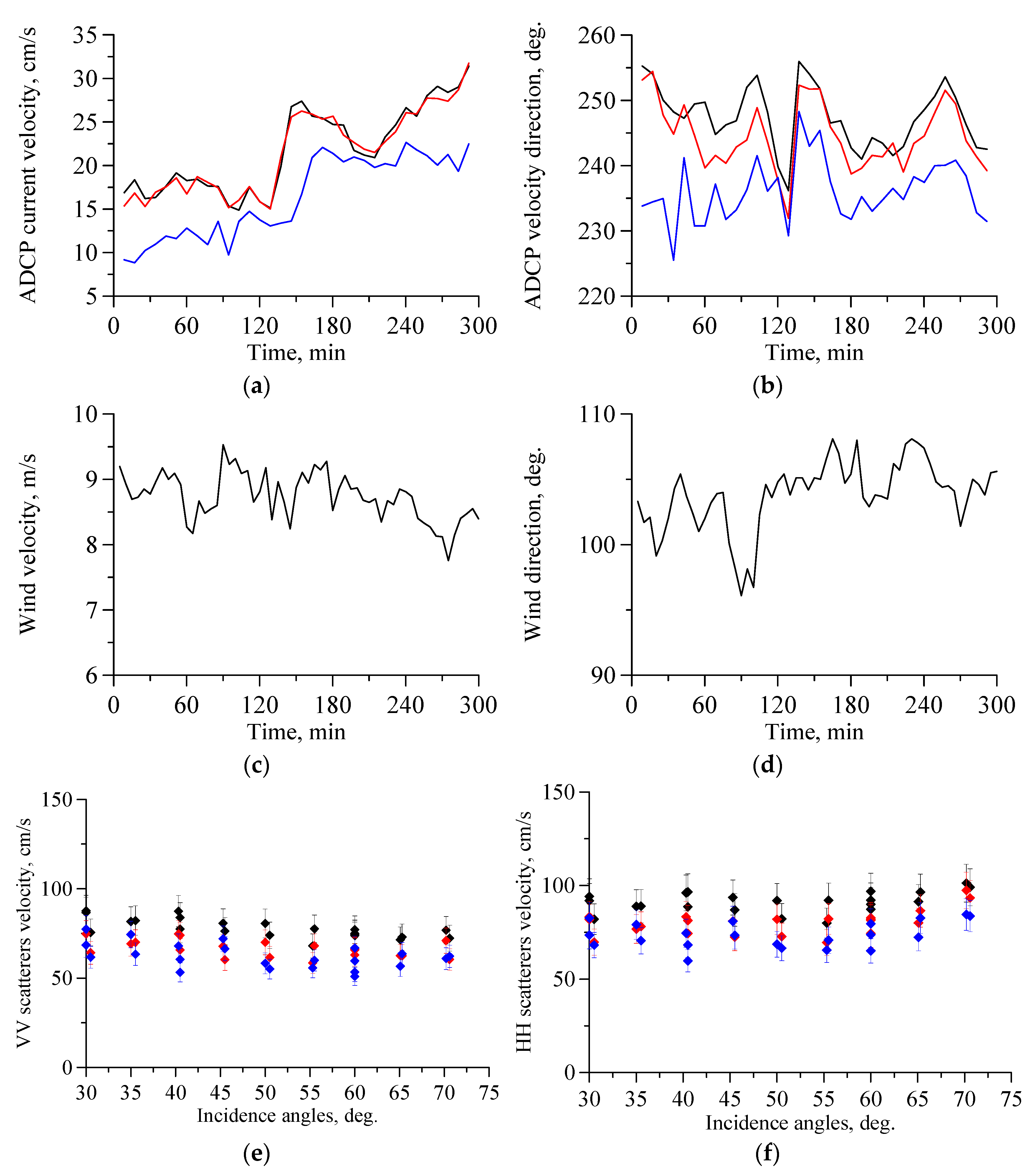
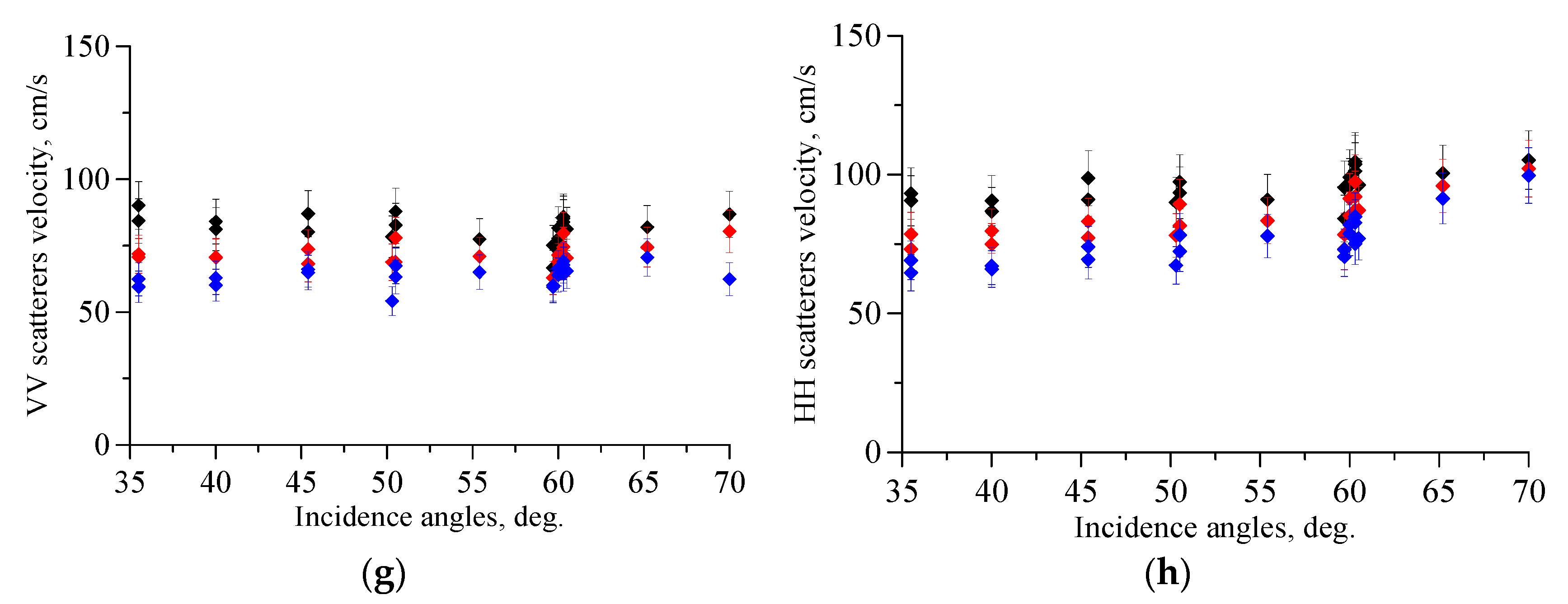
In the case study, measurements of the scatterer’s velocities were carried out at different incidence angles (30–70 degrees). Figure 3 shows time series of current velocities and directions (Figure 3a,b) (at depth of 1 m (black curve), 4 m (red curve), and 10 m (blue curve)), of wind (Figure 3c,d), and of the horizontal projections of the scatterers velocities at VV (Figure 3e) and HH (Figure 3f) polarizations on an incidence angle.
Figure 3c,d show that the wind speed (about 9 m/s) changes weakly during the experiment, and the angle between the direction of observation and the wind changes from 30 degrees to 20 degrees. The current in the upper layer (1–4 m) did not change in depth and direction. At greater depths, the speed decreased, and the current had a constant lag in direction. The current velocity in the upper layer in the first half of the experiment is less (approximately by 10 cm/s) than in the second half of the experiment; the direction of the current changes slightly, amounting to approximately 20–30 degrees to the observation direction.
As in experiment 4.1, the radar scatterer’s velocities increase with the radar wavelengths; the velocity of HH scatterers is greater than that of VV scatterers. The horizontal projection of the scatterer velocities weakly depends on the incidence angle of radiation. A small change in the sea current velocity at the beginning and end of the experiment is poorly visible, possibly due to a measurement error. It can be seen that the difference in the scatterer’s velocities at VV and HH polarizations increases with an incidence angle, which is due to the fact that at large incidence angles, the main scattering mechanism at VV polarization is the Bragg mechanism, and at HH polarization—non-Bragg mechanism (backscattering due long waves). At smaller incidence angles, the non-Bragg component significantly contributes to backscattering at both VV and HH polarizations.
Another case study on measurement of the scatterer’s velocity at two polarizations at different incidence angles is described and investigated in detail in [29]; the experiment was performed in weak winds, in the absence of strong wave breaking. Here, the same conclusions were drawn as for experiment 4.2.
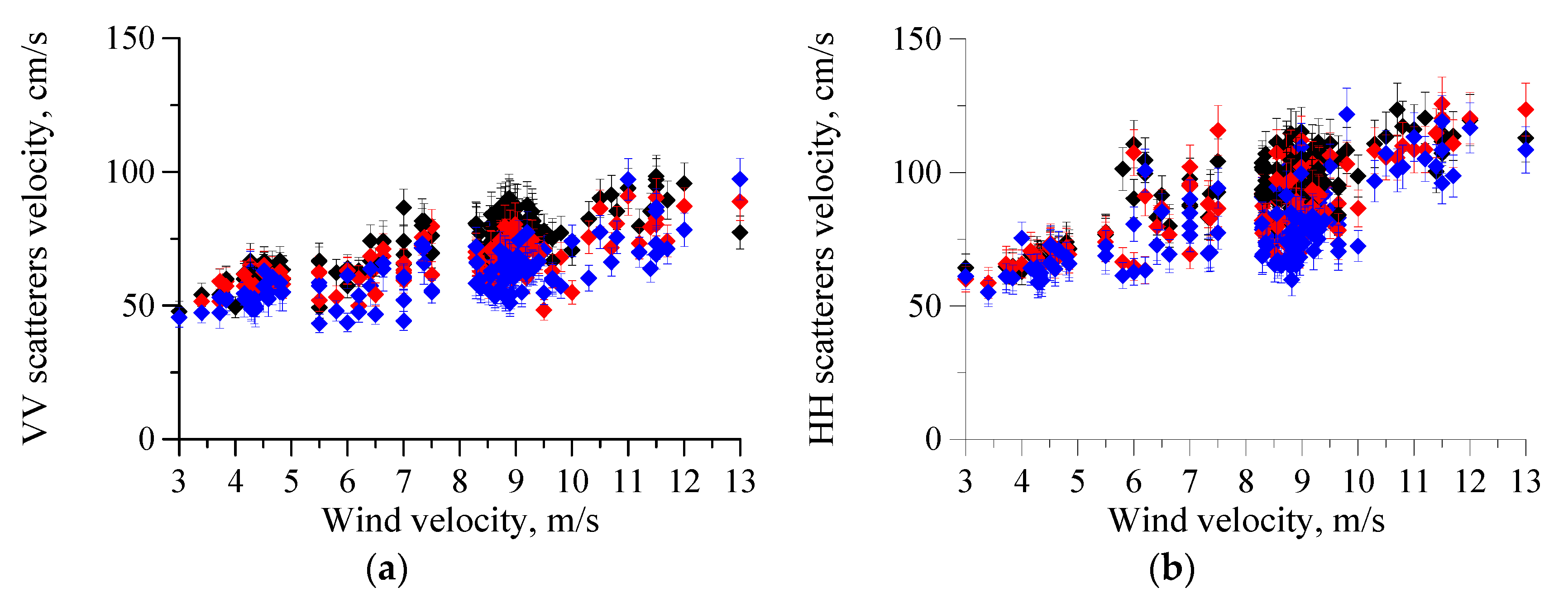
Scatter plots of the scatterer’s velocities at VV and HH polarizations and the wind velocities are presented in Figure 4. The experiments were carried out approximately against the wind and current (30 degrees from the direction of observation) at incidence angles of about 60 degrees. The data correspond to different series of experiments.
In Figure 4, it can be seen that the scatterer’s velocity both at VV, and HH polarizations increases with wind speed. A sharp increase in the HH scatterers’ speed is observed at wind speeds of 6–7 m/s, the latter is explained by the appearance of strong wave breaking associated with surface long fast waves which significantly contribute to scattering at HH polarization. The large scatter of the velocities, in our opinion, is due to different sea current velocities.
5. Discussion
5.1. Relation between Changes in ADCP Current Velocity and Subsurface Current Velocity Retrieved from the Polarization Difference
Let us discuss whether it is possible to detect any change in sea current velocity when analyzing the subsurface (SS) current velocity reconstructed from the polarization difference (i.e., in our model from the velocities of Bragg scatterers). Note that the ADCP measures the sea current velocity in depths of 1–15 m, while the depth at which the current significantly affects the Bragg wave propagation is comparable to the wavelength (i.e., is on the order of tens of cm). Thus, the ADCP does not measure the current, which we define as the subsurface one. Considering that the subsurface current is a vector sum of the sea current velocity and the wind drift velocity, let us see how the change in sea current reflects in the subsurface velocity.
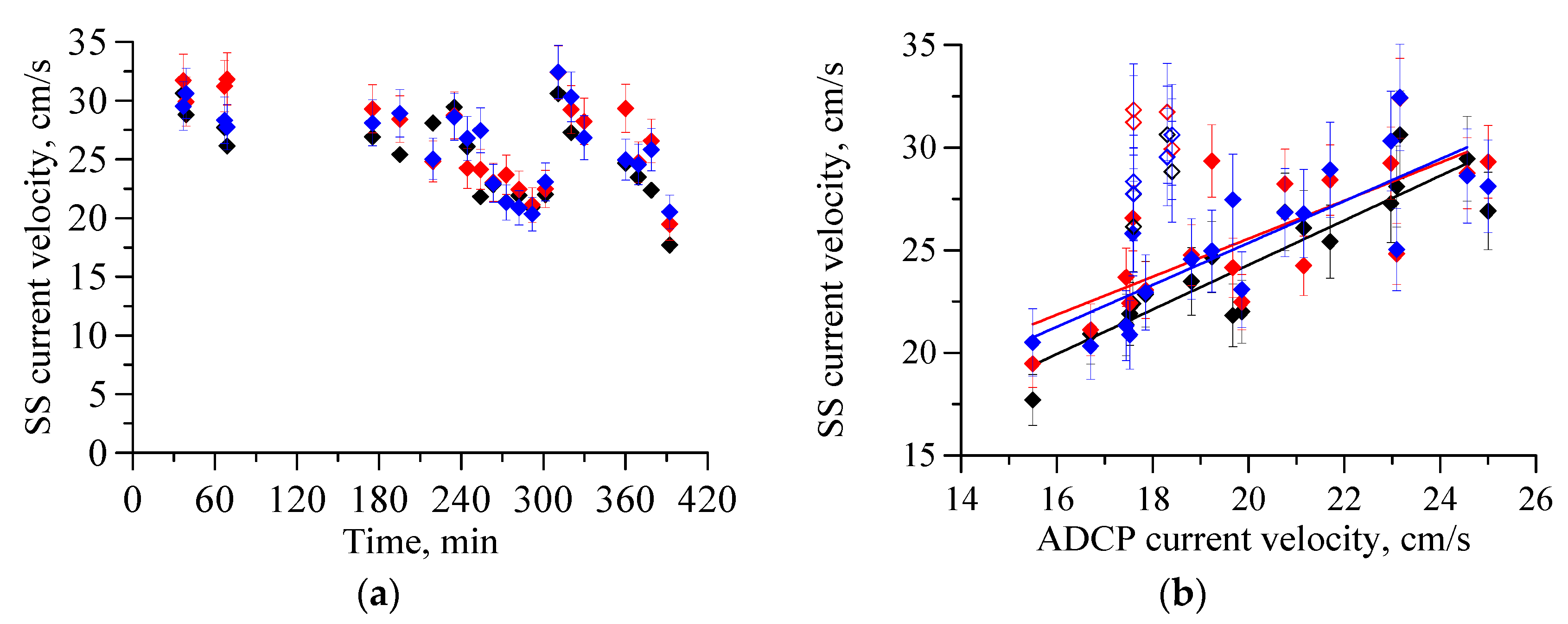
Remember that the polarization difference (PD) is determined only by the Bragg scattering mechanism, i.e., the Bragg waves with wavenumber . Let us assume that the wind waves are mostly free, i.e., propagate with velocities , g is the acceleration of gravity, is the surface tension at the air–water interface, and is the water density. The MC for the PD was estimated as shown in Section 3 and removed from the obtained PD value. Figure 5a shows time series of the SS current velocities (case study in 4.1). Figure 5b shows SS current velocities for different values of the sea current velocity at a depth of 1 m.
As illustrated in Figure 5a, the SS current velocities obtained from radar data are almost identical for three radar bands within the confidence interval. This is because the sea current varies slightly on scales of ten centimeters from the surface where the sea current affects the propagation of the Bragg waves. Figure 5b shows a scatter plot of the SS current velocities and sea velocities at a depth of 1 m. Solid symbols in Figure 5 correspond to wind speeds of 7–3 m/s, and open symbols to 8–9 m/s. The straight lines in Figure 5b are the line dependences of the SS velocity on the ADCP velocity for wind speeds of 3–7 m/s; the coefficient is 1.2, 0.95, and 1.1 for S-, C-, and X-band, respectively. The closeness of the coefficient to unity indicates a strong correlation between the SS current obtained from the radar data and the sea current.
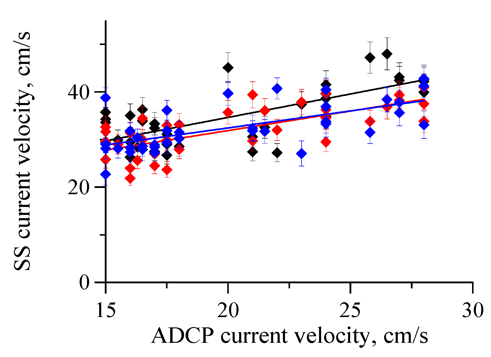
A scatter plot of the SS current velocity and sea current for case study 4.2 is presented in Figure 6. The coefficient is 0.9, 0.8, and 0.7 for S-, C-, and X-band, respectively. Thus, Figure 5b and Figure 6 demonstrate that the variations in the sea current velocity in the upper layer can be detected from the change in the Bragg scatterer’s velocity (the velocity of the PD difference scatterers) at a constant (slightly varying) wind speed.
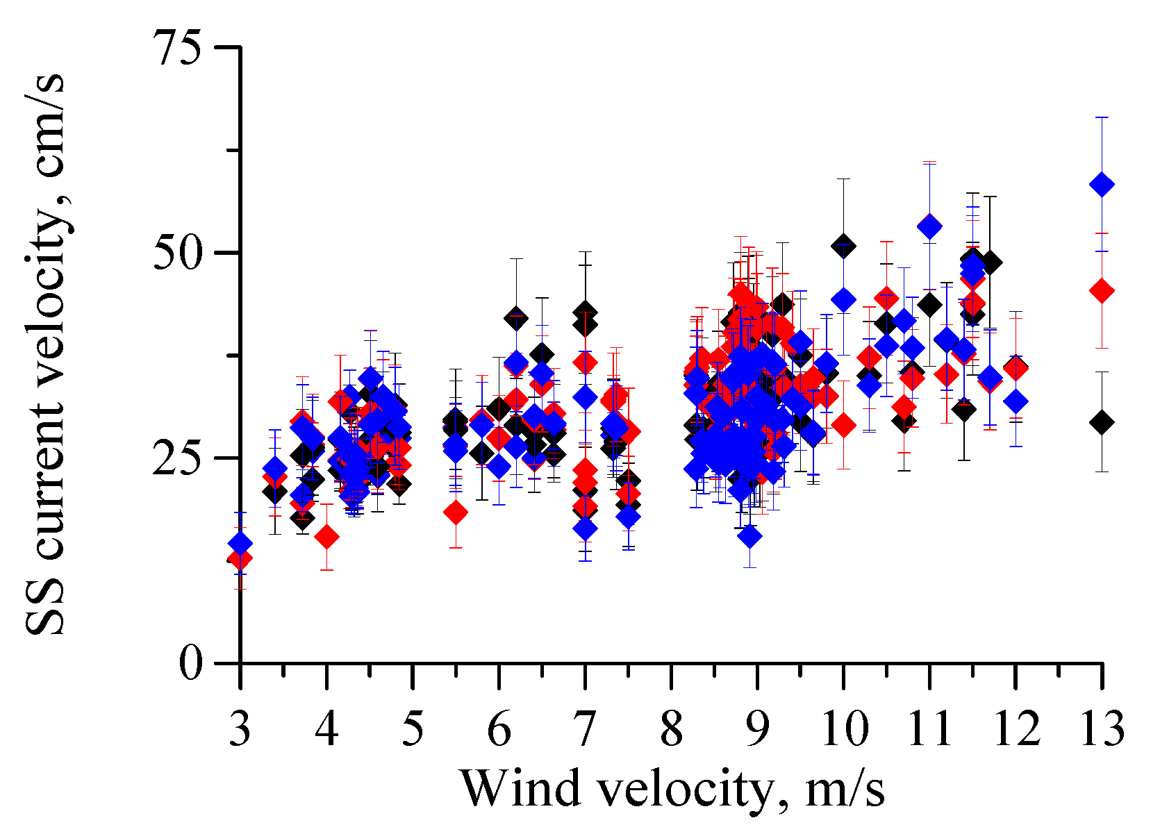
Figure 7 illustrates the relationship between the SS current velocity and the wind speeds, in which the incidence angles were about of 60 degrees (data from Figure 4). Here, one can see the strong dependence of the subsurface current velocity on wind speed.
Thus, it can be concluded that the SS current velocity retrieved from microwave radar data strongly depends on the wind speed. However, the SS current can be used to estimate the change of current velocity in the upper layer at a constant wind speed.
5.2. A Problem of Estimating the Marine Current Speed from the Subsurface Current Velocity
However, the assessment of absolute values of the marine current velocity from the value of the SS current velocity still remains problematic. In a number of works (see, e.g., [2,20] and references therein), it is proposed to consider the current on the sea surface as a vector sum of a “marine” current (independent of wind) velocity and wind component as fixed percentage of wind speed. The problem is that nobody knows at what depth the current becomes independent of the wind and we can consider it a marine current. If the current changes with depth, we must take the different values of wave components for different depths (where we consider the current to be marine) to obtain the measured velocity value in the upper layer (i.e., SS current velocity). Let us introduce wind deposit (WD), which we define as a difference between the SS current velocity () and ADCP velocity (i.e., wind component), divided by the wind speed.
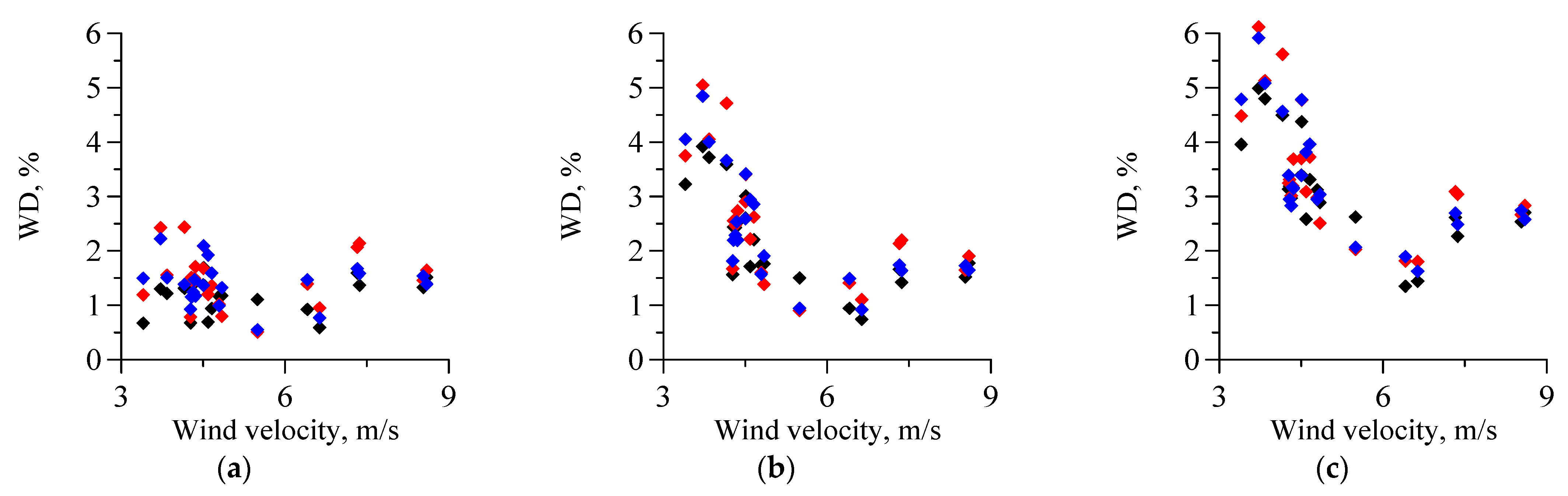
Note that if is a velocity of “marine” current, then is equal to wind drift velocity in the upper layer. Figure 8 shows the WD for the case study 4.1. Here, the ADCP velocity was measured at depths of 1 m, 4 m, and 10 m. We are interested in depths down to 10 m, as we believe that at greater depths, the seabed affects the current.
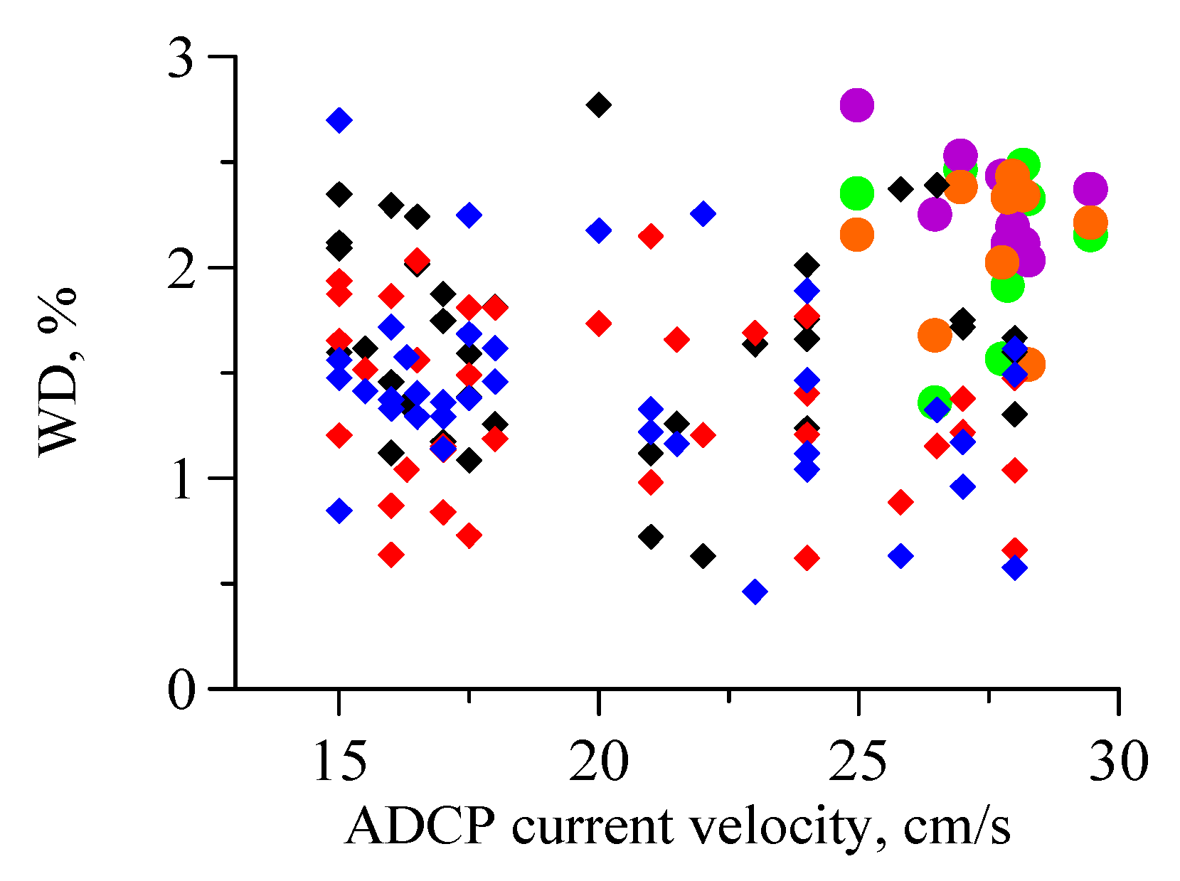
Since the ADCP current speed decreases with depth, one can expect that the WD increases with the depth at which the ADCP current is measured, as can be seen in Figure 8. The current at a depth of 1 m (see, Figure 2b) is not the “marine” one for both moderate and low wind. Here, WD is 1–2%, i.e., the wind component is linearly dependent on the wind velocity. At a depth of 4 m, the WD is strongly dependent on wind speed; it increases significantly at low speeds, remaining almost constant at higher speeds. The effect can be due to the fact that in weak wind, the current at a depth of 1 m is closer to the “marine” current, while for moderate wind, the sea current is not the “marine” one (here, WD is constant). However, it can be also due to the fact that in a falling wind, the SS current corresponds to the higher wind values than those obtained at the same time as the current was measured. At moderate wind speeds (at the beginning of the case study), the wind current corresponded to the simultaneously measured wind speed (remember that the winds have been consistently moderate all day). So, to estimate correctly the current speed in the upper layer from the SS current velocity, some additional information about the wind (prehistory) is needed. It can be seen that the WD for moderate wind speeds is of the order of or less than 2%, whatever depth of the “marine” current we choose. Figure 9 shows the WD for case study 4.2.; some data from [29] for a wind speed of 5–6 m/s are also presented here. In both cases, before and during the experiments, the wind was steady. It can be seen that the WD values vary within the same limits 1–3%. However, to determine the value of current velocity at other depths, it is necessary to know the features of wave drift and sea current formation, which is not considered in the paper. So, the problem of choosing the depth at which the current velocity can be considered as the “marine” one remains unresolved. From our study, one can conclude that the depth is determined, among other things, by the wind speed and its stability (fetch, profile). It should be recognized that the study of the formation of sea currents is beyond the scope of this paper.
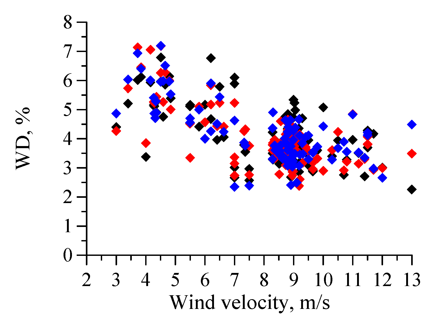
Let us see what WD will be if we do not take into account sea current at all. Figure 10 shows the WD values for the data from Figure 4. It can be seen that the WD decreases with wind speed. The latter is due to the fact that the term in (6) decreases. The data in Figure 10 allow us to perform a very rough estimate of the SS current speed at moderate current speeds only from the wind speed in the coastal zone of the Black Sea. Note that these results have, of course, “regional” character.
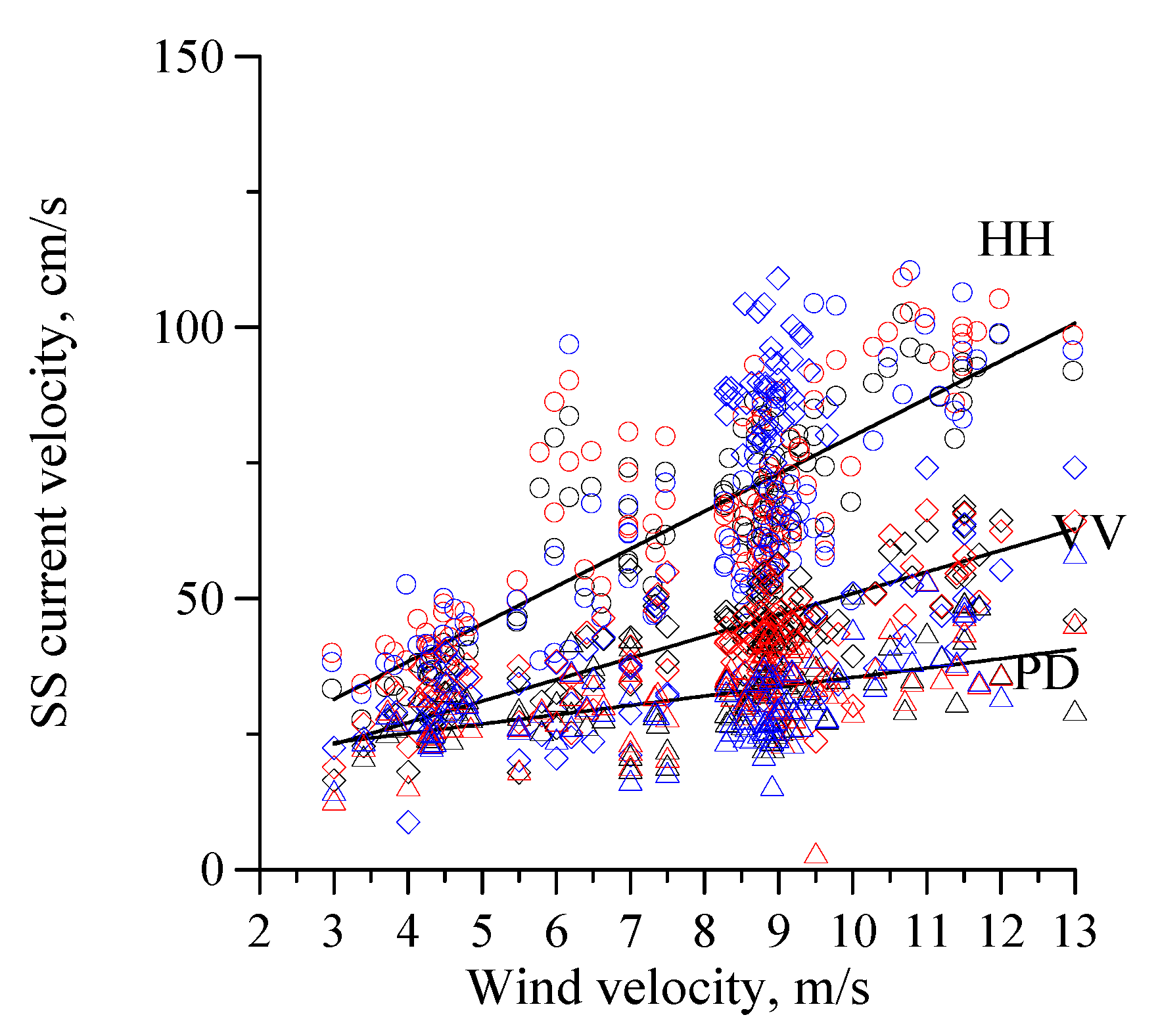
Figure 11 demonstrates the SS current velocity, retrieved from data at VV and HH polarizations and from the polarization difference at moderate incidence angles (60–70 degrees), as functions on a wind speed. In all cases, we assumed that the radar scatterers were the free Bragg waves. The straight lines are the average velocities in the S-band. Open symbols are our experimental data. It can be seen that the difference in the subsurface current velocities determined from the VV polarization and from the PD does not exceed 20 cm/s, while the difference in the SS current velocities obtained from the HH polarization data and from PD is up to 50–60 cm/s. The latter is explained by the fact that scatterers at HH and VV polarizations are wind waves with longer wavelength than the Bragg one, propagating with higher speeds [12,13]. So, to determine the SS velocity from data at VV and HH polarizations, it is necessary to subtract other velocities of scatterers. It is worth noting that non-Bragg scattering is poorly understood by now and more research is needed.
Note that since the SS current velocities obtained from the VV/HH/PD data are different, and in some cases significantly different, estimates of the values of current velocities from data at the VV/HH polarizations are problematic. However, the variations of current velocities can be detected using data of a radar operating at one (VV or HH) polarization.
6. Conclusions
Simultaneous measurements of microwave scatterers’ velocities using a dual-polarized Doppler radar operating in the S-, C-, and X-bands, as well as measurements of sea current and wind speed, were carried out. The velocity of the scatterers was obtained as a centroid of the Doppler spectrum. Measurements were made at incidence angles of 30–70 degrees and wind speed of 3–9 m/s in approximately upwind and downwind directions in the coastal zone of the Black Sea. The subsurface current velocity, determined from a polarization difference (the Bragg scatterer’s velocity), is analyzed with wind and sea current variations.
It is shown that variations in the upper sea current velocity can be detected from changes in the subsurface current velocity retrieved from radar data at constant wind speed.
The subsurface current velocity (current in a layer of a few dm) obtained from the polarization difference is equal to a vector sum of the current velocity measured by ADCP at a depth of 1 m and the wind component equal to 1–3% of the wind speed. We found that the ratio of the wind component at a certain depth to the wind speed increases with depth and decreases with wind speed. This is due to the fact that the current velocity below the surface decreases with depth, and it decreases faster in weak winds than in moderate winds.
The results obtained in the study can be used to model marine currents in the upper layer (e.g., to predict the spread of contaminants at the sea surface) and to estimate marine current variations.
Author Contributions
Conceptualization, I.K. and S.E.; methodology, I.K. and I.S.; investigation, L.P.; data curation, I.K. and A.K.; writing, I.S. and S.E.. All authors have read and agreed to the published version of the manuscript.
Funding
This work was supported by the Russian Science Foundation, Project No. 18-77-10066. Conceptualization and writing by S. Ermakov was supported by the state assignment FFUF-2021-0006.
Data Availability Statement
All the related data are available from the corresponding author upon reasonable request.
Acknowledgments
The authors are grateful to A.A. Molkov for his help in the measurements.
Conflicts of Interest
The authors declare no conflict of interest.
References
- Klemas, V. Remote sensing of coastal and ocean currents: An overview. J. Coast. Res. 2012, 28, 576–586. [Google Scholar] [CrossRef]
- Elyouncha, A.; Eriksson, L.E.B.; Romeiser, R.; Ulander, L.M.H. Empirical Relationship between the Doppler Centroid Derived from X-Band Spaceborne InSAR Data and Wind Vectors. IEEE Trans. Geosci. Remote Sens. 2022, 60, 4201120. [Google Scholar] [CrossRef]
- Martin, A.C.H.; Gommenginger, C.P.; Jacob, B.; Staneva, J. First multi-year assessment of Sentinel-1 radial velocity products using HF radar currents in a coastal environment. Remote Sens. Environ. 2022, 268, 112758. [Google Scholar] [CrossRef]
- Wang, L.; Shi, B.; Zhou, Y.; Sheng, H.; Gao, Y.; Fan, L.; Yang, Z. Radial velocity of ocean surface current estimated from SAR Doppler frequency measurements—A case study of Kuroshio in the East China Sea. Acta Oceanol. Sin. 2021, 40, 135–147. [Google Scholar] [CrossRef]
- Moiseev, A.; Johnsen, H.; Johannessen, J.A. Retrieving Ocean Surface Currents from the Sentinel-1 Doppler Shift Observations: A Case Study of the Norwegian Coastal Current. In Proceedings of the IEEE International Geoscience and Remote Sensing Symposium, Waikoloa, HI, USA, 26 September–2 October 2020; pp. 5670–5673. [Google Scholar] [CrossRef]
- Moiseev, A.; Johnsen, H.; Hansen, M.W.; Johannessen, J.A. Evaluation of radial ocean surface currents derived from Sentinel-1 IW Doppler shift using coastal radar and Lagrangian surface drifter observations. J. Geophys. Res. Oceans 2020, 125, e2019JC015743. [Google Scholar] [CrossRef]
- Mouche, A.A.; Collard, F.; Chapron, B.; Dagestad, K.-F.; Guitton, G.; Johannessen, J.A.; Kerbaol, V.; Hansen, M.W. On the Use of Doppler Shift for Sea Surface Wind Retrieval from SAR. IEEE Trans. Geosci. Remote Sens. 2012, 50, 2901–2909. [Google Scholar] [CrossRef]
- Chapron, B.; Collard, F.; Ardhuin, F. Direct measurements of ocean surface velocity from space: Interpretation and validation. J. Geophys. Res. 2005, 110, C07008. [Google Scholar] [CrossRef]
- Bass, F.G.; Fuks, M. Wave Scattering from Statistically Rough Surfaces; Pergamon: Oxford, UK, 1979; p. 540. ISBN 9781483187754. [Google Scholar]
- Valenzuela, G.R. Theories for the interaction of electromagnetic and oceanic waves—A review. Bound. Layer Meteorol. 1978, 13, 61–85. [Google Scholar] [CrossRef]
- Voronovich, A.G.; Zavorotny, V.U. A numerical model of radar scattering from steep and breaking waves. In Proceedings of the IEEE International Geoscience and Remote Sensing Symposium, Denver, CO, USA, 31 July–4 August 2006; pp. 469–472. [Google Scholar] [CrossRef]
- Fois, F.; Hoogeboom, P.; Le Chevalier, F.; Stoffelen, A. An analytical model for the description of the full polarimetric sea surface Doppler signature. J. Geophys. Res. Oceans 2015, 120, 988–1015. [Google Scholar] [CrossRef] [Green Version]
- Kudryavtsev, V.; Hauser, D.; Caudal, G.; Chapron, B. A semi-empirical model of the normalized radar cross section of the sea surface. 1. Background model. J. Geophys. Res. 2003, 108, 8054. [Google Scholar] [CrossRef] [Green Version]
- Ermakov, S.A.; Sergievskaya, I.A.; da Silva, J.C.B.; Kapustin, I.A.; Shomina, O.V.; Kupaev, A.V.; Molkov, A.A. Remote Sensing of Organic Films on the Water Surface Using Dual Co-Polarized Ship-Based X-/C-/S-Band Radar and TerraSAR-X. Remote Sens. 2018, 10, 1097. [Google Scholar] [CrossRef] [Green Version]
- Sergievskaya, I.A.; Ermakov, S.A.; Ermoshkin, A.V.; Kapustin, I.A.; Molkov, A.A.; Danilicheva, O.A.; Shomina, O.V. Modulation of Dual-Polarized X-Band Radar Backscatter due to Long Wind Waves. Remote Sens. 2019, 11, 423. [Google Scholar] [CrossRef] [Green Version]
- Sergievskaya, I.A.; Ermakov, S.A.; Ermoshkin, A.V.; Kapustin, I.A.; Shomina, O.V.; Kupaev, A.V. The Role of Micro Breaking of Small-Scale Wind Waves in Radar Backscattering from Sea Surface. Remote Sens. 2020, 12, 4159. [Google Scholar] [CrossRef]
- Martin, A.C.H.; Gommenginger, C.; Marquez, J.; Doody, S.; Navarro, V.; Buck, C. Wind-wave-induced velocity in ATI SAR ocean surface currents: First experimental evidence from an airborne campaign. J. Geophys. Res. Oceans 2016, 121, 1640–1653. [Google Scholar] [CrossRef] [Green Version]
- Nouguier, F.; Chapron, B.; Collard, F.; Mouche, A.A.; Rascle, N.; Ardhuin, F.; Wu, X. Sea Surface Kinematics from Near-Nadir Radar Measurement. IEEE Trans. Geosci. Remote Sens. 2018, 56, 6169–6179. [Google Scholar] [CrossRef]
- Ermakov, S.A.; Sergievskaya, I.A.; Zuikova, E.M.; Shchegol’kov, Y.B. Modulation of Radar Backscatter by Long Waves on the Sea Surface Covered with a Surfactant Film. Izv. Atmos. Ocean. Phys. 2004, 4, 91–98. [Google Scholar]
- Kapustin, I.A.; Shomina, O.V.; Ermoshkin, A.V.; Bogatov, N.A.; Kupaev, A.V.; Molkov, A.A.; Ermakov, S.A. On Capabilities of Tracking Marine Surface Currents Using Artificial Film Slicks. Remote Sens. 2019, 11, 840. [Google Scholar] [CrossRef] [Green Version]
- Wu, J. Wind-induced drift currents. J. Fluid Mech. 1975, 68, 49–70. [Google Scholar] [CrossRef]
- Wu, J. Sea-surface drift currents induced by wind and waves. J. Geophys. Res. 1983, 13, 1441–1451. [Google Scholar] [CrossRef]
- Van der Mheen, M.; Pattiaratchi, C.; Cosoli, S.; Wandres, M. Depth-Dependent Correction for Wind-Driven Drift Current in Particle Tracking Applications. Front. Mar. Sci. 2020, 7, 305. [Google Scholar] [CrossRef]
- Leibovich, S. On the evolution of the system of wind drift currents and Langmuir circulations in the ocean. Part 1. Theory and averaged current. J. Fluid Mech. 1977, 79, 715–743. [Google Scholar] [CrossRef]
- Phillips, O.M. Radar returns from the sea surface—Bragg scattering and breaking waves. J. Phys. Oceanogr. 1988, 18, 1065–1074. [Google Scholar] [CrossRef]
- Troitskaya, Y.I. Modulation of the growth rate of short, surface capillary-gravity wind waves by a long wave. J. Fluid Mech. 1994, 273, 169–187. [Google Scholar] [CrossRef]
- Hara, T.; Plant, W.J. Hydrodynamic modulation of short wind-wave spectra by long waves and its measurement using microwave backscatter. J. Geophys. Res. 1994, 99, 9767–9783. [Google Scholar] [CrossRef]
- Plant, W.J. The Modulation Transfer Function: Concept and Applications. In Radar Scattering from Modulated Wind Waves, 1st ed.; Komen, G.J., Oost, W.A., Eds.; Springer: Dordrecht, The Netherlands, 1989; pp. 155–172. [Google Scholar] [CrossRef]
- Sergievskaya, I.A.; Ermakov, S.A.; Plotnikov, L.M.; Kapustin, I.A.; Ermoshkin, A.V. On the estimation of surface current velocities from microwave sea surface measurements at moderate incidence angles. Sovr. Probl. DZZ Kosm. 2022, 19, 212–222. [Google Scholar] [CrossRef]
Figure 1.
(a) MC vs. incidence angle (PD). Black curves are S-band, red—C-band, blue—X-band, dashed curves are 10 m/s, solid curves are 5 m/s. (b) MC vs. wind speed. Black curves are S-band, red are C-band, and blue are X-band. Incidence angle is 60 degrees.
Figure 1.
(a) MC vs. incidence angle (PD). Black curves are S-band, red—C-band, blue—X-band, dashed curves are 10 m/s, solid curves are 5 m/s. (b) MC vs. wind speed. Black curves are S-band, red are C-band, and blue are X-band. Incidence angle is 60 degrees.

Figure 2.
Case study 4.1. (a) Schematic representation. (b) The ADCP current velocity profiles in the beginning (black), middle (red), and end (blue) of the case study. (c) The ADCP current velocity and (d) direction at depths of 1 m (black curve), 4 m (red curve), and 10 m (blue curve). (e) The wind velocity and (f) direction. (g) The scatterer’ velocities at VV and (h) HH polarizations. Black symbols correspond to S-band, red—C-band, blue—X-band.


Figure 3.
Case study 4.2. (a) The velocity and (b) direction of ADCP current at depths of 1 m (black curve), 4 m (red curve), and 10 m (blue curve). (c) The wind speed and (d) direction. The scatterer’s velocity for the radar return at VV (e) 0–150 min, (g) 150–300 min and HH (f) 0–150 min, (h) 150–300 min polarizations. Black dots are S-band, red—C-band, blue—X-band.


Figure 4.
(a) The scatterer velocities at VV and (b) HH polarizations vs. the wind velocity. Black symbols—S-band, red—C-band, blue—X-band.
Figure 4.
(a) The scatterer velocities at VV and (b) HH polarizations vs. the wind velocity. Black symbols—S-band, red—C-band, blue—X-band.

Figure 5.
(a) Time series of the subsurface current velocities. (b) Subsurface current velocity vs. ADCP current velocity at a depth of 1 m. Case study 4.1. Black dots—S-band, red—C-band, blue—X-band. Solid symbols-wind speed 7–3 m/s; open symbols-8–9 m/s.
Figure 5.
(a) Time series of the subsurface current velocities. (b) Subsurface current velocity vs. ADCP current velocity at a depth of 1 m. Case study 4.1. Black dots—S-band, red—C-band, blue—X-band. Solid symbols-wind speed 7–3 m/s; open symbols-8–9 m/s.

Figure 6.
Subsurface current velocity vs. ADCP current velocity at a depth of 1 m. Case study 4.2. Black symbols—S-band, red—C-band, blue—X-band.
Figure 6.
Subsurface current velocity vs. ADCP current velocity at a depth of 1 m. Case study 4.2. Black symbols—S-band, red—C-band, blue—X-band.

Figure 7.
Subsurface current velocities vs. wind speeds (from Figure 4). Black symbols—S-band, red—C-band, blue—X-band.
Figure 7.
Subsurface current velocities vs. wind speeds (from Figure 4). Black symbols—S-band, red—C-band, blue—X-band.

Figure 8.
Case study 4.1. WD vs. wind speed (minus the current speed at depths of (a) 1 m, (b) 4 m, and (c) 10 m). Black symbols—S-band, red—C-band, blue—X-band.
Figure 8.
Case study 4.1. WD vs. wind speed (minus the current speed at depths of (a) 1 m, (b) 4 m, and (c) 10 m). Black symbols—S-band, red—C-band, blue—X-band.

Figure 9.
WD in the case study 4.2. vs. ADCP current velocity (minus current velocity at a depth of 1 m). Black/green symbols—S-band, red/violet—C-band, blue/orange—X-band, diamonds—case study 4.2, circles—[29].
Figure 9.
WD in the case study 4.2. vs. ADCP current velocity (minus current velocity at a depth of 1 m). Black/green symbols—S-band, red/violet—C-band, blue/orange—X-band, diamonds—case study 4.2, circles—[29].

Figure 10.
Ratio of subsurface current velocity to wind velocity (data from Figure 4). Black symbols—S-band, red—C-band, blue—X-band.
Figure 10.
Ratio of subsurface current velocity to wind velocity (data from Figure 4). Black symbols—S-band, red—C-band, blue—X-band.

Figure 11.
The velocities of VV/HH/Bragg scatterers and subsurface current velocity determined from VV/HH/PD vs. wind velocity. Black symbols—S-band, red—C-band, blue—X-band, circles—HH, diamonds—VV, triangle—PD.
Figure 11.
The velocities of VV/HH/Bragg scatterers and subsurface current velocity determined from VV/HH/PD vs. wind velocity. Black symbols—S-band, red—C-band, blue—X-band, circles—HH, diamonds—VV, triangle—PD.

Disclaimer/Publisher’s Note: The statements, opinions and data contained in all publications are solely those of the individual author(s) and contributor(s) and not of MDPI and/or the editor(s). MDPI and/or the editor(s) disclaim responsibility for any injury to people or property resulting from any ideas, methods, instructions or products referred to in the content. |
© 2023 by the authors. Licensee MDPI, Basel, Switzerland. This article is an open access article distributed under the terms and conditions of the Creative Commons Attribution (CC BY) license (https://creativecommons.org/licenses/by/4.0/).
Share and Cite
MDPI and ACS Style
Sergievskaya, I.; Ermakov, S.; Plotnikov, L.; Kapustin, I.; Kupaev, A. On a Problem of Marine Current Velocity Estimation from Microwave Radar Data. Water 2023, 15, 1153. https://doi.org/10.3390/w15061153
AMA Style
Sergievskaya I, Ermakov S, Plotnikov L, Kapustin I, Kupaev A. On a Problem of Marine Current Velocity Estimation from Microwave Radar Data. Water. 2023; 15(6):1153. https://doi.org/10.3390/w15061153
Chicago/Turabian StyleSergievskaya, Irina, Stanislav Ermakov, Leonid Plotnikov, Ivan Kapustin, and Alexander Kupaev. 2023. "On a Problem of Marine Current Velocity Estimation from Microwave Radar Data" Water 15, no. 6: 1153. https://doi.org/10.3390/w15061153
Note that from the first issue of 2016, this journal uses article numbers instead of page numbers. See further details here.