Article

A Coupled Seepage–Deformation Model for Simulating the Effect of Fracture Seepage on Rock Slope Stability Using the Numerical Manifold Method

1
Beijing Research Center for Engineering Structures and New Materials, Beijing University of Civil Engineering and Architecture, Beijing 100044, China
2
School of Civil and Transportation Engineering, Beijing University of Civil Engineering and Architecture, Beijing 100044, China
3
Department of Civil, Environmental and Geomatic Engineering, University College London, London WC1E 6BT, UK
4
Department of Civil Engineering, The University of Edinburgh, Edinburgh EH8 9YL, UK
5
Department of Mechanical Engineering, The University of Western Australia, Perth, WA 6009, Australia
6
Department of Civil, Environmental and Mining Engineering, The University of Western Australia, Perth, WA 6009, Australia
*
Author to whom correspondence should be addressed.
These authors contributed equally to this work.
Water 2023, 15(6), 1163; https://doi.org/10.3390/w15061163
Submission received: 6 February 2023 / Revised: 5 March 2023 / Accepted: 14 March 2023 / Published: 17 March 2023
(This article belongs to the Special Issue Effects of Groundwater and Surface Water on the Natural Geo-Hazards)

Abstract

:
Modeling seepage problems in rock fractures is an interesting research approach to evaluating rock slope instability that is attracting increasing attention. In the present study, a coupled seepage–deformation model based on the numerical manifold method (NMM) is proposed, and the flow of groundwater in a fracture network coupled with the effects of seepage pressure and rock deformation are discussed. A global equilibrium equation of the system and a local factor of safety (FoS) of arbitrary rock fractures are derived based on the principle of minimum energy, and a series of verification examples are calculated. The simulation results show the robustness and effectiveness of the proposed numerical model. Finally, a rock slope collapse accident caused by seepage effects is simulated by the proposed method, and the failure process of the slope is reproduced. The simulation results show that excessive hydraulic pressure caused the vertical fractures to open and augmented the rock mass deformation, eventually leading to the failure of the slope. The proposed method possesses the potential to simulate larger-scale engineering problems.

1. Introduction

The stability of rock slopes is currently a hot topic in rock engineering and rock mechanics [1,2]. Normally, there are multiple discontinuities within a rock mass, such as joints and fractures, which often reduce the strength of the rock mass and cause failure of the rock slope. In addition, these discontinuities can serve as groundwater flow channels, forming fracture seepage networks [3]. Seepage pressure and the hydraulic head of the groundwater act on both surfaces of the fracture, which induces both hydrostatic pressure and seepage forces, leading to rock deformation, changes in fracture aperture and permeability, and even evolution of the fracture network (e.g., reducing the friction coefficient and strength of the fracture) [4]. On the other hand, changes in the state of fractures back influence the fluid flow, as shown in Figure 1: when the hydraulic pressure on the fracture interface is greater than the normal contact compression, the fractures will open or expand. Thus, it is critical to consider a hydro-mechanical coupling model using numerical simulations when seepage-deformation problems of rock fracture interaction are encountered. In addition, engineering practices show that the rise of groundwater levels and seepage in fractures are important causes of rock slope instability [5,6,7]. Therefore, it is essential to develop a coupled seepage–deformation model to study the influence of fracture seepage on rock slope stability.
The theoretical development in this field started with Biot [8], who proposed a theory of poro-elasticity for a porous medium saturated with an incompressible fluid to consider the coupled seepage–deformation mechanism. Rice and Cleary [9] extended the theory to account for a compressible fluid. However, Biot’s theory is based on a continuum theory, and no interactions between fractures are taken into consideration. Curran and Carvalho [10,11] further extended the theory to include the effect of deformation of one fracture on other fractures. Because of the complexity of fluid–solid interactions and subsequent stress-induced fracture evolution, developing analytical models to realistically account for such a complex process presents a challenge.
As an alternative to analytical models, numerical models of coupled hydro–mechanical processes were developed based on Biot’s theory for porous media to simulate the coupling effect of fracture seepage and rock deformation [12,13,14,15,16]. Normally, numerical models can be classified into two categories: continuum-based models and discontinuous models that include fractures or joints. In continuum models, e.g., finite element models (FEMs) and phase-field methods (PFMs), a rock mass with joints and fractures is modeled as a porous continuum whose properties take into account the information of joints/fractures. In such a model, porosity and permeability coefficients are applied to simulate the seepage–deformation coupling effect of fractured rock [12,13,14]. However, the model usually ignores local seepage features, as only a homogenized seepage deformation law is used.
As an alternative, the discontinuous model combines the flow of fluid along the fracture network and the effect of hydraulic pressure on the fracture interface [17]. Recently developed discrete numerical methods, such as the distinct element method (DEM) [18,19] and discontinuous deformation analysis (DDA) [3,20,21], treat the rock cut by joint fissures as a discontinuum in which each cut block is regarded as a computational element. The whole block system and fracture network are constructed by introducing contact springs between the blocks; seepage along the fracture network and the coupling of seepage-stress can be calculated accordingly. Resorting to the equilibrium equation of the block system, the force and deformation of each element are determined. As an example in [19,22], the DEM is applied to simulate the coupling problem of seepage and deformation, where seepage is calculated by a joint network and the width of the fracture is taken as a function of fracture interface pressure. Since the DEM simulated the block system without considering the deformation of the blocks, the DEM is not a real seepage–deformation coupling method. In contrast to this method, the DDA method has the advantage of simulating the block deformation problem, so it can be applied to calculate fracture seepage and deformation accordingly. In [3,20,21,23], the DDA method is extended to simulate block movement based on the Louis method and Darcy’s law of seepage. However, Louis’ formula ignores the effect of fracture pressure on the fracture width. In most cases of simulations, there is still contact pressure on the fracture/joint interface in addition to hydraulic pressure, and the contact pressure directly affects the fracture width and permeability.
This study is based on the numerical manifold method (NMM) [24,25], which combines the advantages of both the continuum-based FEM and the discontinuous DDA while avoiding their shortcomings. NMM inherits the advantage of a FEM in delivering accurate calculations of the stress and strain fields as well as the advantages of DDA in accounting for the discontinuities. In the past two decades, many modifications have been carried out to improve the performance of the NMM in rock fracture and seepage flow problems [26,27,28,29,30,31]. Wu and Wong [24] adopted the “cubic law” in the framework of the NMM to model fluid flow through fractures and compute seepage forces acting on fractures from the nodal piezometric heads. They proposed a hydro-mechanical model to investigate the effect of water flow on the stability of a fractured rock mass; however, the complex hydraulic fracturing cracks and fracture network were not discussed further. Hu et al. [32,33,34] developed an NMM model to analyze coupled hydro–mechanical (HM) processes in porous rock masses with complex fracture networks. However, as the discrete fracture deformation and fracture fluid flow are coupled without considering the initial fracture width and friction angle, the hydraulic pressure still exists even though the fractures are closed. Yang et al. [35,36] developed a hydraulic fracturing model extending the enriched NMM to simulate fluid-driven fracturing in a rock mass, but large fracture network seepage problems were not involved in the simulations. Furthermore, other implementations [37,38], such as coupled seepage–deformation analysis using the NMM, ignore the effect of fracture pressure and contact pressure effects on the fracture width, and most of the abovementioned coupling models are lacking necessary engineering case verifications.
In the present study, the logarithmic formula [5] is used to calculate the width/aperture of a fracture under compression, and Darcy’s law is employed to simulate the coupling of seepage–deformation along the fracture in combination with the NMM method. The fluid pressure in the fractures is computed from the values of the pressure heads at the nodes defining the fractures. The fluid pressures are then interpreted as point loads along the sides of each fracture segment. Then, the original NMM method is extended to calculate the factor of safety (FoS) along each potential slip surface, which makes it possible to analyze rock slope stability within the fracture flow. In this paper, the extended NMM method is used to simulate the global failure process of a slope with a tunnel under high seepage pressure, and the influence of seepage pressure on the stability and safety of a rock slope with pre-existing rock fractures is quantitatively analyzed.

2. Coupled Seepage–Deformation Model for the NMM

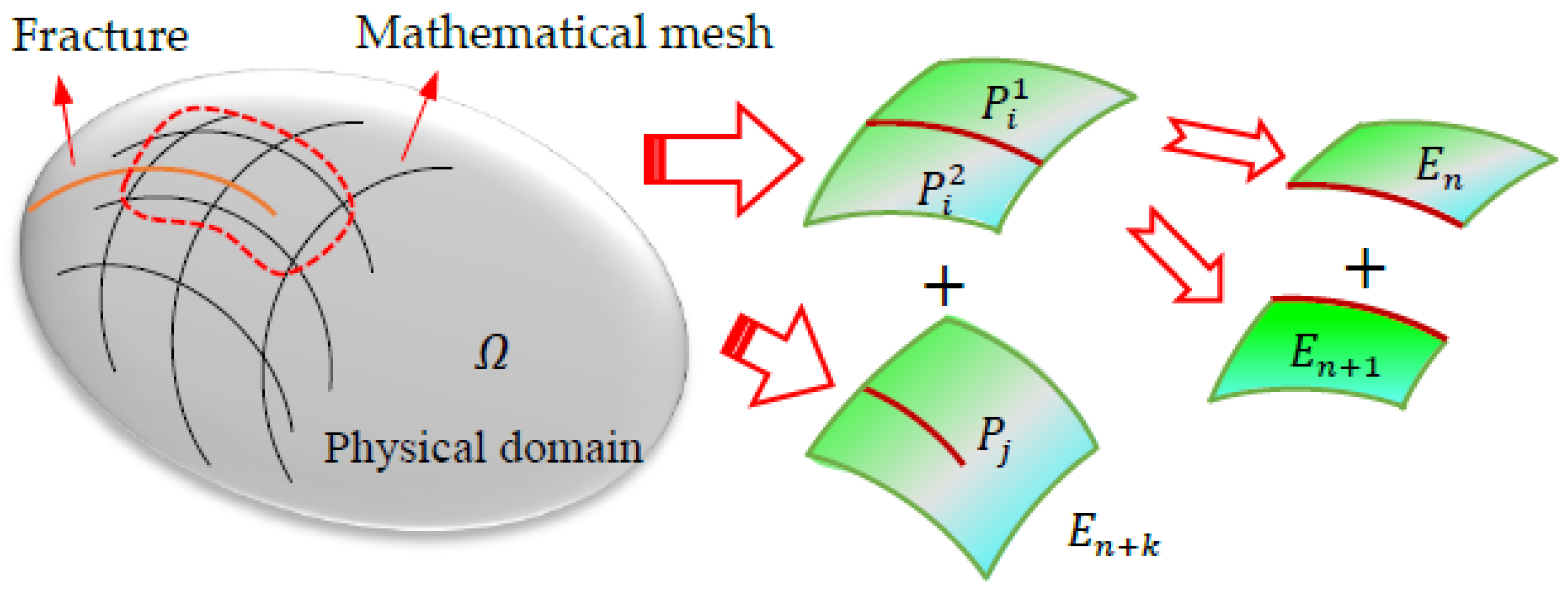
2.1. Fundamentals of the NMM

Traditional numerical methods use a single cover to mesh the physical domain, and each finite element and distinct element are associated with nodes or a physical boundary. In contrast to FEMs and DDA, NMM adopts a dual cover system containing a mathematical cover (MC) and physical cover (PC) to describe the physical domain [25,27,29,30,31]. In this sub-section, a brief introduction to NMM theory is presented by using the partition of unity (PU) function.
The dual cover system in the NMM is constructed by means of MCs and PCs. The MC consists of a collection of mathematical patches. Each mathematical patch is a simply connected domain. By dissecting one or several mathematical patches with the components of the problem domain—namely, the boundary, the material interface, the joint/fracture, and the crack—the physical patches are obtained. All these physical patches comprise the PCs. The overlapping region of several PCs forms a manifold element (ME). Figure 2 gives a brief illustration of a cover system employed in the NMM, and a sketch the construction procedure of the cover system. When a hypothetical physical domain, Ω , is used for modeling, the mathematical mesh covers the whole domain Ω , and the physical boundary and discontinuities (i.e., rock fractures/fissures, joints and cracks, etc.) divide the domain into many different PCs. As highlighted, inside the red dotted circle, three PCs, denoted by P i 1 , P i 2 and P j (subscripts i and j are the MC indices, respectively), are formed from the fracture intersecting with the MCs. Then, the NMM elements are built by these overlapping PCs: E n and E n + 1 are formed from P i 1 and P i 2 , and E n + k (subscripts n and k are the re-index of the updated MEs) is formed by P j .
On each regular PC, a polynomial function of order n is employed to construct a local approximation function:
u i ( x , y ) = p ( x , y ) T d i ( x , y )
where d i ( x , y ) is an array of unknown coefficients on P i , and p ( x , y ) is the matrix of polynomial bases. p ( x , y ) = { 1 } is the zero-order polynomial function; p ( x , y ) = { 1 , x , y } T is the first-order polynomial function; and p ( x , y ) = { 1 , x , y , x x , x y , y y } T is used for the second-order polynomial function. In this study, p ( x , y ) = { 1 } is adopted to avoid the linear dependence problem.
Since NMM is also a PU-based method [39,40,41], the global approximation on each ME can then be constructed by connecting the weight functions with the local approximation functions as:
u ( x , y ) = i = 1 n w i ( x , y )   u i ( x , y )
where n is the number of PCs for the ME and w i ( x , y ) is the weighting function, which satisfies:
w i ( x , y ) = 0 ,   ( x , y ) P i ;   1 w i ( x , y ) 1   a n d     w i ( x , y ) 1 , ( x , y ) P i
In the present study, a triangular mesh is used to construct the MC; thus, the shape function of a 3-node triangular patch is applied to construct the weight function, and the displacements of P i can be rewritten as:
u i ( x , y ) = j = 1 6 d i j ( x , y )
where d i j ( x , y ) denotes the degrees of freedom (DOFs) related to P i . Finally, the displacement for each ME can be expressed as:
u ( x , y ) = i = 1 3 w i ( x , y )   j = 1 6 d i j ( x , y )
Based on the minimum energy principle, the global equations of equilibrium are derived by taking the derivatives of the DOFs, which can be simplified as:
[ K ] [ D ] = { F }
where [ K ] is the coefficient sub-matrix and [ D ] and { F } are the DOF sub-vector and the loading vector. Assuming that a discrete system consists of n PCs, Equation (6b) can be re-expressed as:
[ K 11 K 21 K 31 K 12 K 13 K 22 K 32 K 23 K 33 K 1 n K 2 n K 3 n                       K n 1 K n 2 K n 3 K n n ] ( D 1 D 2 D 3 D n ) = { F 1 F 2 F 3 F n }
where D i , F i (i = 1, 2,…, n) are 6 × 1 sub-matrices and D i is the deformation variable of PC i; F i is the load distributed to PC i; and K i j (i, j = 1, 2,…, n) is a 6 × 6 sub-matrix related to the material itself (i.e., K i j , i = j ) or the contact between block i and j (i.e., K i j , i j ). Then, a simplex integration method is used to analytically evaluate the element matrices, and an implicit Newmark time integration scheme is adopted to compute each step deformation of the global system.

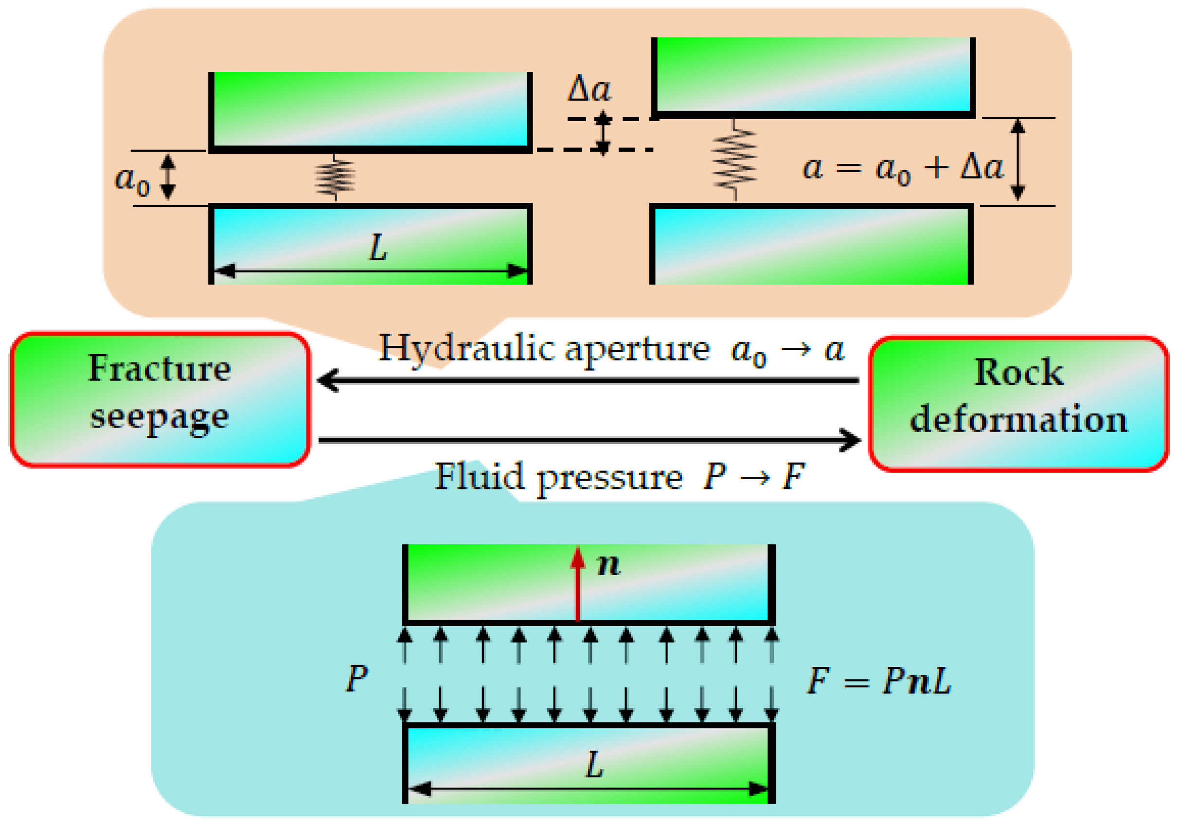
2.2. Basic Formulas of Seepage–Deformation Coupling Model

In this section, a coupled numerical model is implemented in which the fracture conductivity will be influenced by the mechanical deformation and, conversely, fluid pressure acting on the fracture interfaces will affect the mechanical deformation. As shown in Figure 1, the fluid pressure P F means the hydraulic force acting on the fracture surfaces leads to a change in the fracture aperture, such that a 0 a causes the fluid pressure. The incompatibility between constant strain field and general block shape was overcome by discretizations of deformable blocks. A residual flow method was introduced into the NMM so that unconfined flow problems with moving boundaries or free surfaces could be readily solved. For implementing the seepage–deformation coupling model into the NMM, the basic assumptions are:
  • The rock matrix is impermeable, and only fracture seepage is considered.
  • The fluid flow is assumed to be laminar, steady, viscous, and incompressible, and the fluid pressure is always positive.
  • The fluid flow has no effect on the strength of the material, and no hydraulic fractures initialize and propagate in the model.
Figure 3 shows a 2D example of a fracture network, in which the problem domain, dissected by six intersecting fractures, consists of eight independent blocks (i.e., denoted by numbers from to ⑧). Each block is constructed by several line segments and surrounded by a closed loop to model the contact and fluid flow in the NMM simulations. Resorting to the NMM mathematical meshing and physical meshes, each block is divided into a series of MEs (e.g., Ei in Figure 3); then, the block system, consisting of a fracture network and seepage paths, is established. In this way, the coupling between the fracture flow and deformation block is built. For example, the aperture between two connected blocks, denoted by ③ and ⑥, is filled with flowing fluid. The seepage path of 1–6 is divided into five small line segments by mathematical meshing, i.e., 1–2, 2–3, 3–4, 4–5, and 5–6, and each divided seepage path has two surfaces, which constitutes a fracture seepage element. Each coupled surface and separated seepage path is exactly a line segment of a loop belonging to blocks ③ and ⑥, respectively. Therefore, the closed loops are not only used to compute the contact forces but are also employed to generate the potential fracture network for calculating fluid flow. The simulations of seepage pressure in this study are based on the fracture coupling model, and the triangle meshing technique is employed to form MEs (e.g., E i in Figure 3) in the computations.
Considering a single planar fracture with an aperture of a, as shown in Figure 1, and taking into consideration that the flow is assumed to be laminar, the discharge through fractures can be expressed by Richard’s equation, i.e., the “cubic law”, to be:
q i j = a 3 g 12 μ i j = a 3 12 μ p i j L
where q i j is the flow rate of the seepage path with two end nodes i and j, i j is the hydraulic gradient, a and L are the aperture and length of the fracture, μ is the kinematic viscosity of fluid, and p i j is hydraulic pressure loss, which satisfies:
p i j = ( p j p i ) + ρ f g ( z j z i )
where p i and p j are the fluid pressure at nodes i and j, z i and z j are the piezometric heads at nodes i and j, respectively; ρ f is the density of fluid, and g is the acceleration of gravity. It can be deduced from Equation (9) that the flow rate can be calculated under a gravity effect when both fluid pressures are zero. Since Darcy’s law for fluid flow has been widely applied to simulate porous media [8,9,33], the “cubic law” can adequately compute fluid flow through the fracture network.
As discussed in [42], the flow rates of the nodes, related to the piezometric heads for an independent single fracture, are affected by saturation. Thus, to compute the flow rates of the fracture network, flow rates in Equation (8) are essentially multiplied by a parameter, f i s , which is a function of saturation, s i , satisfying 0   s i   1.
f i s = s i 2 ( 3 2 s i )
The total flow rate of node i can then be expressed as follows:
Q i = j = 1 N q i j
where N is the number of adjacent seepage paths around node i. It is found that the actual flow rate entering node j from node i will decrease if node i becomes unsaturated. Then, the flow rate between nodes i and j can be rewritten as:
q i j = f i s a 3 12 μ p i j L
Normally, the hydraulic aperture a referred to in Equation (12) is not constant, but changes with the element contact states and hydraulic pressures. The value of a can be assumed to be:
a = a 0 + a
where a 0 and a are the initial aperture and normal increment, respectively. As discussed in [43], the minimum and maximum values of the fracture aperture are prescribed as a m i n and a m a x , respectively. The expression of increment a can be written for both non-parallel fracture and ideal parallel fracture elements (as can be seen in Figure 4) as follows:
a = a a v e r 1 + r ( 16 r 2 1 + r ) 1 / 3
where a a v e r = ( a k + a k + 1 ) / 2 , r = a k / a k + 1 , a k is the relative distance between points k in the normal direction n, and a k + 1 is the relative distance between points k + 1 in the normal direction, as shown in Figure 5.
Figure 6 gives an example of a typical fracture network model in the NMM. Within a random time step, once the total flow rate Q 1 at node 1 is collected by the surrounding four connected seepage paths, the hydraulic pressure at node 1 can be calculated by Equation (11) (i.e., q 11 , q 12 , q 13 , q 14 in Figure 6). The new hydraulic pressure p i at node i can then be expressed as:
p i = p i 0 + k f Q i t A i k f A i A ¯ i
where p i 0 is the initial pressure at node i at the present time step, k f is the bulk modulus of the fluid, t is the time step size, and A i = A i A i 0 and A ¯ i = ( A i + A i 0 ) / 2 where A i 0 and A i are the initial and current areas that surround node i in the time step, respectively. In this study, the area of given node i is defined as half of the total area of all fracture paths connecting to the node. Thus, the area of node 1 as shown in Figure 6 can be obtained as:
A 1 = 1 2 j = 1 4 A 1 j = ( A 11 + A 12 + A 13 + A 14 ) / 2
where A 1 j , j = 1, 2, 3, 4 is the volume of seepage paths connecting node 1.
It is noted that if the fluid flow of node i is unsaturated, the value of the pressure p i in Equation (15) is assumed to be zero. Then, saturation s i can be expressed as:
s i = s i 0 + Q i t A i A i A ¯ i
where s i 0 is the initial saturation at the time step in node i. When s i satisfies the condition of s i 1 , pressure p i can be calculated by Equation (15), which ensures the conservation of fluid mass in the simulations. Thus, Equation (11) satisfies the principle of fluid mass conservation and can be rewritten as:
( j = 1 N q i j ) i + Q i 0
where Q i is the total external recharge (or discharge) rate.

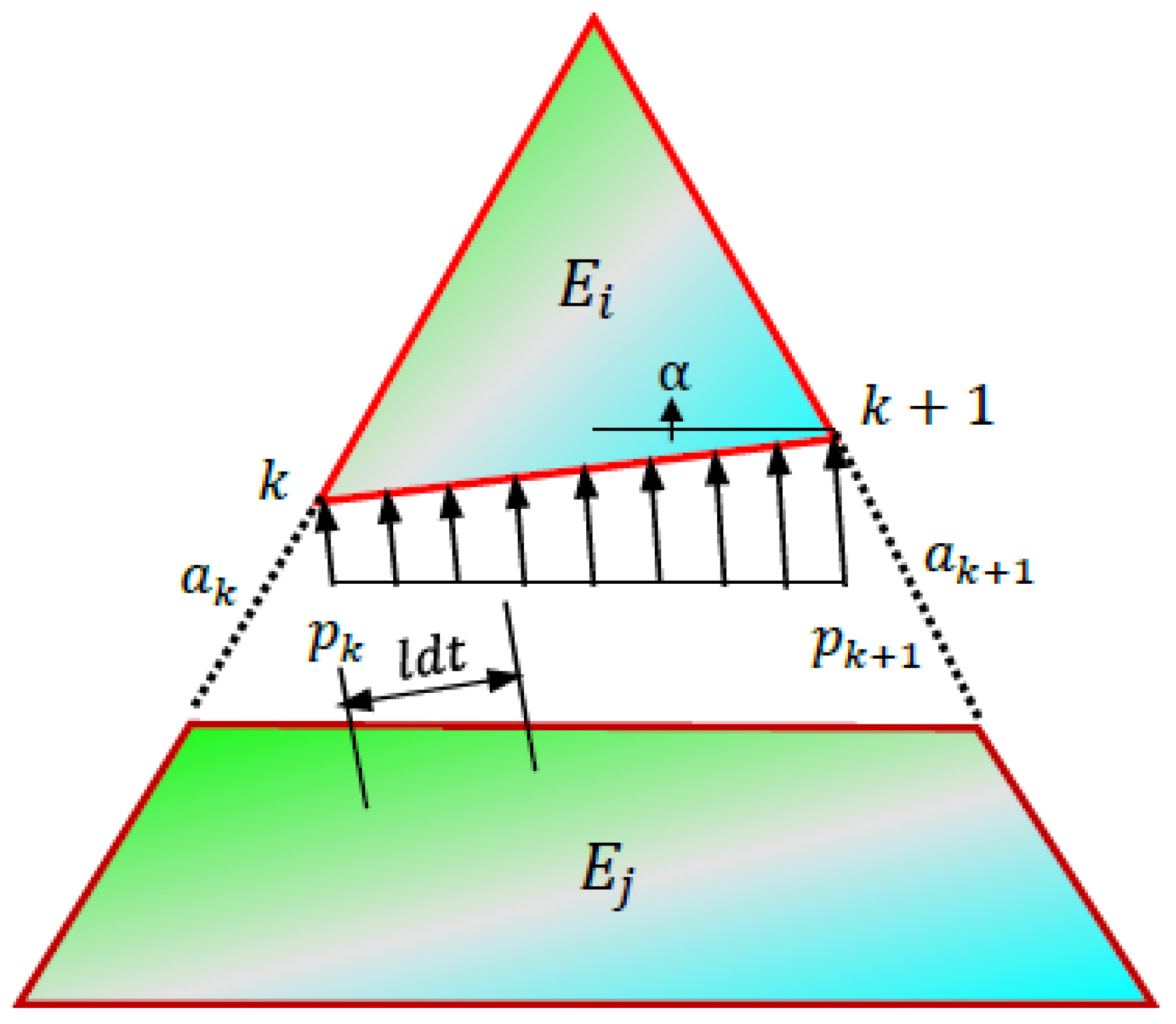
2.3. Fluid Pressure on Manifold Element Boundaries

Fluid flow in fractures imposes fluid pressure on the interface of the fractures, producing deformation of rock fractures and changing the fracture aperture and the hydraulic conductivity of the fracture element. Subsequently, the hydraulic heads will be redistributed in the flow network. In the present study, fluid pressure on the fracture element can be assumed as a linear distributed behavior. As shown in Figure 6, the fluid pressure is acting on the boundary of k ( k + 1 ) by the manifold element E i . If p k = ( p k x ,   p k y ) and p k + 1 = ( p ( k + 1 ) x ,   p ( k + 1 ) y ) are the fluid pressures acting on element E i , the coordinates of points k and ( k + 1 ) are ( x k ,   y k   ) and ( x k + 1 ,   y k + 1   ) , respectively. The fluid pressure at any point on the element boundary can be expressed as:
{ p x ( t ) = p k x + ( p ( k + 1 ) x p k x ) t p y ( t ) = p k y + ( p ( k + 1 ) y p k y ) t   ( 0 t 1 )
The potential energy of the linear distributed fluid pressure acting on the side of E i can be written as:
  l = 0 1 ( u ( t )   v ( t ) ) ( p x ( t ) p y ( t ) ) l d t
Substituting Equation (18) into Equation (19), the expression can be rewritten as:
  l = [ D i ] T 0 1 [ T i ] T ( p x ( t ) p y ( t ) ) l d t
in which [ D i ] and [ T i ] are the deformation matrix and displacement matrix of element E i , respectively. The length l of the element edge of E i is:
l = ( x k + 1 x k ) 2 + ( y k + 1 y k ) 2
To minimize the potential energy, the nodal load of element E i caused by distributed fluid pressure can be expressed as:
f i = Π l ( 0 ) d r i = d r i ( [ D i ] T 0 1 [ T i ] T ( p x ( t ) p y ( t ) ) l d t ) ,   r = 1 ,   2 ,   ,   6
in which f i is a 6 × 1 submatrix, which then is added into the global force vector [ F i ] as follows:
f i = 0 1 [ T i ] T ( p x ( t ) p y ( t ) ) l d t [ F i ] ,   r = 1 ,   2 ,   ,   6
Subsequently, such line loading is equivalent to two forces [ F i ] acting on the nodes of fracture elements, and Equation (23) can be then simplified to:
[ F i ] = ( T i ( x k , y k ) ) [ E ] { W k ( x k , y k ) } + ( T i ( x k + 1 , y k + 1 ) ) [ E ] { W k + 1 ( x k + 1 , y k + 1 ) }
where T i ( x k , y k ) is an interpolation polynomial for element E i [25], i.e., the weight function in an NMM or the shape function in a FEM; [ E ] is the hydraulic head matrix; and W k ( x k , y k )   is the weight matrix for line loading, expressed as follows:
{ T i ( x k , y k )               = ( w i ( x k , y k ) 0 0 w i ( x k , y k ) )   T i ( x k + 1 , y k + 1 ) = ( w i ( x k , y k ) 0 0 w i ( x k , y k ) )  
[ E ] = ( p k s i n α p k + 1 s i n α   p k c o s α   p k + 1 c o s α )
{ W k ( x k , y k ) = ( L 3 L 6 ) T W k + 1 ( x k + 1 , y k + 1 ) = ( L 6 L 3 ) T
where w i ( x k , y k ) and w i ( x k , y k ) are weight functions over element E i , L is the length of the fracture, and α is the angle between the element boundary and the x-axis.

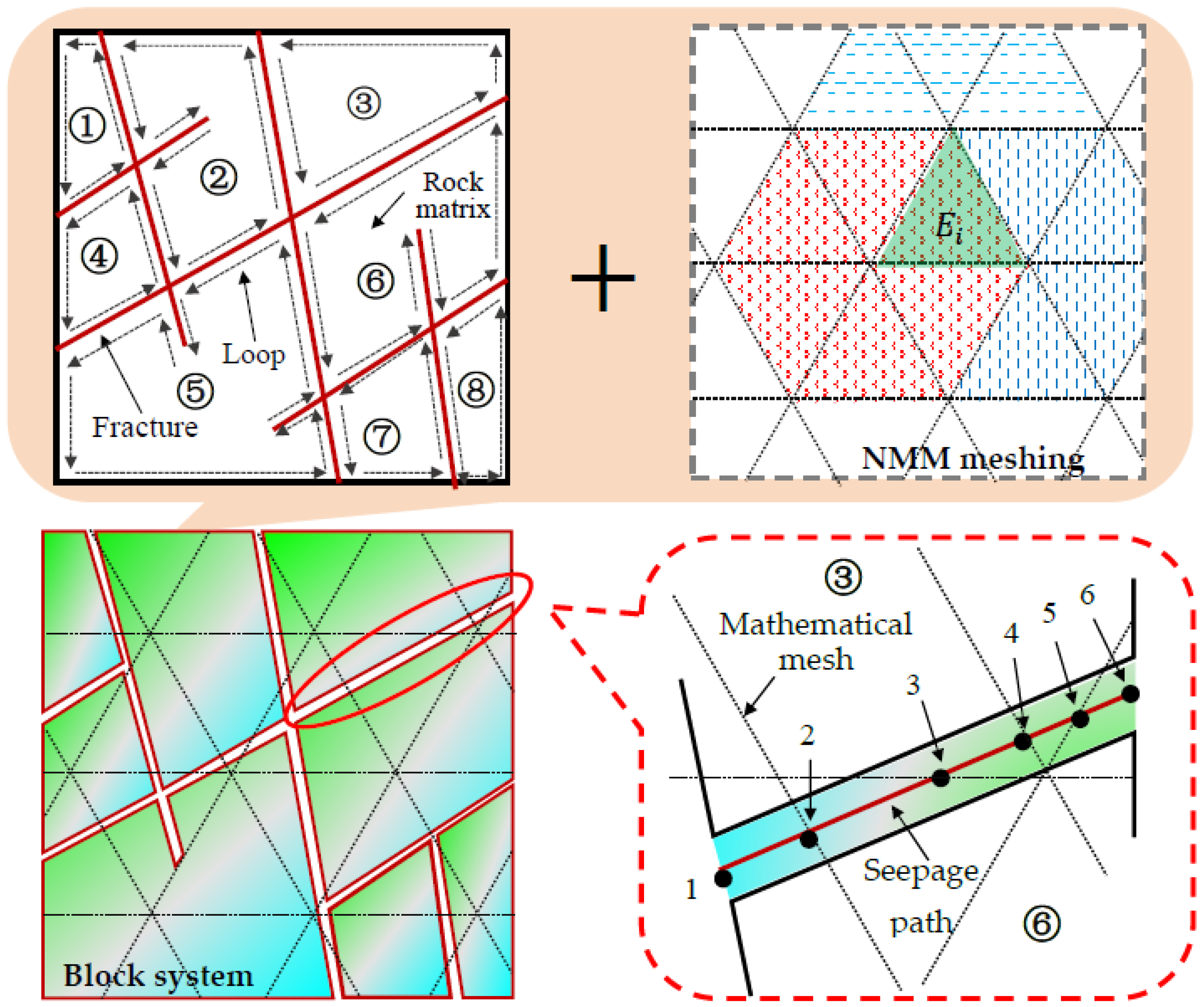
3. Modeling of Seepage along Fractured Network by the NMM

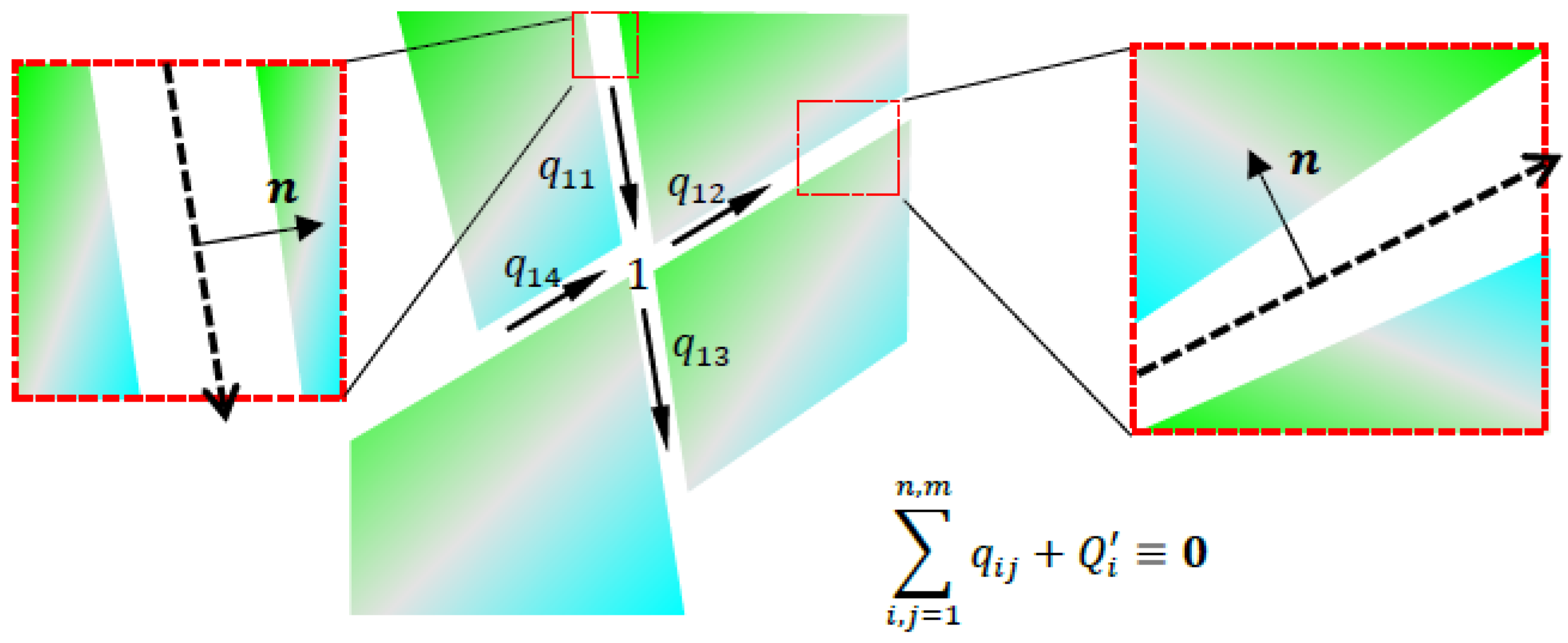
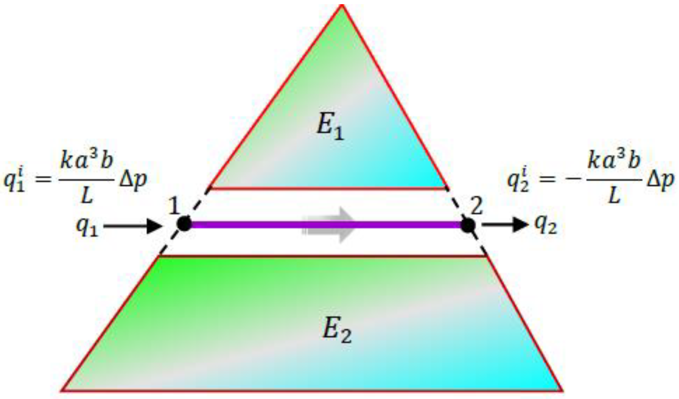
3.1. Calculation of Fluid Pressure along the Fracture Network

Although high normal contact acts on the fracture aperture of natural fractures, there is still a certain fracture width and/or mechanical gap to allow fluid flow through the fracture [44,45]. Based on the abovementioned theory of Darcy’s law of fluid flow in porous media and fracture networks, the “cubic law” applied in the present study can describe fluid flow through parallel and wedge fractures [46].
On implementation of the coupled seepage–deformation model, the piezometric head H is taken into consideration to push Darcy’s law, and flow rate q i can be re-expressed as:
q i = a 3 g 12 μ i = a 3 12 μ γ f H i L i = K A i H i L i
where K = a 2 γ f 12 μ is the fracture hydraulic conductivity, A i is the area of the fracture cross-section, H i is the piezometric head loss, and L i is the length of the fracture segment i. Then, the discharge at two end nodes of fluid element i can be obtained based on Equation (26), which is expressed as:
{ q 1 i q 2 i } = T i [   1 1 1   1 ] { H 1 i H 2 i }
where q 1 i and q 2 i are the nodal discharge vectors at end nodes 1 and 2 of the fluid element i, T i = γ f a 3 12 μ L i is the fracture characteristic matrix, and H 1 i and H 2 i are the nodal piezometric head vectors at nodes 1 and 2, respectively.
Take a simplified example of a fracture network as shown in Figure 7. Assuming Q 1 to be the element nodal 1 discharge, the total flow discharge of inflow or outflow at node 1 can be written as:
Q 1 = i = 1 N q 1 i
where N is the total number of element boundaries connected to node 1. Assembling all the element nodes to be positioned within the local seepage paths, the global equilibrium equations can be obtained as:
[ T ] { H } = { Q }
where [ T ] is the network characteristic matrix, { H } is the network piezometric head vector, and { Q } is the network flow vector. Then, a system of equilibrium equations from Equation (29) can be rewritten as:
[ T 11 T 21 T 31 T 12 T 13 T 22 T 32 T 23 T 33 T 1 n T 2 n T 3 n       T n 1 T n 2 T n 3 T n n ] { H 1 H 2 H 3 H n } = { Q 1 Q 2 Q 3 Q n }
Referring to Equation (30), the piezometric head, H i   ( i = 1 ,   2 , , n ) , at each fluid node can be obtained. Then, the fluid pressure   p i can be calculated from H i and the elevation head, h e = z i z d , as:
p i = γ f h p = γ f ( H i h e ) = γ f ( H i z i + z d )
where h p is the pressure head, z i is the vertical coordinate of the fracture node i, and z d is the vertical coordinate of the datum line.
It is noted that Equation (7) contains an unknown vector of Equation (30)—piezometric head { H } —while the coefficient matrix [ T ] of Equation (30) contains the unknown vector [ D ] of Equation (7). Therefore, the two equations are coupled. However, since the matrix [ T ] and the displacement vector [ D ] are not linear, Equations (7) and (30) can not be written as a unified formula and can only be solved by sequential iteration methods.

3.2. Calculation of Factor of Safety (FoS) along Rock Fractures

Normally, the stability of a rock slope has been evaluated by the global factor of safety (FoS), but real instability always starts from the most detrimental site. Therefore, rather than using the global FoS, if the local FoS can be applied, slope stability will be evaluated more accurately.
In the NMM simulations, discontinuities such as fractures/joints and weak interlayers between the fractured rock masses are modeled as a contact block, and a pair of normal and shear springs then connect the adjacent elements. A normal penalty function on the contact elements is then introduced. The stiffnesses of the shear spring is set as follows:
{ k n = l 2 E                                     k s = l 2 E 2 ( 1 + ν ) = l 2 G
where k n and k s are the normal and shear spring stiffness, E and G are the Young’s and shear modulus, ν is Poisson’s ratio, and l is the length of the contact edge.
Assuming that a continuous edge is divided into M segments, the normal and shear forces on 2 M segments can be calculated correspondingly. Thus, the contact force acting on the ith edge (i.e., i ( 0 ,   M ] ) between two contact elements can be expressed as the following:
σ i 1 = 2 k n i d n i 1 l ,   σ i 2 = 2 k n i d n i 2 l   τ i 1 = 2 k s i d n i 1 l ,   τ i 2 = 2 k s i d n i 2 l }
where σ i 1 , σ i 2 and τ i 1 , τ i 2 are the normal and shear contact stresses from edge i to i + 1 and d n i 1 and d n i 2 are normal and shear deformation of the contact springs, respectively.
The local shear and tensile FoS between contact elements can be calculated as follows:
{ F o S i j = f i k n i d n i j + τ 0 i l i / 2 k s i d s i j F o S i j = 2 T 0 i k n i ( d n i 1 + d n i 2 )     ( i = 1 ,   2 ,   , M ; j = 1 ,   2 )
where F o S i j and F o S i j are the local shear and tensile FoS, respectively. The global shear FoS can be then obtained as:
F o S = i = 1 M [ f i k n i ( d n i 1 + d n i 2 ) + f i k n i d n i j + τ 0 i l 2 ] i = 1 M k s i ( d s i 1 + d s i 2 )
where f i and τ 0 i are the friction coefficient and cohesion of the ith contact pair and T 0 i is the tensile strength of ith contact segment.

4. Numerical Examples

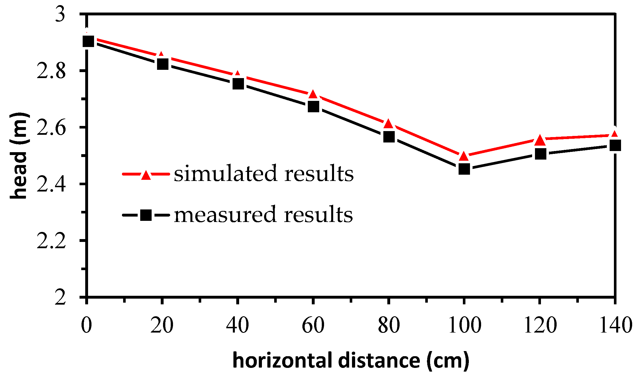
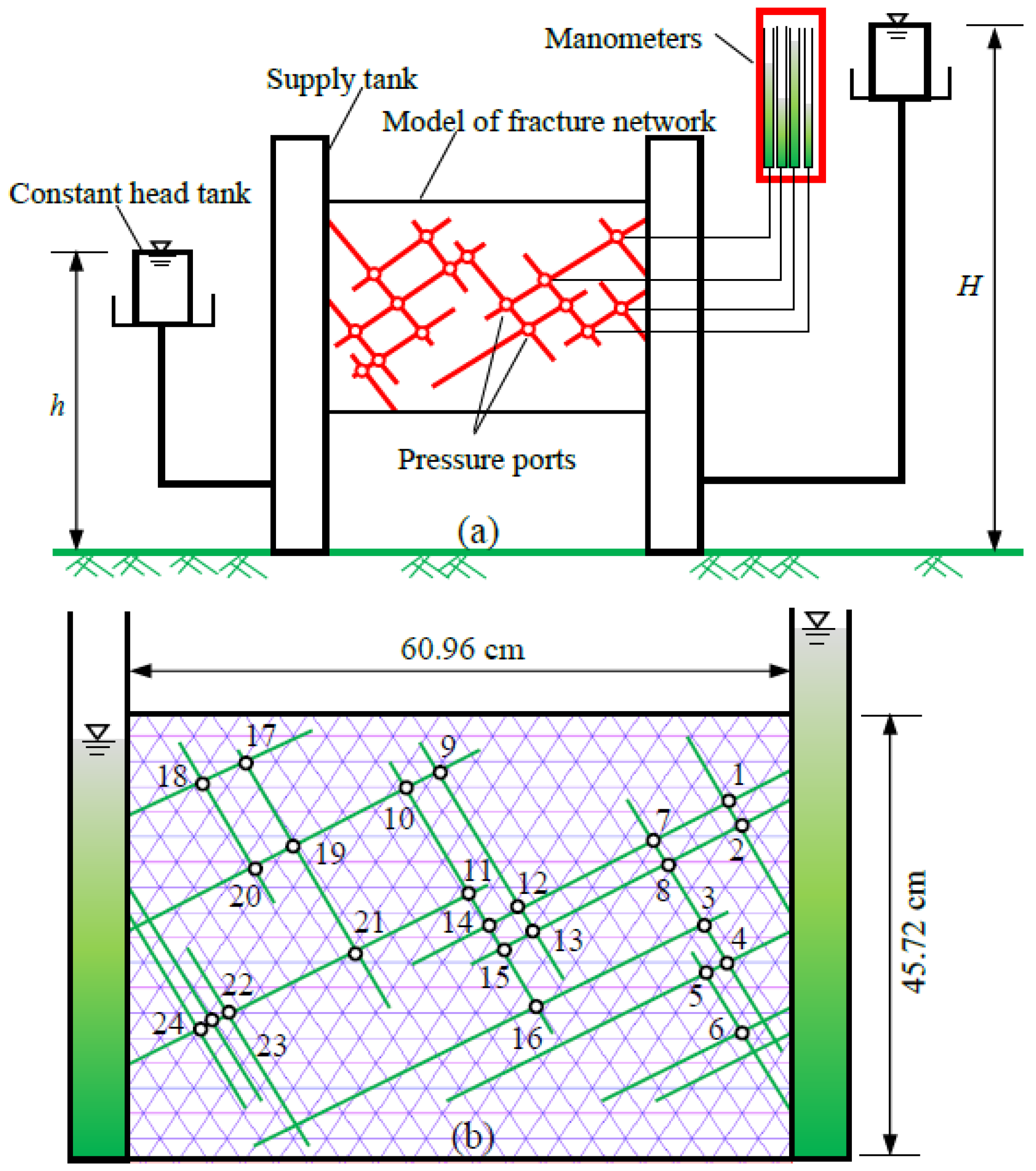
4.1. Verification of the Coupled Seepage–Deformation Model

Firstly, to verify the proposed coupled model for the NMM, a 2D flow in a homogeneous aquifer is studied. As can be seen from Figure 8, the length of the model is L and the prescribed water heads are h1 and h2. The bottom boundary of the model is assumed to be impermeable (i.e., q = 0). The analytical solution of the total discharge for this model is [47]:
Q = k h 1 2 h 2 2 2 L
in which Q is the total discharge and k is the permeability coefficient.
As shown in Figure 9, a 2D model of a fracture system consisting of constant fracture spacing S and aperture a is taken into consideration. The average velocity of fluid flow in an equivalent porous medium can be calculated using Darcy’s Law as follows:
v = q S = ( a 3 p 12 μ L ) / S = ρ f g a 3 12 μ L h S
where q is the flow rate through a divided fracture with length S. As the hydraulic gradient i = h / L can be described directly, the equivalent permeability coefficient for the model can be obtained as:
k = a 3 12 μ ρ f g S
Thus, the final discharge can then be expressed as:
Q = a 3 12 μ ρ f g S h 1 2 h 2 2 2 L
In the simulations, a discretized model by the NMM as plotted in Figure 9 is established in which two sets of parallel fractures are distributed throughout the homogenous mass with the prescribed geometric dimensions of a = 0.1 mm, S = 0.5 m, L = 8.0 m, h 1 = 4.0 m, and h 2 = 1.0 m. The input physical parameters applied into the model are as follows: the unit weight is 25.5 kN/m3, Young’s modulus is 75 GPa, Poisson’s ratio is 0.22, fluid viscosity coefficient is 1.005 × 10 3 Pa s, cohesion of the fracture is 0.1 MPa/m2, friction angle is 25°, and the normal contact stiffness is 200 GPa. To obtain computational accuracy, a constant time step, t , 5 × 10⁻⁸ s is applied. In the model, a total of 2800 PCs, 3688 MEs, and 128 flow segments are obtained, and 7 measured points are prescribed to sum the discharge of the fracture network system. The total discharge can then be written as:
Q = i = 1 7 Q i
Finally, the total discharge calculated by the analytical equation of Equation (40) is:
Q = 1.563 × 10 6   m 3 / s
The total discharge simulated by the NMM is:
Q = i = 1 7 Q i = ( 0 + 0.706 + 0.631 + 0.143 + 0 + 0 + 0 ) × 10 6 =   1.480 × 10 6 m 3 / s
Comparing the analytical solution to Equation (39), one can see that the relative error of the NMM simulation is only 5.31%. It is seen that the simulated results using the proposed coupled model agree well with the analytical solution.

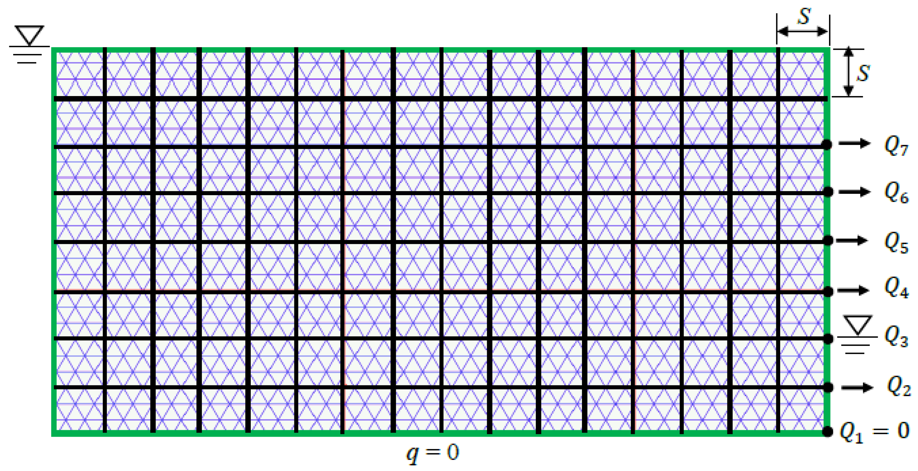
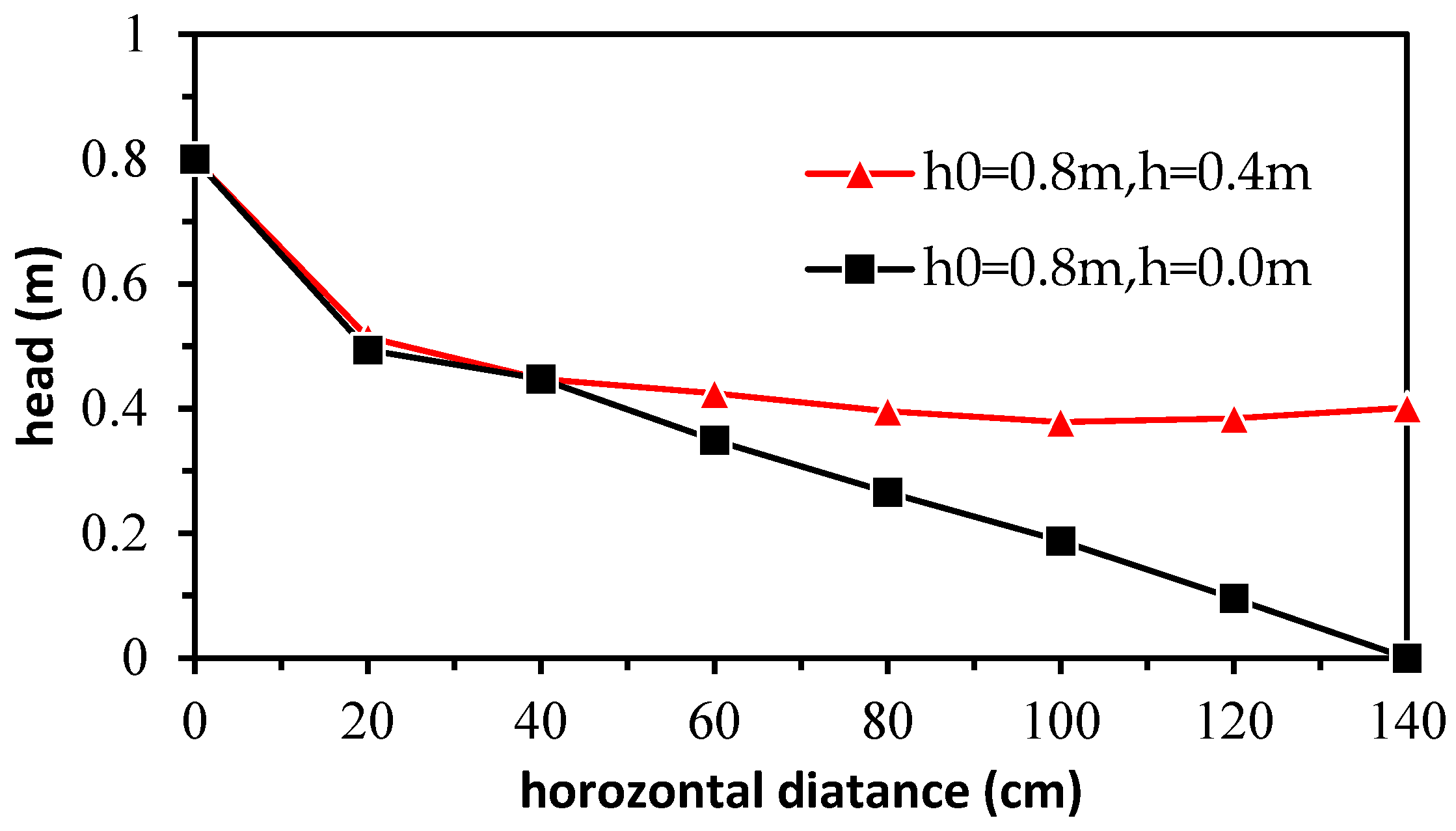
4.2. Fracture Seepage of Fluid Flow through a Regular Fracture Network

The verification of this example focuses on the developed fluid flow algorithm based on the coupled seepage–deformation model for determining the position of the phreatic surface. As referred to in [21,48], an earlier experiment of water flow through a regular fracture network is conducted in which the fracture system consists of two perpendicular sets of parallel fractures, and 28 stacking blocks with uniform spacing of h = 0.2 m are assembled (as seen in Figure 10). To simulate the pressure head distribution of the phreatic surface along the bottom of impermeable boundaries, the fractures are prescribed a uniform aperture, a, of 0.4 mm; the hydraulic boundary conditions used in the NMM are listed as follows: a constant water head, h, of 2.9 m is assigned to the left side of the model, a constant velocity of 50 cm/s at the lower-right corner is prescribed, and there is no flow rate for the other boundaries.
A comparison of the measured and simulated results of the water head along the base of the model is plotted in Figure 11, and the simulated results (denoted by the red line) agree well with the results (presented by the black line) measured by the experiments.
Following the aforementioned fracture network (i.e., see Figure 11), two assumptions are carried out here by changing the hydraulic boundary conditions as follows:
  • h0 = 0.8 m is prescribed at the left side of the model, and except for the impermeable base, the other boundaries are free surfaces;
  • h0 = 0.8 m is prescribed at the left side of the model, but the right side has a water head of h = 0.4 m.
The simulated results of the phreatic surfaces using the proposed flow algorithm for the above two assumptions are plotted in Figure 12. The simulated results of assumptions of h0 = 0.8, h = 0.4 (denoted by the red line and bar charts) and h0 = 0.8, h = 0.0 (plotted by the black line) agree well with the experiment [48], which achieves the expectation to the fracture model and further verifies the proposed seepage–deformation model.

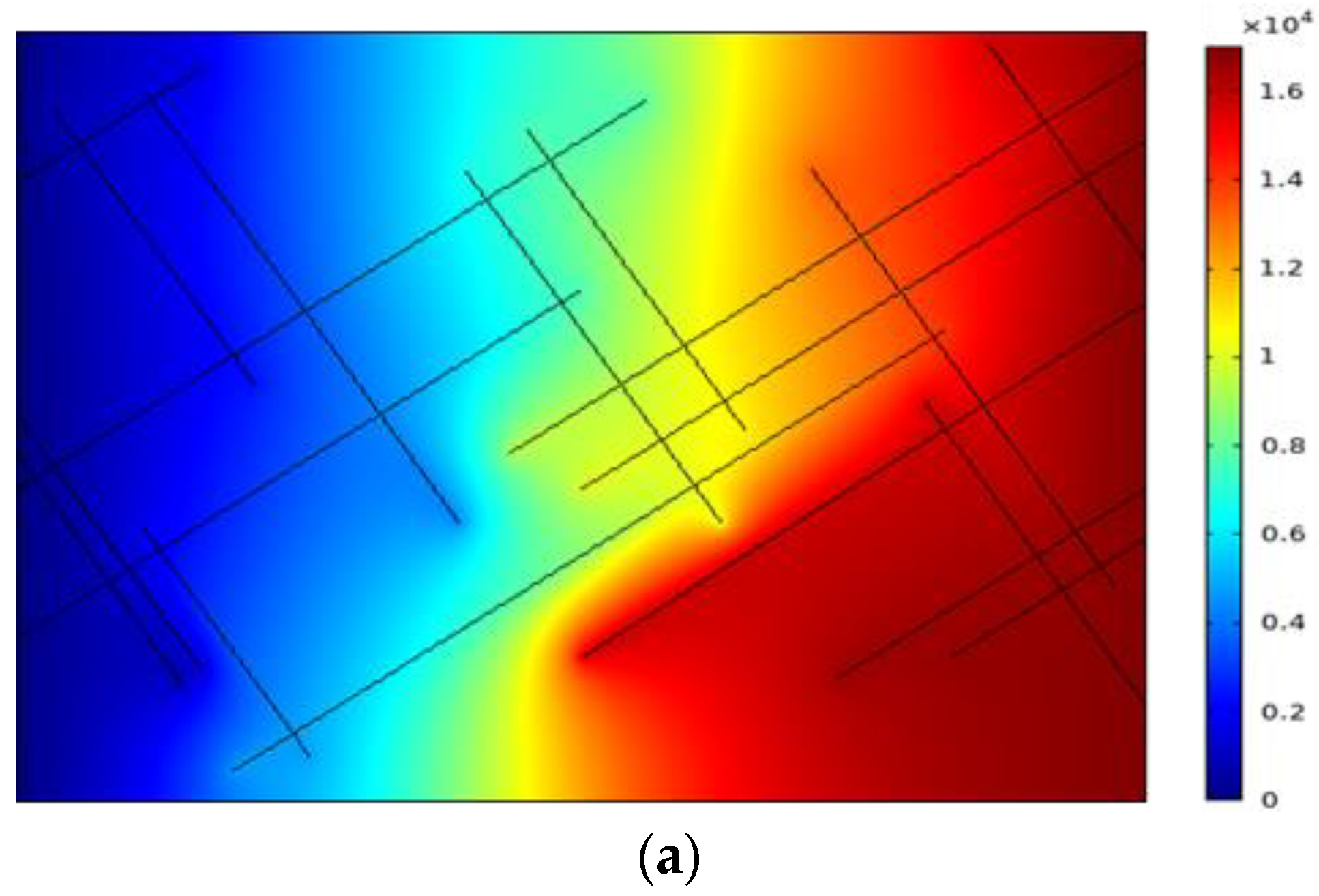
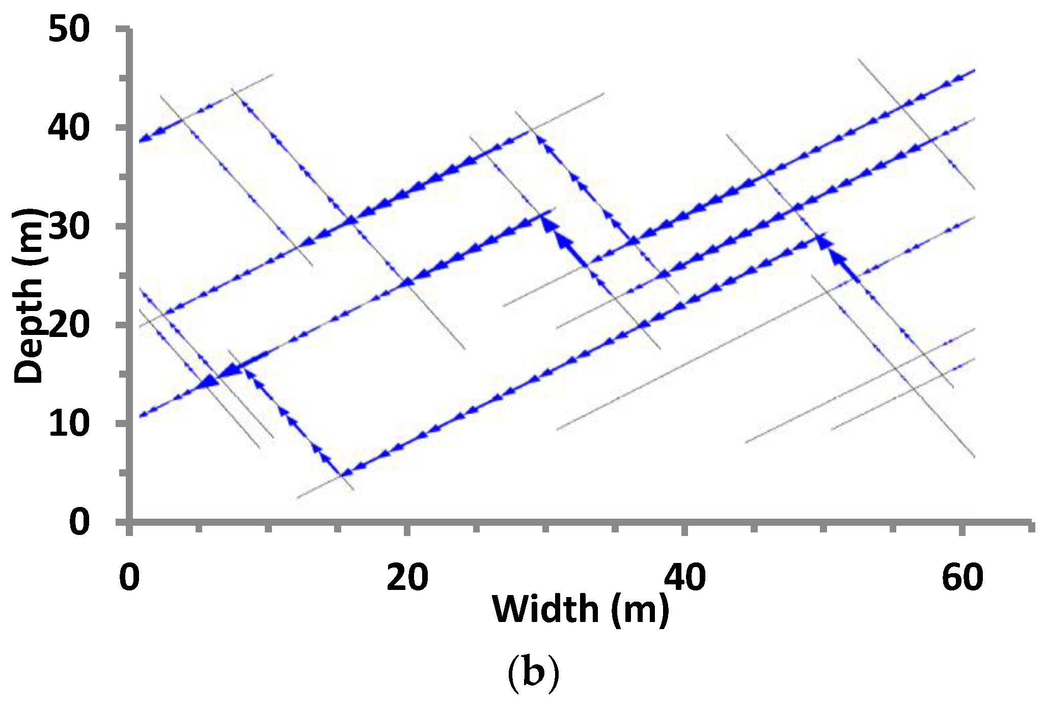
4.3. Joint Seepage in an Arbitrary Complex Rock Fracture Network

To further validate the coupled seepage–deformation algorithm, a steady-state flow problem in a complex fracture network is simulated, and comparison with the experimental results as referred to in [49] is then carried out to check the proposed method. As shown in Figure 13, a schematic of the complete laboratory device is illustrated, and a physical experimental model to simulate 2D flow through jointed fractures is then constructed. The depth and width of the model are assumed to be 45.72 cm and 60.96 cm, respectively.
In the present study, hydraulic pressure is simulated at 24 joint intersection ports according to the previous four typical tests in [48] (T1–7 to T1–10) (as listed in Table 1) subjected to a hydraulic gradient i = h / L ranging between 0.01 and 2.84 and corresponding head differential h = H h from 0.762 cm to 172.84 cm. The physical input parameters are the following: the unit weight is 25.0 kN/m3, Young’s Modulus is 3.1 GPa, Poisson’s ratio is 0.35, and the kinematic viscosity of water is 1.005 × 10⁻³ Pa s. Four representative tests (T1–7 to T1–10) are analyzed by the NMM, and the simulated results are listed in Table 2, in which the errors in head value, Er, at each measured port are expressed as:
E r = h l h n H h
where h l is the experimental head value, h n is the value simulated by the NMM, H is the upstream head, and h is the downstream head. For each test, the average error in head value, E ¯ a r , can be obtained as:
E ¯ a r = 1 n n | E r |
where n ( n = 24) is the number of measured ports. Values of E ¯ a r are assembled from Table 2. It is found that the simulated results indicate that E ¯ a r is not more than 3.53% and increases with the increasing hydraulic gradient.
The pressure and flow rate distributions of the fractures are calculated by the NMM. As shown in Figure 14, the calculated hydraulic pressure with rock matrix permeability (e.g., 1.0 × 10⁻¹⁴ m2) by FEM code indicates the pressure distribution when porous media is considered (Figure 14a), but the simulated results using the proposed model (Figure 15b) by the NMM agree very well with both the hydraulic pressures and the flow rates at the measured ports. It is clear that the proposed seepage–deformation model is more efficient and flexible for simulating steady-state fluid flow in discrete fracture networks.

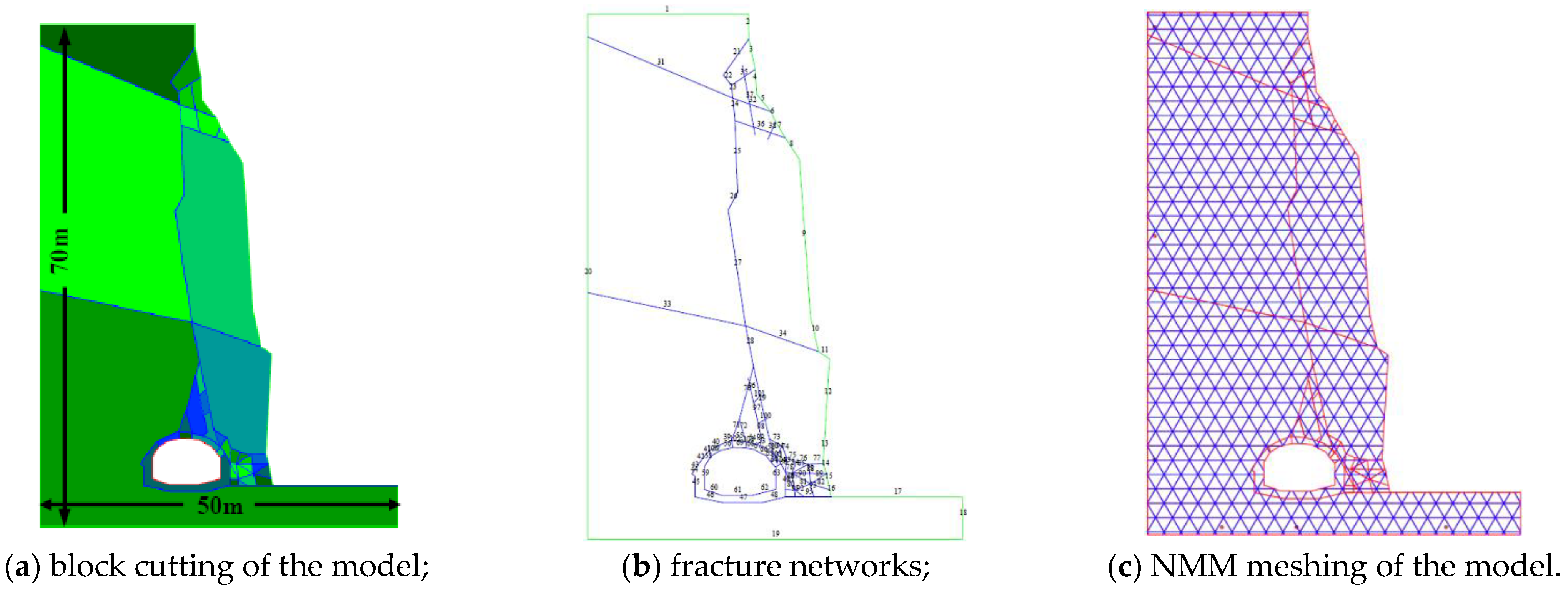
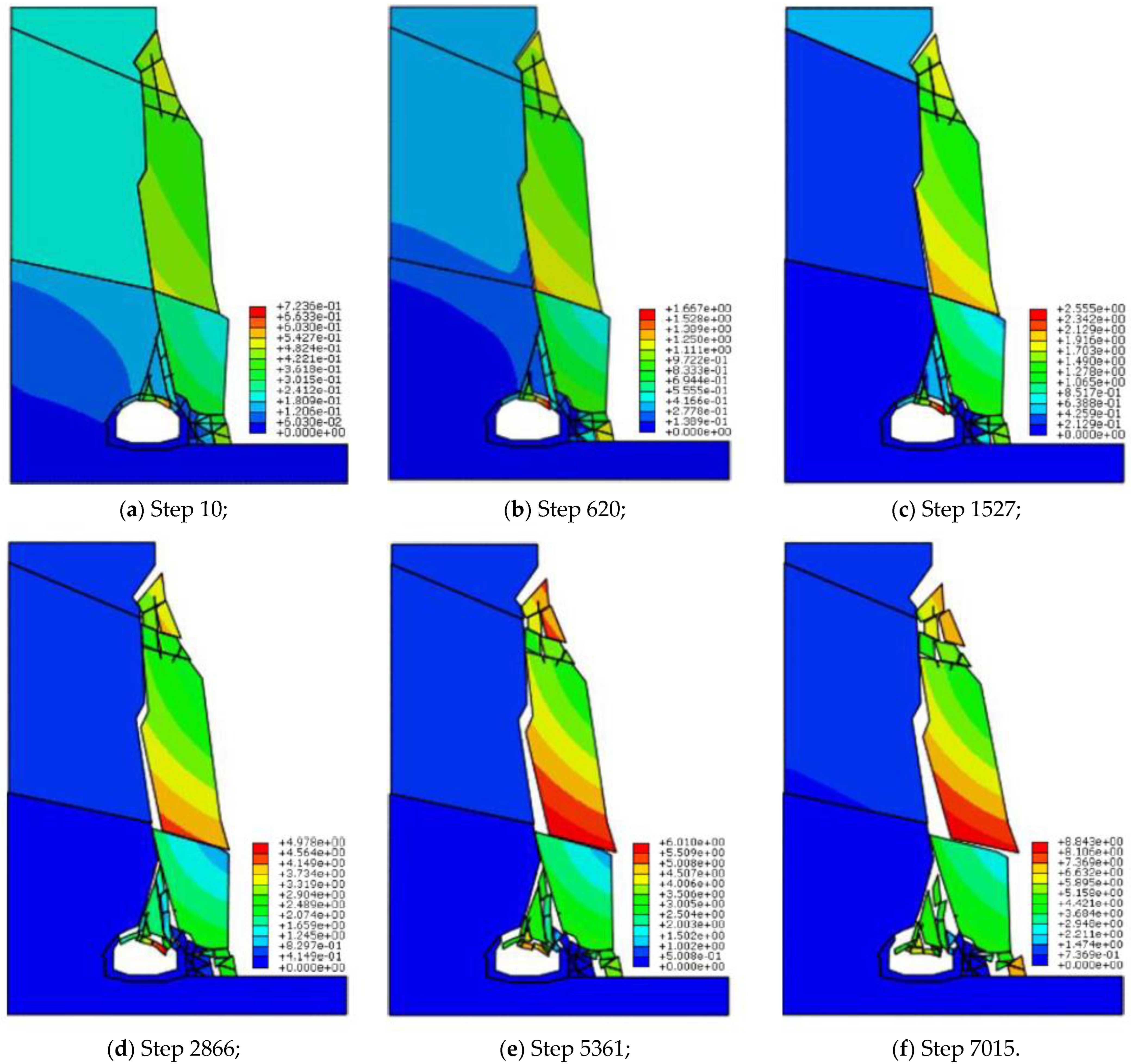
4.4. Rock Slope Stability Analysis Using the Coupled Seepage–Deformation Model

In this study, the proposed seepage–deformation model by the NMM method is used to simulate the failure process of a rock slope with a tunnel and to calculate FoS considering the effects of fracture flow on the rock masses. As shown in Figure 15, the NMM model consists of rock blocks and fracture networks containing both the existing fractures and virtual/potential fractures. The height and width of the slope are selected as 70 m and 50 m, respectively. A total of 1427 PCs, 2053 MEs, and 46 flow segments are obtained, and 208 measured points are prescribed to calculate the fluid flow rates of the fracture network system. The aforementioned fracture network is taken as a seepage path, and the strengths of potential failure features are considered as being equal to those of the intact rock mass. The division of blocks is investigated after a collapse disaster [50,51]. The input parameters, based on the investigation and experimental results, are listed in Table 3.
According to the expected failure mode, the main persistent fracture from the crest of the slope to the lower tunnel (see Figure 15) is taken as the possible sliding surface, and the local FoS, distributing along the sliding surface, is calculated under the following three considered cases:
  • The effect of groundwater is ignored, and only the self-weight of the rock mass is considered (i.e., Condition 1);
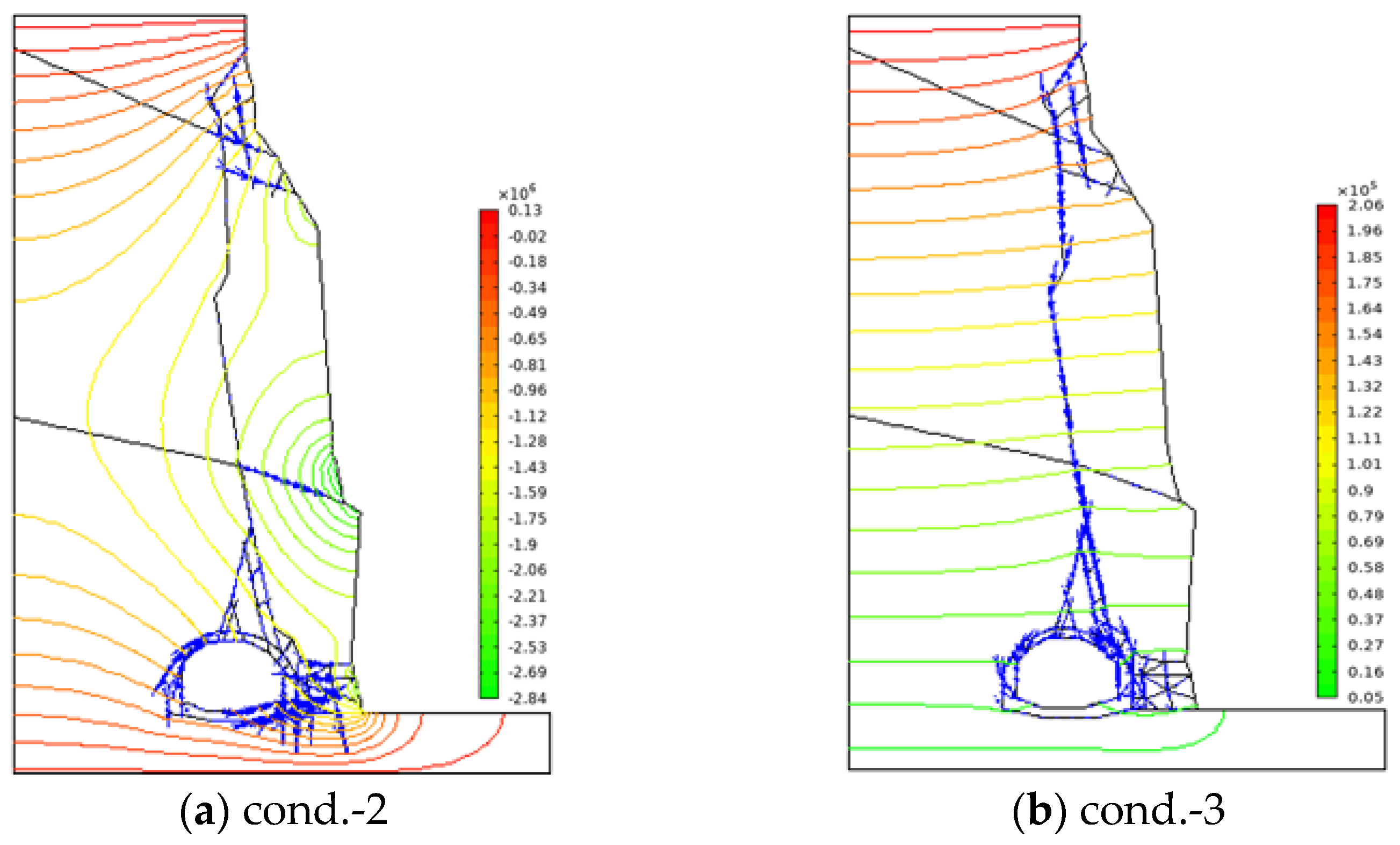
  • The effect of groundwater is not ignored, the highest groundwater head is located at the top of the slope (see Figure 15), and the bottom of the slope is taken as an outlet for the water flow (i.e., Condition 2);
  • The highest groundwater head is the same as Condition 2, but considering the condition under a frozen state of the rock slope surface, the groundwater outlet is blocked (i.e., Condition 3).
The local FoS can be calculated by Equation (36), and the distribution of the local FoS along the main sliding surface under the three prescribed conditions is plotted in Figure 16. It can be seen that each local FoS represents the typical stability state of a segment of sliding surface (i.e., l/2 in Equation (33)). When the effect of fracture flow is not considered under Condition 1, the FoS of the other parts is greater than 4.0, except for the FoS of 3.95 near an elevation of 26.37 m (see Figure 16). This shows that the slope is stable without considering groundwater.
When Condition 2 is considered, the water flow and pressure head of groundwater along the fracture are shown in Figure 17a. It can be seen that the groundwater flows out from the outlet points on the slope, which shows that the water flow calculated by the NMM is reasonable. Although the drainage of the slope is considered, there is still high water pressure in the top segment, which causes a large tensile stress of 0.833 MPa near an elevation of 45.2 m (see Figure 16). Therefore, the local FoS at the top segment of the main fracture is declined dramatically, and the minimum FoS decreases to 1.26 to approach the limit equilibrium state. On the contrary, under Condition 3 (see Figure 17b), the groundwater cannot flow out along the rock slope surfaces, and the hydraulic pressure is equal to the difference between the highest water head and the elevation of each segment (i.e., h = h z ). Then, near the bottom of the slopes, the pressure head is greater, which decreases the local FoS along the whole sliding surface (see Figure 16). However, the minimum FoS still appears at the top of the slope, as the open fracture is less than 1.0, which creates the instability of the slope.
Due to the persistent effects of water pressure, once the fracture/crack expands downward, it will lead to the instability of the whole slope. Figure 18 shows the failure process simulated by the NMM using the proposed seepage–deformation algorithm. When the top segment of the fracture begins to expand, it rapidly penetrates the whole sliding surface and leads to the failure of other potential fractures (see Figure 18b). When the rock mass outside the sliding surface slides downward, the rock mass surrounding the tunnel (e.g., the triangular parts) falls, all the weight acts on the tunnel and the tunnel is crushed (see Figure 18c,d), and finally, complete failure occurs as shown in Figure 18e,f.

5. Conclusions

In the stability analysis of a rock slope, the effects of groundwater in rock fractures can not be neglected, as seepage and groundwater flow in the fracture network reduces the normal and shear effective stresses between the fractures and ultimately results in failure of the slope. In the present study, the coupling effects of fracture seepage, hydraulic pressures, and rock deformation are taken into consideration in the framework of the NMM. A coupled seepage–deformation model is developed to fully reveal the effects of fracture flow on the stability of a rock slope. To validate the ability of the proposed numerical model, three numerical examples of discharge through a homogeneous aquifer, fracture seepage of fluid flow through a regular fracture network, and joint seepage in a complex rock fracture network are simulated, in which the relative error of the NMM simulation is only 5.31% for the homogeneous aquifer simulations, and the calculated value of E ¯ a r is not more than 3.53% of the experimental results as referred to in [49]. The simulated results agree well with the analytical and/or experimental ones, which suggests the robustness and effectiveness of the proposed coupled seepage–deformation model. To further check the proposed seepage NMM model, the failure process of a rock slope with a tunnel is simulated and the local FoS of the model with and without considering groundwater effects are computed. The calculated minimum FoS approaches less than 1.0. The simulated results show that fracture hydraulic pressure is the direct cause of slope failure. The stability analysis results of the FoS are consistent with those of in situ investigations. Furthermore, the tunnel collapse and failure of the rock slope in different stages are reproduced. It shows that the proposed method can not only simulate the coupling effect of fracture seepage and rock mass deformation but also simulate the failure process of a rock mass system.

Author Contributions

Conceptualization, X.Q., Y.Z., Y.C. (Youran Chen), C.Q., E.P. and A.D.; Methodology, X.Q., Y.Z., Y.C. (Youran Chen), Y.C. (Youyang Chen), C.Q., E.P. and A.D.; Software, X.Q., Y.Z., Y.C. (Youyang Chen), C.Q., E.P. and A.D.; Validation, X.Q., Y.Z., C.Q., E.P. and A.D.; Formal analysis, X.Q., Y.Z., Y.C. (Youyang Chen), C.Q., E.P. and A.D.; Investigation, X.Q., C.Q., E.P. and A.D.; Resources, X.Q., Y.Z., C.Q., E.P. and A.D.; Data curation, X.Q., Y.Z., C.Q., E.P. and A.D.; Writing—original draft, X.Q., Y.Z., Y.C. (Youran Chen), Y.C. (Youyang Chen), C.Q., E.P. and A.D.; Writing—review & editing, X.Q., Y.Z., Y.C. (Youran Chen), C.Q., E.P. and A.D.; Visualization, X.Q., Y.Z., C.Q., E.P. and A.D.; Supervision, X.Q., C.Q., E.P. and A.D.; Project administration, X.Q., C.Q., E.P. and A.D.; Funding acquisition, X.Q., C.Q. and E.P. All authors have read and agreed to the published version of the manuscript.

Funding

The authors acknowledge support from the National Natural Science Foundation of China (Grant Nos. 51708016, 51774018 and 41877270), the Program of the State Key Laboratory of Coal Resources and Safe Mining (Grant No. SKLCRSM17KFA01), and EP and AVD acknowledge the support from the Australian Research Council through project DP190103260.

Conflicts of Interest

The authors declare no conflict of interest.

References

  1. Neuman, S.P. Trends, prospects and challenges in quantifying flow and transport through fractured rocks. Hydrogeol. J. 2005, 13, 124–147. [Google Scholar] [CrossRef]
  2. An, X.M.; Ning, Y.J.; Ma, G.W.; He, L. Modeling progressive failures in rock slopes with non-persistent joints using the numerical manifold method. Int. J. Numer. Anal. Methods Geomech. 2014, 38, 679–701. [Google Scholar] [CrossRef]
  3. Kim, Y.I.; Amadei, B.; Pan, E. Modeling the effect of water, excavation sequence and rock reinforcement with discontinuous deformation analysis. Int. J. Rock Mech. Min. Sci. 1999, 36, 949–970. [Google Scholar] [CrossRef]
  4. Barton, N.; Bandis, S.; Bakhtar, K. Strength, deformation and conductivity coupling of rock joints. Int. J. Rock Mech. Min. Sci. 1985, 22, 121–140. [Google Scholar] [CrossRef]
  5. Louis, C.A. A study of groundwater flow in jointed rock and its influence on the stability of rock mass. Rock Mech. Res. Rep. 1969, 10, 10–15. [Google Scholar]
  6. Japan Society of Civil Engineering. Report of Stability Analysis and Field Measurements for Rock Slope in Japan; Japan Society of Civil Engineering: Tokyo, Japan, 1994. [Google Scholar]
  7. Pal, S.; Kaynia, A.M.; Bhasin, R.K.; Paul, D.K. Earthquake stability analysis of rock slopes: A case study. Rock Mech. Rock Eng. 2012, 45, 205–215. [Google Scholar] [CrossRef]
  8. Biot, M.A. General solutions of the equations of elasticity and consolidation for a porous material. J. Appl. Mech. 1956, 78, 91–96. [Google Scholar] [CrossRef]
  9. Rice, J.R.; Cleary, M.P. Some basic stress diffusion solutions for fluid-saturated elastic porous-media with compressible constituents. Rev. Geophys. 1976, 14, 227–241. [Google Scholar] [CrossRef]
  10. Curran, J.H.; Carvalho, J.L. A Displacement Discontinuity Model for Fluid-saturated Porous Media. In Proceedings of the 6th ISRM Congress, Montreal, QC, Canada, 30 August–3 September 1987. [Google Scholar]
  11. Carvalho, J.L. Poroelastic Effects and Influence of Material Interfaces on Hydraulic Fracturing. Ph.D. Thesis, University of Toronto, Toronto, ON, Canada, 1990. [Google Scholar]
  12. Long, J.C.; Pemer, J.S.; Wilson, C.R. Porous media equivalents for networks of discontinuous fractures. Water Resour. Res. 1982, 18, 645–658. [Google Scholar] [CrossRef] [Green Version]
  13. Nouri, A.; Panah, A.K.; Pak, A.; Vaziri, H.; Islam, M.R. Evaluation of hydraulic fracturing pressure in a porous medium by using the finite element method. Energy Resour. 2002, 24, 715–724. [Google Scholar] [CrossRef]
  14. Wang, F.T.; Liu, Y. A mechanism-based simulation algorithm for crack propagation in non-uniform geomaterials. Comput. Geotech. 2022, 151, 104994. [Google Scholar] [CrossRef]
  15. Santillán, D.; Juanes, R.; Cueto-Felgueroso, L. Phase field model of fluid-driven fracture in elastic media: Immersed-fracture formulation and validation with analytical solutions. J. Geophys. Res. Solid Earth 2017, 122, 2565–2589. [Google Scholar] [CrossRef] [Green Version]
  16. Santillán, D.; Juanes, R.; Cueto-Felgueroso, L. Phase Field Model of Hydraulic Fracturing in Poroelastic Media: Fracture Propagation, Arrest, and Branching Under Fluid Injection and Extraction. J. Geophys. Res. Solid Earth 2018, 123, 2127–2155. [Google Scholar] [CrossRef] [Green Version]
  17. Jing, L.R.; Hudson, J.A. Numerical methods in rock mechanics. Int. J. Rock Mech. Min. Sci. 2002, 39, 409–427. [Google Scholar] [CrossRef]
  18. Cundall, P.A.; Strack, O.D.L. A discrete numerical model for granular assemblies. Geotechnique 1979, 29, 47–65. [Google Scholar] [CrossRef]
  19. Shimizu, H.; Murata, S.; Ishida, T. The distinct element analysis for hydraulic fracturing in hard rock considering fluid viscosity and particle size distribution. Int. J. Rock Mech. Min. Sci. 2011, 48, 712–727. [Google Scholar] [CrossRef]
  20. Shi, G.H. Discontinuous Deformation Analysis: A New Numerical Model for the Statics and Dynamics of Block Systems. Ph.D. Thesis, University of California, Berkeley, CA, USA, 1988. [Google Scholar]
  21. Jing, L.R.; Ma, Y.; Fang, Z.L. Modeling of fluid flow and solid deformation for fractured rocks with discontinuous deformation analysis (DDA) method. Int. J. Rock Mech. Min. Sci. 2001, 38, 343–355. [Google Scholar] [CrossRef]
  22. Al-Busaidi, A.; Hazzard, J.F.; Young, R.P. Distinct element modeling of hydraulically fractured Lac du Bonnet granite. J. Geophys. Res. Solid Earth 2005, 110, 1–14. [Google Scholar] [CrossRef] [Green Version]
  23. Jiao, Y.Y.; Zhang, H.Q.; Zhang, X.L.; Li, H.B.; Jiang, Q.H. A two-dimensional coupled hydro-mechanical discontinuum model for simulating rock hydraulic fracturing. Int. J. Numer. Anal. Methods Geomech. 2015, 39, 457–481. [Google Scholar] [CrossRef]
  24. Shi, G.H. Manifold method of material analysis. In Proceedings of the Transcations of the Ninth Army Confernece on Applied Mathematics and Computing, Minneapolis, NM, USA, 18–21 June 1991; pp. 57–76. [Google Scholar]
  25. Shi, G.H. Modeling rock joints and blocks by manifold method. In Proceedings of the 33th US Rock Mechanics Symposium, Santa Fe, NM, USA, 3–5 June 1992; pp. 639–648. [Google Scholar]
  26. Jiang, Q.H.; Deng, S.S.; Zhou, C.B.; Lu, W.B. Modeling unconfined seepage flow using three-dimensional numerical manifold method. J. Hydrodyn. 2010, 22, 554–561. [Google Scholar] [CrossRef]
  27. Wu, Z.J.; Wong, L.N.Y. Extension of numerical manifold method for coupled fluid flow and fracturing problems. Int. J. Numer. Anal. Methods Geomech. 2014, 38, 1990–2008. [Google Scholar] [CrossRef]
  28. Zheng, H.; Liu, F.; Li, C.G. Primal mixed solution to unconfined seepage flow in porous media with numerical manifold method. Appl. Math. Model. 2015, 39, 794–808. [Google Scholar] [CrossRef]
  29. Zhang, G.X.; Li, X.; Li, H.F. Simulation of hydraulic fracture utilizing numerical manifold method. Sci. China-Technol. Sci. 2015, 58, 1542–1557. [Google Scholar] [CrossRef]
  30. Zhang, Q.H.; Lin, S.Z.; Xie, Z.Q. Fractured porous medium flow analysis using numerical manifold method with independent covers. J. Hydrolic. 2016, 542, 790–808. [Google Scholar] [CrossRef]
  31. Ma, G.W.; Wang, H.D.; Fan, L.F.; Chen, Y. Segmented two-phase flow analysis in fractured geological medium based on the numerical manifold method. Adv. Water Resour. 2018, 121, 112–129. [Google Scholar] [CrossRef]
  32. Hu, M.S.; Rutqvist, J.; Wang, Y. A practical model for fluid flow in discrete-fracture porous media by using the numerical manifold method. Adv. Water Resour. 2016, 97, 38–51. [Google Scholar] [CrossRef] [Green Version]
  33. Hu, M.S.; Wang, Y.; Rutqvist, J. Fully coupled hydro-mechanical numerical manifold modeling of porous rock with dominant fractures. Acta Geotech. 2017, 12, 231–252. [Google Scholar] [CrossRef] [Green Version]
  34. Hu, M.S.; Rutqvist, J.; Wang, Y. A numerical manifold method model for analyzing fully coupled hydro-mechanical processes in porous rock masses with discrete fractures. Adv. Water Resour. 2017, 102, 111–126. [Google Scholar] [CrossRef] [Green Version]
  35. Yang, Y.T.; Tang, X.H.; Zheng, H.; Liu, Q.S.; Liu, Z.J. Hydraulic fracturing modeling using the enriched numerical manifold method. Appl. Math. Model. 2018, 53, 462–486. [Google Scholar] [CrossRef]
  36. Wang, Y.H.; Yang, Y.T.; Zheng, H. On the implementation of a hydro-mechanical coupling model in the numerical manifold method. Eng. Anal. Bound. Elem. 2019, 109, 161–175. [Google Scholar] [CrossRef]
  37. Antelmi, M.; Mazzon, P.; Höhener, P.; Marchesi, M.; Alberti, L. Evaluation of MNA in a Chlorinated Solvents-Contaminated Aquifer using Reactive Transport Modeling coupled with Isotopic Fractionation Analysis. Water 2021, 13, 2945. [Google Scholar] [CrossRef]
  38. Alberti, L.; Antelmi, M.; Oberto, G.; La Licata, I.; Mazzon, P. Evaluation of fresh groundwater Lens Volume and its possible use in Nauru island. Water 2022, 14, 3201. [Google Scholar] [CrossRef]
  39. Babuška, I.; Melenk, J.M. The partition of unity method. Int. J. Numer. Methods Eng. 1997, 40, 727–758. [Google Scholar] [CrossRef]
  40. An, X.M.; Li, L.X.; Ma, G.W.; Zhang, H.H. Prediction of rank deficiency in partition of unity-based methods with plane triangular or quadrilateral meshes. Comput. Methods Appl. Mech. Eng. 2011, 200, 665–674. [Google Scholar] [CrossRef]
  41. Zheng, H.; Yang, Y.T. On generation of lumped mass matrices in partition of unity based methods. Int. J. Numer. Methods Eng. 2017, 112, 1040–1069. [Google Scholar] [CrossRef]
  42. Lin, H.I.; Lee, C.H. An approach to assessing the hydraulic conductivity disturbance in fractured rocks around the Syueshan tunnel, Taiwan. Tunn. Undergr. Space Technol. 2009, 24, 222–230. [Google Scholar] [CrossRef]
  43. Yan, C.; Zheng, H.; Sun, G.; Ge, X. Combined finite-discrete element method for simulation of hydraulic fracturing. Rock Mech. Rock Eng. 2016, 49, 1389–1410. [Google Scholar] [CrossRef]
  44. Witherspoon, P.A.; Wang, J.S.Y.; Iwai, K. Validity of cubic law for fluid flow in a deformable rock fracture. Water Resour. Res. 1980, 16, 1016–1024. [Google Scholar] [CrossRef] [Green Version]
  45. She, C.X.; Guo, Y.Y.; Wang, W.M. Numerical method for seepage in blocky rock mass. Chin. J. Rock Mech. Eng. 2001, 20, 359–364. [Google Scholar]
  46. Kristinof, R.; Ranjith, P.G.; Choi, S.K. Finite element simulation of fluid flow in fractured rock media. Environ. Earth Sci. 2010, 60, 765–773. [Google Scholar] [CrossRef]
  47. Harr, M.E. Groundwater and Seepage; McGraw-Hill Book Company: New York, NY, USA, 1962. [Google Scholar]
  48. Gao, H.Y. Research on Flow Field and Its Coupling with Stress Field in Fractured Rocks. Ph.D. Thesis, Heihai University, Nanjing, China, 1994. [Google Scholar]
  49. Grenoble, B.A. Influence of Geology on Seepage and Uplift in Concrete Gravity Dam Foundations. Ph.D. Thesis, University of Colorado, Boulder, CO, USA, 1989. [Google Scholar]
  50. Lamas, L.N. An experimental study of the hydro-mechanical properties of granite joints. In Proceedings of the 8th International Congress on Rock Mechanics, Tokyo, Japan, 25–29 September 1995; pp. 733–738. [Google Scholar]
  51. Zhang, G.X.; Wu, X.F. Influence of seepage on the stability of rock slope—Coupling of seepage and deformation by DDA method. Chin. J. Rock Mech. Eng. 2003, 22, 1269–1275. [Google Scholar]
Figure 1. Seepage–deformation coupling mechanism for fracture rock.
Water 15 01163 g001
Figure 2. The basic concept of cover system in the NMM.
Water 15 01163 g002
Figure 3. An illustration of a typical fracture network model in the NMM.
Water 15 01163 g003
Figure 4. Description of hydraulic aperture with average normal displacement: (a) non-parallel fracture element; (b) ideal parallel fracture element.
Water 15 01163 g004
Figure 5. Fluid pressure acting on the surfaces of two adjacent ME.
Water 15 01163 g005
Figure 6. An example of typical fracture network model in the NMM.
Water 15 01163 g006
Figure 7. Fluid flow in fracture between the two elements.
Water 15 01163 g007
Figure 8. A 2D flow model of homogeneous aquifer.
Water 15 01163 g008
Figure 9. The NMM model of the 2D flow problem with two sets of fractures.
Water 15 01163 g009
Figure 10. Fracture seepage model of a regular fracture network.
Water 15 01163 g010
Figure 11. Comparison of the measured and simulated water head of the model.
Water 15 01163 g011
Figure 12. Simulated results of the free surfaces using the NMM by the two cases.
Water 15 01163 g012
Figure 13. Experiment model in [49]: (a) schematic of the complete laboratory device; (b) fracture flow network in the physical model.
Water 15 01163 g013
Figure 14. Seepage modeling using the numerical methods (e.g., T1–10): (a) hydraulic pressure with rock matrix permeability (e.g., 1.0 × 10⁻¹⁴ m2) by the FEM code [49]; (b) flow rate without rock matrix permeability by the NMM.
Water 15 01163 g014aWater 15 01163 g014b
Figure 15. The NMM model of the rock slope with fractures: (a) block cutting of the model; (b) fracture networks; (c) NMM meshing of the model.
Water 15 01163 g015
Figure 16. Local FoS calculated by the NMM under the three conditions.
Water 15 01163 g016
Figure 17. Fluid flow and pressure head (unit: mm) when groundwater is considered: (a) Condition 2; (b) Condition 3.
Water 15 01163 g017
Figure 18. Simulated failure process of the rock slope (unit: m): (a) step 0; (b) step 620; (c) step 1527; (d) step 2866; (e) step 5161; (f) step 7015.
Water 15 01163 g018
Table 1. Test parameters for the experimental model.
Work No.T1–7T1–8T1–9T1–10
H (cm)115.70134.37151.38227.20
h (cm)71.3771.3772.0154.36
h (cm)44.3363.0079.37172.84
i ( h / L ) 0.7271.0331.3022.835
Table 2. Comparison of the hydraulic heads between the coupled model and experimental results in [49].
Port No.T1–7T1–8T1–9T1–10
h n   ( cm ) h l   ( cm ) E r   ( % ) h n   ( cm ) h l   ( cm ) E r   ( % ) h n   ( cm ) h l   ( cm ) E r   ( % ) h n   ( cm ) h l   ( cm ) E r   ( % )
1112.74112.65−0.20130.06130.560.79146.18147.451.60215.36217.811.42
2113.06113.160.23129.97131.191.94146.63147.701.35217.03218.570.89
3109.44109.22−0.50124.51126.372.95140.17142.492.92201.45201.930.28
4112.95112.52−0.97130.32130.560.38146.53146.940.52216.78217.040.15
5113.28113.540.59130.78131.320.86147.16148.081.16217.15218.060.53
6114.36114.680.72133.19133.10−0.14150.27150.11−0.20223.86224.030.10
7107.89108.200.70123.58124.842.00138.22140.973.46193.95200.793.96
8108.12108.460.77124.26125.101.33138.49141.353.60194.88201.173.64
990.2791.192.08102.43102.11−0.51111.75114.813.86141.72141.61−0.06
1088.3289.412.4697.8398.551.14105.38111.007.08134.37133.86−0.30
1191.9591.82−0.29101.35103.513.43110.73116.337.06139.26144.402.97
1297.6897.790.25109.37111.383.19121.64125.604.99154.32165.106.24
1398.4898.680.45110.69112.402.71124.38127.003.30156.87167.396.09
1495.8895.63−0.56107.41107.32−0.14119.59120.901.65148.37157.995.57
1597.0696.52−1.22108.14109.732.52120.15123.444.15152.64163.206.11
1696.9797.280.70108.66110.362.70120.63123.954.18153.33163.966.15
1776.7577.722.1981.0682.301.9783.4789.417.4881.0686.493.14
1875.2276.452.7777.9878.991.6081.4685.094.5775.1277.981.65
1980.1781.793.6589.1688.65−0.8190.1696.147.5394.75100.463.30
2077.2878.743.2982.5783.311.1791.0790.68−0.4983.1689.663.76
2183.4384.332.0393.0892.96−0.1997.32100.463.96105.47113.674.74
2276.4577.342.0183.7883.06−1.1487.9587.63−0.4076.0487.766.78
2375.5675.820.5978.6479.501.3781.2683.823.2370.7378.114.27
2474.3474.17−0.3876.8677.090.3779.3480.391.3266.1871.633.15
Table 3. Input parameters for the seepage NMM model.
MaterialYoung’s Modulus (GPa)Poisson’s RatioTensile Strength (MPa)Cohesion
(kPa)
Internal Friction Angle (°)Density (kN/m3)
Rock mass50.251.01.54524
Tunnel lining200.21.52.04525
Fracture///0.030/
Disclaimer/Publisher’s Note: The statements, opinions and data contained in all publications are solely those of the individual author(s) and contributor(s) and not of MDPI and/or the editor(s). MDPI and/or the editor(s) disclaim responsibility for any injury to people or property resulting from any ideas, methods, instructions or products referred to in the content.

