
Comparison of an Explicit and Implicit Time Integration Method on GPUs for Shallow Water Flows on Structured Grids

1
Deltares, P.O. Box 177, 2600 MH Delft, The Netherlands
2
Tygron BV, 2596 AL The Hague, The Netherlands
3
Faculty of Electrical Engineering, Mathematics and Computer Science, Delft University of Technology, 2628 CD Delft, The Netherlands
*
Author to whom correspondence should be addressed.
Water 2023, 15(6), 1165; https://doi.org/10.3390/w15061165
Submission received: 27 January 2023
/
Revised: 25 February 2023
/
Accepted: 13 March 2023
/
Published: 17 March 2023
(This article belongs to the Topic Computational Fluid Dynamics (CFD) and Its Applications)
Abstract
:The accuracy, stability and computational efficiency of numerical methods on central processing units (CPUs) for the depth-averaged shallow water equations were well covered in the literature. A large number of these methods were already developed and compared. However, on graphics processing units (GPUs), such comparisons are relatively scarce. In this paper, we present the results of comparing two time-integration methods for the shallow water equations on structured grids. An explicit and a semi-implicit time integration method were considered. For the semi-implicit method, the performance of several iterative solvers was compared. The implementation of the semi-implicit method on a GPU in this study was a novel approach for the shallow water equations. This also holds for the repeated red black (RRB) solver that was found to be very efficient on a GPU. Additionally, the results of both methods were compared with several CPU-based software systems for the shallow water flows on structured grids. On a GPU, the simulations were 25 to 75 times faster than on a CPU. Theory predicts an explicit method to be best suited for a GPU due to the higher level of inherent parallelism. It was found that both the explicit and the semi-implicit methods ran efficiently on a GPU. For very shallow applications, the explicit method was preferred because the stability condition on the time step was not very restrictive. However, for deep water applications, we expect the semi-implicit method to be preferred.
1. Introduction
Graphics processing units (GPUs) have become an attractive alternative to CPUs in many scientific applications due to their potential high performance. While GPUs were originally used only for rendering graphics at the start of the 21st century, it was discovered they could be used for general-purpose computing by reformulating problems in terms of graphics primitives, and that for certain problems, they were faster than CPUs [1]. This was the start of the field of general-purpose GPU programming (GPGP). It was not until the release of NVIDIA’s CUDA in 2007 that GPGP became more accessible and mainstream, as it allowed programmers to ignore the underlying graphical concepts in favor of more common high-performance computing concepts [2]. Since GPUs can provide high computational throughput at a relatively low cost, GPGP has been an active field of research and GPU adoption in the field of scientific computing is increasing steadily; this is a trend that we expect to continue.
The major difference between CPUs and GPUs is their architectural design. Current multi-core CPUs are designed for the simultaneous execution of multiple applications and use complex logic and a high clock frequency to execute each application in the shortest possible time. On the other hand, GPUs are designed for calculating a very large number of simple, uniform operations in parallel. Due to its completely different architecture, the optimal approach for numerical methods with respect to robustness, accuracy and computational efficiency can be different on CPU-based and GPU-based systems. For the shallow water equations, implicit methods are preferred on CPU-based systems above explicit time integration methods; see [3,4]. In particular, alternating direction implicit (ADI) methods are computationally efficient and are very often applied [4]. In Table 1 of [3], an overview is presented of structured grid coastal ocean modelling systems on CPUs, consisting of ten software systems for shallow seas that are all based on implicit-type methods. In particular, on high-resolution meshes, implicit methods are more efficient on CPUs. Theoretically, we expect this conclusion not to hold for GPUs. Explicit methods map well to the GPU architecture since the output elements can be computed independently of each other, leading to a high degree of parallelism by making full use of the high computing throughput of a GPU. For implicit methods, it is less trivial to efficiently utilize the potential of GPUs.
A large number of studies appeared on shallow water modelling on GPUs in the last decade. In most of these studies, an explicit time integration method was used; see for example [5,6,7,8,9,10,11,12,13,14]. Very often, these GPU codes were developed for flood inundation. Such simulations require a high degree of spatial detail, and thus, a large number of computation cells. Inundations also involve very shallow areas, for which explicit time-integration methods do not lead to a very restrictive time step limitation, making it an attractive choice.
In the literature, semi-implicit or implicit time integration methods for shallow water modelling on GPUs are scarce. As far as we know, only alternating direction implicit (ADI) methods were implemented on a GPU for the shallow water equations; see [15,16]. In these studies, excellent speedups were reached on a GPU. However, this was not straightforward because the solution of the tridiagonal system of equations for ADI contains a sequential (i.e., non-parallel) part. Therefore, methods such as cyclic reduction and parallel cyclic reduction were needed to enhance the parallelism; see [17]. For the semi-implicit time integration method, we applied another approach of so-called operator splitting, which requires the solution of a Poisson-type equation. A repeated red black (RRB) solver was applied, which is very efficient on GPUs. This is explained in Section 4.6. This solver was taken from [18] and is a novel approach for semi-implicit methods on GPUs for the shallow water equations.
For the incompressible Navier–Stokes equations, however, semi-implicit methods on a GPU can be found that are comparable with our method; see [19,20,21]. In these studies, the pressure term was integrated implicitly in time, which requires the solution of a Poisson-type equation. This is comparable to our semi-implicit method for the shallow water equations. In [20], an ADI-type iterative solver was used to solve the Poisson equation. This is very similar to the ADI time integration method in [15]. In [21], a multigrid solver was applied in combination with the Bi-CGSTAB iterative solver. This is similar to our RRB-solver.
In our study, however, we did not focus on inundation applications, but on the modelling of rivers, estuaries and seas. In the latter, deep areas can occur, which will be time-step-limiting for explicit methods to a degree, and thus, an explicit method may not be the best choice. For this reason, the semi-implicit approach for the continuity equation was used since it has no time step limitation for deep areas. A discussion on explicit versus implicit methods for the shallow water equations can be found in [22]). They believe that next-generation hydrodynamic models will predominantly use explicit methods with data structures that minimize inter-processor communications. In general, very little research was carried out on comparing explicit and (semi-)implicit time integration methods for the shallow water equations on a GPU. The main research goal of this study was to perform this comparison and to investigate how the theoretical advantages and disadvantages of both methods hold up in practice.
Section 2 contains a conceptual description of the shallow water equations. In Section 3, the pros and cons of explicit and implicit time integration methods are discussed for both CPU- and GPU-based systems. Section 4 contains a description of two SWE methods that we implemented for GPU computing, while in Section 5, iterative solvers for GPUs are discussed. In Section 6, the model results are presented, in which one of the test cases was the Meuse river in the south of the Netherlands. By using this real-life Meuse river model, we globally compared the GPU computation times with several CPU-based software systems. Finally, Section 7 contains the conclusions.
2. Shallow Water Equations
Most large-scale flow processes in the coastal, estuarine and riverine systems can be described adequately using the hydrostatic shallow water flow equations. Depending on the relevance and interest in internal vertical processes, either three-dimensional baroclinic or depth-integrated barotropic models are applied. The two-dimensional hydrostatic shallow water equations, which for convenience of presentation are given in Cartesian rectangular coordinates in the horizontal direction, consist of two momentum equations:
and the continuity equation
where is the water elevation; h is the water depth; g is the gravitational acceleration; cf is an empirical bottom friction coefficient; f is the Coriolis coefficient; and u and v are the depth-averaged velocities in the x- and y-directions, respectively. In Equation (3), Q represents the contributions per unit area due to the discharge or withdrawal of water, precipitation and evaporation:
where and are the local sources and sinks of water per unit of volume (1/s), respectively; represents the non-local source term of precipitation; and represents the non-local sink term due to evaporation.
3. Implicit versus Explicit Time-Integration Methods for the Shallow Water Equations
Nowadays, there are many numerical methods for finding solutions to the shallow water equations. The early days of numerical modelling of the shallow water equations started with (semi-)explicit schemes; see e.g., [23,24,25]. However, explicit schemes have to obey stability conditions, which may be very restrictive in practice. For example, the time step condition based on the Courant–Friedrichs–Lewy (CFL) number for wave propagation is limited to
where is the time step; g is the acceleration of gravity; H is the total water depth; and and are the grid spaces in the x- and y-directions, respectively. Implicit numerical schemes can apply much larger time steps compared with explicit schemes, depending on the Froude number. Often the time step of implicit methods can be in the order of 10 to 20 times larger compared with explicit methods. Large-scale applications often involve deep water seas or deep channels in estuaries. For such applications, explicit methods are not very efficient because of the small time step imposed by the CFL condition (5), and thus, implicit methods are preferred. However, an implicit scheme can be uneconomical regarding computer time and storage if a large system of linearized equations has to be solved. As an alternative, a semi-implicit method might be chosen. An efficient compromise is the so-called “time splitting methods”, which are explained in the next section.
In the 1980s and 1990s, when only CPU-based systems were available, implicit time-splitting methods became the most widely used finite-difference method for the shallow water equations [3]. However, on GPUs, this might be different because of the huge potential in computational speed on GPUs. The main goal of this study was to compare the computational efficiency of explicit and implicit time integration methods for the shallow water equations. This will be dependent on the type of application. For very shallow applications, such as inundation studies, it is expected that explicit time-integration methods are more efficient because the time step condition will not be very restrictive. For deep water applications, this can be different.
4. Implementation of Numerical Methods for the Shallow Water Equations on GPUs
For the depth-averaged shallow water Equations (1)–(4), the time integration in vector form can be written in the form
with a time level (*) to be chosen for the second term in Equation (6), the unknowns and matrix A of the form
with the quadratic bottom friction term λ equal to
For the time integration, many numerical schemes are given in the literature. In Equation (6), corresponds to the explicit forward Euler method and corresponds to the implicit backward Euler method. Alternatively, if Equation (6) is rewritten as
then corresponds to the Crank–Nicholson method.
4.1. Time-Splitting Methods
As an alternative, time-splitting methods may be applied. If matrix A in Equation (6) is written as , then the numerical solution for one time step can be written as
in which the terms in matrices B and C are integrated implicitly and explicitly in time, respectively.
We implemented two finite-difference methods. In the first method, which is of explicit type, the unknowns u, v and are computed in turn:
which is similar to the method of [25]. In other words, u is applied implicitly in the computation of v, and u and v are both applied implicitly in the computation of . For method (11), all computations can be expressed explicitly, which means that no system of equations has to be solved. From a formal point of view, this is also a semi-implicit method. However, in order to properly distinguish both methods in this paper, we use the terms “explicit” and “semi-implicit”, indicating that the latter requires the solution of a system of equations, while the former only requires the equivalent of matrix-vector multiplication operations.
Since method (11) is of an explicit type, it has a stability condition for the time step size:
On a GPU, block-level synchronization is required for each computation of the unknowns u, v and . This was achieved by using a separate GPU kernel per variable computation. This is relatively costly, as it involves data movement between global and processor-local memory. Therefore, we also implemented an explicit method in which this block-level synchronization is only needed twice, once after the velocities (u, v) and once after the computation of the water elevation . This approach is rather similar to the method of [23], which is of the form
The second method is a semi-implicit approach:
In this semi-implicit time integration method, the pressure terms in the momentum equations are integrated implicitly in time, while in the explicit method, these terms are integrated explicitly. For the semi-implicit time integration method, the momentum equations for u and v are substituted into the continuity equation, which leads to a pentadiagonal system matrix that has to be solved. In Section 4.6, the iterative solver, including preconditioner, is discussed. For this method, only the explicit time integration of the advective term yields a time step restriction:
which is less stringent compared with Equation (12) for the explicit Sielecki- and Hansen-type methods in Equations (11) and (13).
Method (14) is based on a split into advection and bed friction on the one hand and the water level gradient in the momentum equations and the continuity equation on the other hand. In [26,27] the same operator-splitting approach was applied. However, in [26] the advective terms were integrated explicitly in time, while in [27] a semi-implicit Eulerian–Lagrangian method was applied that is explicit but did not have a time step limitation for stability. Thus, the semi-implicit method (14) is rather similar to [26]. In [28,29], the same splitting was applied, but the advection terms were integrated implicitly. For our method (14), we chose an explicit approach towards the advection terms because this leads to a high degree of parallelism, which is suited for GPUs.
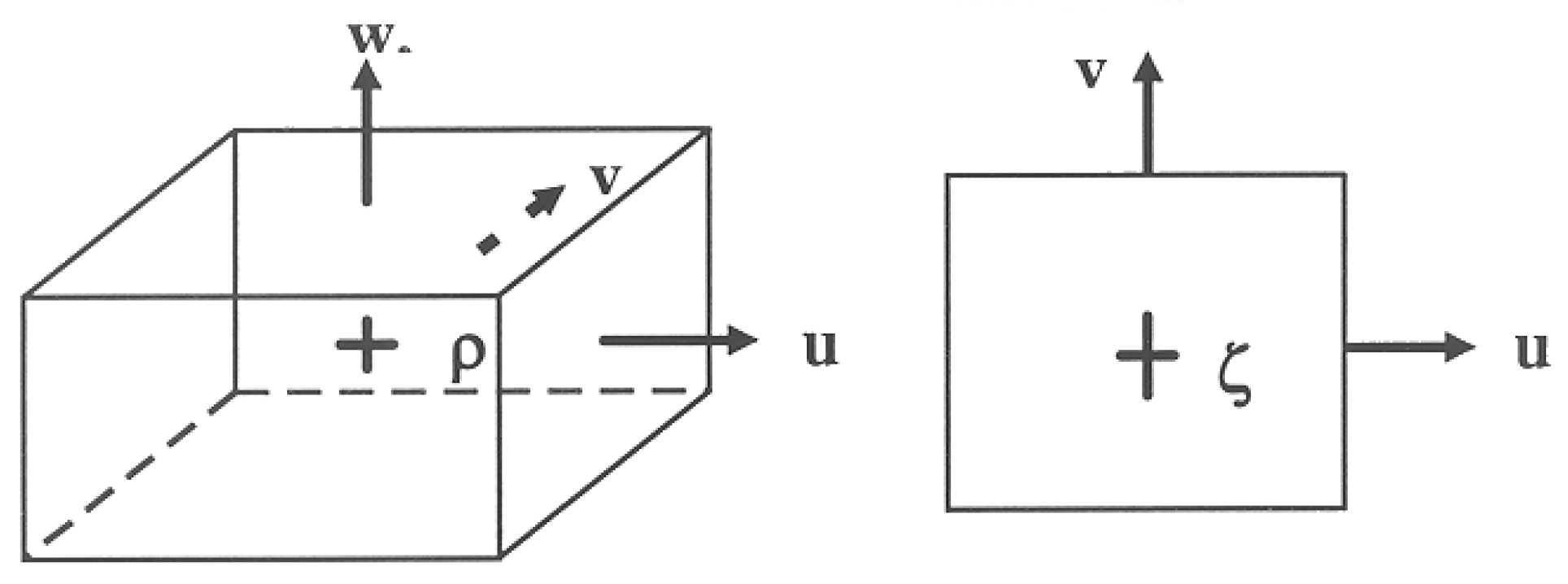
4.2. Discretization and Grid Staggering
The primitive variables water level ζ and velocity components u, v and w describe the flow. To discretize the shallow water equations, we applied a staggered grid finite-difference approach; see Figure 1. This particular arrangement of the variables is called the Arakawa C-grid. The water level points were defined in the centre of a (continuity) cell. The velocity components were perpendicular to the grid cell faces where they were situated.
Staggered grids have several advantages. A smaller number of discrete state variables is required in comparison with discretizations on non-staggered grids to obtain the same accuracy. Boundary conditions can be implemented in a comparatively simple way. Staggered grids for shallow water solvers also prevent spatial oscillations in the water levels and improve robustness [30]. This Arakawa C-grid approach is very common and is used in about 85% of the shallow water models on structured grids [31].
4.3. Discretization of the Advection Terms
The discretizations with i,j refer to the cell numbers in x- and y-directions, respectively, along with their Ui,j and Vi,j velocities in both directions in the grid cell (i,j):
The discretizations in Equations (16) and (17) are both second-order schemes, which yield a third-order reduced phase error scheme for the whole time step [29]. In this way, the numerical dissipation is small but still enough to damp unphysical oscillations that occur from, for example, the open boundaries. This approach is also used in Delft3D-FLOW [32].
4.4. Drying and Flooding
Wetting and drying are important features in shallow water modelling. The water depth H at the u- or v-velocity points should always be positive to guarantee a realistic discharge across a cell face. The same holds for the water depth at cell centres at which the water elevation is computed. Therefore, for both the explicit methods in Equations (11) and (13) and the semi-implicit method in Equation (14), a variable time step approach was applied so that positive water depths are always computed. If the water depth at either water level points or velocity points drops below a certain threshold value, then these computational cells or cell faces are set to be temporarily dry.
4.5. Non-Uniform Grids
The implementation of the numerical methods in Equations (11), (13) and (14) allowed for the use of non-uniform grids. In numerous shallow water applications on a GPU, rectilinear grids are applied. For many applications, for example, for high-resolution inundation studies, this is most likely the best approach. However, in our test cases, we wanted to make a comparison with existing real-life models as well, which were based on curvilinear grids.
The introduction in the 1980s of orthogonal curvilinear and spherical grid transformations for finite difference grids made it possible to design finite difference grids in a flexible way for the optimal representation of specific geometric features while keeping the computational effort acceptable. In [33], it was shown that a unified approach for accurate finite difference modelling exists that largely circumvents the problems that arise due to staircase-type boundary representations while maintaining the computational efficiency of spherical grids and curvilinear grids. A unified formulation for the three-dimensional shallow water equations was developed that covers all orthogonal horizontal grid types of practical interest, which involves orthogonal coordinates on a plane (rectilinear and curvilinear) and orthogonal coordinates on the globe (spherical and spherical curvilinear). Non-uniform grids can lead to much more efficient models compared with uniform rectilinear grids [33]. This is valid for both CPU- and GPU-based systems because the introduction of non-uniform grids hardly requires more computations compared with uniform grids. It does however require more memory and memory bandwidth because extra arrays have to be stored and loaded from memory.
4.6. Solving the Pentadiagonal System
For the semi-implicit time integration method in Equation (14), a pentadiagonal system has to be solved. This system is symmetric and positive definite, which enables the use of the conjugate gradient method. The CG method is the most prominent iterative method for solving sparse systems of linear equations with symmetric positive definite (SPD) coefficient matrices and this method is parallelizable.
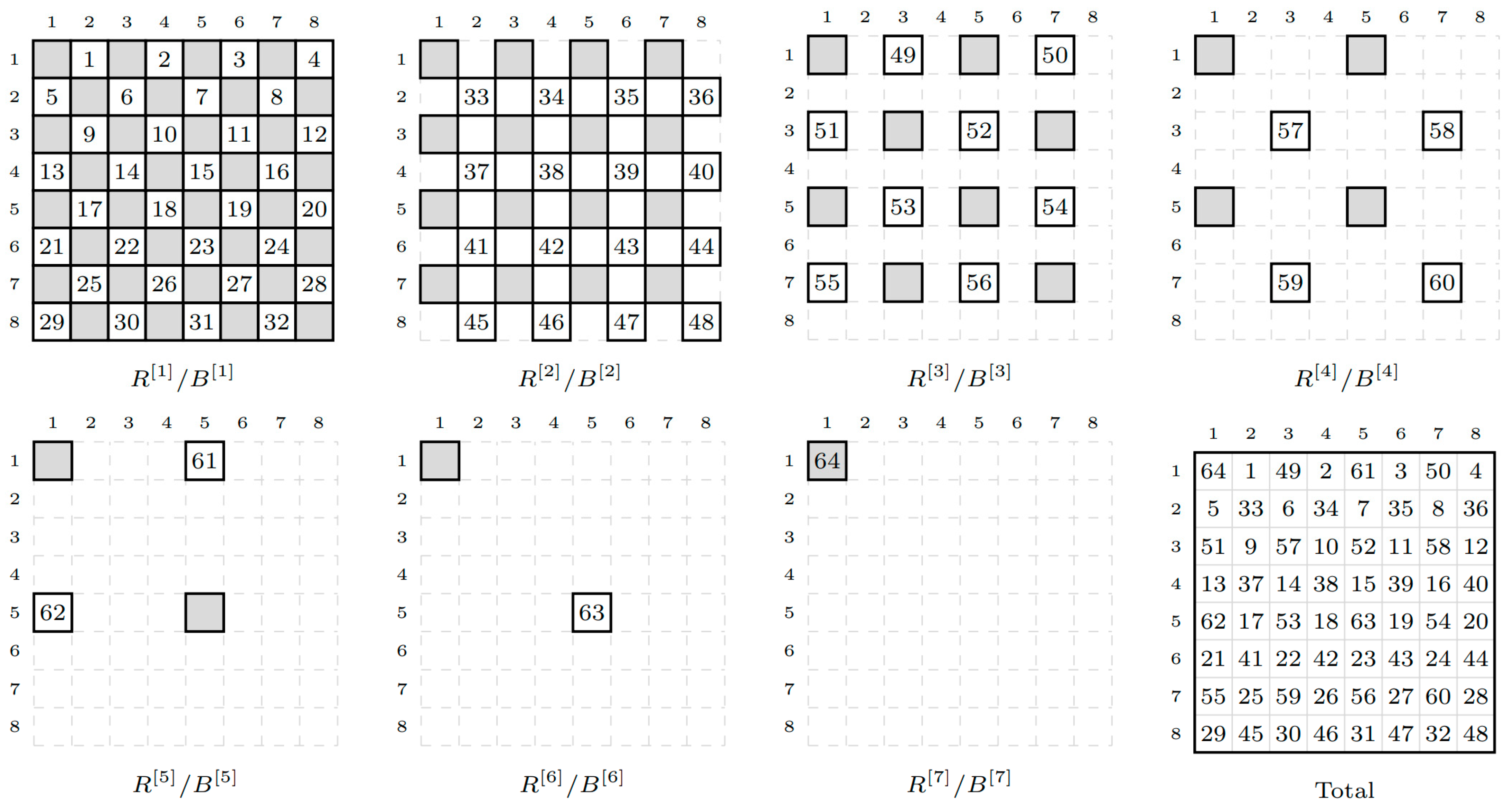
The performance of an iterative method highly depends on the quality of the preconditioner. This is also problem dependent, which makes preconditioning methods a promising and active field of research. In [34], a lot of different preconditioning methods were tested on a GPU. The repeated red black (RRB) method developed in [35] appeared to be the most efficient. This repeated red black method is a multicolouring algorithm that identifies groups of nodes that can be factorized in parallel. The main idea is that the Cholesky factorization method used to construct the preconditioner only requires information from neighbouring points. A 2-level colouring would then lead to a checkerboard pattern and both sets of points can be factorized in parallel. The RRB proceeds to recursively apply this principle until the number of nodes left is so small that parallel factorization no longer provides a speedup. This is illustrated in Figure 2 for seven RRB renumbering levels on an 8-by-8 grid. The RRB solver scales nearly as well as Multigrid and can be parallelized very efficiently on GPUs. On a GPU with a peak bandwidth of 193 GB/s, the performance of the separate routines of the CUDA RRB solver varied between 148 and 188 GB/s for a 2048-by-2048 domain.
In [18], it was demonstrated that the RRB solver allows for the efficient parallelization of both the construction and the application of the preconditioner. Speedup factors of more than 30 were achieved compared with a sequential implementation on the CPU. We used the GPU implementation of the RRB solver in [18,35] as a starting point and optimized the data transfer between the CPU and GPU kernel in order to successfully apply this method for time-dependent simulations.
5. GPU Computing
5.1. GPU Architecture
A graphics processing unit, or a GPU, was primarily developed for efficiently generating computer graphics for display devices. It appeared that with the right programming, they could also be used for numerical computations. Then, the field of general-purpose GPU programming (GPGPU) was born. Modern GPUs can be extremely efficient for parallel computing and the use of GPU programming has vastly increased in recent years.
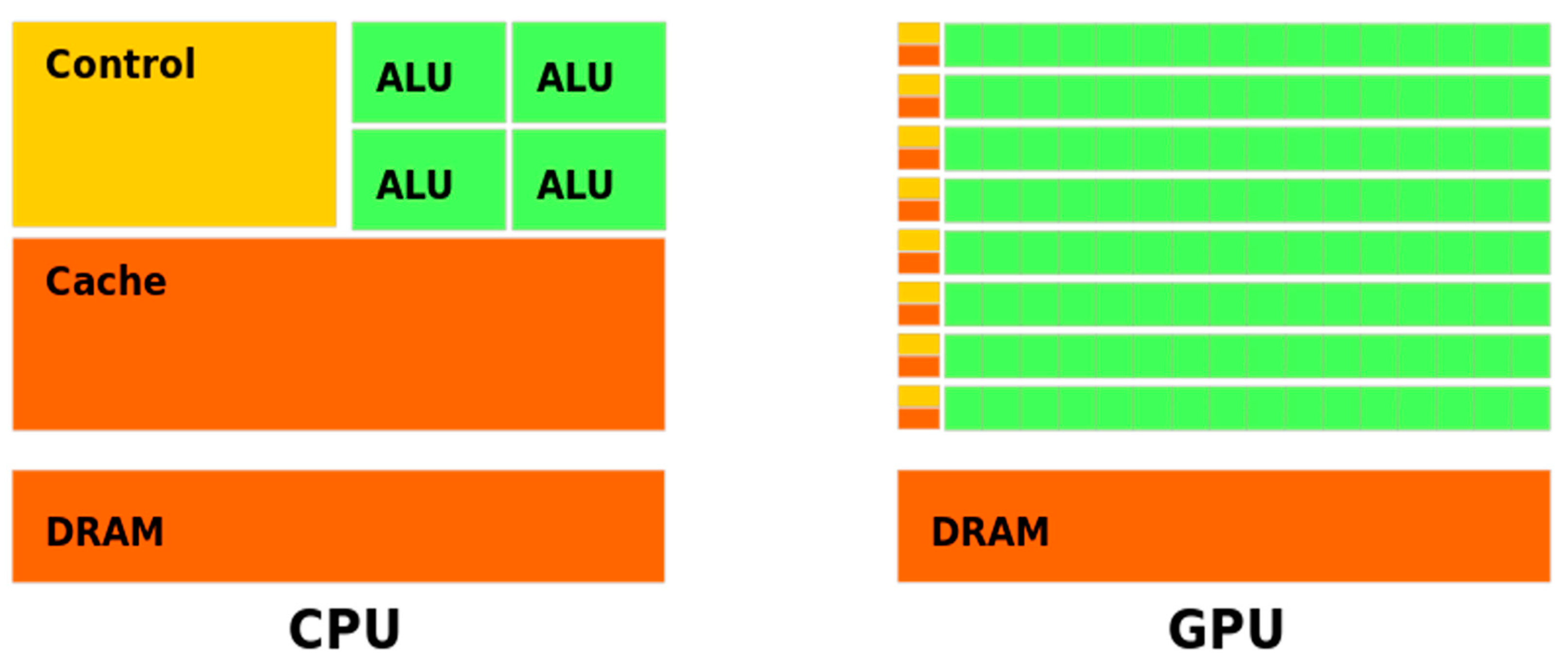
A central processing unit, or a CPU, often only has a limited number of arithmetic units, or “cores”, available, and to ensure maximum efficiency, they use a lot of cache and control circuitry to seamlessly switch between complex tasks. The idea of a GPU is that if a workload is uniform, e.g., a lot of arithmetic units need to perform the same operation just on different data, then the ratio of arithmetic logic units to the cache and control can be vastly increased, see Figure 3.
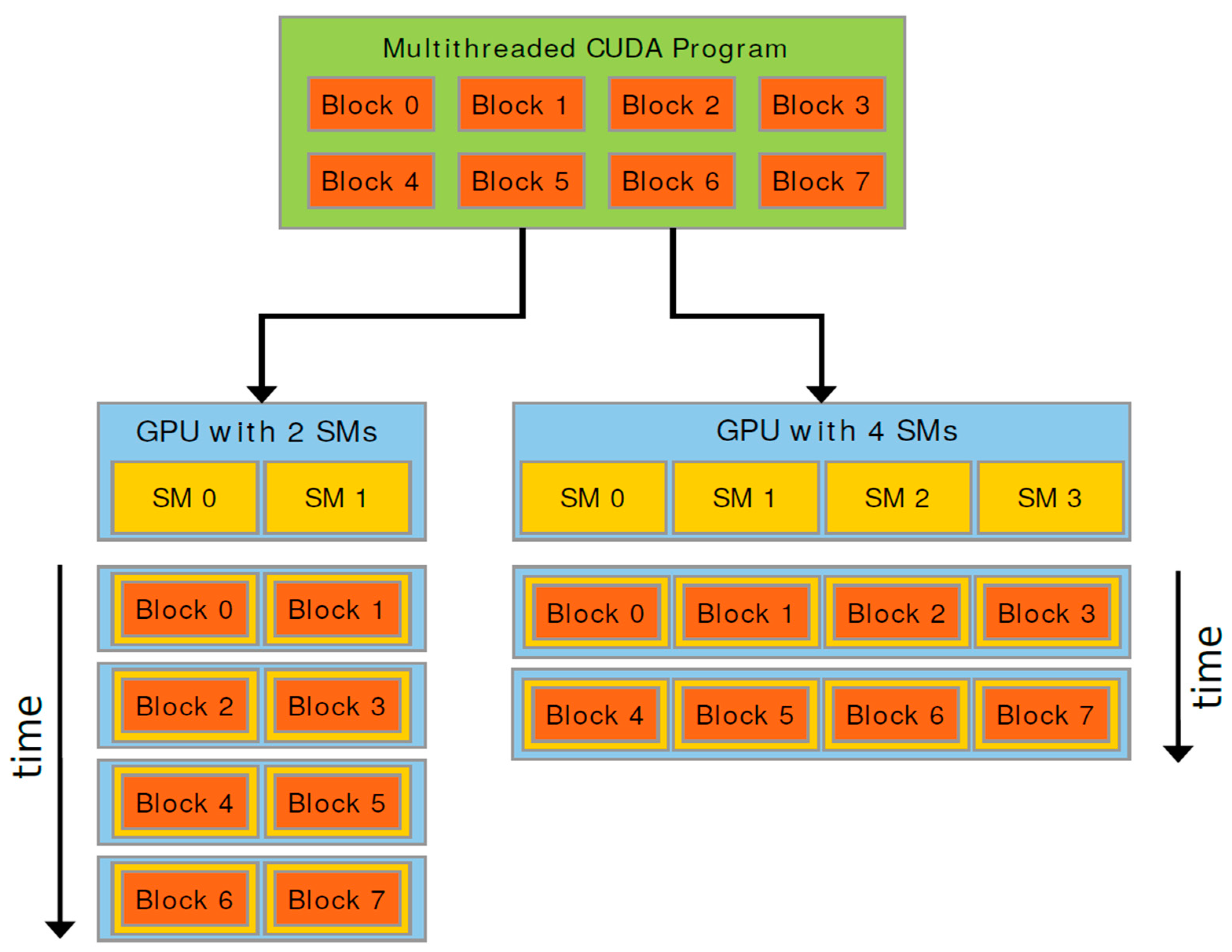
In practice, the GPU has 32 cores for performing the same operation, which is also called a “warp”. Computations sent to the GPU are divided into thread “blocks” that contain an integer number of warps, see Figure 4. A common size is 32 × 32, or 1024 threads per block. These blocks are then asynchronously executed by so-called streaming multiprocessors, each of which can execute a variable number of warps concurrently.
One of the challenges of GPU programming is that only threads within a block can communicate between themselves. If values that reside in a different block are necessary, a completely new workload must be initialized, which can be quite costly.
5.2. Code Implementation
For the efficient use of a GPU, it is necessary that all threads in a warp perform the same operation. For this purpose, thread expression homogeneity was achieved in our code by introducing so-called control Booleans, which were multiplied with parts of the difference equation to dynamically modify it depending on whether the neighbouring velocity points had defined values. This approach is similar to that used in Delft3D [36]. The control Boolean for the x-velocity was called KFU, which is an integer number, with 1 for wet velocity points and 0 for dry or temporarily dry velocity points, as explained in Section 4.4 on drying and flooding. For example, if a computational cell is temporarily dry because of a water depth that is smaller than the threshold depth for drying, then all four cell faces have a Boolean value of 0. The central difference equation for the velocity advection then becomes
Similarly, for the cross-advection term we use for :
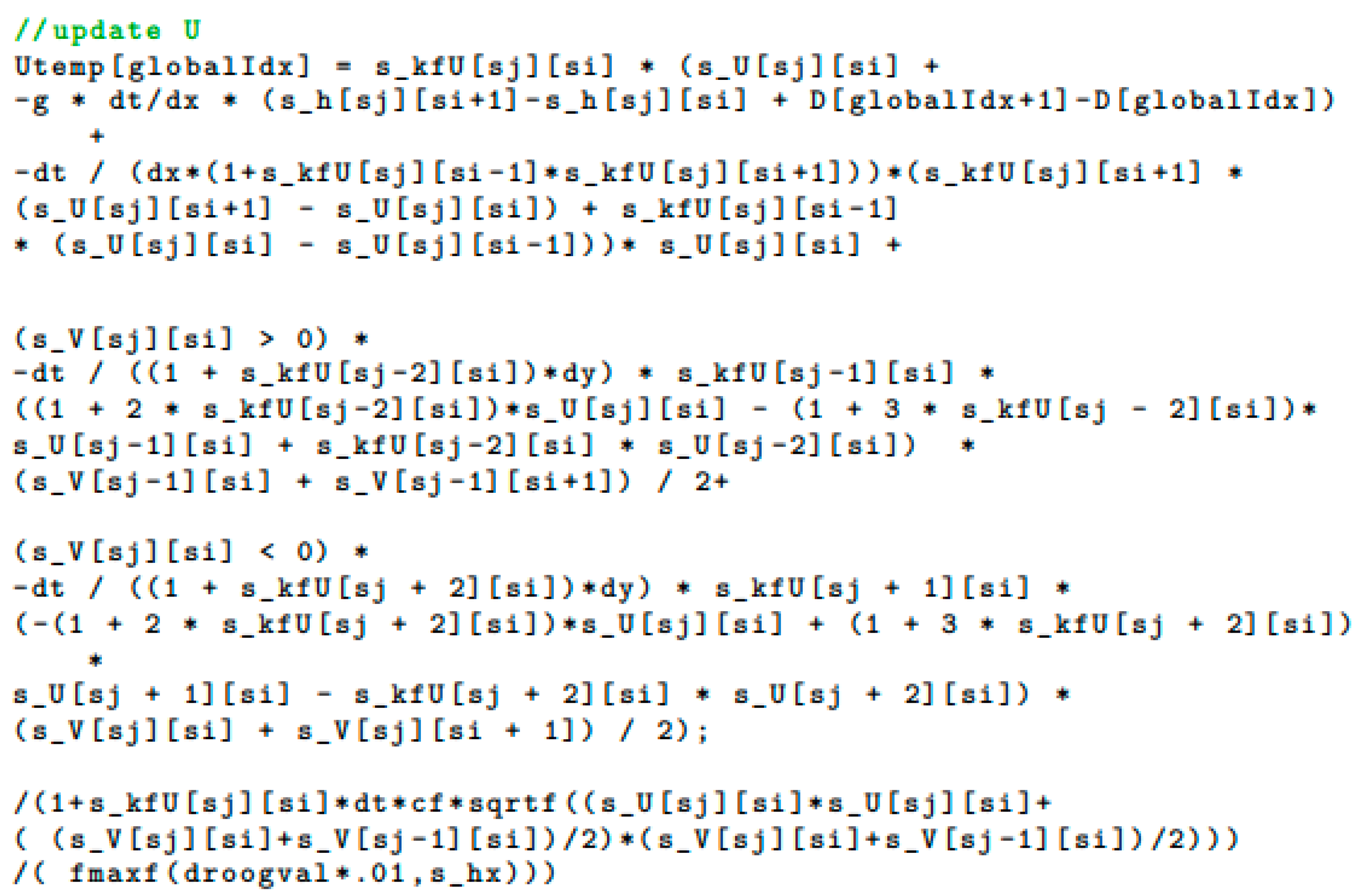
where is the average of the four surrounding V-velocity points at a U-velocity point. In the Appendix A, the CUDA code for the computation of the U-velocity is shown.
6. Model Results
Test cases with increasing complexity were investigated. The first two were schematic test cases, while the third one was a real-life application for the Meuse river in the Netherlands. The simulations were carried out on a machine with both a CPU and a GPU. It consisted of a 6-core CPU (12 threads Intel i7 8086k) together with an NVIDIA RTX 2080 Ti for GPU computing. The Intel i7 8086k operated at 5 GHz with 32 GB of DDR4 DRAM operating at 3200 MHz. The RTX 2080 Ti had 68 streaming multiprocessors, with a total of 4235 CUDA cores operating at 2.16 GHz. It could handle up to 1024 threads per block, with 1024 threads per streaming multiprocessor and 64 registers per thread. It had 11 GB of DDR6 VRAM with a 352-bit memory bus with a maximum bandwidth of 616 GB/s. For the Meuse river test case, the computation times were compared with those found using Delft3D-FLOW, WAQUA and D-Flow Flexible Mesh. These simulations were carried out on a multi-node CPU in which each node consisted of four Intel Xeon 3.60 GHz cores.
6.1. Test Case 1: Simulation of a Water Droplet
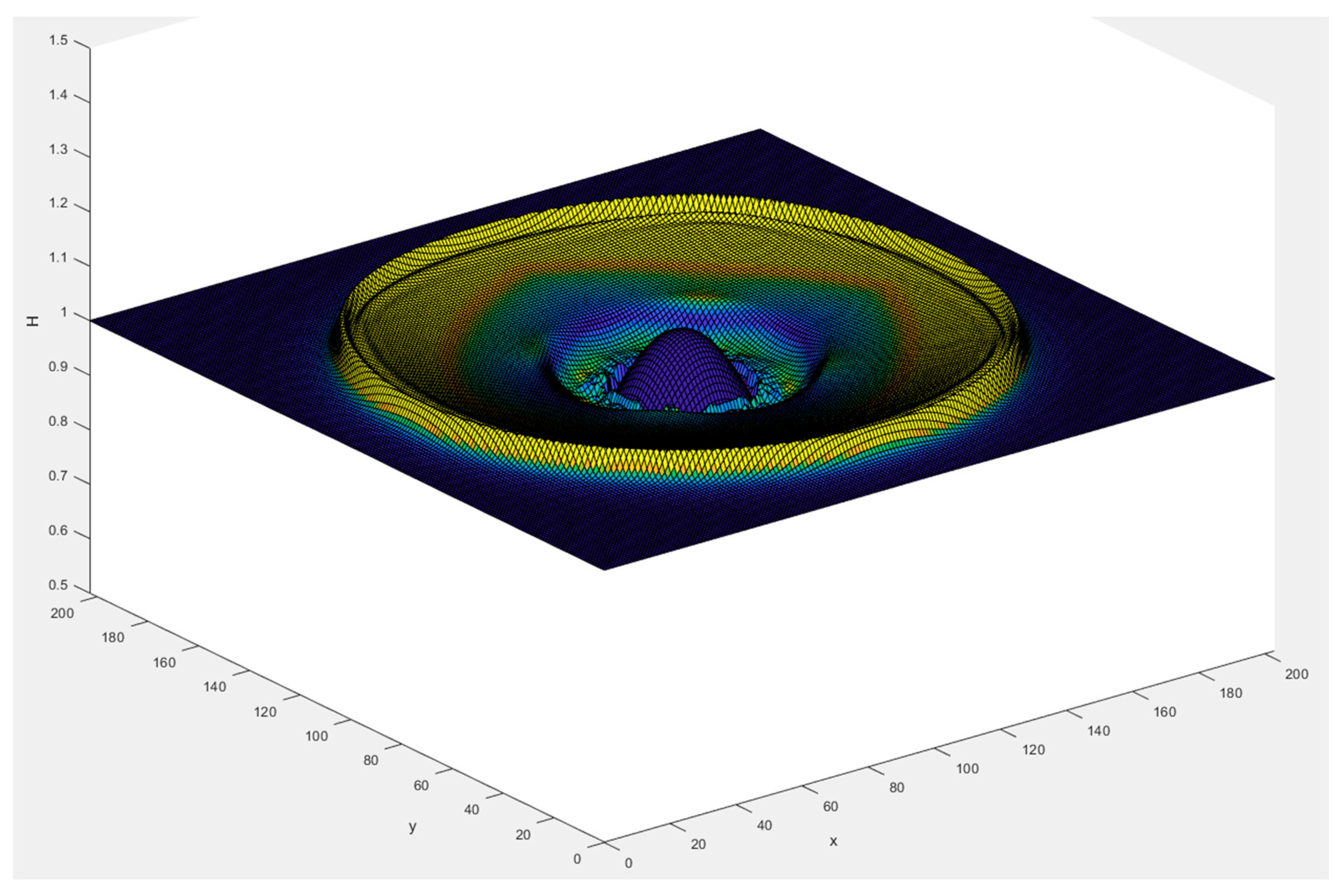
This first test case consisted of a square grid with closed boundaries and initially a Gaussian perturbation of the water level of maximally 1 m to simulate a water droplet, see Figure 5. This produced a ring-shaped outgoing wave that reflected off the boundaries. This test case checked the symmetry of the numerical solution in both the x- and y-directions and also the conservation of mass.
The mesh size was 1 m for all model dimensions, with N being the number of grid cells in both the x- and y-directions. Thus, the larger the value of N, the larger the model domain.
In Table 1, the computation times (in seconds) are listed for both a GPU and a CPU. “Expl-H” refers to the Hansen-type method in Equation (13), “Expl-S” to the Sielecki-type method in Equation (11) and “Semi-impl” to the semi-implicit method in Equation (14). On the CPU, only the “Expl-H” method was used, which was the fastest method on the GPU. We remark that on a CPU, both “Expl-H” and “Expl-S” performed similarly. When doubling the value of N, an increase in the computation time of a factor of four was expected because the number of time steps was constant. For the larger values of N, this behaviour can be seen. For N = 6148, with about 37 million grid cells, the two explicit methods were about 250 times faster on the GPU than a single thread CPU. On the CPU with 12 cores, compared with the results on the GPU, the simulations were about 50 times faster for the fastest explicit method. The semi-implicit method was about 14 times slower compared with the two explicit methods on the GPU. The explicit Hansen scheme was about 20% faster compared with the explicit Sielecki scheme because it required one fewer synchronization on a GPU.
6.2. Test Case 2: Schematized Salt Marsh
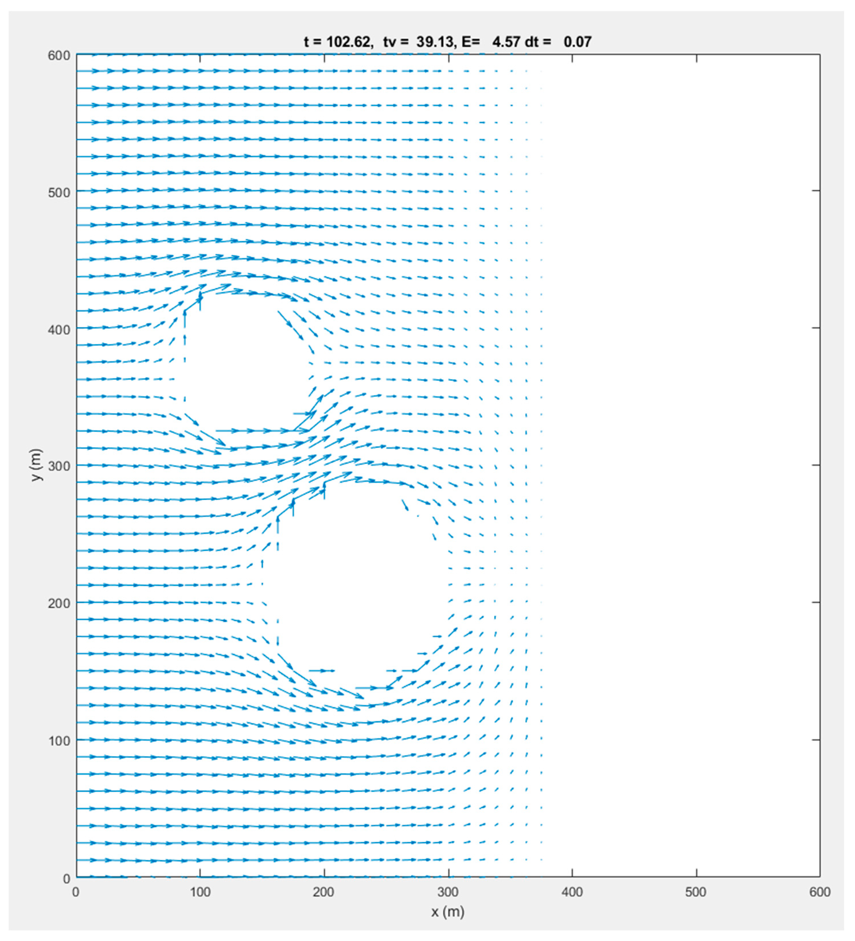
The second test case was taken from [37], which is about salt marsh modelling on a GPU. This test case consisted of a square domain with a width and length of 600 m. The bathymetry varied from 0 m at the left boundary and +4.5 m at the right boundary. At 250 m from the left open boundary, the bathymetry increased linearly from 0 to 4.5 m. A tidal water level was imposed on the left boundary, which was modelled as a sinusoidal function that varied between 1 and 5 m, with a period of 12 h and an initial water level of 3 m. Figure 6 illustrates the water levels at the time for which a water level of 3 m was prescribed at the open boundary. Then, the shallow area with a bathymetry of +4.5 m had become completely dry. We slightly adapted this test case by adding two islands so that the flow became two-dimensional. This is illustrated in Figure 7. The highest currents occurred between these two islands.
In Table 2, the computation times and time step are shown for a simulation period of one day. The average time step is listed because the implemented methods used a dynamic time step, which depended on the currents and the water levels; see the time step conditions in Equations (12) and (15). The number of grid points in the x- and y-directions was equal to N. When doubling N, one expects an eight-fold increase in the computation time because the time step is also halved; see Equation (12). In Table 2, when going from N = 384 to N = 1056, one expects an increase in computation time of about twenty, which was indeed the case. This means that for the larger models, the GPU could use its full speed. This was also observed when compared with the Delft3D-FLOW computation time. For the smaller model of about ten thousand grid cells, the GPU was ten times faster, while for the largest model of about one million grid cells, this was a factor of 100. We remark that the Delft3D-FLOW simulation was carried out on a single core. As expected, the two Delft3D-FLOW simulations had a ratio in computation time of about 1000 because the difference in grid cells was a factor of 10. This semi-implicit method was about twelve times slower compared with the explicit Hansen method for N = 1056. Due to the shallowness of this application, the time step for the semi-implicit method was only 50% larger than for the explicit methods. For deeper applications, this ratio will be much larger, as shown for the next test case. The semi-implicit method (on a GPU) was about ten times faster for N = 1056 compared with Delft3D-FLOW (on a CPU). We remark that the GPU and CPU (Delft3D) simulations were carried out on different hardware platforms. Therefore, the ratios in computation time should be interpreted carefully.
6.3. Test Case 3: River Meuse
6.3.1. Model Description
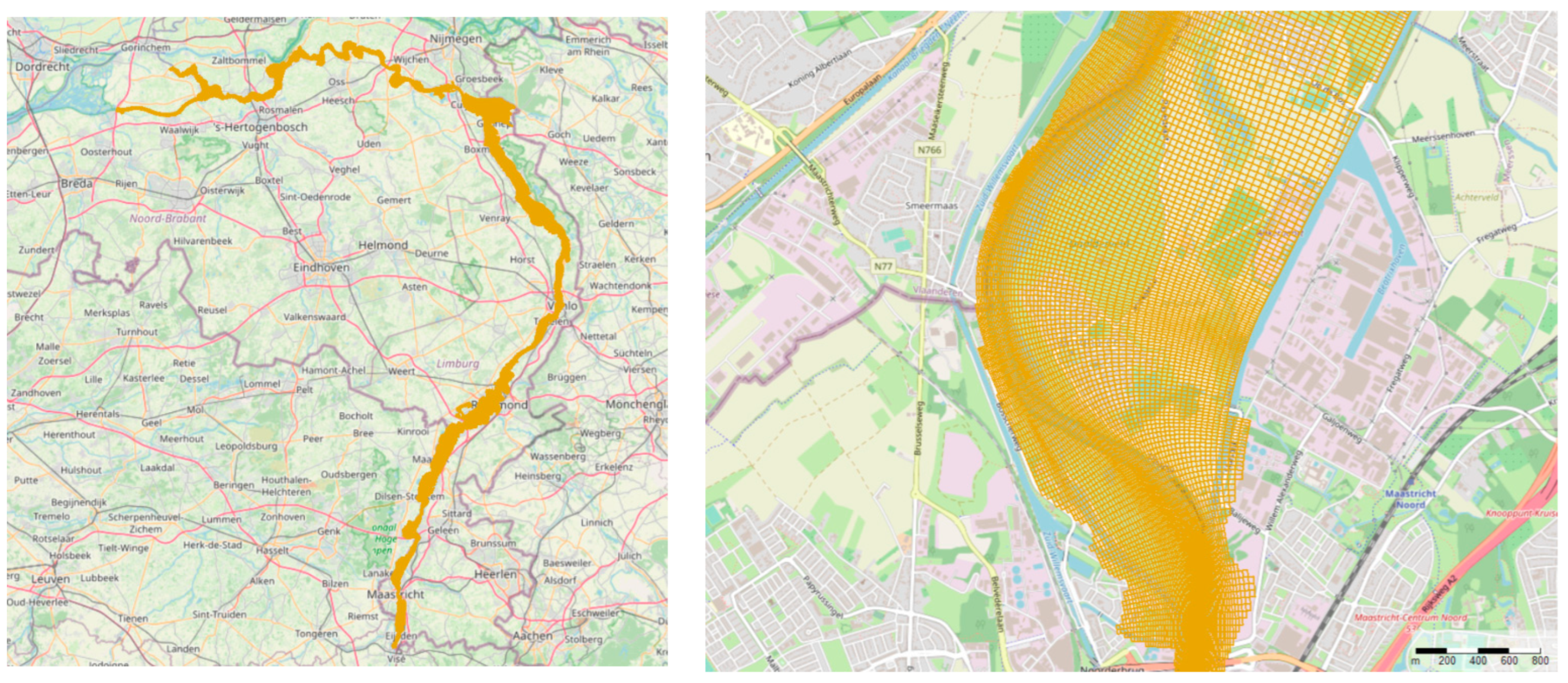
This Meuse model is an operational model in the Netherlands developed by Rijkswaterstaat, which is responsible for the management of water, subsurface, environment and infrastructure in the Netherlands. The Meuse river is the second-largest river in the Netherlands, and the Meuse model is correspondingly an important model that is used for operational water management. The Meuse model was chosen as a test case to show that the newly developed GPU method is applicable to real operational models. The Meuse model area starts upstream at Eijsden, which is close to the Dutch–Belgian border, and the downstream boundary is near Keijzersveer; see Figure 8. The grid is based on a curvilinear grid with about 500,000 grid cells and with mesh sizes varying from 20 to 40 m. The model dimension was about 300-by-3000 grid cells, with about 50% active grid cells and 50% inactive cells (i.e., land points). Note that this is a relatively small test case by GPU standards.
The Meuse is a rain-fed river, which causes large and quick fluctuations in the river discharge. We simulated a peak discharge with a return period of 1250 years, which is the so-called T1250 scenario. This steady-state scenario involves a discharge inflow of 4000 m3/s at the southern inflow boundary and a water level of 3 m at the downstream outflow boundary. At the upstream boundary, the water levels are around +50 m. Thus, the Meuse is a relatively steep river. In combination with the large river inflow of 4000 m3/s, currents up to about 5 m/s can occur. The drying flooding threshold was set to 5 cm.
The Rijkswaterstaat model was simplified. It contains advanced options for hydraulic structures and vegetation, as well as for dykes and groynes; the latter empirical concepts are applied at, for example, the Tabellenboek and Villemonte [38]. The GPU code developed for this study does not contain these advanced options. Therefore, only the model grid and the bathymetry of the Rijkswaterstaat model were used. The water levels in this part of the river Meuse are steered by moveable flood barriers. In the subsection of the Meuse that we simulated, seven barriers exist (Borgharen, Linne, Roermond, Belfeld, Sombeek, Grave and Lith). However, in the case of high water, these barriers are fully open and have a very limited impact on the water levels. Therefore, for the T1250 scenario, it was justified to simplify the Meuse model by neglecting the hydraulic structures for the moveable barriers.
We not only simulated this Meuse model with the GPU methods described in this study but also with Delft3D-FLOW, WAQUA and D-Flow Flexible Mesh, which are Dutch software systems for hydrodynamic modelling on CPU-based systems. The first two systems are based on structured grids and the latter is based on unstructured grids. Nevertheless, D-Flow Flexible Mesh is interesting for this comparison because its numerical approach is close to our semi-implicit method in Equation (14). For a detailed description of the discretizations of Delft3D-FLOW, WAQUA and D-Flow Flexible Mesh, we refer to [28], in which the main characteristics are described, or to the user manuals in [36], [38] and [39], respectively.
6.3.2. Model Results
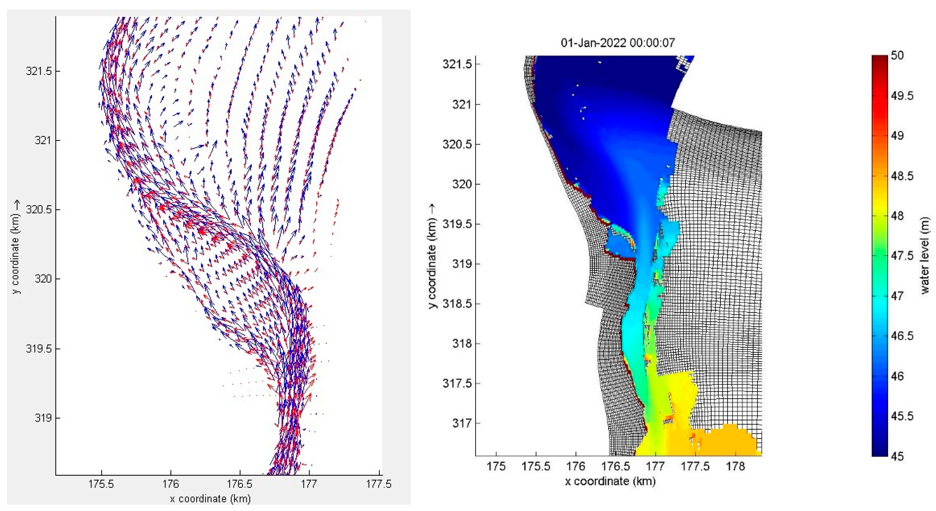
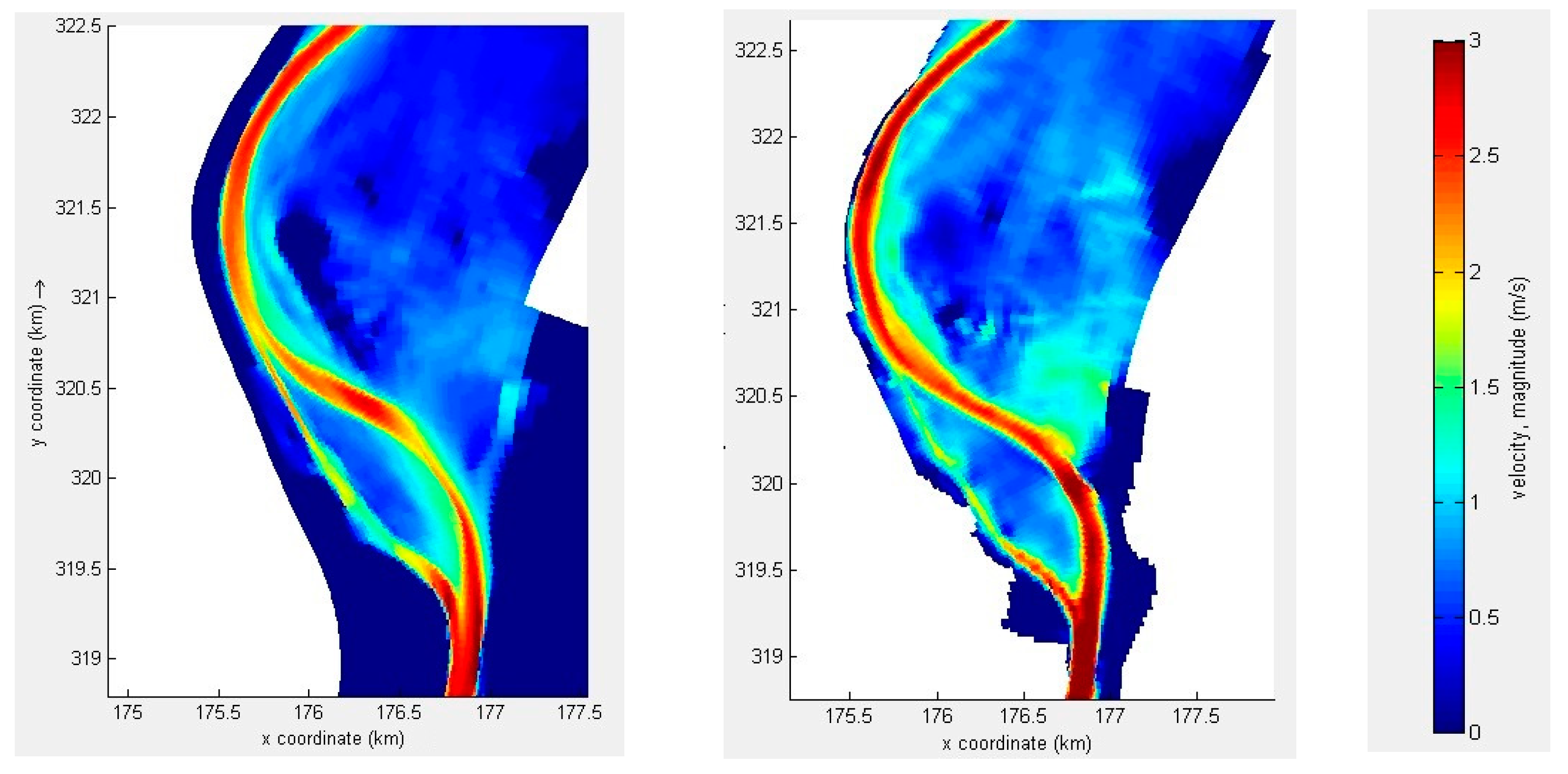
The model results of all codes were in good agreement with each other. In Figure 9 and Figure 10, the currents are illustrated for one of the meandering bends of the Meuse river. It can be seen that the highest currents occurred in the main channel, with much lower currents at the flood plains. In the right panel of Figure 9, it can be seen that part of the model grid was still without any water. These areas, for example, represent cities or villages, which are protected by so-called winter dykes so that these areas never become wet. We remark that the numerical methods in Delft3D-FLOW, WAQUA, D-Flow Flexible Mesh and the numerical methods presented in this paper do not use the same numerical schemes and approaches. Since no analytical solution exists, the model results can only be compared globally. A thorough mathematical analysis of the model results did not fit into the scope of this study. Therefore, in Figure 9 and Figure 10, differences can be observed, but we deem the level of agreement in the model results satisfactory.
In Table 3, the average time steps and the computation times are listed for several software codes. WAQUA and Delft3D-FLOW used a fixed time step, for which the time step was based on accuracy reasons. For the Meuse model, we applied a fixed time step of 7.5 s. The other three methods applied a variable time step. For the GPU methods used in this study, the stability criteria for the time step are in Equations (12) and (15). D-Flow Flexible Mesh used an average time step of 2.3 s, which was more or less comparable to “Semi-impl”, referring to the semi-implicit scheme in Equation (14), for which the average time step was 1.9 s. The explicit methods “Expl-H” and “Expl-S”, referring to the Hansen-type scheme in Equation (13) and the Sielecki-type scheme in Equation (11), respectively, applied a much smaller average time step of 0.2 s because of the explicit time integration method for advection in combination with the high currents of maximally approximately 5 m/s.
With respect to the computation times, the explicit methods “Expl-H” and “Expl-S” were the fastest, with “Expl-H” being the most efficient one because it required one synchronization, or kernel launch, less compared with “Expl-S”. For “Expl-S”, a global thread synchronization was necessary for each quantity, which required three synchronizations per time step, while “Expl-H” only required two. Two instead of three thread synchronizations per time step reduced the computation time by about 15–20%. The two explicit methods on the GPU were about 25 times faster than WAQUA, 50 times faster than Delft3D-FLOW and 75 times faster than D-Flow Flexible Mesh.
The “Semi-impl” method required about 330 s, which was about two times slower than the “Expl-H” method and ten times faster than WAQUA, which was the fastest CPU code. It is known that WAQUA is highly optimized for sequential and parallel simulations for 2D modelling [28]. Therefore, it is plausible that Delft3D-FLOW was about two times slower for this application. Due to the explicit time integration for advection, D-Flow Flexible Mesh required a smaller time step compared with WAQUA and Delft3D-FLOW. Consequently, the computation time was also somewhat larger.
In the variable time step approach, we applied a MAX-function in our code to determine the maximum value for , in which was determined for each computation cell i using stability condition (12) for the two explicit methods and using stability condition (15) for the semi-explicit method. The computation of this MAX-function appeared to be very costly because synchronization was required over all computation cells. As a test, we applied a fixed time steps of 0.2 s for the two explicit methods. Then, the computation times were respectively 69 s and 93 s instead of 132 s and 164 s, which is almost half the computation time in Table 3. This illustrates that the computation of the time step can be further optimized.
We remark that in practice, simulations with WAQUA, Delft3D-FLOW and D-Flow Flexible Mesh are often carried out in parallel mode via the distributed memory approach by using MPI for data transfer between the notes. This significantly reduces computation times, which is illustrated in Table 3 by using 4 or 16 cores. For the GPU-based method, we have not developed a multi-node implementation yet, which is possibly one of the future activities for further improvement.
In summary, the ratio in computation time between the GPU- and CPU-based methods should be interpreted carefully. For example, the GPU code runs in single precision, while the other three systems run in double precision. The hardware is also rather different. Nevertheless, a computation time of about two minutes for the explicit method on an “off-the-shelf” GPU system is impressive. With a multi-node CPU-based system, this will probably never be reached. For a large number of cores, the overhead in communication between the nodes will become larger than the reduction in time for the computations, thus leading to larger computation times. Moreover, this Meuse test case only had about half a million grid points, which is relatively small for a GPU application. For applications with much more grid points, the GPU is expected to perform even better compared with a CPU.
7. Discussion on GPU versus CPU Computing
The performance results of Section 6 clearly show the huge potential of GPU computing for the shallow water equations. In this section, we compare these results with other publications on GPU- versus CPU-based methods for the 2D depth-averaged SWEs on structured grids.
7.1. Ratio of GPU versus CPU Timings for Other SWE Codes
In [9], a GPU implementation was developed for an explicit time integration method. This so-called Iber+ system appeared to be 100 times faster on a GPU than on a CPU. In that study, it was also concluded that “for an extreme flash flood that took place in the Spanish Pyrenees in October 2012 the GPU-based system Iber+ was able to simulate 24 h of physical time in less than 10 min using a numerical mesh of almost half a million elements. The same case run with the standard version needs more than 15 h of CPU time. This is more or less comparable to our river Meuse application of about half a million grid points that requires a few minutes of computation time for a 1-day simulation.
In [39], the Sielecki-type scheme of Equation (11) was implemented on a GPU and appeared to be a factor of 200 faster than the same method on a CPU. In [15], the MIKE21 method for 2D modelling was implemented on a GPU and appeared to be about 50 times faster for double-precision and about 150 times faster for single-precision compared with the CPU performance. According to [40], on a single processor, the GPU version of MIKE21 can be a factor of 100 or more faster compared with the CPU version. Switching from one to four GPU cards yields another factor of up to three, leading to a total speedup in the order of 300 for the GPU compared to the CPU.
In summary, in several studies on 2D modelling for the SWEs, it was demonstrated that on a GPU, significantly lower computation times can be achieved in comparison to CPU-based systems. Our study is another one that shows that GPU-based computing for the SWEs can lead to computation times that are an order of magnitude smaller compared with computation times on a CPU-based system. Next to the significant reduction in computation time, it also opens the possibility to go to much higher resolution modelling, with mesh sizes in the order of a few meters, while for CPU-based system operational models, the mesh sizes in general remain in the order of tens of meters (10 to 25 m) for large-scale applications.
7.2. Advantages of GPU Computing over CPU Computing
GPU computing enables modelling on a higher resolution; for example with meshes in the order of a few metres. This also offers advantages with respect to the modelling approach:
- Fewer numerical approximations: For example, for groynes in Dutch river models, a complex empirical approach is applied in current SWE models [38]. This yields accurate water levels, but currents around groynes are inaccurate. It should be noted that this empirical approach is not meant for simulating accurate currents. With GPU computing, a grid resolution of a few metres becomes possible so that groynes can now be schematized in the bathymetry. Then, this empirical approach is no longer required. In this way, not only water levels but also currents can be computed accurately. The latter is also relevant for morphodynamic scenarios, in which the time evolution of the bathymetry is simulated.
- Easier preprocessing of models: The set-up of operational SWE models in the Netherlands is being done automatically. The coarser the resolution, the more complex the approach. For example:
- Vegetation: For each computation cell, the bed roughness is generated. For example, a grid cell might consist of 30% buildings, 20% hedges and 50% grass, each of which has a different roughness. Via a complex algorithm, this is converted into a roughness coefficient per grid cell. On a high-resolution GPU model, each grid cell will have only one vegetation type.
- Height model: When using 25 m-resolution small levees, heightened roads and traffic bumps may be removed from the height model due to averaging the height values. To fix this, a user can sometimes increase the height artificially, but this requires additional work and can result in mistakes. A high-resolution GPU model does not have this problem because geographical objects, such as roads, speed bumps and levees, show up in the high-resolution grid of approximately 1 m.
An illustration of high-resolution SWE modelling on a GPU can be found on the Tygron Geodesign Platform [41]. This is based on an SWE model that is second-order well-balanced positivity preserving and is based on the schema developed by Kurganov and Petrova [42]. The model schema is explicit and was adapted to work in a multi-GPU configuration on the latest 64-bit data centre GPU nodes. This scheme is further extended with the shoreline reconstruction method by Bollerman [43] which ensures better numerical stability at the wetting and drying fronts of a flood wave. To prevent negative water levels in drying fronts, a draining time step is used. The SWE scheme is integrated into a larger GPU model that also simulates hydraulic structures (weirs, culverts, inlets) and dam breaches based on a 2D grid with conservation of momentum. The model is optimized to run on multiple GPUs using the CUDA architecture but can also run in a CPU Java environment for extensive testing and comparing of CPU and GPU results. This allows the model to run up to 10 billion grid cells in a multi-GPU configuration connected via NVLINK for an artificial flooding event in the Netherlands [44].
8. Conclusions
In this study, explicit and semi-implicit time integration methods were developed for the depth-averaged (2D) shallow water equations on a structured grid for GPUs. The methods are suitable for both rectangular, curvilinear and spherical grids. Both methods are of the finite-difference type and allow for drying and flooding. For the discretization of the advection terms, the combination of second-order central discretizations and second-order upwind scheme leads to a fourth-order dissipation, which suppresses any unphysical oscillations. The semi-implicit time integration method is based on an operator splitting technique, which is a novel approach for the shallow water equations on GPUs. It requires the solution of a Poisson-type equation, for which a repeated red black (RRB) solver is used. This solver has a very good convergence behavior and can also be implemented efficiently on GPUs. The RRB solver scales nearly as well as Multigrid and the throughput number in memory bandwidth in GB/s is about 75% of the peak performance on a modern GPU.
Two schematic test cases were examined with up to about 150 million grid points. Furthermore, a real-life model application for the river Meuse in the Netherlands was tested, which consisted of about half a million grid points. For these three test cases, the explicit method was faster than the semi-implicit method on a GPU. This was mainly due to the fact that these three test cases were relatively shallow, with depths of up to approximately 20 m. For much deeper applications, such as the Dutch Continental Shelf model with depths up to 5 km, the semi-implicit method will most likely be faster. We conclude that both explicit and semi-implicit time integration methods can run efficiently on a GPU, with realistic use cases for both methods.
For the river Meuse application, the model results and the computation time were compared with the ones for existing hydrodynamic software systems in the Netherlands, namely, Delft3D, Simona and Delft3D Flexible Mesh. A thorough mathematical analysis of the model results did not fit into the scope of this study; however, the results of these four software systems were in sufficient agreement with each other. The ratio in computation time between the GPU and the CPU was in the order of 25 to 75. Our Meuse test case with only about half a million grid points was rather small by GPU standards, and thus, as expected, the speedup for the Meuse model was relatively small.
The findings in this study confirmed what was reported in other GPU papers for the depth-averaged SWEs, namely, that computation on GPUs can be an order of magnitude faster—roughly 50 to 100 times—compared with CPUs. This also allows for high-resolution applications for the SWEs on GPUs. Currently, a resolution of about 25 m is used in operational Dutch SWE models on CPUs. By using GPUs, high-resolution models (5-by-5 m or even 1-by-1 m) can be simulated in a reasonable time, as is shown in a model of the Netherlands including all major rivers.
An implicit time integration method for the advective terms could be a topic of future research. The implicit time integration of advection in Delft3D-FLOW via a Jacobi-type iterative solver might be a GPU-suitable candidate for this. If this is applied to the semi-implicit method in Equation (14), then the time step limitation in Equation (15) disappears, which allows the time step to be chosen based on accuracy requirements. A second topic of future research is an extension to multi-GPUs, which is expected to further improve the performance of large models.
Author Contributions
Conceptualization: F.J.L.B., E.D.G. and C.V.; methodology: F.J.L.B., E.D.G. and C.V.; software: F.J.L.B.; validation: F.J.L.B., E.D.G., M.K. and C.V.; formal analysis: F.J.L.B.; investigation: F.J.L.B.; resources: F.J.L.B., E.D.G. and M.K.; data curation: F.J.L.B.; writing—original draft preparation: E.D.G. (major), F.J.L.B. (minor) and M.K. (minor); writing—review and editing: E.D.G., F.J.L.B., M.K. and C.V.; project administration: C.V.; funding acquisition: E.D.G. and C.V. All authors have read and agreed to the published version of the manuscript.
Funding
This research received no external funding, except in-kind contributions from Deltares, Delft University of Technology and Tygron.
Institutional Review Board Statement
Not applicable.
Informed Consent Statement
Not applicable.
Data Availability Statement
The data presented in this study are available on request from the corresponding author. The data are not publicly available due to significant parts of the data consisting of a proprietary model belonging to Deltares.
Acknowledgments
Most of the work of this study was carried out during the Master‘s thesis of Buwalda [34] at the Delft University of Technology. The Maritime Research Institute Netherlands (MARIN) is thanked for providing the GPU implementation of the RRB solver developed by De Jong [18,35]. The anonymous reviewers are thanked for their valuable remarks and for informing us about other GPU papers, as well as the incompressible Navier–Stokes equations.
Conflicts of Interest
The authors declare no conflict of interest.
Appendix A
For illustration, in Figure A1 the CUDA code is shown for the computation of the U-velocity at the new time level. Despite the fact that a complex numerical scheme is applied, which is described in detail in Section 4, the CUDA code is considered to be relatively easy and readable.
Figure A1.
Illustration of the CUDA code.

Next to the integer values for either a wet or dry status (see, for example, ), the code also contained Booleans (see, for example, ) in order to apply either upwinding or downwinding, which depends on the sign of the V-velocity. In this way, IF statements were circumvented. For the explicit numerical schemes in Equations (11) and (13), the value of grid cell (i,j) at the next timestep can be computed independently of all other grid cells. Such computations are perfectly suited for a GPU because the GPU is a highly parallel processor.
References
- Krüger, J.; Westermann, R. Linear algebra operators for GPU implementation of numerical algorithms. ACM Trans. Graph. 2003, 22, 908–916. [Google Scholar] [CrossRef]
- Du, P.; Weber, R.; Luszczek, P.; Tomov, S.; Peterson, G.; Dongarra, J. From CUDA to OpenCL: Towards a performance-portable solution for multi-platform GPU programming. Parallel Comput. 2012, 38, 391–407. [Google Scholar] [CrossRef] [Green Version]
- Klingbeil, K.; Lemarié, F.; Debreu, L.; Burchard, H. The numerics of hydrostatic structured-grid coastal ocean models: State of the art and future perspectives. Ocean. Model. 2018, 125, 80–105. [Google Scholar] [CrossRef] [Green Version]
- Vreugdenhil, C.B. Numerical methods for shallow-water flow. In Water Science and Technology Library; Kluwer Academic Publishers: Dordrecht, The Netherlands, 1994; ISBN 0-7923-3164-8. [Google Scholar]
- Aureli, F.; Prost, F.; Vacondio, R.; Dazzi, S.; Ferrari, A. A GPU-accelerated shallow-water scheme for surface runoff simulations. Water 2020, 12, 637. [Google Scholar] [CrossRef] [Green Version]
- Brodtkorb, A.; Hagen, T.R.; Roed, L.P. One-Layer Shallow Water Models on the GPU. Norwegian Meteorological Institute Report No. 27/2013. 2013. Available online: https://www.met.no/publikasjoner/met-report/met-report-2013/_/attachment/download/1c8711b6-b6c2-45f6-985d-c48f57b1d921:337ce17f6db07903d6f35919717c1d80c8756cc9/MET-report-27-2013.pdf (accessed on 14 March 2023).
- Dazzi, S.; Vacondio, R.; Dal Palu, A.; Mignosa, P. A local time stepping algorithm for GPU-accelerated 2D shallow water models. Adv. Water Resour. 2018, 111, 274–288. [Google Scholar] [CrossRef]
- Fernández-Pato, J.; García-Navarro, P. An Efficient GPU Implementation of a Coupled Overland-Sewer Hydraulic Model with Pollutant Transport. Hydrology 2021, 8, 146. [Google Scholar] [CrossRef]
- García-Feal, O.; González-Cao, J.; Gómez-Gesteira, M.; Cea, L.; Domínguez, J.M.; Formella, A. An Accelerated Tool for Flood Modelling Based on Iber. Water 2018, 10, 1459. [Google Scholar] [CrossRef] [Green Version]
- Guerrero Fernandez, E.; Castro-Diaz, M.J.; Morales de Luna, T. A Second-Order Well-Balanced Finite Volume Scheme for the Multilayer Shallow Water Model with Variable Density. Mathematics 2020, 8, 848. [Google Scholar] [CrossRef]
- Parma, P.; Meyer, K.; Falconer, R. GPU driven finite difference WENO scheme for real time solution of the shallow water equations. Comput. Fluids 2018, 161, 107–120. [Google Scholar] [CrossRef] [Green Version]
- Smith, L.S.; Liang, Q. Towards a generalised GPU/CPU shallow-flow modelling tool. Comput. Fluids 2013, 88, 334–343. [Google Scholar] [CrossRef]
- Xu, S.; Huang, S.; Oey, L.-Y.; Xu, F.; Fu, H.; Zhang, Y.; Yang, G. POM.gpu-v1.0: A GPU-based Princeton Ocean Model. Geosci. Model Dev. 2015, 8, 2815–2827. [Google Scholar] [CrossRef] [Green Version]
- Zhao, X.D.; Liang, S.-X.; Sun, Z.-C.; Liu, Z. A GPU accelerated finite volume coastal ocean model. Sci. Direct 2017, 29, 679–690. [Google Scholar] [CrossRef]
- Aackermann, P.E.; Dinesen Pedersen, P.J. Development of a GPU-Accelerated MIKE 21 Solver for the Water Wave Dynamics; Technical University of Denmark: Lyngby, Denmark, 2012. [Google Scholar]
- Zhang, Y.; Jia, Y. Parallelized CCHE2D flow model with CUDA Fortran on Graphics Processing Units. Comput. Fluids 2013, 84, 359–368. [Google Scholar] [CrossRef]
- Esfahanian, V.; Baghapour, B.; Torabzadeh, M.; Chizari, H. An efficient GPU implementation of cyclic reduction solver for high-order compressible viscous flow simulations. Comput. Fluids 2014, 92, 160–171. [Google Scholar] [CrossRef]
- De Jong, M.; Van der Ploeg, A.; Ditzel, A.; Vuik, C. Fine-grain parallel rrb-solver for 5-/9-point stencil problems suitable for GPU-type processors. Electron. Trans. Numer. Anal. 2017, 46, 375–393. [Google Scholar]
- Aissa, M.; Verstraete, T.; Vuik, C. Toward a GPU-aware comparison of explicit and implicit CFD simulations on structured meshes. Comput. Math. Appl. 2017, 74, 201–217. [Google Scholar] [CrossRef]
- Ha, S.; Park, J.; You, D. A GPU-accelerated semi-implicit fractional-step method for numerical solutions of incompressible Navier–Stokes equations. J. Comput. Phys. 2018, 352, 246–264. [Google Scholar] [CrossRef]
- Zolfaghari, H.; Obrist, D. A high-throughput hybrid task and data parallel Poisson solver for large-scale simulations of incompressible turbulent flows on distributed GPUs. J. Comput. Phys. 2021, 437, 110329. [Google Scholar] [CrossRef]
- Morales-Hernandez, M.; Kao, S.-C.; Gangrade, S.; Madadi-Kandjani, E. High-performance computing in water resources hydrodynamics. J. Hydroinf. 2020, 22, 1217–1235. [Google Scholar] [CrossRef] [Green Version]
- Hansen, W. Theorie zur Errechnung des wasserstandes und der Strömingen in Randmeeeren nebst Anwendungen. Tellus 1956, 8, 289–300. [Google Scholar] [CrossRef] [Green Version]
- Heaps, N.S. A two-dimensional numerical sea model. Phil. Trans. Roy. Soc. 1969, 265, 93–137. [Google Scholar]
- Sielecki, A. Mathematical Weather Rev; U.S. Department of Agriculture: Washington, DC, USA, 1968; Volume 96, pp. 150–156.
- Backhaus, J.O. A semi-implicit scheme for the shallow water equations for application to shelf sea modelling. Cont. Shelf Res. 1983, 2, 243–255. [Google Scholar] [CrossRef]
- Casulli, V.; Cheng, R.T. Semi-implicit finite difference methods for three-dimensional shallow water flow. Int. J. Numer. Methods Fluids 1992, 15, 629–648. [Google Scholar] [CrossRef]
- De Goede, E.D. A time splitting method for the three-dimensional shallow water equations. Int. J. Numer. Meth. Fluids 1991, 13, 519–534. [Google Scholar] [CrossRef]
- Wilders, P.; Van Stijn, T.L.; Stelling, G.S.; Fokkema, G.A. A fully implicit splitting method for accurate tidal computations. Int. J. Num. Methods Eng. 1988, 26, 2707–2721. [Google Scholar] [CrossRef]
- Stelling, G.S. On the Construction of Computational Methods for Shallow Water Problems. Ph.D. Thesis, Delft University of Technology, Delft, The Netherlands, 1983. [Google Scholar]
- Jones, J.E. Coastal and shelf-sea modelling in the European context. Oceanogr. Mar. Biol. Annu Rev. 2002, 40, 37–141. [Google Scholar]
- Gerritsen, H.; De Goede, E.D.; Platzek, F.W.; Genseberger, M.; Van Kester, J.A.T.H.M.; Uittenbogaard, R.E. Validation Document Delft3D-FLOW, WL|Delft Hydraulics Report X0356/M3470. 2008. Available online: https://www.researchgate.net/publication/301363924_Validation_Document_Delft3D-FLOW_a_software_system_for_3D_flow_simulations (accessed on 12 March 2023).
- Kernkamp, H.W.J.; Petit, H.A.H.; Gerritsen, H.; De Goede, E.D. A unified formulation for the three-dimensional shallow water equations using orthogonal co-ordinates: Theory and application. Ocean. Dyn. 2005, 55, 351–369. [Google Scholar] [CrossRef]
- Buwalda, F. Suitability of Shallow Water Solving Methods for GPU Acceleration. Master’s Thesis, Delft University of Technology, Delft, The Netherlands, 2020. Available online: https://repository.tudelft.nl/islandora/search/author%3A%22Buwalda%2C%20Floris%22 (accessed on 18 February 2020).
- De Jong, M.; Vuik, C. GPU Implementation of the RRB-Solver, Reports of the Delft Institute of Applied Mathematics. 2016, Volume 16-06, p. 53. Available online: https://repository.tudelft.nl/islandora/object/uuid%3A40f09247-c706-442e-94cf-a87eabfa59e9 (accessed on 12 March 2023).
- Deltares. Delft3D-FLOW Simulation of Multi-Dimensional Hydrodynamic Flows and Transport Phenomena, Including Sediments; Version 4.05 (15 March 2023); User Manual: Deltares, The Netherlands, 2023; Available online: https://content.oss.deltares.nl/delft3d4/Delft3D-FLOW_User_Manual.pdf (accessed on 12 March 2023).
- Peeters, L. Salt Marsh Modelling: Implemented on a GPU. Master’s Thesis, Delft University of Technology, Delft, The Netherlands, 2018. Available online: https://repository.tudelft.nl/islandora/object/uuid%3Aab1242b2-72e9-4052-a7e8-bbe77a7a4d5a (accessed on 12 March 2023).
- Rijkswaterstaat. WAQUA/TRIWAQ-Two- and Three-Dimensional Shallow Water Flow Model, Technical Documentation; SIMONA Report Number 99-01. Version 3.16. 2016. Available online: https://iplo.nl/thema/water/applicaties-modellen/watermanagementmodellen/simona/ (accessed on 12 March 2023).
- Deltares. D-Flow Flexible Mesh, Computational Cores and User Interface; Version: 2023 (22 February 2023); User Manual: Deltares, The Netherlands, 2023; Available online: https://content.oss.deltares.nl/delft3d/D-Flow_FM_User_Manual.pdf (accessed on 12 March 2023).
- DHI. 2022. Available online: https://www.mikepoweredbydhi.com/products/mike-21/mike-21-gpu (accessed on 12 March 2023).
- Tygron. 2020. Available online: https://www.tygron.com/nl/2020/09/24/river-deltas-at-high-resolution/ (accessed on 12 March 2023).
- Kurganov, A.; Petrova, G. A Second-Order Well-Balanced Positivity Preserving Central-Upwind Scheme for the Saint-Venant System. 2007. Available online: https://www.math.tamu.edu/~gpetrova/KPSV.pdf (accessed on 12 March 2023).
- Bollerman, A. A Well-Balanced Reconstruction of Wet/Dry Fronts for the Shallow Water Equations. 2013. Available online: https://www.researchgate.net/publication/269417532_A_Well-balanced_Reconstruction_for_Wetting_Drying_Fronts (accessed on 12 March 2023).
- Tygron. 2021. Available online: https://www.tygron.com/en/2021/11/28/tygron-supercomputer-hits-new-record-10-000-000-000/ (accessed on 12 March 2023).
Figure 1.
Arakawa C−grid (left side view; right top view).

Figure 2.
Illustration of the seven RRB renumbering levels on an 8-by-8 grid. Reprinted with permission from Ref. [34]. 2016, Delft Institute of Applied Mathematics.
Figure 2.
Illustration of the seven RRB renumbering levels on an 8-by-8 grid. Reprinted with permission from Ref. [34]. 2016, Delft Institute of Applied Mathematics.

Figure 3.
Illustration of the ratio of Control (yellow) and Cache (orange) to Arithmetic Logic Units (green) for a GPU (left) and a CPU (right) system.
Figure 3.
Illustration of the ratio of Control (yellow) and Cache (orange) to Arithmetic Logic Units (green) for a GPU (left) and a CPU (right) system.

Figure 4.
Schematic overview of a GPU program.

Figure 5.
Contour plot of the water level at t = 33 s on a 196 m-by-196 m grid and an initial H of 1 m. Cell color is indicative of the total velocity in the cell, with dark blue being zero velocity and yellow high velocity.
Figure 5.
Contour plot of the water level at t = 33 s on a 196 m-by-196 m grid and an initial H of 1 m. Cell color is indicative of the total velocity in the cell, with dark blue being zero velocity and yellow high velocity.

Figure 6.
Illustration of the water levels (in green) and bathymetry (in purple).

Figure 7.
Two-dimensional flow velocity vector plot of test case 2 after 100 s on a 50 × 50 grid.

Figure 8.
Overall grid for the river Meuse model (left panel) and zoomed in for the Grensmaas (right panel).
Figure 8.
Overall grid for the river Meuse model (left panel) and zoomed in for the Grensmaas (right panel).

Figure 9.
Illustration of water levels (right panel) and currents for the Grensmaas with currents in Delft3D-FLOW in blue and currents for “Semi-impl” in red (left panel).
Figure 9.
Illustration of water levels (right panel) and currents for the Grensmaas with currents in Delft3D-FLOW in blue and currents for “Semi-impl” in red (left panel).

Figure 10.
Illustration of currents for the “Semi-impl” method (left panel) and currents for WAQUA (right panel).
Figure 10.
Illustration of currents for the “Semi-impl” method (left panel) and currents for WAQUA (right panel).


Table 1.
Table of computation time of 1000 time steps in seconds for different grid sizes. The CPU rows are the computation times for the C++ CPU implementation for various cores.
Table 1.
Table of computation time of 1000 time steps in seconds for different grid sizes. The CPU rows are the computation times for the C++ CPU implementation for various cores.
| Computation Times | |||||||
|---|---|---|---|---|---|---|---|
| GPU | CPU for Expl-H | ||||||
| N | Expl-H | Expl-S | Semi-Impl | CPU1 | CPU2 | CPU6 | CPU12 |
| 100 | 0.02 | 0.02 | 0.12 | 0.31 | 0.17 | 0.07 | 0.10 |
| 196 | 0.02 | 0.02 | 0.18 | 1.21 | 0.63 | 0.25 | 0.27 |
| 388 | 0.03 | 0.04 | 0.54 | 4.76 | 2.40 | 0.93 | 0.87 |
| 772 | 0.11 | 0.13 | 1.80 | 21.5 | 9.93 | 4.23 | 3.99 |
| 1540 | 0.38 | 0.47 | 6.96 | 76.53 | 39.39 | 19.99 | 17.12 |
| 3076 | 1.45 | 1.81 | 27.96 | 308.64 | 161.26 | 76.07 | 68.13 |
| 6148 | 5.76 | 7.24 | 1222.50 | 630.70 | 291.55 | 264.36 | |
| 12,292 | 24.6 | 30.54 | |||||
Table 2.
Computation times (in seconds) and average time step (in seconds) for a simulation period of one day.
Table 2.
Computation times (in seconds) and average time step (in seconds) for a simulation period of one day.
| GPU | CPU | |||
|---|---|---|---|---|
| Expl-H | Expl-S | Semi-Impl | Delft3D-FLOW | |
| N | Computation Time with Time Step (in Brackets), Both in Seconds | |||
| 96 | 4.3 (0.36) | 5.1 (0.36) | 148.5 (0.5) | 40 (30) |
| 192 | 8.9 (0.18) | 10.7 (0.18) | 293.4 (0.26) | - |
| 384 | 30.2 (0.09) | 36.7 (0.09) | 734.2 (0.14) | - |
| 1056 | 503 (0.03) | 659 (0.03) | 6510.6 (0.05) | 57,600 (3) |
Table 3.
Computation times (in seconds) and average time step (in seconds) for a simulation period of one day with a 2D river Meuse model (n.a.—not available).
Table 3.
Computation times (in seconds) and average time step (in seconds) for a simulation period of one day with a 2D river Meuse model (n.a.—not available).
| GPU | CPU | |||||
|---|---|---|---|---|---|---|
| Expl-H | Expl-S | Semi-Impl | WAQUA | Delft3D-FLOW | D-Flow Flexible Mesh | |
| Time Step (in Seconds) | ||||||
| 0.20 | 0.20 | 1.9 | 7.5 | 7.5 | 2.3 | |
| # Cores | Computation Time (in Seconds) | |||||
| 1 | 132 | 164 | 332 | 3380 | 7860 | 10,525 |
| 4 (1 node) | n.a. | n.a. | n.a. | 1475 | 4758 | 4710 |
| 16 (4 nodes) | n.a. | n.a. | n.a. | 400 | 1045 | 1215 |
Disclaimer/Publisher’s Note: The statements, opinions and data contained in all publications are solely those of the individual author(s) and contributor(s) and not of MDPI and/or the editor(s). MDPI and/or the editor(s) disclaim responsibility for any injury to people or property resulting from any ideas, methods, instructions or products referred to in the content. |
© 2023 by the authors. Licensee MDPI, Basel, Switzerland. This article is an open access article distributed under the terms and conditions of the Creative Commons Attribution (CC BY) license (https://creativecommons.org/licenses/by/4.0/).
Share and Cite
MDPI and ACS Style
Buwalda, F.J.L.; De Goede, E.; Knepflé, M.; Vuik, C. Comparison of an Explicit and Implicit Time Integration Method on GPUs for Shallow Water Flows on Structured Grids. Water 2023, 15, 1165. https://doi.org/10.3390/w15061165
AMA Style
Buwalda FJL, De Goede E, Knepflé M, Vuik C. Comparison of an Explicit and Implicit Time Integration Method on GPUs for Shallow Water Flows on Structured Grids. Water. 2023; 15(6):1165. https://doi.org/10.3390/w15061165
Chicago/Turabian StyleBuwalda, Floris J. L., Erik De Goede, Maxim Knepflé, and Cornelis Vuik. 2023. "Comparison of an Explicit and Implicit Time Integration Method on GPUs for Shallow Water Flows on Structured Grids" Water 15, no. 6: 1165. https://doi.org/10.3390/w15061165
Note that from the first issue of 2016, this journal uses article numbers instead of page numbers. See further details here.