The Impact of Geostrophic Transport on the Temporal and Spatial Structure of Wind-Driven Coastal Upwelling/Downwelling over the Persian Gulf

Abstract

Geostrophic transport can affect the structure of the wind-driven coastal upwelling/downwelling. Focusing on quantifying this impact is vital to understanding circulation dynamics in the Persian Gulf. To this end, in this study, after the investigation of wind patterns, the temporal and spatial structure of coastal upwelling/downwelling using the Ekman transport upwelling index, and the intra-annual vertical variability of temperature are investigated based on the daily wind, and monthly temperature data time series of 28 years (1993–2020). Then, the geostrophic transport using an improved methodology and the total cross-shore transport as a sum of Ekman and geostrophic transport are estimated based on the monthly SLA data time series. The results indicated that the region, located around 51.5 and 28 (48 and 29 and 50.5 and 25.5) experienced the most intense coastal upwelling (downwelling) at a peak in June with larger mixed and thermocline layers than other regions. The intensity of Ekman transport is higher than the geostrophic transport in the Persian Gulf due to the presence of the prevailing wind and the shallowness of the mixed layers’ depth. We found that the intensity of the coastal upwelling (downwelling) decreases (increases) under favorable spatial and temporal conditions by considering the geostrophic transport in the upwelling index.

1. Introduction

Theoretically, Ekman transport refers to the horizontal movement of ocean water caused by the Earth’s rotation and wind-driven surface currents. It results from the balance between the Coriolis effect and the frictional stress caused by the wind. When the wind blows across the surface of the ocean, it creates friction that generates a drag force that opposes the flow of water. The combined effect of the Coriolis effect and this drag force causes the surface ocean currents to be deflected to the right in the Northern Hemisphere and to the left in the Southern Hemisphere.

As a result, the surface water moves at an angle to the wind direction. This movement creates convergence and divergence zones of surface water. The region of convergence forces surfaces water downward in a process called downwelling, while the region of divergence draws water from below into the surface Ekman layer in a process known as upwelling [1,2].

Coastal upwelling is an oceanographic phenomenon where deep, cold water rises to the surface, typically due to the wind blowing parallel to the coast [3]. This results in the upwelling of the deeper, colder, and nutrient-rich water to replace the surface water that is pushed away, leading to increased primary productivity and diverse marine life in this area [4,5]. It makes upwelling areas some of the most biologically productive regions in the ocean [6,7,8,9].

In addition, downwelling is the sinking of water from the ocean’s surface. This process occurred due to physical forces such as wind and differences in water density. The sinking water is typically warmer and less dense than the water below it, causing it to move downwards. The sinking of downwelling water generates a downward flow that can influence the circulation patterns of the ocean and impact the dispersion of nutrients and other substances across the water column.

The Ekman transport is a complex and dynamic process that changes with variations in wind strength, direction, and duration, as well as with changes in the bathymetry and the coastal geometry of the ocean.

Other factors, including tides, currents, and eddies, can also impact it. Ekman transport is fundamental in determining the distribution of heat, salt, and nutrients in the ocean and plays a role in ocean circulation patterns.

Winds result from changes in the Earth’s temperature, and waves are initiated when they blow across the sea surface. Consequently, a portion of the wind’s energy is converted into waves. The magnitude of this transferred energy and the characteristics of the resulting surface waves depend on the properties of the wind [10]. Examining wind characteristics in coastal areas is crucial because these regions provide valuable ecosystem services to coastal populations, through wind-induced waves and wind-driven currents [11].

In addition, the sea surface height (SSH) and sea level anomaly (SLA) subsequently may also play an important dynamical role in coastal regions through geostrophic transport [12]. Cross-shore geostrophic transport can substantially alter vertical transport relative to wind-based estimates [13,14].

Thus, including the geostrophic component is also important in assessing the realism of the modeled upwelling [3,15,16].

In other words, upwelling and downwelling currents are geostrophically controlled currents that form due to the orientation of the wind direction near a coast. The upwelling (downwelling) conditions occur when the winds transport sea surface waters in an offshore (onshore) direction. Under upwelling conditions, the sea surface is subsequently substituted by the subsurface and sediment, which move onshore regions. In downwelling conditions, conversely, the sea surface is then reflected by the shore, thus creating an offshore-directed return flow of subsurface parcels and sediment transport [17].

The study of the effects of cross-shore geostrophic on upwelling/downwelling is vital, particularly when these cyclic phenomena reach their maximum intensities and significantly impact the climatological features of the ocean.

The Persian Gulf is a semi-closed basin, located about 48° E–56° E and 23° N–31° N in Western Asia. It is connected to the Gulf of Oman via the Strait of Hormuz in the east. The Persian Gulf is of great economic and strategic importance, as it holds some of the largest oil reserves in the world and serves as a major shipping route. It is susceptible to temperature changes, evaporation, and variability in salinity levels due to its shallow depth(an average depth of only 36 m) [18,19]. The Persian Gulf has a diverse marine ecosystem with different fish species, crustaceans, and mollusks, but high salinity and temperature levels have impacted its marine ecosystem [20,21,22,23]. This highlights the importance of understanding the characteristics of coastal upwelling in the Persian Gulf.

Previous studies have extensively explored various aspects related to the Persian Gulf, including mesoscale eddy activity [24,25,26,27,28], coastal upwelling [29,30,31], sea surface temperature distribution [32,33], and geostrophic and Ekman currents [34]. Furthermore, the impact of geostrophic transport on upwelling and especially downwelling has not been systematically investigated over the Persian Gulf.

As stated by [35], previously proposed circulation patterns [24] could be modified by temporary coastal upwelling events during the measurement period. Validation of this hypothesis was problematic due to insufficient meteorological data. As observed by [29], at least four consecutive days of winds blowing parallel to the coast are needed to cause coastal upwelling in certain parts of the northern Persian Gulf. Long-term wind time series were used by [30] to investigate coastal upwelling in this area. The study found that the most intense wind-driven coastal upwelling occurred around 51° E–53° E and the sea surface temperature decreased more in segments with the peak of coastal upwelling along the northern shore. In addition, their findings revealed that the sea level anomaly responds to wind-driven coastal upwelling, resulting in a negative coastal SLA and SSH following the upwelling event. As shown by [31] in mid-October 2013 to mid-January 2014, during three events of 2–3 days, the wind parallel to the coast of Kuwait in the northwest of the Persian Gulf creates significant transitions perpendicular to the shore in the upper layers (1.96${\mathrm{m}}^2{ \mathrm{s}}^{-1})$. They showed that the upwelling/downwelling effects (waters colder during upwelling and warmer waters during downwelling) in this area are limited to the area that is close to the coast (16 km offshore).

According to a study by [34], the variability of various current types, including Ekman, geostrophic, and total currents, was analyzed using the northern Persian Gulf around 52.5° E–53.5$° \mathrm{E}$ daily time series data spanning 21 years (2000–2020). The study found that in the northern region of the Persian Gulf, the direction of the Ekman currents was toward the sea, leading to the formation of wind-driven coastal upwelling currents. There is the maximum value of the total current in the northwestern Persian Gulf in June. A correlation was found between the Ekman and geostrophic currents and the sea surface temperature (SST) over the Persian Gulf in certain parts of the northern Persian Gulf around 52.5° E–53.5° E. This strong relationship between current components and SST in these areas suggests the possibility of simultaneous upwelling and mesoscale eddy creation.

This study aims to investigate coastal upwelling and downwelling using an improved methodology to calculate the cross-shore geostrophic transport that focuses on quantifying the impact of geostrophic transport on wind-driven coastal upwelling/downwelling over the Persian Gulf. The study of the effect of geostrophic transport on coastal upwelling/downwelling in the Persian Gulf is critical, particularly when these cyclic phenomena reach their maximum intensities and significantly impact the climatological features of the ocean. Understanding the temporal and spatial characteristics of coastal upwelling/downwelling, and the relationship between geostrophic transport and upwelling variability, is essential for comprehending the Persian Gulf’s circulation dynamics.

2. Materials and Methods

In this study, to investigate the impact of geostrophic transport on the patterns of wind-driven coastal upwelling/downwelling over the Persian Gulf, the daily wind speed data by a spatial resolution of 0.125° × 0.125°, have been obtained from ERA5 dataset over 28 years, from January 1993 to December 2020. Moreover, the monthly vertical temperature data, and mixed layer depth over coasts of the Persian Gulf in the grids with a spatial resolution of 0.25$°$ × 0.25$°$ from ARMOR-3D dataset, and the mean SLA from the Copernicus Marine Environment Monitoring Service (CMEMS) dataset with the spatial resolution of 0.25° × 0.25° have been obtained over 28 years (1993–2020).

The wind speed data, including both 10 m u and v components, have been collected from a specific location at 48° E–56° E and 23° N–31° N in a regular grid. According to [36], ERA5 is the best dataset for evaluating wind intensity in offshore and flat onshore locations, making it suitable for analyzing seasonal and long-term trends in coastal upwelling [37].

Using the daily data time series, the intra-annual (monthly averaged) variability of wind speed is investigated over the Persian Gulf, and the Empirical Orthogonal Function (EOF) analysis has been employed to study the leading patterns of wind speed. The EOF analysis works by first computing the covariance matrix of the data and then finding its eigenvalues and eigenvectors. The eigenvectors, known as EOFs, are used to describe the leading patterns in the data, while the eigenvalues are used to measure the contribution of each EOF to the total variance of the data.

The EOFs are considered a set of spatial patterns or “modes” that describe the large-scale variations in the data. These patterns can be employed to represent the data in a more compact and interpretable form and to identify the dominant signals in the data that might be concealed by noise or small-scale variations. In EOF analysis, each EOF pertains to a time series, known as the principal component (PC) or the temporal component, that illustrates how the pattern’s amplitude varies over time. The EOF’s temporal component represents the variation in the pattern’s amplitude over time and can be used to identify trends, fluctuations, or periodicities in the data. It is also employed to estimate the contribution of each mode to the total variance of the data in a given time period. The temporal components of the EOFs can be applied in combination with the spatial patterns (EOFs) to visualize the patterns and their evolution over time.

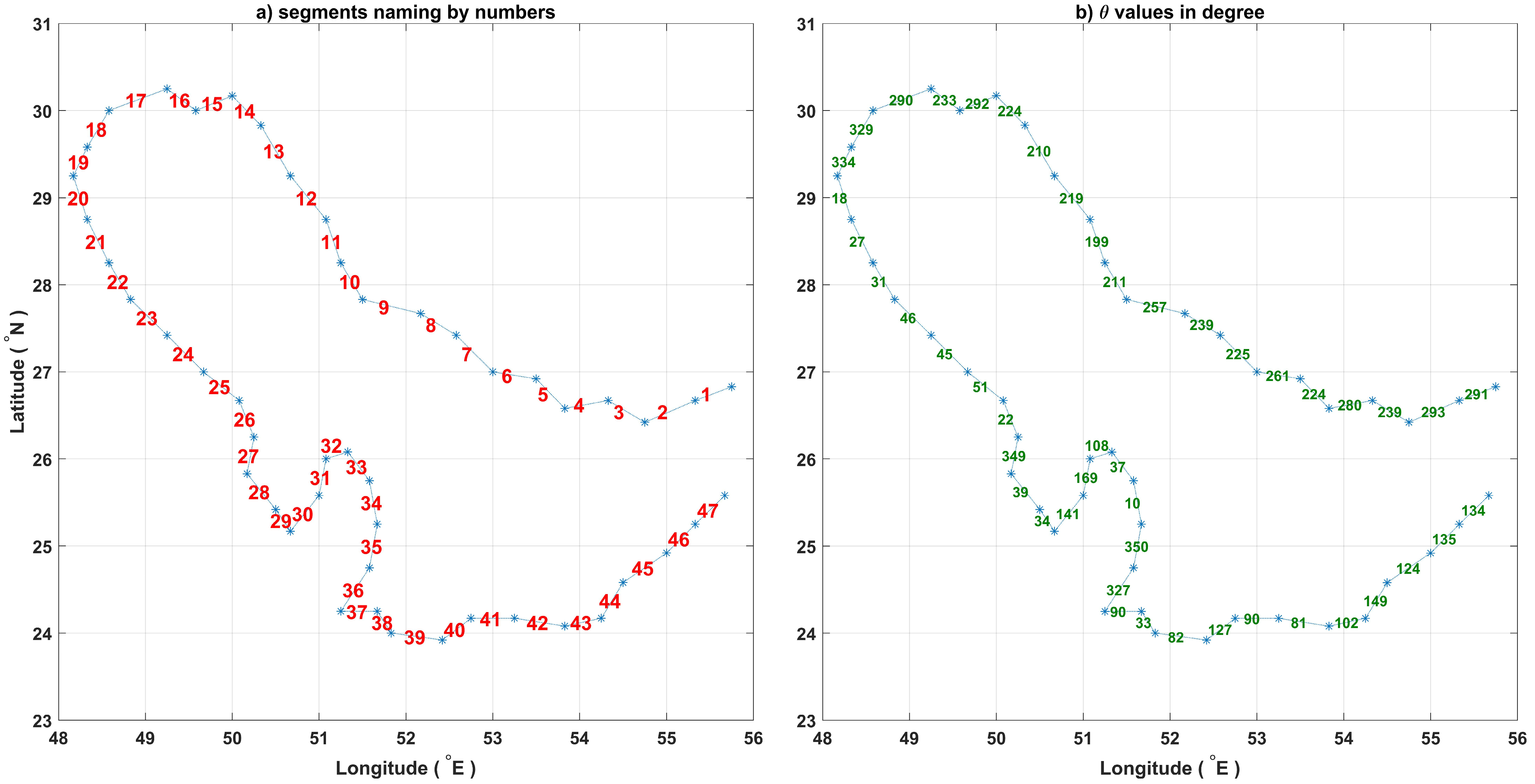
Then, the coastal area of the Persian Gulf is divided into 47 segments to study the occurrence of coastal upwelling and downwelling. These segments have been marked on the map and corresponded to data grid cells with specific latitude and longitude positions, as shown in Figure 1a.

The coastal upwelling index ($CU{I}_{Ekman}$) has been computed by determining the longitudinal (Q_x) and latitudinal (Q_y) components of Ekman transport as

$$Q_x=\frac{{\tau }_y}{{\rho }_{w}f}$$

(1)

$$Q_y=\frac{-{\tau }_x}{{\rho }_{w}f}$$

(2)

where the zonal (${\tau }_x$) and meridional (${\tau }_y$) components of wind stress are calculated from the quadratic bulk aerodynamic formulation [38], ${\rho }_w$ the sea water density (1025 kg m⁻³), and f is the Coriolis parameter (7 × 10⁻⁵ s⁻¹) [39,40]. Equation (3) has been applied to all 47 segments to estimate the coastal upwelling index [41].

$$CU{I}_{Ekman}=-Q_x\sin (\theta -\frac{\mathsf{\pi }}{2})+Q_y\cos (\theta -\frac{\mathsf{\pi }}{2})$$

(3)

In this equation, θ is the angle of the unitary vector perpendicular to the mean shoreline position and is depicted in Figure 1b for each segment. In other words, the mean shoreline position is considered for each segment, and then the angle between the oceanward vector perpendicular to the mean shoreline position and the positive part of the coordinate axis is calculated as θ.

$CU{I}_{Ekman}$ is the image of Ekman transport on the oceanward vector perpendicular to the mean shoreline position calculated in ${\mathrm{m}}^3{ \mathrm{s}}^{-1}$ by integrating along the length of the grid and detecting the coastal upwelling considering the Ekman transport intensity (Q_x, Q_y) and its direction to the shoreline (θ). This index is one of the most widely used indices of coastal upwelling, which has been used in many previous studies to investigate wind-induced coastal upwelling, such as [30,37,42].

The sign value of the Ekman transport indicates the direction of its ocean or land component. If the value is close to zero, it suggests that the dominant transport direction is oriented along the coastline. A positive value signifies favorable conditions for coastal upwelling, with a larger positive value indicating stronger upwelling. On the other hand, a negative value represents favorable conditions for coastal downwelling, with a larger negative value implying more intense downwelling [30].

For further investigation, the vertical temperature data has been obtained from the ARMOR-3D monthly dataset for 28 years (1993–2020). The data were extracted for all the coasts of the Persian Gulf in the grids with a spatial resolution of 0.25$°$ × 0.25$°$ and joined together to investigate the intra-annual cycle of vertical variability of temperature for all the segments. Additionally, the cross-shore geostrophic transport can impact the intensity of coastal upwelling and downwelling [3] which can be quantified as shown below.

Geostrophic velocities are given by

$$u_g=-\frac{g}{f}\frac{\partial h}{\partial y}$$

(4)

$$v_g=\frac{g}{f}\frac{\partial h }{\partial x}$$

(5)

The longitude and latitude are represented by x and y, respectively. The Coriolis parameter, f, has a value of 7 × 10⁻⁵ s^−1, the acceleration due to gravity, g, is 9.807 m s⁻² and the height of the sea surface relative to the geoid is represented by h [34].

The longitudinal (T_x) and latitudinal (T_y) components of geostrophic transport have been computed as follows:

$$T_{x }={{\displaystyle \int }}_{y_1}^{y_2}{{\displaystyle \int }}_{z=0}^{z}u{ }_{g }dy dz=MLD\frac{g}{f} \left(SS{H}_{north}-SS{H}_{south}\right)$$

(6)

$$T_{y }={{\displaystyle \int }}_{x_1}^{x_2}{{\displaystyle \int }}_{z=0}^{z}v{ }_{g }dx dz=-MLD\frac{g}{f} \left(SS{H}_{east}-SS{H}_{west}\right)$$

(7)

$$T_{geo}=-T_x\sin (\theta -\frac{\pi }{2})+T_y\cos (\theta -\frac{\pi }{2})$$

(8)

where $T_{geo}$ (in ${\mathrm{m}}^3{ \mathrm{s}}^{-1})$ is the image of geostrophic transport on the ocean-directed vector perpendicular to the mean shoreline. Equation (8) has been applied to estimate the total upwelling intensity in [3] improved in the present study.

To calculate $T_{geo}$, the monthly mean of sea level anomalies data by a spatial resolution of 0.25° × 0.25° has been extracted from Copernicus Marine Environment Monitoring Service (CMEMS) and monthly data of mixed layer depth from ARMOR-3D for 28 years, from January 1993 to December 2020.

Finally, $U{I}_{total} \left(\mathrm{in} m^3 s^{-1}\right) \mathrm{is} \mathrm{applied}$ to estimate the total cross-shore transport as a sum of Ekman transport ($CU{I}_{Ekman}$), and the geostrophic transport $T_{geo}$,

$$U{I}_{total}=CU{I}_{Ekman}+T_{geo}$$

(9)

$U{I}_{total}$ is applied to investigate the impact of geostrophic transport on the structure of coastal upwelling/downwelling over the Persian Gulf.

3. Results

3.1. Wind Patterns

3.1.1. Intra-Annual Variability of Wind Speed

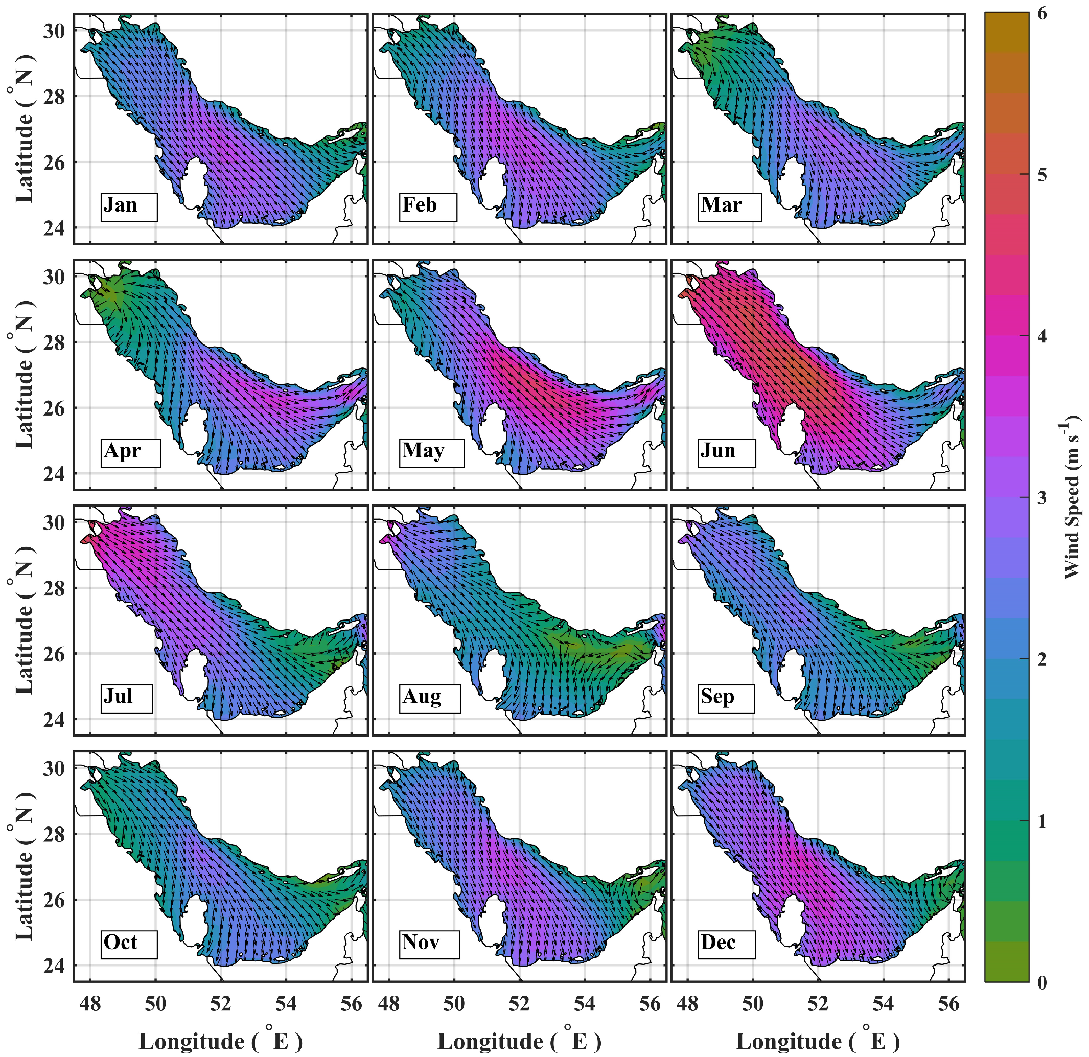
The intra-annual wind variability is displayed in Figure 2 using the 28-year hourly wind data series (in m s⁻¹). The figure illustrates the average wind speed variability for different months in the Persian Gulf over the 28-year period by representing the direction of wind speed as vectors and its intensity as the background color.

During January and February, the wind speed in the Persian Gulf is evenly and uniformly distributed in both value and direction and is stronger compared to the warmer months of August and September, but it is less intense than it is in June and July.

As spring approaches in March, the wind speed in the northwest of the Persian Gulf decreases but reaches its peak (around 3–4 m s⁻¹) along the northern coast.

In April, the wind speed has its lowest intensity and the highest variability in the direction in the northwest of the Persian Gulf. Moving towards the east, the value of the wind speed increases. During spring and early summer, the wind speed intensifies further, reaching its peak in June.

In addition, the direction of the wind is parallel to the coastline, which can provide favorable conditions for upwelling in many parts of the northern and southern coasts of the Persian Gulf in June. The value of the wind speed reduces in the warmer months of the year (August and September) and is significantly more evident in August when there is minimum intensity and the most variability in the direction of wind speed in the northern and eastern regions. However, wind speed intensifies as autumn progresses, reaching its highest value (around 4–5 m s⁻¹) in December in the center of the Persian Gulf.

3.1.2. Wind Speed EOF Analysis

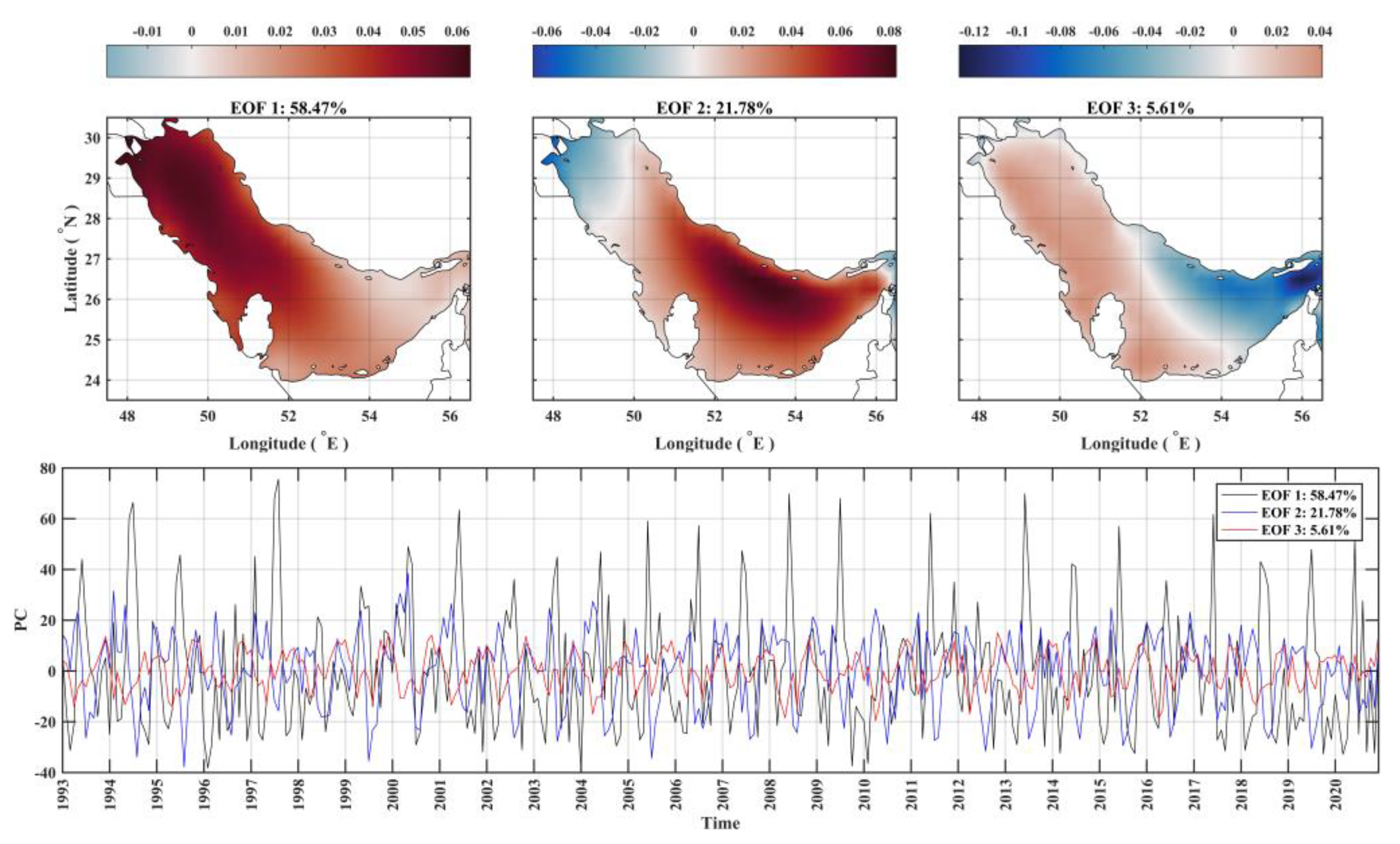
Figure 3 shows that the sum of the three leading modes explains 100% of all wind speed variance. Wind speed increases (decreases) during positive (negative) PC time in regions with positive EOF. Subsequently, it decreases (increases) during positive (negative) PC in regions with negative EOF. Each mode shows the dominance of these variabilities in the time series, corresponding to the eigenvalue value. The EOF 1 (first mode of wind speed EOF analysis), with the eigenvalue of 68.1%, is the leading EOF for the wind speed, which is a uniform mode with all positive counters and represents a spatially coherent increase/decrease of wind speed over the entire basin.

In other words, the contribution of EOF 1 is to increase/decrease the wind speed extremes over the Persian Gulf (spatially in the northwest part of the Persian Gulf when the PCs are positive/negative) [43]. According to the first leading time series (PC-EOF 1: black line in Figure 3), in the first months (winter) of all the years, the PCs are negative and show that the wind speed decreases throughout the Persian Gulf in winter, but in following months the PCs are positive and show that during spring and early summer, the wind speed increases throughout the Persian Gulf. The EOF 1 also exhibits dominance with maximum intensity in the northwest part of the Persian Gulf, spreading and waning toward the central and southeast.

The maximum positive intensity of PC in the wind speed is observed during a few years, including 1997, 2008, 2009, and 2013. These fluctuations correspond to tropical storms and cyclones such as Gonu, Phet, and Ashobaa that occurred in the Arabian Sea in June. During a cyclone, the atmosphere and the ocean are constantly exchanging energy.

The second leading mode, with an eigenvalue of 25.37% (PC-EOF 2: blue line in Figure 3), display three meridian bands of acting centers, one positive anomaly (central) between two negative (east and northwest) anomalies. The contribution of this mode is to increase/decrease wind speed in the central and southeast Persian Gulf and simultaneously decrease/increase wind speed in the east and northwest Persian Gulf according to the amplitude of the PC. According to the PC-EOF 2, the PCs are positive in the first months of the year (winter) over the time series. It shows that the wind speeds increase (decrease) in the central and southeast (northwest) of the Persian Gulf in winter.

Finally, the third leading mode of wind speed (PC-EOF 3: red line in Figure 3) with an eigenvalue of approximately 6.53%, displays a dipole pattern where the positive (negative) anomalies occur on the west (east) part of the Persian Gulf. In other words, an imaginary line divides the Persian Gulf into two eastern and western parts.

According to the PC-EOF 3, the PCs are positive in the early winter, summer, and autumn over the time series. This shows that the wind speed increased (decreased) in the west (east, spatially near the Strait of Hormuz) part of the Persian Gulf during these periods. The PCs are negative in the second and third months of the winter and spring over the time series. It shows that the wind speed increased (decreased) in the west (east, spatially near the Strait of Hormuz) part of the Persian Gulf during these periods.

3.2. Ekman Transport

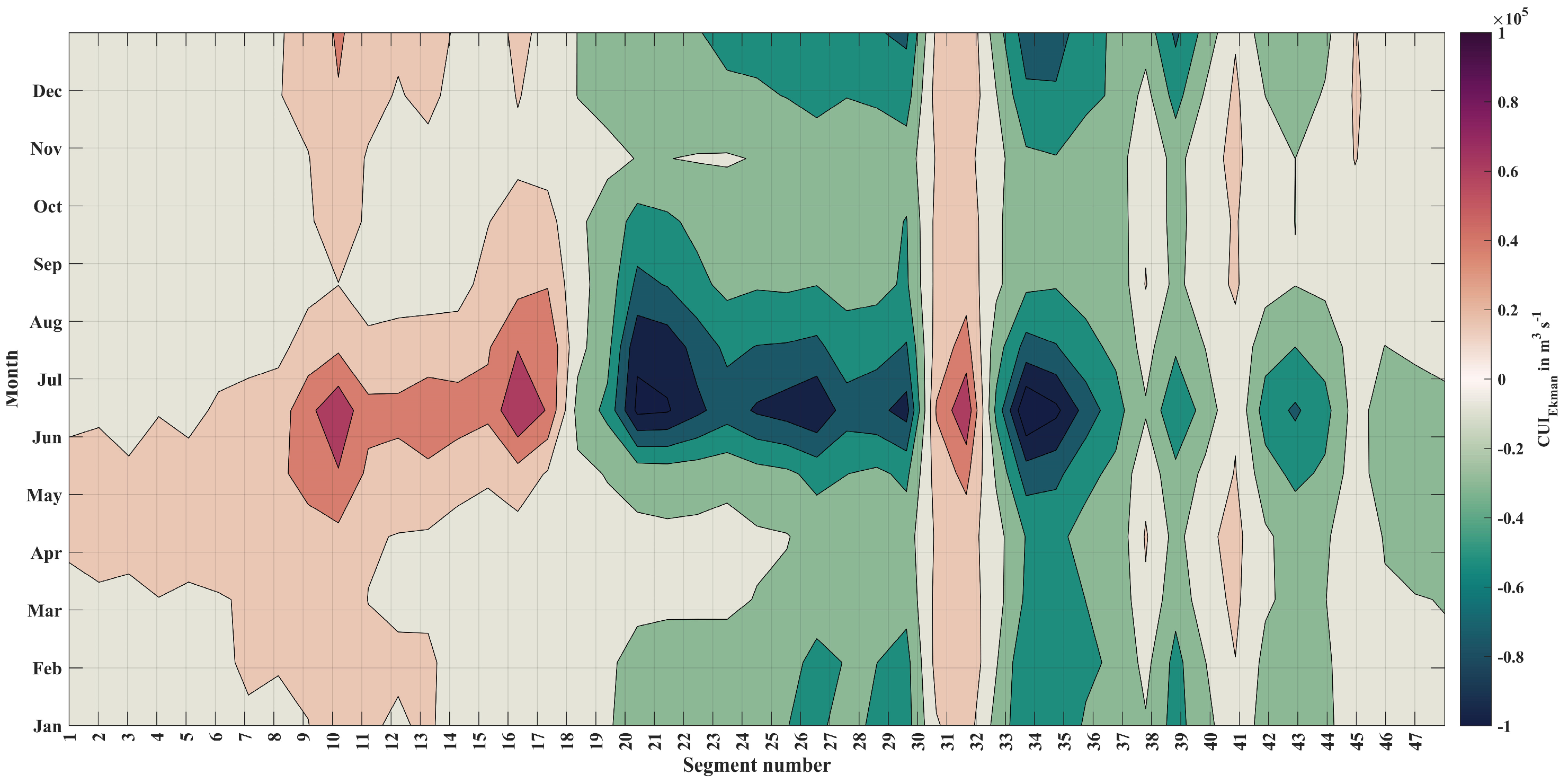
The daily $CU{I}_{Ekman}$ time series for the 47 segments has been calculated using the wind data series for over 28 years, from 1993 to 2020. The monthly mean annual cycle of $CU{I}_{Ekman}$ is depicted in Figure 4.

The $CU{I}_{Ekman}$ values are positive and negative (Figure 4). However, the segments in some regions are more significant. Segments 10–11 (around 51.5$° \mathrm{E}$ and 28$° \mathrm{N})$, 16–17 (around 49$° \mathrm{E}$ and 30$° \mathrm{N})$, and 31–32 (around 51$° \mathrm{E}$ and 26$° \mathrm{N})$, have the most intense coastal upwelling. The coastal upwelling occurred with different intensities over a year at these segments, but there is a peak in June. By distancing from these segments or the peak, spatially or temporally, the positive value of $CU{I}_{Ekman}$ (corresponding to upwelling) decreases and the intensity of coastal upwelling is reduced.

Furthermore, as seen in Figure 4, some segments have negative $CU{I}_{Ekman}$ values, which indicates a landward direction for the Ekman transport [30]. Negative values of $CU{I}_{Ekman}$, correspond to favorable downwelling conditions, with a more negative value indicating stronger downwelling. However, the segments in some regions are more significant. The segments 20–22 (around 48$° \mathrm{E}$ and 29$° \mathrm{N}-49 ° \mathrm{E} \mathrm{and} 28 ° \mathrm{N})$, 26–27 (around 50 $° \mathrm{E}$ and 26$° \mathrm{N})$, 29–30 (about 50.5 $° \mathrm{E}$ and 25.5$° \mathrm{N})$, and 33–35 (around 51.5 $° \mathrm{E}$ and 26$° \mathrm{N}-51.5 ° \mathrm{E} \mathrm{and} 25 ° \mathrm{N})$, have the most intense downwelling.

There are positive $CU{I}_{Ekman}$ values in segments 1 to 18 (along the northern coast of the Persian Gulf), with the highest values being in segments 9 to 18 in spring–summer and a peak in segments 16 and 16–17 in June. $\mathrm{The} CU{I}_{Ekman}$ has negative values throughout segments 19 to 30 (along the northwestern and western coast of the Persian Gulf), with the highest values being in spring, summer, and the late fall, with a peak in June.

$\mathrm{In} \mathrm{addition}, \mathrm{the} CU{I}_{Ekman}$ has positive values throughout segment 31 (along the southern coast of the Persian Gulf), with the highest values being in May–July and a peak in June. Finally, $\mathrm{The} CU{I}_{Ekman}$ has negative values in almost segments 32 to 48 (along the southern and southwestern coast of the Persian Gulf), with the highest values being in spring, summer, and the late fall in segments 33 to 35, with a peak in June.

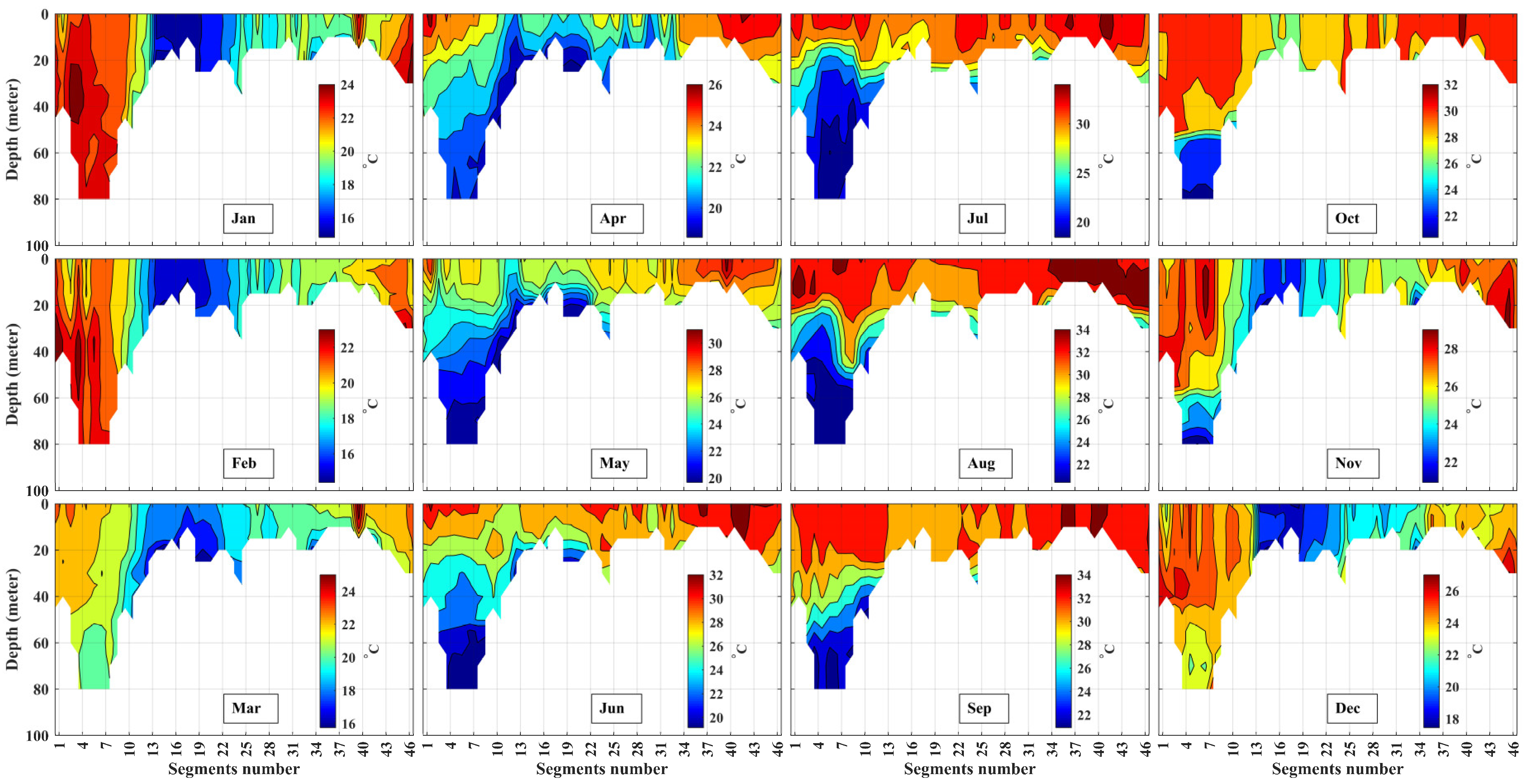
3.3. Intra-Annual Vertical Variability of the Temperature

The intra-annual vertical variability in temperature is displayed in Figure 5 using the monthly temperature data series over 28 years from 1993 to 2020.

According to Figure 5, there is the lowest difference between the temperature of the surface and bottom in January and February during the year in each segment (1 °C or less) on the northern coast of the Persian Gulf, which is the deepest coastal part of it (segments 1 to 16). This difference increases towards the warmer months and reaches 14 °C in July and August. The surface temperature varies between 14 °C and 34 °C in January and February in segments 13 to 16 and July/Aguste in segment 7, respectively, while the temperature of the bottom remains constant at 20 °C in most of the spring, summer, and fall months in segments 4 to 7 and it has the minimum value about 14 °C in January and February in segments 10 to 13.

Also, there is a significant difference between the temperature of the surface and bottom in spring and summer during the year in each segment, so it reaches the maximum value in July and August on the northwest coast of the Persian Gulf (segments 16 to 25), while the temperature of the water column remains constant in fall and winter in each segment. The surface temperature varies between 15 °C and 32 °C in January and February in segments 16 to 19 and July/Aguste in segments 17 to 25, respectively, and the temperature of the bottom changes between 15 °C and 29 °C in January and February in segments 16 to 19 and October in segment 24, respectively.

In addition, there is a difference between the temperature of the surface and on the southern and bottom southeast coasts of the Persian Gulf, while the temperature of the water column remains almost constant over the year in segments 34 to 40, which is the shallowest coastal part of the Persian Gulf. The surface temperature varies between 19 °C and 34 °C in January and February in segments 25 to 28 and July and September in segments 36 and 41, as well as in segments 33 to 42 in Aguste, respectively, and the temperature of the bottom changes between 16 °C and 34 °C in January in segment 34 and Aguste and September in segments 35 and 36, respectively.

The vertical temperature variability in the surface and the bottom layers changes over different seasons. The seasonal thermocline over the coasts of the Persian Gulf is formed in spring and intensified in summer but weakens and finally disappears in autumn and winter. In June, when there is the most favorable condition for the upwelling, the mixed layer depth is larger than others in segments 10–11. The thermocline becomes deeper, as a result. Additionally, the lowest vertical gradient of temperature is in this area. In other words, according to Figure 5, there is a lower temperature difference between the surface and the bottom at segments 10–11 in June.

3.4. Geostrophic Transport

The daily $T_{geo}$ time series for the 47 segments was calculated for 28 years (1993–2020) using Equations (6)–(8), and its monthly average annual pattern is displayed in Figure 6. The $T_{geo}$ values are positive and negative (Figure 6), so these positive and negative values are scattered throughout the coasts of the Persian Gulf and during all months of the year.

The highest accumulation of maximum geostrophic transport values towards the onshore region (negative) and offshore region (positive) are in the northeastern areas of the Persian Gulf.

In the northern part of the Persian Gulf (segments 1–16), there is geostrophic transport towards the onshore region in winter which occurs in segments 6 and 9. This transport continues in segment 6 until June but stops in late February in segment 9. Geostrophic transport has a positive value in segments 3 to 10. Segments 3, 5, 11, and 13 have trivial geostrophic transport values, while in other segments, there is no significant geostrophic transport during these three months. In the spring, geostrophic transport has a positive value in segment 3 around April, while its values are negligible in segments 10 to 16. Additionally, it has a significant negative value in segment 7, and a trivial in segment 5 during June. There is no considerable geostrophic transport in other segments. In summer, in segment 7, there is significant geostrophic transport towards the onshore region in July, which decreases in August and September. In addition, geostrophic transport towards the onshore region occurs in sections 11 and 4, so it decreases as it progresses toward its surrounding areas and reaches a negligible value. Geostrophic transport towards the offshore region exists during these three months in segment 1, so it attains a maximum value in August. In autumn, segments 1 and 3 have significant geostrophic transport towards the offshore region, which reaches its maximum value in November. Meanwhile, between these two segments (segment 2), the highest value of geostrophic transport towards the onshore region occurs in November. Furthermore, segments 6 and 11 (7, 10, and 13) have geostrophic transport towards the onshore (offshore) region during these three months.

In the northwestern part of the Persian Gulf, there is geostrophic transport towards the onshore region in segments 20 to 22 in winter (January–March) so that attains the maximum value in February in segment 21, while there is geostrophic transport towards the offshore region in segment 17 with a maximum value in January so that reduces towards the spring. In spring (April–June), there are insignificant amounts of geostrophic transport towards the onshore region in segments 21 to 25. The other segments have no significant geostrophic transport on the northwestern part of the Persian Gulf. In summer (July–October), there is geostrophic transport towards the onshore region in segments 17 to 19 so that attains the maximum value in Aguste in segment 17. In the fall (September–December), geostrophic transport towards the offshore region is commenced in October and intensifies towards the winter so that reaches the maximum value in early January in segment 17. Segments 21 to 25 exhibit positive geostrophic transport in the fall, with a maximum value in October in segment 25, while segments 19 and 20 have negative geostrophic transport. As a result, segment 19 (20) reaches a maximum value in October (late December).

In the southern and southern east part of the Persian Gulf (segments 25–48), there is onshore geostrophic transport in winter, which occurs in segments 35 and 47, and continues in segment 35 until September. The geostrophic transport has a positive value in segments 28 and 47 and attains its maximum value in March and May (June) in segment 28 (47). Segments 39 to 41 have negligible positive geostrophic transport values, while in other segments, there is no significant geostrophic transport during these three months. In spring, geostrophic transport has a positive value in segment 28 around May, while its values are negligible in segments 39 and 41. Additionally, it has a significant negative value in segments 33 and 34. In summer, there is onshore geostrophic transport in segment 33. In addition, geostrophic transport towards the onshore (offshore) region occurs in segments 43 to 47 (35, 36, and 38). In the fall, there is no significant geostrophic transport towards the offshore region, while segments 35 to 37 (44 to 47) have the highest onshore geostrophic transport in late December (November) during these three months.

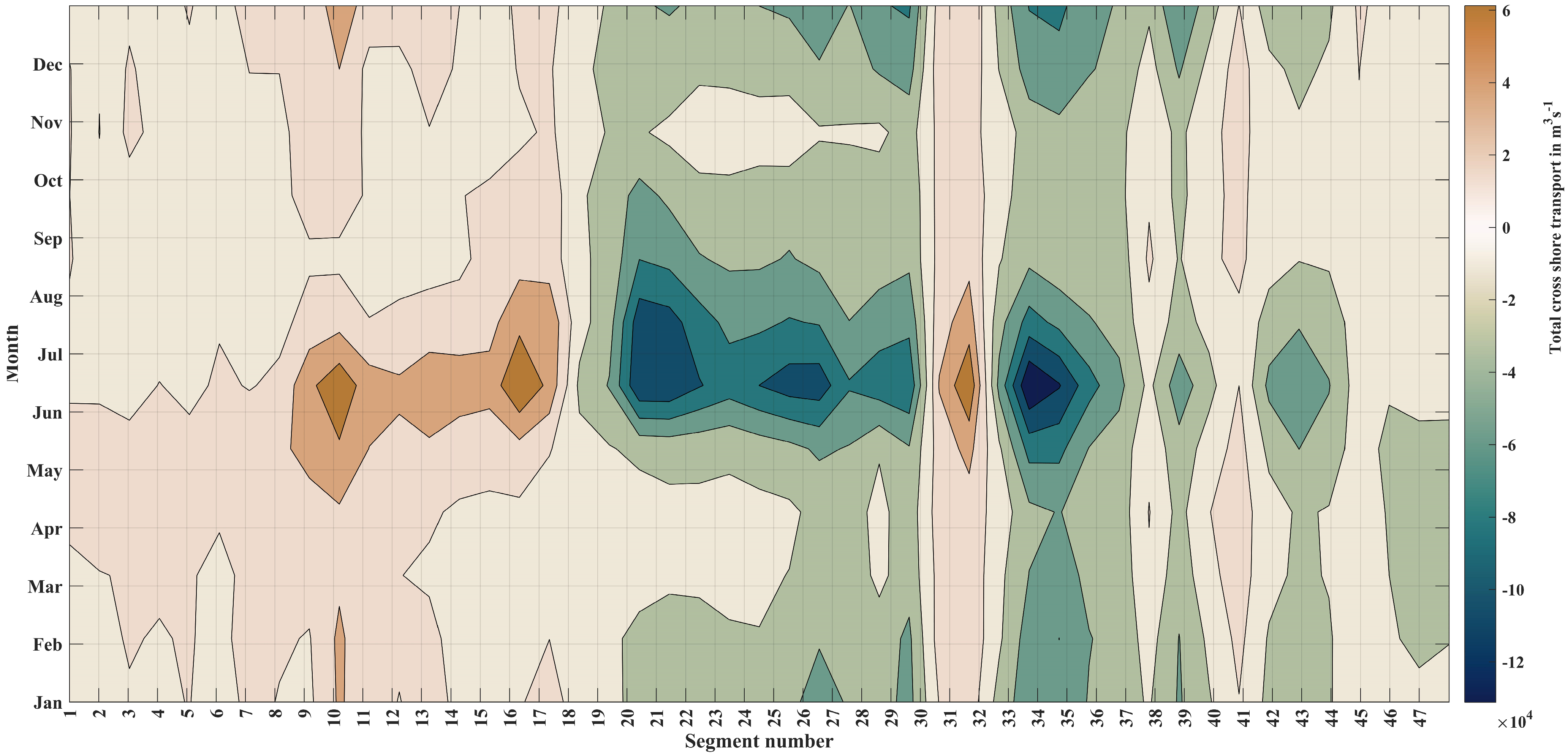
3.5. The Effect of Ekman and Geostrophic Transport Components on Total Cross-Shore Transport Corresponding to Upwelling/Downwelling

The daily $U{I}_{\mathrm{total}}$ time series covering 28 years (1993–2020) was calculated for the 47 segments using Equation (9), and its monthly mean annual cycle is displayed in Figure 7.

The $U{I}_{total}$ values are positive (corresponding to upwelling) and negative (corresponding to downwelling). However, the segments in some regions are more significant. Segments 10 (around 51.5 $° \mathrm{E}$ and 28$° \mathrm{N})$, 16–17 (around 49$° \mathrm{E}$ and 30$° \mathrm{N})$, and 31–32 (around 51$° \mathrm{E}$ and 26$° \mathrm{N})$, have the most intense coastal upwelling. The coastal upwelling occurred with different intensities over a year at these segments, but there is a peak in June. By distancing from these segments or the peak, spatially or temporally, the positive value of $U{I}_{total}$ decreases and the intensity of coastal upwelling reduces.

In addition, $U{I}_{total}$ values are negative in some segments. However, the segments in some regions are more significant. Segments 20–22 (around 48$° \mathrm{E}$ and 29$° \mathrm{N}–49 ° \mathrm{E} \mathrm{and} 28 ° \mathrm{N})$, 26–27 (around 50$° \mathrm{E}$ and 26$° \mathrm{N})$, and spatially, 33–35 (around 51.5$° \mathrm{E}$ and 26$° \mathrm{N}–51.5 ° \mathrm{E} \mathrm{and} 25 ° \mathrm{N})$, have the most intense downwelling.

According to Figure 5 and Figure 7, the total cross-shore transport pattern is very similar to the $CU{I}_{ekman}$ in terms of spatial and temporal structure, and it accurately identifies the same segments as active upwelling and downwelling regions and shows the same favorable time conditions for the formation of these phenomena. Therefore, the Ekman transport is the dominant component in the total cross-shore transport, which can accurately determine the structure of active upwelling and downwelling in the Persian Gulf, but the geostrophic transport affects the intensity of upwelling and downwelling.

According to Figure 4, the maximum value of the $CU{I}_{ekman}$ is about 0.8 × 10⁵ ${\mathrm{m}}^3{ \mathrm{s}}^{-1}$ in segments 10, 19, and 32, but the maximum value of the $U{I}_{total}$ decreases to about 6 × 10⁴ ${\mathrm{m}}^3{ \mathrm{s}}^{-1}$ in these segments, which shows that the intensity of upwelling decreases by considering the geostrophic transition in the upwelling/downwelling index. Additionally, the maximum absolute value of $T_{geo}$ is about 1 × 10⁵ ${\mathrm{m}}^3{ \mathrm{s}}^{-1}$ in segments 10, 19, and 32, while the maximum absolute value of $U{I}_{total}$ increases to about 12 × 10⁴ ${\mathrm{m}}^3{ \mathrm{s}}^{-1}$ in these segments, which indicates that the intensity of downwelling increases by considering the geostrophic transport in the upwelling/downwelling index in these areas. In other words, with the algebraic sum of geostrophic and Ekman transport, the intensity of the coastal upwelling decreases, and the intensity of the coastal downwelling increases in the favored spatial and temporal conditions in the Persian Gulf.

4. Discussion

Figure 2 displays the intra-annual variability of wind data over 28 years using the hourly wind data. It shows that the wind in the Persian Gulf is strong and evenly uniformly distributed (both value and direction) during January and February, and it is more intense than in the warmer months of August and September but is less intense than in June and July. The reason for this behavior is that the winter Shamal blows from the northwest during the cold months of the year and commonly generates significant dust storms, spreading to the southeast and covering the entire Persian Gulf [25]. The northern part of the Persian Gulf in Iran is especially prone to dust storms [44].

As spring approaches in March, wind speed decreases in the northwestern regions of the Persian Gulf, but the northern coast of the Persian Gulf experiences the highest wind speeds (around 3–4 ms⁻¹) during this month. This region near Ra’s-e-Motaf is known as Iran’s Bermuda triangle for its frequent storms and many sunken ships and has the highest wave energy levels in the Persian Gulf [45].

In April, the wind speed in the northwest of the Persian Gulf has the lowest intensity and the greatest variability (in the direction). Moving towards the east, the wind speed increases. During spring and early summer, the wind speed intensifies, reaching its peak in June due to the prevalent summer Shamal wind in the area [25,46]. In autumn, the wind speed continues to rise, reaching its highest value (around 4–5 ms⁻¹) in December in the center of the Persian Gulf. This central region exhibits greater monthly variability in wind speed compared to other areas [45].

According to Figure 3, EOF 1 corresponds to the summer Shamal and presents the leading wind pattern in the Persian Gulf because the winter Shamal has a greater intensity in the central region while, during the summer Shamal, the highest wind speeds move to the northern area according to the results presented by [31,47].

The maximum positive intensity of PC in the wind speed occurred during a few years, including 1997, 2008, 2009, and 2013. These fluctuations correspond to tropical storms and cyclones such as Gonu, Phet, and Ashobaa that occurred in the Arabian Sea in June. During a cyclone, the atmosphere and the ocean are constantly exchanging energy. The cyclone-induced tensions push the ocean to the marginal shores, trigger storm surges on the northeast coast of the Arabian Sea, and swell waves play a vital role in the formation of higher wave heights during this time [48]. so that its effects extend to the Gulf of Oman and the Persian Gulf. These factors increase the wind speed along with the summer Shamal in the Persian Gulf [49,50,51,52,53].

The second leading mode shows that the wind speed increased (decreased) in the central and southeast (northwest) of the Persian Gulf in winter. The winter Shamal is stronger in the central region, according to the results presented by [31,47]. Therefore, EOF 2 corresponds to the winter Shamal and represents one of the leading wind patterns in the Persian Gulf.

Finally, the third leading mode of wind speed displays a dipole pattern where the positive (negative) anomalies occurred in the western (eastern) region of the Persian Gulf. This difference in the wind pattern in the eastern and western parts of the Persian Gulf, indicated in the third leading mode, can be caused by the effects of external factors, such as the winds, storms, and monsoons that reach the Strait of Hormuz from the Arabian Sea and the Gulf of Oman. Their effects spread to the central parts of the Persian Gulf.

The fact that the imaginary line crosses the PC-EOF 3’s dipole suggests that the variability accounted for this mode could have a marine origin associated with the return flow to the southeast. The prevailing wind direction is the opposite of the inflow from the Strait of Hormuz to the Persian Gulf. Therefore, these shallow regions become weaker [24].

This mode is less significant in the discussion than in the first and second modes due to the small contribution to the variance in the surface wind speed of the region. So, the PC-EOF 1 have significant importance, the wind dynamics were closer to unimodality, and the effect of only external factors, such as the winds, storms, and monsoon that reach the Strait of Hormuz from the Arabian Sea and the Gulf of Oman, is, generally, smaller than the effect of external factors such as seasonal change, during the studied period, as a result. It should be mentioned that the combination and simultaneity of internal and external factors can increase wind speed.

The daily $CU{I}_{Ekman}$ time series for the 47 segments over 28 years (1993–2020) has been computed using the wind data time series. The monthly mean annual cycle of these computations presents in Figure 3. However, the segments in some regions are more significant. Segments 10–11 (around 51.5$° \mathrm{E}$ and 28$° \mathrm{N})$, 16–17 (around 49$° \mathrm{E}$ and 30$° \mathrm{N})$, and 31–32 (around 51$° \mathrm{E}$ and 26$° \mathrm{N})$, have the strongest coastal upwelling with a peak in June. The probability of significant coastal upwelling at the region of about 51.5$° \mathrm{E}$ and 28$° \mathrm{N}$ had been already reported by [30], who investigated wind-driven coastal upwelling along the northern shoreline of the Persian Gulf and showed the strongest coastal upwelling in the central areas of the northern shoreline of the Persian Gulf, located in about 51° E–53° E.

As shown by [31], the upwelling effects in the area close to the coast of Kuwait are at about 49$° \mathrm{E}$ and 30$° \mathrm{N}$. Furthermore, according to Figure 4, in the area of about 51$° \mathrm{E}$ and 26$° \mathrm{N}$, there is a possibility of favorable conditions for the coastal upwelling.

On the other hand, the probability of significant coastal upwelling in June had already been reported by [30,54], who inferred that the thermocline develops, particularly in the northern Persian Gulf in the summer, and increases the chances of upwelling. This is due to the influence of the prevailing Shamal winds in the area during June [25,34,46]. Additionally, the impact of monsoon waves generated during the monsoon season on the southern coastline of the Arabian Peninsula in the Indian Ocean, which approach from the south, may also contribute to the maximum value of the coastal upwelling index in June in this area [10].

During summer, many coastal regions experience a shift in wind direction due to the seasonal change in atmospheric pressure, which results in variability in the direction of surface winds [5]. In the Persian Gulf, this change in wind direction with the intensification of the Shamal winds leads to the onset of coastal upwelling.

Furthermore, a negative value of the Ekman transport indicates a component that moves towards the land [30]. Therefore, using the $CU{I}_{Ekman}$, negative values correspond to favorable downwelling conditions, and the more negative value implies a stronger downwelling so, the segments 20–22 (around 48$° \mathrm{E}$ and 29$° \mathrm{N}-49° \mathrm{E} \mathrm{and} 28° \mathrm{N})$, 26–27 (around 50$° \mathrm{E}$ and 26$° \mathrm{N})$, 29–30 (around 50.5$° \mathrm{E}$ and 25.5$° \mathrm{N})$, and 33–35 (around 51.5$° \mathrm{E}$ and 26$° \mathrm{N}-51.5 ° \mathrm{E} \mathrm{and} 25° \mathrm{N})$, have the most intense downwelling.

According to Figure 4, there is a favorable condition for the occurrence of downwelling in the second and fourth regions but seems that due to the shallow depth of these areas, it does not have any special physical effects, so there is a probability of significant downwelling in two regions (segments 20–22 and 29–30).

Downwelling occurred with varying strengths over a year at these segments, but there is a peak in June. In other words, not only are favorable conditions engendered by the creation of upwelling, but in other areas, downwelling can occur in June as well. Moving away from these segments or the peak, either spatially or temporally, the negative value of $CU{I}_{Ekman}$, (corresponding to downwelling) decreased and the intensity of downwelling is reduced.

According to Figure 5, the seasonal thermocline over the coasts of the Persian Gulf forms in the spring and intensified in the summer but, weakens and finally disappears in autumn and winter.

During the hot season, the upper layer of the Persian Gulf has a warm temperature profile, with temperatures typically ranging from 28 to 34 °C at the surface to around 22–25 °C at a depth of 50 m. This warm upper layer is primarily due to the high solar radiation and the lack of significant cooling from the surrounding land areas. It leads to a strong thermocline that separates the warm surface layer from the colder and deeper layer.

However, in areas of the Persian Gulf that are very shallow, such as segments 35 to 42 (less than 20 m deep), the water column temperature remains constant in summer, particularly in August. It prevents the formation of a thermocline during this month due to the small depth of the area.

The high air temperature transfers to the water surface, causing the water column to mix, resulting in an insignificant difference between surface and bottom temperature.

As a result, the bottom temperature remains high at 34 °C, which endangers the marine plant and animal species in this area.

During the cold season, the upper layer of the Persian Gulf has a colder temperature profile, with temperatures typically ranging from 20 to 24 °C at the surface to around 15–18 °C at a depth of 50 m. This cooler upper layer is primarily due to the cooler air temperatures over the surrounding land areas and the influence of colder air masses from the north. The thermocline can also become weaker during the cold season, allowing for more mixing between the upper and deeper layers of the Persian Gulf.

The systems of middle latitudes weather can affect the Persian Gulf thermocline by altering the wind patterns and surface heat fluxes. During the winter months, the systems of middle-latitude weather can bring strong northwesterly winds to the Persian Gulf. These winds can increase the mixing of the water column and weaken the thermocline, allowing for more mixing between the upper and deeper layers of the Persian Gulf. It can lead to a decrease in the strength of the thermocline and a more uniform temperature profile throughout the water column.

On the other hand, during the summer months, the systems of middle-latitude weather can bring southeasterly winds to the region. It can reduce the mixing of the water column and strengthen the thermocline. It can cause a more distinct separation between the warm surface to the bottom.

By applying northwestern wind in winter, the fresher inflow can penetrate much further into the Persian Gulf. The lack of wind-induced mixing and solar radiation leads to thermocline formation and its development from winter to summer [55].

In June, when conditions for the coastal upwelling are the most favorable (Figure 4), the mixed layer depth is larger than others in segments 10–11. The thermocline becomes deeper, as a result. Additionally, there is the lowest vertical gradient of temperature in this area. In other words, according to Figure 5, there is a lower temperature difference between the surface and the bottom in segments 10–11 in June. When strong coastal upwelling occurs, its physical quantities and dynamic conditions are affected by this physical phenomenon. The Ekman Current, from onshore to offshore areas with vertical pumping, causes the mixing of the water column and reduces the temperature difference between the surface and the bottom in this area. Moreover, the pumping of cold water from the lower layers to the surface is visible, so the surface temperature of these segments decreases compared to the eastern and western parts around them. The two other segments, with the possibility of the coastal upwelling, do not exhibit these special physical effects due to the shallowness. As a result, the most favorable condition for the upwelling is in segments 10–11 in June.

According to Figure 6, the highest accumulation of maximum geostrophic transport values towards the onshore (negative) and offshore (positive) occurred in the northeastern regions of the Persian Gulf. This accumulation causes by differences in surface density due to the influx of less salty water into the Persian Gulf through the Strait of Hormuz. This effect causes by the outflow-inflow of dense water through the Strait of Hormuz and strong stratification. The influx of warmer and fresher water through the Strait of Hormuz can disrupt the cross-shelf density field and initiate the baroclinic instability process [25].

In the northwestern part of the Persian Gulf (segments 18 and 19), there is also a maximum offshore geostrophic transport towards the late fall and winter. The difference in surface density results from the inflow of freshwater through river discharges, mainly in late fall and winter. This freshwater inflow increases the surface density in the Persian Gulf and causes the highest offshore geostrophic transport in these areas. Elsewhere along the northern coast of the Persian Gulf, there is often geostrophic transport towards the onshore (offshore) in warm (cold) months. In the southeastern part of the Persian Gulf (segments 46 and 47), due to its proximity to the Strait of Hormuz, there is a maximum value of geostrophic transport, which is towards the offshore region in the summer, and towards the onshore region in the colder months.

Furthermore, there is a maximum value of geostrophic transport towards the offshore region in segments 25–26 in the autumn months and in segments 28–29 in the late winter and spring months. There is a significant value of geostrophic transport toward the onshore region from January to September in segments 33–36, as well.

According to Figure 4 and Figure 6, the intensity of the cross-shore Ekman transport is higher than the geostrophic transport over the coasts of the Persian Gulf, which indicates the dominance of this transport component due to the presence of the prevailing wind and the influence of wind stress on the surface currents. In the Persian Gulf, the geostrophic transport is generally weaker than the Ekman transport due to the shallow depth of the basin, the shallowness of the mixed layer depth, and the relatively weak Coriolis force in the region.

Finally, according to Figure 7, the intensity of the coastal upwelling decreases, and the intensity of the coastal downwelling increases in the favorable spatial and temporal conditions in the Persian Gulf by considering the geostrophic transport in the upwelling/downwelling index.

The geostrophic transport in the Persian Gulf may modify the direction and speed of the surface currents. These currents can oppose the offshore Ekman transport, reducing the intensity of upwelling in the region.

According to Equation (9), the geostrophic transport has been obtained from the geostrophic component of the sea surface current, and the Ekman transport corresponds to the Ekman component of the sea surface current. According to Figures 1 and 2 in [34], the direction of the Ekman components is from northwest to south and southeast in June so that they flow parallel and in the same direction throughout the Persian Gulf, but the direction of the geostrophic components, which is one of the main factors in the formation of eddies in the Persian Gulf, is variable over the domain. This current component causes a counter-clockwise rotation in the Persian Gulf, so it flows from east to west on the northern coasts and from west to east on the southern coasts of the Persian Gulf. This variability in the directions of the two components causes the image of their transport on the oceanward vector perpendicular to the mean shoreline position to change in different areas of the northern and southern coasts. So, the two components transport in the cross-shore direction, strengthen each other in some places, and weaken each other in other places.

Geostrophic transport and eddy activities interact and influence each other, shaping ocean circulation and playing a role in the transport of heat and water masses, so coastal upwelling and mesoscale eddies are considerable cyclic phenomena [34].

As a result, it will be useful to investigate the mechanism of mesoscale eddies activity, the interaction of mesoscale eddies and upwelling/downwelling, and their effects on the physical characteristics of the Persian Gulf.

5. Conclusions

This study analyzes the patterns of wind-driven coastal upwelling/downwelling in the Persian Gulf and evaluates the impact of geostrophic transport on these processes by reviewing long-term time series data. The key findings can be summarized as follows:

-

The strong and uniformly distributed wind (both value and direction) in the Persian Gulf during January and February has a greater intensity than in August and September, but it is less intense than in June and July. In many parts of the northern and southern coasts of the Persian Gulf, the direction of the wind is parallel to the coastline, which can provide favorable conditions for upwelling and downwelling in June. PC-EOF 1 has significant importance, the wind dynamics are closer to unimodality, and the effect of external factors, such as the winds, storms, and monsoon that reached the Strait of Hormuz from the Arabian Sea and the Gulf of Oman, is generally smaller than the effect of internal factors such as seasonal change during the studied period, as a result. It should be mentioned that the combination and simultaneity of internal and external factors can increase wind speed. The segments in some regions are more significant coastal upwelling index, but segments 10–11 (about 51.5$° \mathrm{E}$ and 28$° \mathrm{N})$, 16–17 (about 49$° \mathrm{E}$ and 30$° \mathrm{N})$, and 31–32 (about 51$° \mathrm{E}$ and 26$° \mathrm{N})$ have the most intense coastal upwelling, and there is a peak in June due to the effect of Shamal winds and monsoon waves, which prevails in the area during that month. Segments 20–22 (about 48$° \mathrm{E}$ and 29$° \mathrm{N}-49° \mathrm{E} \mathrm{and} 28° \mathrm{N})$, 26–27 (around 50$° \mathrm{E}$ and 26$° \mathrm{N})$, 29–30 (around 50.5$° \mathrm{E}$ and 25.5$° \mathrm{N})$, and 33–35 (around 51.5$° \mathrm{E}$ and 26$° \mathrm{N}-51.5° \mathrm{E} \mathrm{and} 25° \mathrm{N})$, have the most intense downwelling with a peak in June as well.

-

In June, when conditions are the most favorable, for the upwelling, the mixed and thermocline layer is deeper than others in segments 10–11. Additionally, the pumping of cold water from the lower layers to the surface is visible, and the surface temperature of these segments decreases compared to the eastern and western parts around them, so the most favorable condition for the upwelling is in June at segments 10–11.

-

The highest accumulation of maximum geostrophic transport values towards the onshore regions (negative) and the offshore regions (positive) are in the northeastern areas of the Persian Gulf due to the difference in surface density in these areas because of the entry of less salty water inflow through the Strait of Hormuz to the Persian Gulf.

-

The northwestern part of the Persian Gulf experiences a peak in geostrophic transport towards the offshore area due to variations in surface density caused by the influx of freshwater from river discharges during late autumn and winter.

-

The cross-shore Ekman transport surpasses the geostrophic transport along the coasts of the Persian Gulf, demonstrating the greater influence of this transport mechanism owing to the prevalence of winds, a shallow mixed layer depth, and the relatively weak Coriolis force in the region. The intensity of the coastal upwelling decreases, and the intensity of the coastal downwelling increases in the favorable spatial and temporal conditions in the Persian Gulf by considering the geostrophic transition in the upwelling/downwelling index.

-

The limited and discontinuous observational data are one of the limitations of studies in the Persian Gulf, so it is recommended to investigate the interaction of mesoscale eddies and upwelling/downwelling and their effects on the physical characteristics of the Persian Gulf through an analysis of the outputs of the numerical simulations.