
E-Learning Proposal for 3D Modeling and Numerical Simulation with FreeFem++ for the Study of the Discontinuous Dynamics of Biological and Anaerobic Digesters

 , , and
Abstract
:1. Introduction
2. Materials and Methods
2.1. Governing Equations
2.1.1. Stokes Equations
2.1.2. Advection–Diffusion Equation (ADE)
2.1.3. Diffusion Reaction Equation (DRE)
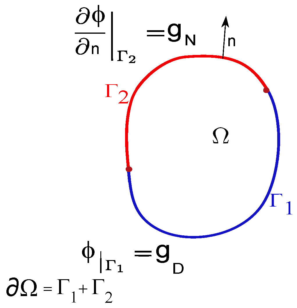
2.2. Boundary and Initial Conditions
2.3. Implementation of ADM1
2.4. Numerical Method, Finite Element
- 1.
- Discretization of the domain into unstructured meshes.
- 2.
- The differential equation is first multiplied by a weight function w(x) and then integrated over the domain.
- 3.
- Choose the order of interpolation (e.g., linear, quadratic, etc.) and corresponding shape functions , with trial function;
- 4.
- Evaluate all integrals over each element in order to set up a system of equations in the unknown .
- 5.
- Solve the system of equations for the .
Tools
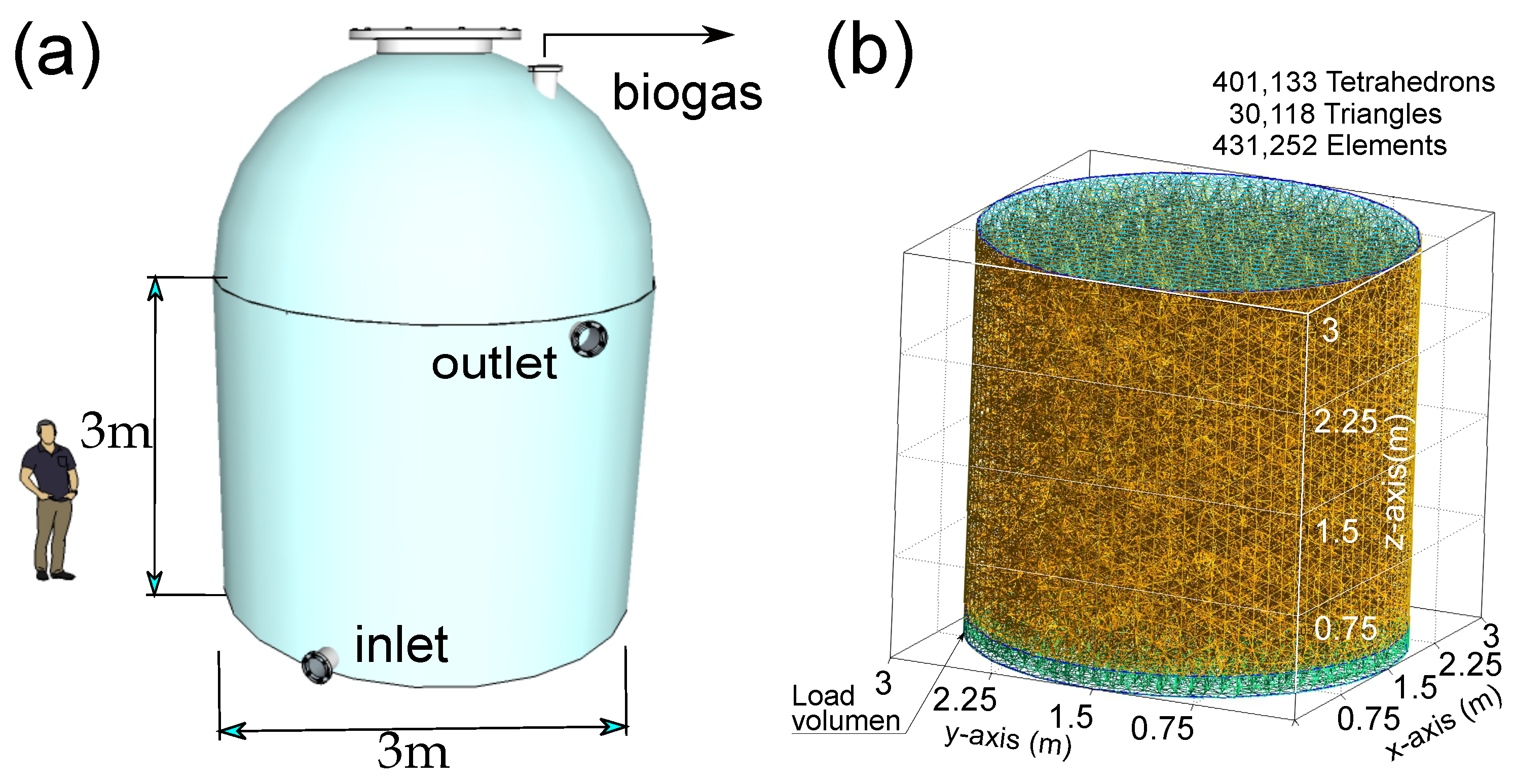
2.5. Case Study
FreeFem++ Code
- 1.
- Definitions of parameters, boundaries and finite element spaces.
- 2.
- Description of macros and functions.
- 3.
- Problem definition.
- 4.
- Loading the loop and calculation of different processes.
- 5.
- Saving the results for manipulation in the post-processes
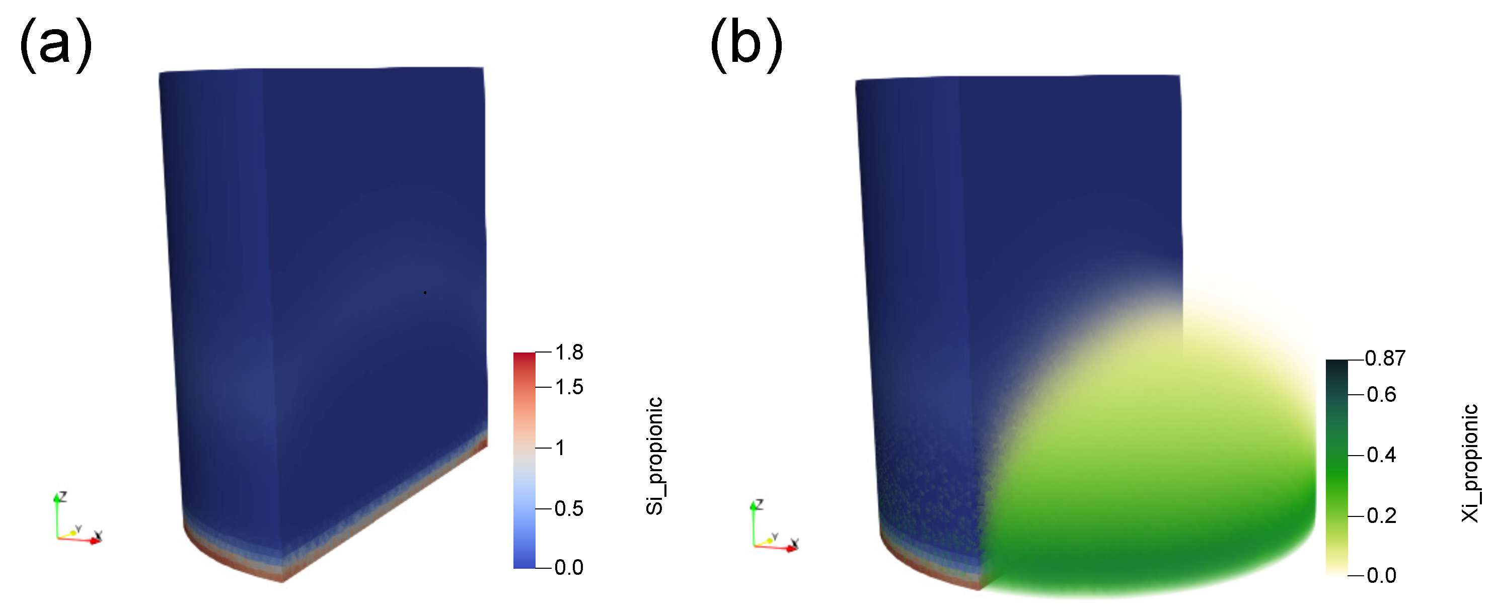
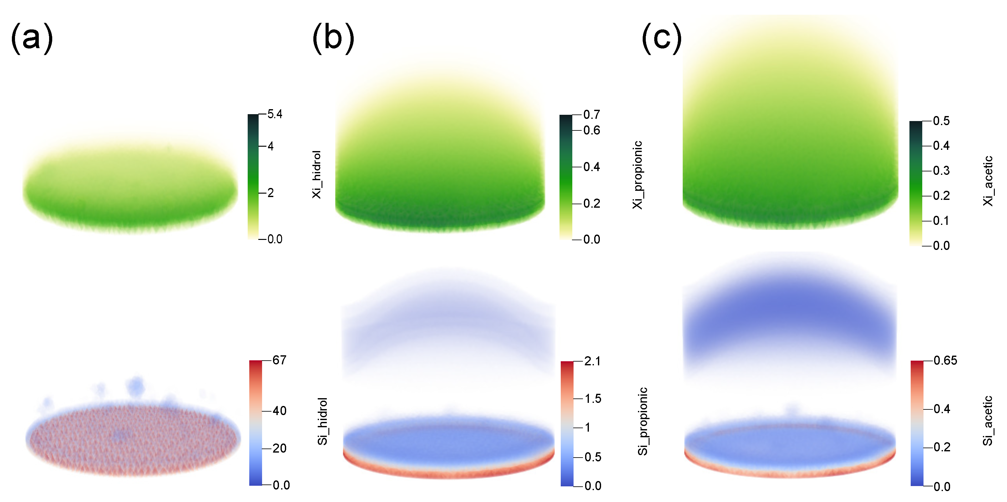
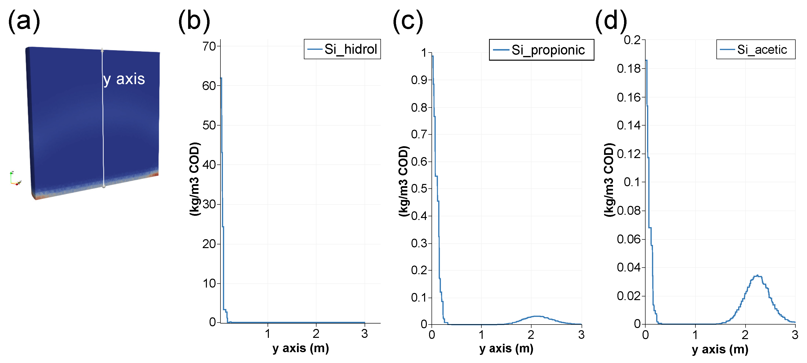
3. Results and Discussion
4. Conclusions
Author Contributions
Funding
Data Availability Statement
Conflicts of Interest
Nomenclature
| Stoichiometric parameters | |
| ; | |
| (d−1) | Specific growth rate |
| (d−1) | Maximum specific growth rate |
| ∇ | ; |
| viscosity of the fluid | |
| represent both the concentration of substrates and cells (kg·m−3) | |
| f | source function. Reactive term |
| (kg m−3) | Saturation constant of the substrate |
| Cell decay rate | |
| Monod substrate saturation constant | |
| (d−1) | Cell decay rate |
| (kg COD m−3) | Substrate concentration |
| (kg COD m−3) | Cells concentration |
| Substrate yield coefficient | |
| Diffusion coefficient | |
| Maximum specific growth rate | |
| velocity vector | |
| F | external force applied to the fluid |
| p | pressure |
| Boundary condition for the substrate | |
| Boundary condition for the microorganism |
Appendix A. FreeFem++ Code
References
- States, N.; Stone, E.; Cole, R. Creating Meaningful Learning Opportunities through Incorporating Local Research into Chemistry Classroom Activities. Educ. Sci. 2023, 13, 192. [Google Scholar] [CrossRef]
- Camilleri, M.A.; Camilleri, A.C. Digital Learning Resources and Ubiquitous Technologies in Education. Technol. Knowl. Learn. 2017, 22, 65–82. [Google Scholar] [CrossRef]
- Liu, D.; Valdiviezo-Díaz, P.; Riofrio, G.; Sun, Y.M.; Barba, R. Integration of Virtual Labs into Science E-learning. Procedia Comput. Sci. 2015, 75, 95–102. [Google Scholar] [CrossRef] [Green Version]
- Watts, J.; Crippen, K.J.; Payne, C.; Imperial, L.; Veige, M. The varied experience of undergraduate students during the transition to mandatory online chem lab during the initial lockdown of the COVID-19 pandemic. Discip. Interdiscip. Sci. Educ. Res. 2022, 4, 14. [Google Scholar] [CrossRef]
- Appels, L.; Lauwers, J.; Degrève, J.; Helsen, L.; Lievens, B.; Willems, K.; Van Impe, J.; Dewil, R. Anaerobic digestion in global bio-energy production: Potential and research challenges. Renew. Sustain. Energy Rev. 2011, 15, 4295–4301. [Google Scholar] [CrossRef]
- Guzmán, J.L.; Joseph, B. Web-Based Virtual Lab for Learning Design, Operation, Control, and Optimization of an Anaerobic Digestion Process. J. Sci. Educ. Technol. 2021, 30, 319–330. [Google Scholar] [CrossRef]
- Husain, A. Mathematical models of the kinetics of anaerobic digestion—A selected review. Biomass Bioenergy 1998, 14, 561–571. [Google Scholar] [CrossRef]
- Wade, M.J. Not Just Numbers: Mathematical Modelling and Its Contribution to Anaerobic Digestion Processes. Processes 2020, 8, 888. [Google Scholar] [CrossRef]
- Batstone, D.J.; Puyol, D.; Flores-Alsina, X.; Rodríguez, J. Mathematical modelling of anaerobic digestion processes: Applications and future needs. Rev. Environ. Sci. Bio/Technol. 2015, 14, 595–613. [Google Scholar] [CrossRef]
- Borisov, M.; Dimitrova, N.; Simeonov, I. Mathematical Modelling of Anaerobic Digestion with Hydrogen and Methane Production. IFAC PapersOnLine 2016, 49, 231–238. [Google Scholar] [CrossRef]
- Batstone, D.; Keller, J.; Angelidaki, I.; Kalyuzhnyi, S.; Pavlostathis, S.; Rozzi, A.; Sanders, W.; Siegrist, H.; Vavilin, V. The IWA Anaerobic Digestion Model No 1 (ADM1). Water Sci. Technol. 2002, 45, 65–73. [Google Scholar] [CrossRef] [PubMed]
- Kleerebezem. Critical analysis of some concepts proposed in ADM1. Water Sci. Technol. 2006, 54, 51–57. [Google Scholar] [CrossRef] [PubMed] [Green Version]
- Li, L.; Wang, K.; Zhao, Q.; Gao, Q.; Zhou, H.; Jiang, J.; Mei, W. A critical review of experimental and CFD techniques to characterize the mixing performance of anaerobic digesters for biogas production. Rev. Environ. Sci. Bio/Technol. 2022, 21, 665–689. [Google Scholar] [CrossRef]
- Hoff, C.; Aurandt, J.; O’Toole, M.; Davis, G. Motivating Student Learning Using Biofuel-Based Activities. In Proceedings of the 2013 ASEE Annual Conference & Exposition (Online), Atlanta, GA, USA, 22–26 June 2020; Available online: https://peer.asee.org/19019 (accessed on 24 January 2023).
- Nanou, P.; Kuchta, D.I.K. Knowledge Transfer Networks in the Field of Biological Waste Treatment: Current Status; Literature Review; Hamburg University of Technology: Hamburg, Germany, 2015. [Google Scholar]
- Sadino-Riquelme, C.; Hayes, R.E.; Jeison, D.; Donoso-Bravo, A. Computational fluid dynamic (CFD) modelling in anaerobic digestion: General application and recent advances. Crit. Rev. Environ. Sci. Technol. 2018, 48, 39–76. [Google Scholar] [CrossRef]
- Song, L.; Li, P.W.; Gu, Y.; Fan, C.M. Generalized finite difference method for solving stationary 2D and 3D Stokes equations with a mixed boundary condition. Comput. Math. Appl. 2020, 80, 1726–1743. [Google Scholar] [CrossRef]
- Ukai, S. A solution formula for the Stokes equation in Rn+. Commun. Pur. Appl. Math. 1987, 40, 611–621. [Google Scholar] [CrossRef] [Green Version]
- Parshotam, A.; Mcnabb, A.; Wake, G. Comparison Theorems for Coupled Reaction-Diffusion Equations in Chemical Reactor Analysis. J. Math. Anal. Appl. 1993, 178, 196–220. [Google Scholar] [CrossRef] [Green Version]
- Muloiwa, M.; Nyende-Byakika, S.; Dinka, M. Comparison of unstructured kinetic bacterial growth models. S. Afr. J. Chem. Eng. 2020, 33, 141–150. [Google Scholar] [CrossRef]
- Monod, J. The Growth of Bacterial Cultures. Annu. Rev. Microbiol. 1949, 3, 371–394. [Google Scholar] [CrossRef] [Green Version]


| Process | |||||||
|---|---|---|---|---|---|---|---|
| d−1 | m2·d−1 | kg· m−3 | kg· m−3 | d−1 | kg· m−3 | kg · kg−1 | |
| 1 | 2.85 | 100 | 0.05 | 0.9 | 0.05 | 10.76 | |
| 2 | 1.8 | - | 0.05 | 0.04 | 1.145 | 11.29 | |
| 3 | 3.9 | - | 0.05 | 0.037 | 0.93 | 18.18 |
Disclaimer/Publisher’s Note: The statements, opinions and data contained in all publications are solely those of the individual author(s) and contributor(s) and not of MDPI and/or the editor(s). MDPI and/or the editor(s) disclaim responsibility for any injury to people or property resulting from any ideas, methods, instructions or products referred to in the content. |
© 2023 by the authors. Licensee MDPI, Basel, Switzerland. This article is an open access article distributed under the terms and conditions of the Creative Commons Attribution (CC BY) license (https://creativecommons.org/licenses/by/4.0/).
Share and Cite
Brito-Espino, S.; García-Ramírez, T.; Leon-Zerpa, F.; Mendieta-Pino, C.; Santana, J.J.; Ramos-Martín, A. E-Learning Proposal for 3D Modeling and Numerical Simulation with FreeFem++ for the Study of the Discontinuous Dynamics of Biological and Anaerobic Digesters. Water 2023, 15, 1181. https://doi.org/10.3390/w15061181
Brito-Espino S, García-Ramírez T, Leon-Zerpa F, Mendieta-Pino C, Santana JJ, Ramos-Martín A. E-Learning Proposal for 3D Modeling and Numerical Simulation with FreeFem++ for the Study of the Discontinuous Dynamics of Biological and Anaerobic Digesters. Water. 2023; 15(6):1181. https://doi.org/10.3390/w15061181
Chicago/Turabian StyleBrito-Espino, Saulo, Tania García-Ramírez, Federico Leon-Zerpa, Carlos Mendieta-Pino, Juan J. Santana, and Alejandro Ramos-Martín. 2023. "E-Learning Proposal for 3D Modeling and Numerical Simulation with FreeFem++ for the Study of the Discontinuous Dynamics of Biological and Anaerobic Digesters" Water 15, no. 6: 1181. https://doi.org/10.3390/w15061181