
Leakage Detection in Water Distribution Networks Based on Multi-Feature Extraction from High-Frequency Pressure Data

1
School of Environmental Science and Engineering, Tianjin University, Tianjin 300350, China
2
School of Earth and Space Sciences, University of Science and Technology of China, Hefei 230026, China
*
Author to whom correspondence should be addressed.
Water 2023, 15(6), 1187; https://doi.org/10.3390/w15061187
Submission received: 21 February 2023
/
Revised: 11 March 2023
/
Accepted: 17 March 2023
/
Published: 19 March 2023
(This article belongs to the Special Issue Green and Low Carbon Development of Water Treatment Technology)
Abstract
:Leakage detection is an important task to ensure the operational safety of water distribution networks. Leakage characteristic extraction based on high-frequency data has been widely used for leakage detection in experimental networks. However, the accuracy of single-feature-based methods is limited by the interference of background pressure fluctuations in networks. In addition, the setting of leakage diagnosis thresholds has been insufficiently studied, but influences leakage detection performance greatly. Hence, a new method of leakage detection is proposed based on multi-feature extraction. The multi-features of leakage are composed of instantaneous characteristics (ICs) and trend characteristics (TCs), which constitute comprehensive leakage information. The levels of the instantaneous and trend pressure drops in background pressure fluctuations in network environments are quantified for the setting of leakage diagnosis thresholds. In addition, ICs and TCs are used for leakage degree prediction. The proposed method was applied to an experimental network. Compared with the single-feature-based method and the cumulative sum (CUSUM) method, the proposed method achieved increases of 6.01% and 13.66% in F-Scores, respectively, and showed better adaptability to background pressure fluctuations in complex network environments.
1. Introduction
Water, especially fresh water, is a scarce resource for human existence and development. However, for various reasons, such as pipeline aging, inappropriate design and operation, and lack of maintenance, pipelines in water distribution networks (WDNs) often encounter leakage, blockage, corrosion, and other failures, resulting in a large amount of water loss [1,2]. It has been estimated that the volume of non-revenue water (NRW) is 126 billion m3 per year, which causes a financial cost of USD 39 billion per year [3]. Leakage is one of the most common and harmful failures, as it causes huge water waste and poses big challenges to the daily operations and maintenance of systems. The World Bank estimated that the annual leakage volume in urban water distribution networks was close to 50 billion m3 worldwide, which accounted for more than 15% of the total annual water supply volume [4]. Leakage events also cause socioeconomic losses due to disruption to production processes, damage to property, and increased energy costs for pumping and supplying water [2,5]. In addition, leakage may lead to the intrusion of pollutants into the pipeline, resulting in water-quality deterioration [6]. Therefore, leakage detection is of great significance for saving water resources, reducing economic loss, and ensuring the operational safety of WDNs.
Leakage detection methods based on high-frequency data analysis have been widely studied because of their potential for complete preservation and the rapid extraction of leakage information [2]. At present, leakage detection methods based on high-frequency data can be divided into active leakage detection methods and passive leakage detection methods [7,8,9,10]. Active leakage detection methods utilize actively generated transient flow excitation signals to detect existing leaks in a pipeline [11,12]. After the generation and measurement of transient waves, leakage events can be detected based on transient reflection, transient damping, transient frequency response, inverse transient analysis, or signal processing [1,2]. Further, advanced data analysis methods, such as forward–backward transient analysis and the Dempster–Shafer evidence framework, have also been proved to achieve good performance in leakage detection [12,13].
Passive leakage detection methods use real-time monitoring data to capture transient flow signals which are generated by new leakages in networks [14,15]. Compared with active leakage detection methods, passive leakage detection methods do not need excitation signal generation, and thus have broader application prospects for actual complex networks. When a leakage event occurs in a WDN, it generates a negative pressure wave in the network, which is shown as a singularity in a high-frequency signal, whether it is a pressure signal or an acoustic signal [16]. Therefore, different methods can be used to extract the singularity in a high-frequency signal as the leakage characteristic. Due to the characteristics of multi-scale analysis in both the time and frequency domains, the wavelet transform (WT) is very suitable for singularity identification and has been widely applied for leakage detection [17,18]. The wavelet transform coefficients obtained by the continuous wavelet transform (CWT) and the detail coefficients obtained by the discrete wavelet transform (DWT) could both be used as leakage characteristics for leakage detection [19,20,21]. On this basis, methods of leakage characteristic extraction were optimized to increase leakage information contained in leakage characteristics. The optimal selection of the mother wavelet could significantly improve the quality of leakage characteristics [22,23]. In addition, the improvement of the wavelet transform also proved to be beneficial for the extraction of leakage characteristics [24,25]. The above methods can effectively detect a singularity in a signal, but sometimes it is hard to distinguish whether it is caused by leakage or background noise.
Statistics-based methods are another set of methods for leakage detection because of their sensitivity to the trend pressure drops in networks. The cumulative sum (CUSUM) method was successfully used to diagnose abrupt pressure changes and detect leakage events [26]. The improved method based on cumulative integral, floor function, and curvature achieved the detection of small leakage events and a reduction in false alarm rates [27]. Moreover, water balance analysis and the theory of DMA based on flow monitoring and valve operations have also been applied to leakage detection and show wide practical application prospects [5]. These methods can avoid noise interference but may also readily misdetect background pressure fluctuations caused by variations in water consumption as leakage events. In addition to the optimization of leakage characteristics, the emergence of machine learning and deep learning models has also provided new methods for the diagnosis of leakage characteristics. Different leakage characteristics and classification models have been used to obtain high leakage detection accuracies [28,29,30,31]. These models can adaptively achieve leakage diagnosis based on training data sets, thus avoiding the difficulty of threshold setting. Nevertheless, the interpretability of machine learning models needs to be improved, and these models can only adapt to different network environments by updating the training data sets, which limits their further practical applications.
The above methods mainly focus on a single leakage characteristic based on the singularity of a negative pressure wave or statistical fluctuations. However, when a leakage event occurs in a WDN, the characteristics of a negative pressure wave and statistic fluctuations are contained in the high-frequency data, which means that leakage information extracted by single-feature-based methods is incomplete and limits leakage detection accuracy under the interference of noise and variations in water consumption [15]. To improve leakage detection performance, it is necessary to extract multiple characteristics and obtain comprehensive leakage information. In addition, it is important to set appropriate thresholds, as these determine the performance of leakage diagnosis. However, this is difficult under circumstances of background pressure fluctuations in WDNs [32]. Although there are several articles describing the setting of thresholds [19,33,34], quantitative studies of the levels of background pressure fluctuations in WDNs are lacking, and the analysis of thresholds is often ignored, which limits the adaptability of methods to actual WDNs. Hence, the levels of background pressure fluctuations in WDNs, which could provide references for threshold setting in leakage diagnosis, should be evaluated.
Therefore, a leakage detection method based on multi-feature extraction is proposed in this paper. The instantaneous characteristics and the trend characteristics of leakage events were extracted from high-frequency pressure data for a WDN which could provide comprehensive leakage information and enable the interference of noise and variations in water consumption to be overcome. In addition, the setting of thresholds for leakage diagnosis was analyzed based on the quantification of background pressure fluctuations in the network environment, which could guide the reasonable setting of thresholds. Then, the optimal thresholds were determined to diagnose leakage events. Finally, the leakage degrees of the detected leakage events were predicted based on leakage characteristics. The proposed method was verified on an experimental network and also compared with the single-feature-based method and the CUSUM method and showed the best leakage detection performance.
2. Methodology
2.1. Overview of the Proposed Method
The framework of the leakage detection method based on multi-feature extraction proposed in this paper is shown in Figure 1; it mainly consists of four parts:
- (1)
- Data Preprocessing
The original high-frequency pressure time series s00 was processed by the Butterworth band-stop filter for the removal of measurement noise. The filtered time series s0 was obtained from time series s00, which was ready for the extraction of leakage characteristics. The multi-features of leakage are composed of instantaneous characteristics (ICs) and trend characteristics (TCs). IC refers to an instantaneous drop and the instantaneous increase in pressure caused by the negative pressure wave generated by a leakage [10]. TC means the increased flow caused by a leakage event which leads to a certain degree of trend pressure drop in a network.
- (2)
- Instantaneous Characteristic Diagnosis (IC Diagnosis)
The continuous wavelet transform (CWT) was performed on time series s0 to extract the ICs and obtain the IC time series s1. Then, an appropriate threshold for ICs (thric) was analyzed and set according to the instantaneous pressure drop levels of the background pressure fluctuations in the network environment. When there was a maximum point p in time series s1 whose IC value exceeded thric, a probable leakage event at point p was diagnosed.
- (3)
- Trend Characteristic Diagnosis (TC Diagnosis)
For the point p with a probable leakage event, the trend time series s2,p was obtained with a smoothing process from the time series s0. CWT was performed on time series s2,p to extract the TCs and obtain the TC time series s3,p. An appropriate threshold for TCs (thrtc) was analyzed and set according to the trend pressure drop levels of the background pressure fluctuations in the network environment. When the maximum in the time series s3,p exceeded thrtc, it was diagnosed that a leakage event had occurred at point p, and the leakage alarm was triggered for further analysis.
- (4)
- Leakage Degree Prediction
ICs and TCs of leakage events are both related to leakage degrees. Pearson’s correlation coefficient (PCC) was used to evaluate the correlation between leakage flow and two leakage characteristics and select a suitable leakage characteristic as the indicator for leakage degree prediction. Then, the relationship between the selected leakage characteristic and leakage flow was determined through linear fitting. Leakage flow of newly detected leakage events could be predicted with leakage characteristic values. Based on leakage flow classification, leakage degree was predicted as severe leakage or small leakage.
2.2. Data Preprocessing
The raw data collected by a high-frequency pressure sensor in a network often contains plenty of noise due to electromagnetic interference, the opening and closing of valves, the vibration of the devices, and other factors [35], resulting in leakage signals being hidden and difficult to identify. Therefore, noise filtering is necessary for leakage signal analysis. Considering that Butterworth filters are maximally flat in their pass-bands, they are suitable for smoothing movement data [35,36]. Therefore, the original high-frequency pressure time series s00 was filtered by the Butterworth band-stop filter in this paper. The Butterworth band-stop filter uses the Fourier transform to convert the signal from the time domain to the frequency domain. According to the frequency characteristics of the signal, the noise signal is removed, and the effective signal is retained. The transfer function of the Butterworth band-stop filter is given in Equation (1):
where n is the order of the filter, f is the frequency, and fc is the cut-off frequency. The pressure fluctuation of the high-frequency signal becomes clear after filtering, as shown by time series s0 in Figure 1.
2.3. IC Diagnosis
2.3.1. IC Extraction
CWT was performed on time series s0 to obtain the IC time series s1. The formula of CWT is shown in Equation (2):
where Wf (α,τ) is called the wavelet transform coefficient, which is the inner product of the mother wavelet and the time series in scale α and displacement τ, reflecting the similarity between the time series and the mother wavelet at the scale α and displacement τ. Since the wavelet has the characteristic of rapid decay, it reflects the properties of the time series near the displacement τ.
For the leakage signal in the high-frequency pressure time series, the shape of the instantaneous pressure drop caused by the negative pressure wave is similar to the Haar wavelet, and the discontinuity characteristic of the Haar wavelet is excellent for the detection of breakpoints in the signal [29,33]. Therefore, the Haar wavelet was chosen as the mother wavelet when CWT was performed on time series s0. The wavelet transform coefficient of each point obtained by CWT means the IC value at the point and reflects the instantaneous pressure drop amplitude at the point in time series s0.
2.3.2. IC Threshold Analysis
The wavelet transform coefficient in time series s1 was calculated based on fluctuations in pressure over a very short period. On the same time scale, both leakage events and the background pressure fluctuations caused by noise in the network may produce a similar shape of instantaneous pressure drop. Therefore, it is necessary to set an appropriate threshold for ICs to distinguish background pressure fluctuations and leakage events effectively. The leakage-free time series data set was used to evaluate the instantaneous pressure drop levels of the background pressure fluctuations and determine the threshold for ICs. The threshold for ICs was calculated as follows:
where thric is the threshold for ICs, meanic and σic are the mean and the standard deviation of the leakage-free time series data set, and αic is the threshold coefficient for ICs, which is used to adjust the strictness of the diagnosis of ICs. The IC value of the maximum point p in time series s1 was compared with thric. When the IC value of point p exceeded thric, this meant that the instantaneous pressure drop at point p was most likely not caused by the background pressure fluctuations in the network. Hence, it was diagnosed that there was a probable leakage event at point p.
2.4. TC Diagnosis
2.4.1. TC Extraction
For each point p whose IC value exceeded thric in Section 2.3, the pressure data of the length l before and after the point p in time series s0 was taken to obtain the time series s0,p,before and the time series s0,p,after, respectively, as shown in Equations (6) and (7):
After the smoothing process, s2,p,before and s2,p,after were obtained from s0,p,before and s0,p,after and concatenated into the trend time series s2,p, which reflected the average pressure level before and after point p. The sliding time window theory was used to calculate the average pressure value of each point in the smoothing process [31]. The formulas of the smoothing process are as follows:
where cl is the window length, which is used to adjust the smoothness of the original signal. Time series s2,p obtained by the smoothing process can more clearly show the trend change characteristics of pressure. The TC time series s3,p was obtained by performing CWT on s2,p. The Haar wavelet was also chosen as the mother wavelet when performing CWT on time series s2,p. The maximum in the time series s3,p means the TC value at point p and reflects the trend pressure drop amplitude at point p in time series s0.
2.4.2. TC Threshold Analysis
Both leakage events and variations in water consumption may lead to trend pressure drops. Therefore, as in Section 2.3, the leakage-free time series data set was used to evaluate the trend pressure drop levels of the background pressure fluctuations, and the appropriate threshold for TCs was set to distinguish background pressure fluctuations and leakage events. The calculation of the threshold for TCs was as follows:
where thrtc is the threshold for TCs, meantc and σtc are the mean and the standard deviation of the leakage-free time series data set, and αtc is the threshold coefficient for TCs, which is used to adjust the strictness of the diagnosis of TCs. When the maximum in the time series s3,p exceeds thrtc, this means that the trend pressure drop amplitude at point p exceeds the normal range of the background pressure fluctuations in the network. Then, it is diagnosed that a new leakage event occurs at point p.
To sum up, the multi-features of leakage were extracted first via the proposed method, which includes ICs and TCs. Then, two thresholds of thric and thrtc were set based on leakage-free time series to comprehensively diagnose whether there existed leakage events in the network. In this paper, IC and TC were diagnosed in series rather than in parallel, the purpose of this being to reduce the computational cost of the process of TC extraction.
2.5. Leakage Degree Prediction
The two leakage characteristics of IC and TC extracted in Section 2.3 and Section 2.4, respectively, are related to leakage degree. In this paper, leakage flow was used to measure leakage degree. For different network environments, Pearson’s correlation coefficient (PCC) was used to reflect the linear correlation between the two leakage characteristics and leakage flow and select a suitable leakage characteristic as the indicator to predict leakage degree. The calculation of PCC is shown in Equation (13):
where X and Y are the two variables. PCC is in the range of −1 to 1. When PCC exceeds 0.8, it can be considered that X and Y are highly positively correlated. Then, the selected leakage characteristic and leakage flow were linearly fitted for leakage degree prediction. For a newly diagnosed leakage event, leakage flow is predicted with the extracted leakage characteristic value. Based on the predicted leakage flow, the detected leakage event is classified as severe leakage or small leakage and the predicted leakage degree is obtained, which provides a reference for the leakage repair response level of the water company.
3. Results and Discussion
3.1. Experimental Network Setup
In this paper, a small experimental network with two loops was built to collect experimental data, as shown in Figure 2. The experimental network covers an area of about 100 m2, and the total length of the pipeline is 52 m. The network includes a tank, a water pump, 3 pipes of 100 mm diameter, 11 pipes of 50 mm diameter, and 1 pipe of 25 mm diameter. There are three monitoring points in the network, and each monitoring point is equipped with a high-frequency pressure sensor and an ultrasonic flowmeter. The sampling frequency of the pressure sensor is 10,000 Hz, and the sampling frequency of the flowmeter is 1 Hz. There are seven leakage simulators in the network to simulate leakage events. The opening status and opening range of each leakage simulator are controlled by a valve. The diameter of the leakage simulator A6 is 32 mm, and the diameters of the other leakage simulators are 15 mm. The water in the tank flows into the network after being pressurized by the pump and finally flows back into the tank through valves X1 and X2.
In this paper, several sets of leakage experiments under different working conditions were designed and carried out. The overall pressure level of the network was in the range of 5–30 m, which could be adjusted by changing the operating parameters of the pump. The total flow level of the network was in the range of 2.5–23 L/s, which could be controlled by valves X1 and X2. The flow rate of leakage events was in the range of 0.04–9.5 L/s, which was controlled by changing the opening range of the valve at each leakage simulator. In addition, variations in water consumption in the actual network were imitated by slowly and randomly adjusting valves at the leakage simulators. Finally, time series without and with the imitation of variations in water consumption were collected to form the steady-state time series data set and the water-consumption time series data set, respectively.
Each time series data set included high-frequency pressure data for multiple leakage events and leakage-free events. Each event corresponded to a group of time series, including three high-frequency pressure time series collected at three monitoring points in the same period. The length of each time series was 4 s, and the sampling frequency was 10,000 Hz. The steady-state time series data set contained 352 groups of leakage time series and 2816 groups of leakage-free time series, while the water-consumption time series data set contained 78 groups of leakage time series and 624 groups of leakage-free time series.
3.2. Performance Indicators and Method Parameters
3.2.1. Performance Indicators
For each event in the two time series data sets, the label was unique. The label of a leakage event was “L”, and the label of a leakage-free event was “NL”. When it was detected that a leakage event occurred in at least one time series in the group of time series corresponding to the same event, the output of the event was “L”. Otherwise, the output of the event was “NL”. Since the labels for each group of time series were only “L” or “NL”, the leakage detection problem could be regarded as a binary classification problem. Thus, a confusion matrix (see Table 1) can be used to describe the performance of the proposed leakage detection method [37].
The confusion matrix can be used to calculate Precision, Recall, F-Score, False Alarm Rate (FAR), and Missing Alarm Rate (MAR) to evaluate the performance of the method, as shown in Equations (14) to (18):
Precision measures the reliability of the output of the method. Recall measures the ability of the method to detect leakage events. F-Score is the harmonic average of Precision and Recall, and β is used to adjust the weights of Precision and Recall in different tasks. When Precision is more important, β can take a value greater than 1. Considering that the water company hoped to detect as many leakage events as possible in the actual leakage detection work, β was taken as 2 in this paper to increase the weight of Recall. Precision, Recall, and F-Score were used to select the appropriate αic and αtc, while FAR and MAR were used to describe the leakage detection results for the time series data sets.
3.2.2. Parameters for Multi-Feature Extraction
An appropriate scale α in Equation (2) is set to represent IC information in the time dimension. α should be close to the total duration of the ICs of leakage events. The calculation of the total duration of an IC is defined in Figure 3. The instantaneous pressure drop duration, the instantaneous pressure increase duration, and the total duration of IC of leakages in 1065 time series in the steady-state time series data set were determined, as shown in Figure 4. The results show that the instantaneous pressure drop duration of 75.49% leakages was in the range of 500–1500, that the instantaneous pressure increase duration of 71.55% leakage was not more than 1000, and that the total duration of IC of 81.88% leakages was not more than 2500. Therefore, α was taken as 2500 in the extraction of the IC.
l in Equations (6) and (7) was taken as 10,000, and cl in Equation (8) was taken as 2000, which indicated that the pressure value of each time point in the time series s2,p reflected the average pressure level within 0.4 s around the point p and avoided the influence of the noise. When CWT was performed on time series s2,p, the change in α did not significantly affect the detection of TCs due to the elimination of ICs in the time series s2,p. Considering that the pressure fluctuations caused by variations in water consumption might have an impact on the calculation of the average pressure drop levels caused by leakage events, α was taken as 1000 in the extraction of TCs.
3.3. Results for Two Time Series Data Sets
3.3.1. Leakage Detection Results
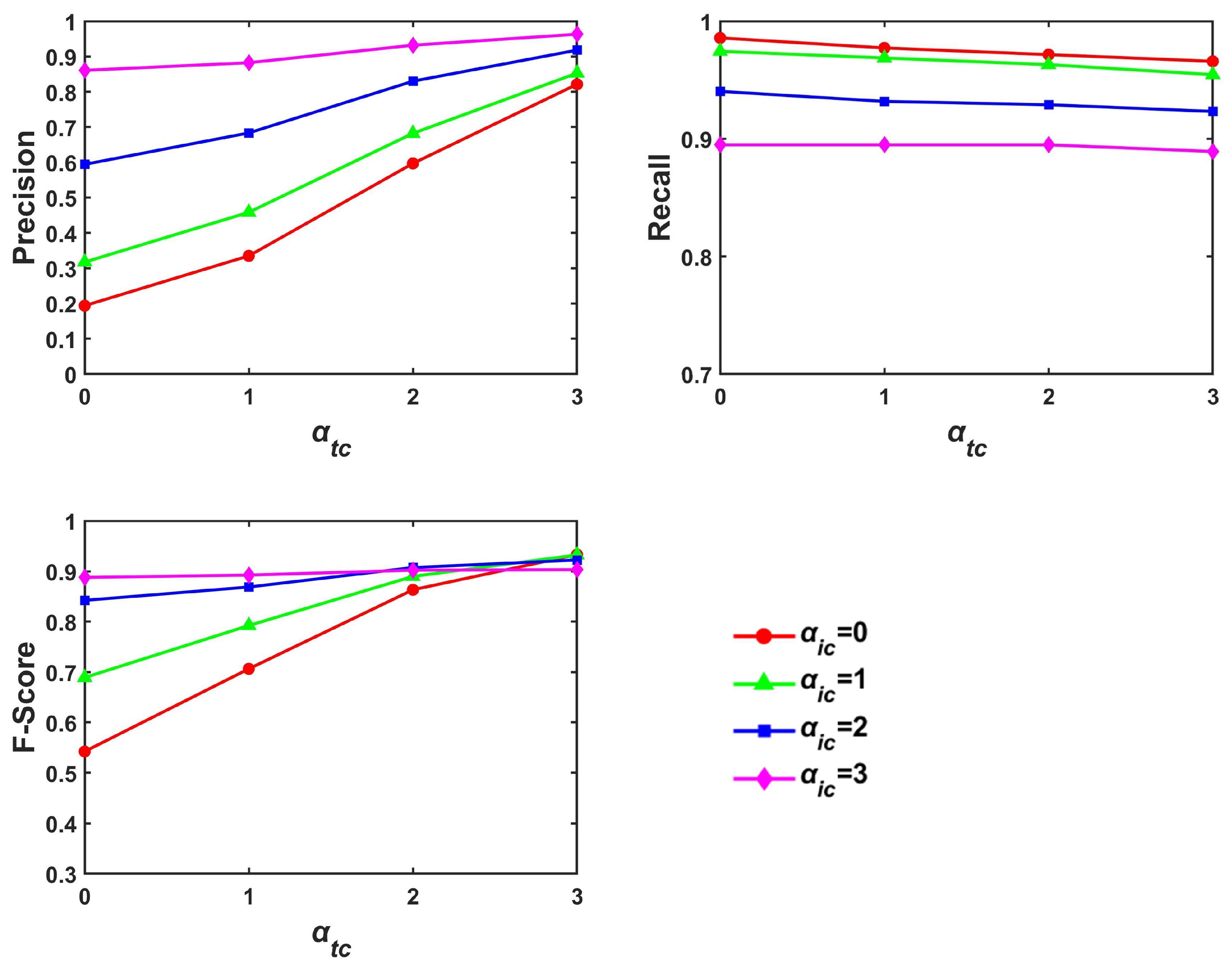
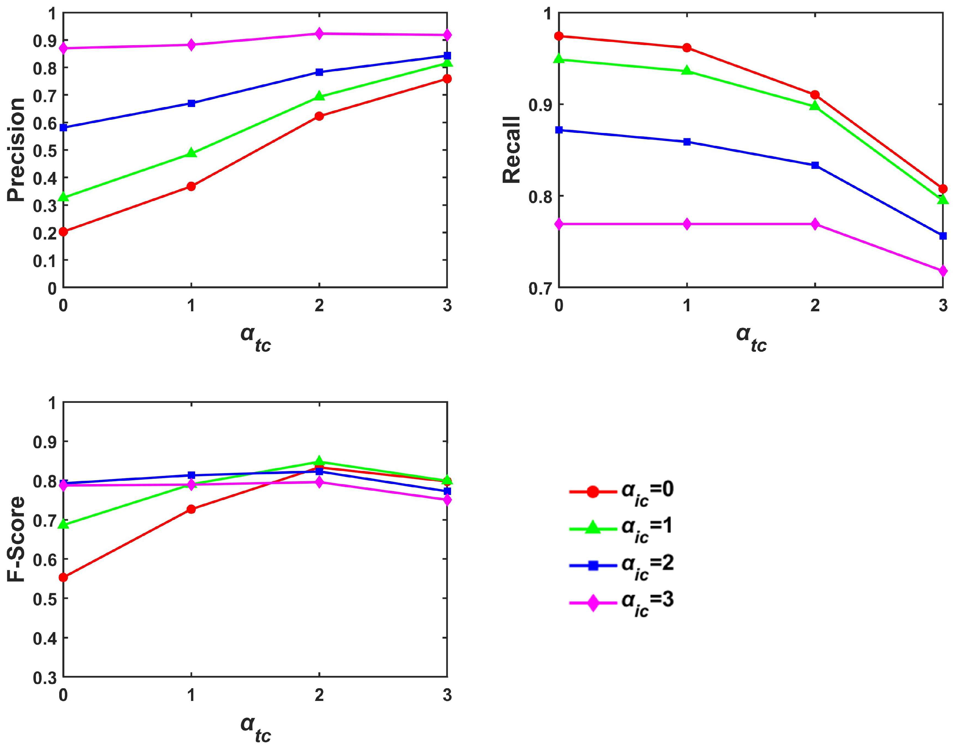
Figure 5 and Figure 6 show the leakage detection performance of the method on the steady-state time series data set and the water-consumption time series data set under different αic and αtc, respectively. With increase in αic and αtc, thric and thrtc increase correspondingly, the diagnostic criteria for ICs and TCs become stricter, and more background pressure fluctuations and small-degree leakage events are not detected as leakage events, resulting in an increase in Precision and a decrease in Recall. Hence, F-Scores were used to balance Precision and Recall and select the appropriate thresholds. Finally, αic and αtc in the steady-state time series data set took 0 and 3 to obtain the maximum F-Score of 93.30%, and αic and αtc in the water-consumption time series data set took 1 and 2 to obtain the maximum F-Score of 84.75%. Compared with the steady-state time series data set, the increase in αic and αtc in the water-consumption time series data set had a more significant impact on Recall but roughly the same impact on Precision, which means that variations in water consumption create huge challenges in the diagnosis of small leakage events.
The leakage detection results for the two time series data sets are shown in Table 2. On the one hand, the proposed method successfully extracted multi-features of leakage information and achieved accuracy and reliability in leakage detection. On the other hand, the existence of variations in water consumption inevitably affected the performance of leakage detection, causing an increase of 2.34% in FAR and an increase of 6.85% in MAR.
3.3.2. Leakage Degree Prediction Results
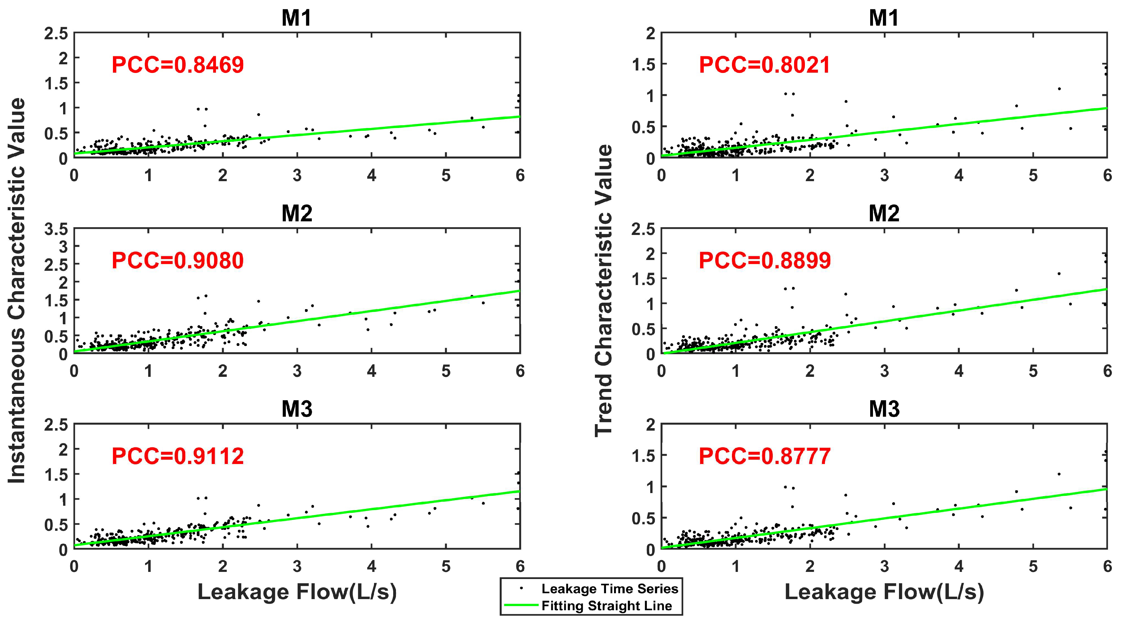
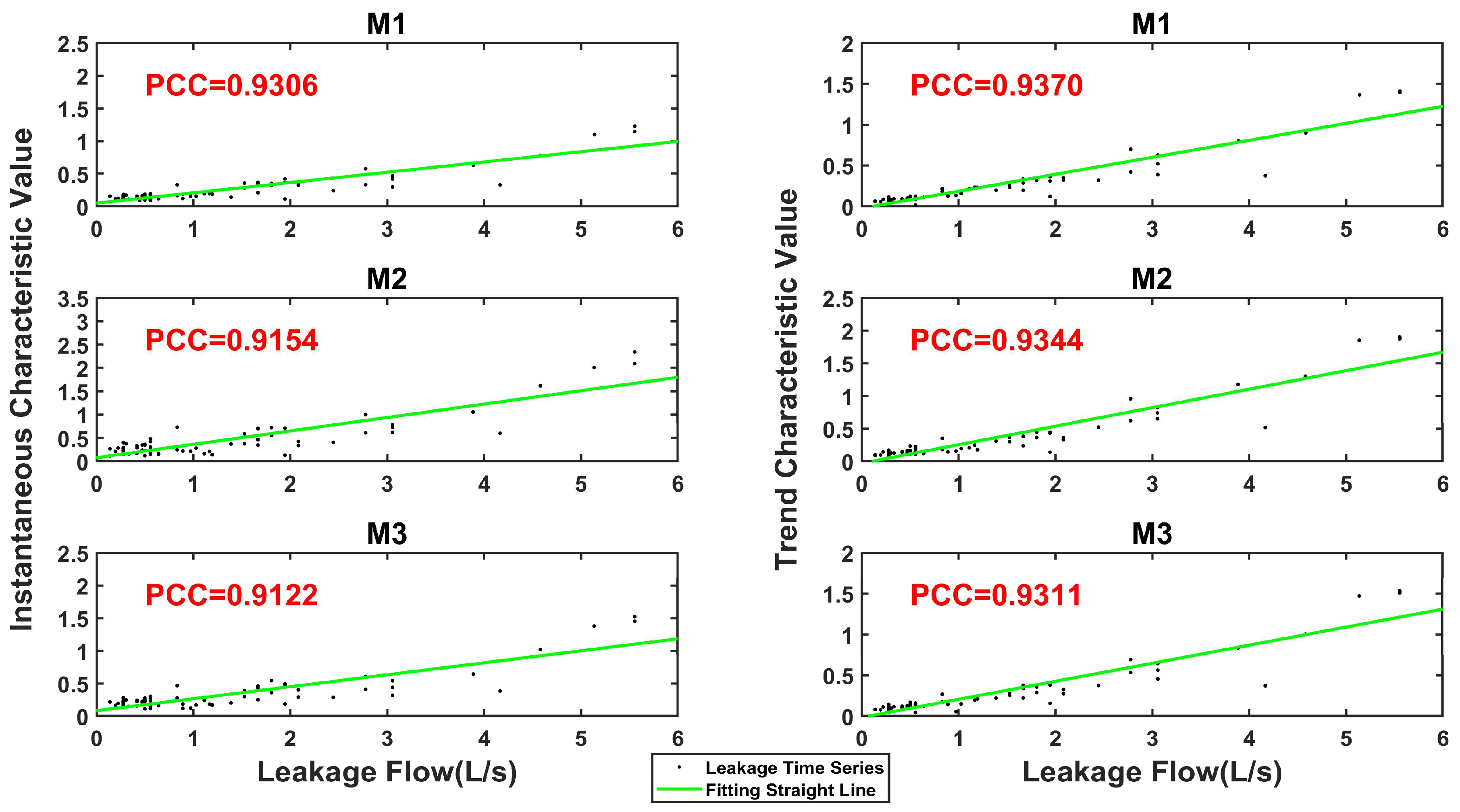
Figure 7 and Figure 8 present the relationships between leakage flow and the two leakage characteristics successfully detected in two time series data sets. For the two time series data sets, PCCs between leakage flow and the two characteristics at three monitoring points were all higher than 0.8, which indicates that the ICs and TCs of leakage events are both highly positively correlated with leakage flow. In the steady-state time series data set, the average PCC between leakage flow and IC at three monitoring points was 0.8887, and the average PCC between leakage flow and TC at three monitoring points was 0.8566. Hence, IC was selected as the indicator for predicting the leakage flow of leakage events in the steady-state time series data set. Different from the steady-state time series data set, the average PCC between leakage flow and ICs at three monitoring points was 0.9194 for the water-consumption time series data set, and the average PCC between leakage flow and TCs at three monitoring points was 0.9342. Hence, TC was selected as the indicator for predicting the leakage flow of leakage events in the water-consumption time series data set.
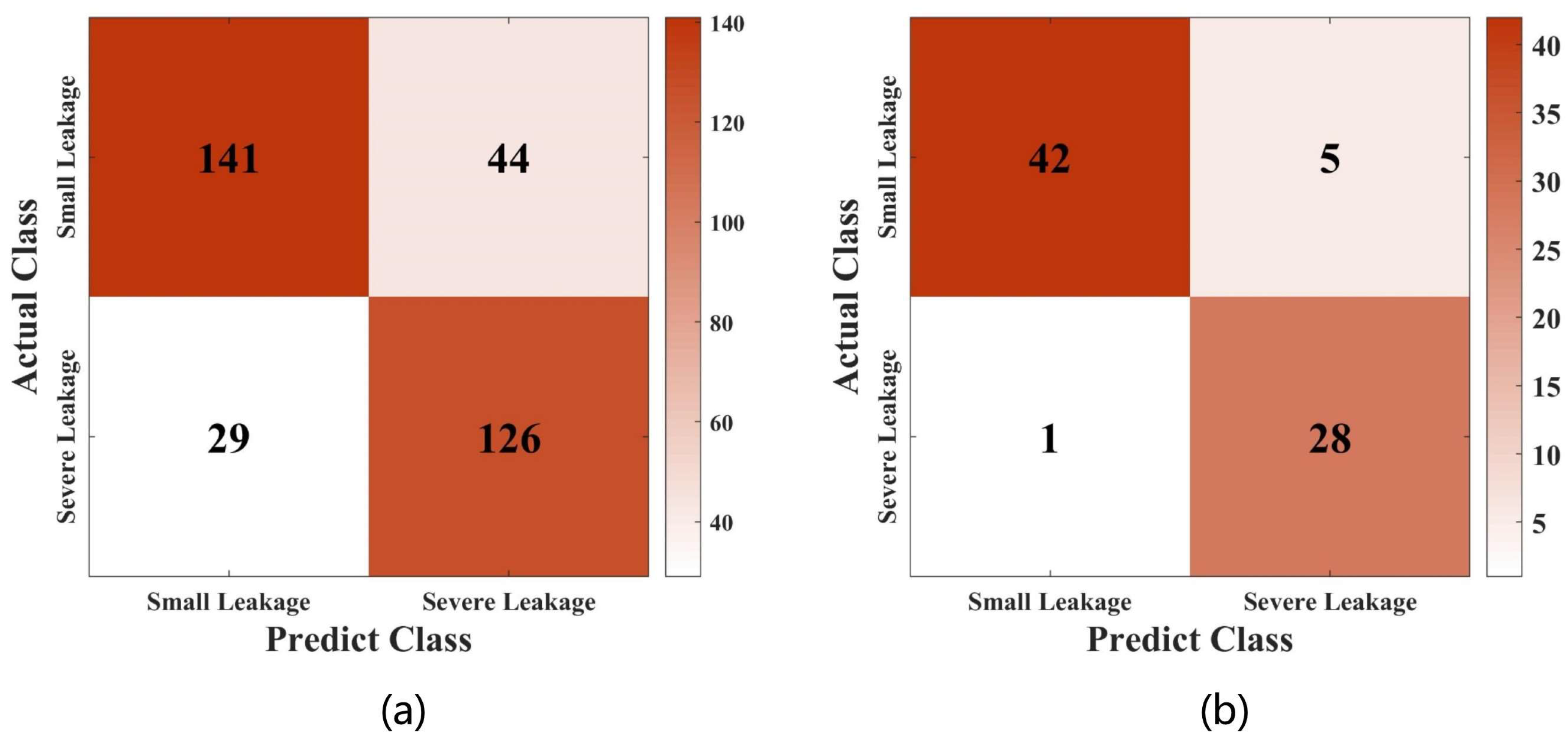
In order to further verify the performance of leakage degree prediction, according to the distribution of leakage flow in two time series data sets in this paper, leakage events were divided into severe leakages (more than 1 L/s) and small leakages (no more than 1 L/s), which kept the number of time series with severe leakages roughly balanced with the number of time series with small leakages. For leakage detection in real WDNs, water companies can set different classification methods for leakage events according to their own needs. The confusion matrix in Figure 9a represents the results for leakage degree prediction for the steady-state time series data set. The results show that the accuracy of leakage degree prediction reached 78.53% for all the successfully detected leakage events. The confusion matrix in Figure 9b shows that the accuracy of leakage degree prediction reached 92.11% for all the successfully detected leakage events in the water-consumption time series data set. The results for leakage degree prediction for the two time series data sets indicate that the two leakage characteristics both contain information on leakage degree and can be used to predict leakage flow. Meanwhile, the existence of variations in water consumption in the network does not interfere with the prediction accuracy for leakage flow. On the contrary, the accuracy of leakage degree prediction for the steady-state time series data set was 13.58% lower than that for the water-consumption time series data set. This result was mainly due to the fact that the number of time series with leakage flow around 1 L/s in the steady-state time series data set was larger than that in the water-consumption time series data set, which can be seen in Figure 7 and Figure 8. The proposed method achieved a high accuracy of leakage degree prediction on both two time series data sets, and thus has good adaptability to different network environments. In actual leakage detection, the water company needs to strike a balance between reducing the waste of water resources and reducing maintenance costs, as it cannot completely avoid false-alarm events. Therefore, leakage degree predicted by the proposed method can accurately reflect the severity of a leakage event and provide a reference for the water company to take a proper response level of leakage repair.
3.4. Discussion
3.4.1. Adaptability Analysis of Threshold Setting
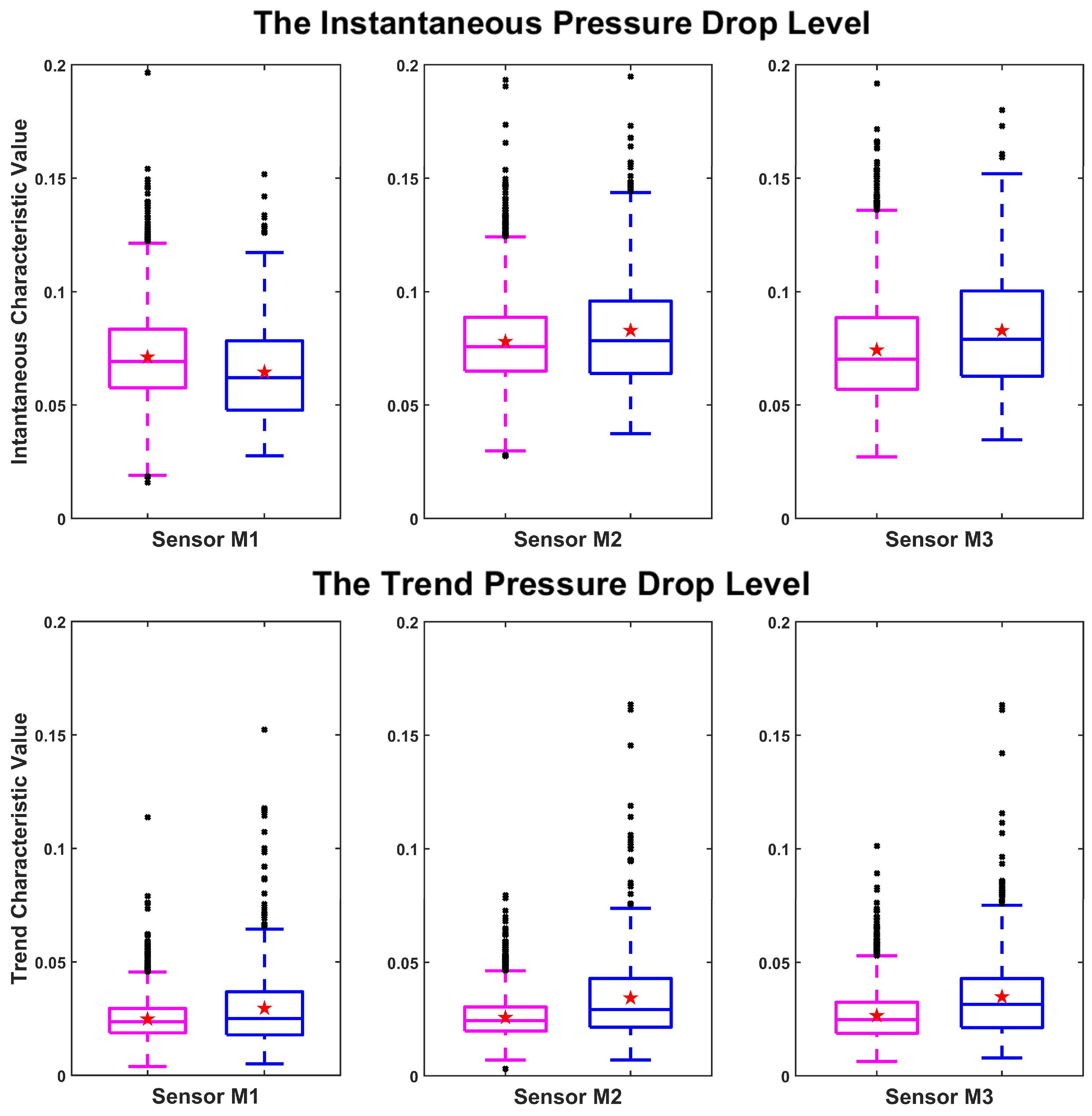
To explore the influence of variations in water consumption on leakage detection, the distributions of two leakage characteristics of leakage-free time series were calculated and these were used to reflect the instantaneous and trend pressure drop levels of background pressure fluctuations in two different network environments. The results are shown in Figure 10, in which the red stars and the middle lines in the boxes represent the means and the medians of the time series data sets, respectively.
The effectiveness of the leakage detection method is based on the significant distribution differences in pressure drop levels between the leakage time series data sets and the leakage-free time series data sets. Therefore, the variations in the pressure drop levels of background pressure fluctuations will affect leakage detection performance. Here, the average pressure drop level is defined as the average of the median and the mean of a time series data set. As shown in Figure 10, with the addition of variations in water consumption, there was a small rise of 2.37% in the instantaneous average pressure drop level of the leakage-free time series, while the trend average pressure drop level of the leakage-free time series rose significantly by 22.92%.
When the average drop level of the leakage-free time series increases, this means a higher coincidence degree of the distribution of leakage characteristics between the leakage time series and the leakage-free time series, such that some small leakage events are undetectable and some background pressure fluctuations are misreported, leading to reductions in leakage detection performance. Therefore, it can be inferred that the existence of variations in water consumption has a slight impact on IC diagnosis but a significant impact on TC diagnosis.
The threshold coefficient represents the strictness of leakage diagnosis. The optimal threshold coefficients of the two time series data sets mentioned in Section 3.3.1 are shown in Table 3. In the steady-state time series data set, αic took the value of 0 and αtc took the value of 3, which meant that the coincidence degree of ICs between the distributions of the leakage time series and the leakage-free time series was much higher than that of TCs in the network environment without variations in water consumption. Hence, αic took the laxest value to decrease MAR and αtc took the strictest value to decrease FAR. With the addition of variations in water consumption, there was a small increase in the coincidence degree of ICs but a significant increase in the coincidence degree of TCs. Therefore, αtc should be reduced to avoid a steep increase in MAR. At this time, αic should be increased to improve the overall performance of leakage detection. As a result, αic took 1 and αtc took 2 in the water-consumption time series data set.
In the above discussion, the adaptability of threshold setting to variations in water consumption has been analyzed, providing an applicable reference for reasonable threshold setting for leakage diagnosis in complex network environments. In actual WDNs, trend pressure drop levels more accurately reflect the characteristics of variations in water consumption than instantaneous pressure drop levels and thus can be used to adjust αic and αtc appropriately and improve adaptability to different network environments. For instance, when there are slight variations in water consumption in a network during the night, a low αic and a high αtc, is suggested, e.g., 0 and 3, and when variations in water consumption become greater during the daytime, a higher αic and a lower αtc are needed.
3.4.2. Comparison of Three Methods for Leakage Detection
To verify the adaptability of the proposed method to variations in water consumption, the single-feature method based on IC and the CUSUM method based on statistics were applied to the two time series data sets and compared with the proposed multi-feature-based method. As in Section 2.3, the same method of threshold determination was used in the two methods to diagnose leakage events. Figure 11 shows the influence of the threshold coefficient on leakage detection performance based on different methods. As the threshold coefficient increased, Precisions all increased significantly and Recalls decreased in varying degrees. According to the F-Score results, with the single-feature-based method, the threshold coefficients in the steady-state time series data set and the water-consumption time series data set were both taken as 3. With the CUSUM method, the threshold coefficients in the two time series data sets were taken as 3 and 1, respectively.
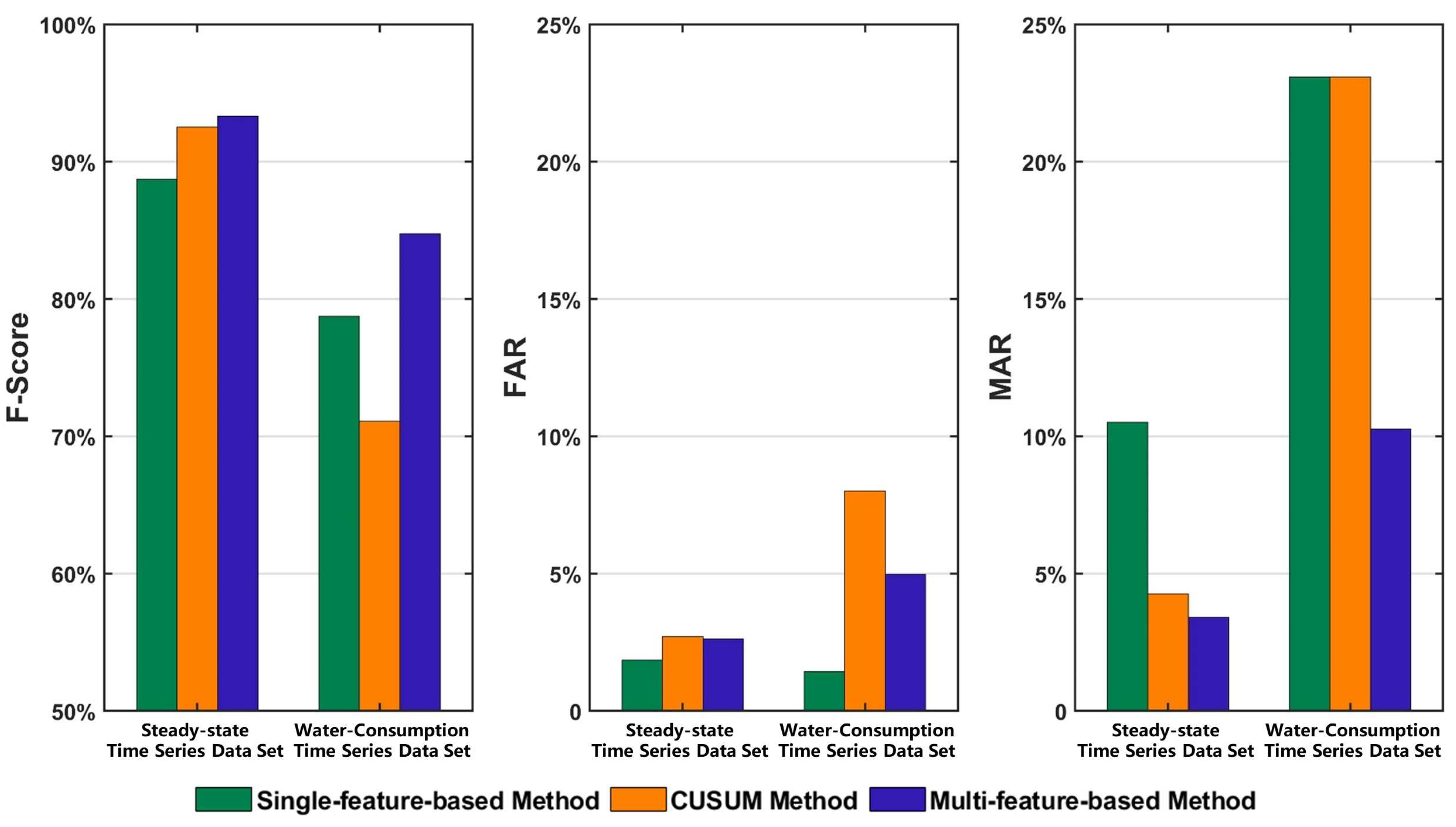
The final leakage detection performance results based on three different methods are shown in Figure 12. The single-feature-based method achieved a lower leakage detection performance on the steady-state time series data set but a better leakage detection performance on the water-consumption time series data set than the CUSUM method. It is shown that different characteristics are suitable for different network environments. ICs show better adaptability in network environments with obvious variations in water consumption, and the statistical characteristics extracted via the CUSUM method show the opposite. The proposed multi-feature-based method achieved better F-Scores for leakage detection on both of the time series data sets compared to the other two methods. Considering that the steady-state time series data set simulates a network environment during the night and that the water-consumption time series data set simulates a network environment in the daytime, the results for leakage detection show that the proposed multi-feature-based method can achieve better performance in different network environments and thus have more practical value in actual WDNs than the other two methods.
4. Conclusions
A leakage detection method based on multi-feature extraction from high-frequency pressure data has been proposed in this paper. The instantaneous and trend characteristics of leakage signals were extracted and analyzed for the detection of leakage events. The proposed method was verified in an experimental network with the interference of water consumption fluctuations.
The proposed method provides a new idea for leakage detection based on the extraction of comprehensive leakage information with two different kinds of characteristics. The data distributions of leakage time series data sets and leakage-free time series data sets were analyzed, the levels of pressure fluctuations in the network environments were quantified, and reasonable thresholds for leakage diagnosis were set in the paper. The results show that the proposed method has better adaptability to the pressure fluctuations in networks with different working conditions and that it achieves better accuracy and reliability in leakage detection in comparison to the single-feature-based method and the CUSUM method. The levels of pressure fluctuations were quantified and analyzed, providing an applicable reference for reasonable threshold settings of leakage diagnosis in a complex network environment. In addition, the prediction of leakage degree can be realized based on correlation analysis of the leakage characteristics and the flow rates of leakage events, which can assist a water company to take the proper response level of leakage repair.
This study has certain limitations, as it was conducted on an experimental network setup, where the simulation of variations in water consumption cannot fully reflect the patterns of water consumption in real WDNs. Therefore, the adaptability of the proposed method could be improved by further experiments with real WDNs. In future research, a small section of a real WDN should be considered as the research area and monitored with high-frequency pressure sensors at different locations. Combined with different working conditions and characteristics of water consumption, the levels and patterns of background pressure fluctuations in the research area should be evaluated and analyzed, and the setting of thresholds should be optimized to enhance the robustness of the proposed method for real WDNs.
Author Contributions
Writing—original draft preparation, X.W.; writing—review and editing, S.P.; software, resources, G.Z.; data curation, X.F.; project administration, Y.T. All authors have read and agreed to the published version of the manuscript.
Funding
This research was funded by the National Key R&D Program of China, grant number 2022YFC3203803.
Data Availability Statement
The data used in this manuscript are available from the corresponding authors.
Acknowledgments
Thanks to the National Key R&D Program of China for supporting and funding this project, grant number 2022YFC3203803.
Conflicts of Interest
The authors declare no conflict of interest.
References
- Che, T.-C.; Duan, H.-F.; Lee, P.J. Transient wave-based methods for anomaly detection in fluid pipes: A review. Mech. Syst. Signal Proc. 2021, 160, 107874. [Google Scholar] [CrossRef]
- Duan, H.-F.; Pan, B.; Wang, M.; Chen, L.; Zheng, F.; Zhang, Y. State-of-the-art review on the transient flow modeling and utilization for urban water supply system (UWSS) management. J. Water Supply Res. Technol. Aqua 2020, 69, 858–893. [Google Scholar] [CrossRef]
- Liemberger, R.; Wyatt, A. Quantifying the global non-revenue water problem. Water Supply 2019, 19, 831–837. [Google Scholar] [CrossRef]
- Feng, Y.-X.; Zhang, H.; Rad, S.; Yu, X.-Z. Visual analytic hierarchical process for in situ identification of leakage risk in urban water distribution network. Sustain. Cities Soc. 2021, 75, 103297. [Google Scholar] [CrossRef]
- Huang, Y.; Zheng, F.; Kapelan, Z.; Savic, D.; Duan, H.-F.; Zhang, Q. Efficient Leak Localization in Water Distribution Systems Using Multistage Optimal Valve Operations and Smart Demand Metering. Water Resour. Res. 2020, 56, e2020WR028285. [Google Scholar] [CrossRef]
- Fox, S.; Shepherd, W.; Collins, R.; Boxall, J. Experimental Quantification of Contaminant Ingress into a Buried Leaking Pipe during Transient Events. J. Hydraul. Eng. 2016, 142, 4015036. [Google Scholar] [CrossRef]
- Pudar Ranko, S.; Liggett James, A. Leaks in Pipe Networks. J. Hydraul. Eng. 1992, 118, 1031–1046. [Google Scholar] [CrossRef]
- Beck, S.B.; Curren, M.D.; Sims, N.D.; Stanway, R. Pipeline Network Features and Leak Detection by Cross-Correlation Analysis of Reflected Waves. J. Hydraul. Eng. 2005, 131, 715–723. [Google Scholar] [CrossRef] [Green Version]
- Sattar, A.M.; Chaudhry, M.H. Leak detection in pipelines by frequency response method. J. Hydraul. Res. 2008, 46, 138–151. [Google Scholar] [CrossRef]
- Li, Y.-B.; Sun, L.-Y. Leakage detection and location for long range oil pipeline using negative pressure wave technique. In Proceedings of the 2009 4th IEEE Conference on Industrial Electronics and Applications, Xi’an, China, 25–27 May 2009; pp. 3220–3224. [Google Scholar]
- Gong, J.; Lambert Martin, F.; Simpson Angus, R.; Zecchin Aaron, C. Single-Event Leak Detection in Pipeline Using First Three Resonant Responses. J. Hydraul. Eng. 2013, 139, 645–655. [Google Scholar] [CrossRef] [Green Version]
- Lin, J.; Wang, X.; Ghidaoui, M.S. Multi-Sensor Fusion for Transient-Based Pipeline Leak Localization in the Dempster-Shafer Evidence Framework. Water Resour. Res. 2021, 57, e2021WR029926. [Google Scholar] [CrossRef]
- Pan, B.; Duan, H.-F.; Keramat, A.; Meniconi, S.; Brunone, B. Efficient Pipe Burst Detection in Tree-Shape Water Distribution Networks Using Forward-Backward Transient Analysis. Water Resour. Res. 2022, 58, e2022WR033465. [Google Scholar] [CrossRef]
- Hampson, W.J.; Collins, R.P.; Beck, S.B.M.; Boxall, J.B. Transient Source Localization Methodology and Laboratory Validation. Procedia Eng. 2014, 70, 781–790. [Google Scholar] [CrossRef] [Green Version]
- Tijani, I.A.; Abdelmageed, S.; Fares, A.; Fan, K.H.; Hu, Z.Y.; Zayed, T. Improving the leak detection efficiency in water distribution networks using noise loggers. Sci Total Environ. 2022, 821, 153530. [Google Scholar] [CrossRef]
- Zhang, Y.; Jiang, Z.; Lu, J. Research on Leakage Location of Pipeline Based on Module Maximum Denoising. Appl. Sci. 2023, 13, 340. [Google Scholar] [CrossRef]
- Yang, Z.; Xiong, Z.; Shao, M. A new method of leak location for the natural gas pipeline based on wavelet analysis. Energy 2010, 35, 3814–3820. [Google Scholar] [CrossRef]
- Rashid, S.; Qaisar, S.; Saeed, H.; Felemban, E. A Method for Distributed Pipeline Burst and Leakage Detection in Wireless Sensor Networks Using Transform Analysis. Int. J. Distrib. Sens. Netw. 2014, 10, 939657. [Google Scholar] [CrossRef] [Green Version]
- Ferrante, M.; Brunone, B. Pipe system diagnosis and leak detection by unsteady-state tests. 2. Wavelet analysis. Adv. Water Resour. 2003, 26, 107–116. [Google Scholar] [CrossRef]
- Lu, X.; Sang, Y.; Zhang, J.; Fan, Y. A Pipeline Leakage Detection Technology based on Wavelet Transform Theory. In Proceedings of the 2006 IEEE International Conference on Information Acquisition, Veihai, China, 20–23 August 2006; pp. 1432–1437. [Google Scholar]
- Srirangarajan, S.; Allen, M.; Preis, A.; Iqbal, M.; Lim, H.B.; Whittle, A.J. Wavelet-based Burst Event Detection and Localization in Water Distribution Systems. J. Signal Proc. Syst. 2012, 72, 1–16. [Google Scholar] [CrossRef] [Green Version]
- Butterfield, J.D.; Collins, R.P.; Beck, S.B.M. Feature Extraction of Leaks Signals in Plastic Water Distribution Pipes Using the Wavelet Transform. In Proceedings of the ASME 2015 International Mechanical Engineering Congress and Exposition, Houston, TX, USA, 13–19 November 2015. [Google Scholar]
- Wang, S.; Chen, Z.; Wang, J.; Wang, H.; Ji, C.; Hong, J.; Gao, L. Continuous Leak Detection and Location through the Optimal Mother Wavelet Transform to AE Signal. J. Pipeline Syst. Eng. Pract. 2020, 11, 4020024. [Google Scholar] [CrossRef]
- Meng, T.; Wang, D.; Jiao, J.; Li, X. Tunable Q-factor wavelet transform of acoustic emission signals and its application on leak location in pipelines. Comput. Commun. 2020, 154, 398–409. [Google Scholar] [CrossRef]
- Ting, L.L.; Tey, J.Y.; Tan, A.C.; King, Y.J.; Abd Rahman, F. Water leak location based on improved dual-tree complex wavelet transform with soft thresholding de-noising. Appl. Acoust. 2021, 174, 107751. [Google Scholar] [CrossRef]
- Misiunas, D.; Lambert, M.; Simpson, A.; Olsson, G. Burst detection and location in water distribution networks. Water Supply 2005, 5, 71–80. [Google Scholar] [CrossRef]
- Kim, Y.; Lee, S.J.; Park, T.; Lee, G.; Suh, J.C.; Lee, J.M. Robust leak detection and its localization using interval estimation for water distribution network. Comput. Chem. Eng. 2016, 92, 1–17. [Google Scholar] [CrossRef]
- Ahmad, Z.; Nguyen, T.-K.; Kim, J.-M. Leak detection and size identification in fluid pipelines using a novel vulnerability index and 1-D convolutional neural network. Eng. Appl. Comput. Fluid Mech. 2023, 17, 2165159. [Google Scholar] [CrossRef]
- Zadkarami, M.; Shahbazian, M.; Salahshoor, K. Pipeline leak diagnosis based on wavelet and statistical features using Dempster–Shafer classifier fusion technique. Process Saf. Environ. Prot. 2017, 105, 156–163. [Google Scholar] [CrossRef]
- Aljameel, S.S.; Alomari, D.M.; Alismail, S.; Khawaher, F.; Alkhudhair, A.A.; Aljubran, F.; Alzannan, R.M. An Anomaly Detection Model for Oil and Gas Pipelines Using Machine Learning. Computation 2022, 10, 138. [Google Scholar] [CrossRef]
- Tian, X.; Jiao, W.; Liu, T.; Ren, L.; Song, B. Leakage detection of low-pressure gas distribution pipeline system based on linear fitting and extreme learning machine. Int. J. Press. Vessel. Pip. 2021, 194, 104553. [Google Scholar] [CrossRef]
- Wang, X.; Guo, G.; Liu, S.; Wu, Y.; Xu, X.; Smith, K. Burst Detection in District Metering Areas Using Deep Learning Method. J. Water Resour. Plan. Manag. 2020, 146, 4020031. [Google Scholar] [CrossRef]
- Bentoumi, M.; Chikouche, D.; Mezache, A.; Bakhti, H. Wavelet DT method for water leak-detection using a vibration sensor: An experimental analysis. IET Signal Proc. 2017, 11, 396–405. [Google Scholar] [CrossRef]
- Zhao, Y.; Wang, Q.; Ling, Z. Leakage detection and location analysis of tap water pipe based on distributed optical fiber temperature measurement. In Proceedings of the 10th International Conference on Information Optics and Photonics, Beijing, China, 8–11 July 2018. [Google Scholar]
- Jiang, Y.; Wang, B.; Li, X.; Liu, D.; Wang, Y.; Huang, Z. A Model-Based Hybrid Ultrasonic Gas Flowmeter. IEEE Sens. J. 2018, 18, 4443–4452. [Google Scholar] [CrossRef]
- Robertson, D.G.E.; Dowling, J.J. Design and responses of Butterworth and critically damped digital filters. J. Electromyogr. Kinesiol. 2003, 13, 569–573. [Google Scholar] [CrossRef]
- Fereidooni, Z.; Tahayori, H.; Bahadori-Jahromi, A. A hybrid model-based method for leak detection in large scale water distribution networks. J. Ambient Intell. Humaniz. Comput. 2020, 12, 1613–1629. [Google Scholar] [CrossRef]
Figure 1.
The framework of leakage detection.

Figure 2.
Experimental network system.

Figure 3.
Definition of the total duration of IC.

Figure 4.
Statistical distribution of the total duration of IC.

Figure 5.
Leakage detection performance for the steady-state time series data set under different threshold coefficients.
Figure 5.
Leakage detection performance for the steady-state time series data set under different threshold coefficients.

Figure 6.
Leakage detection performance for the water-consumption time series data set under different threshold coefficients.
Figure 6.
Leakage detection performance for the water-consumption time series data set under different threshold coefficients.

Figure 7.
Relationships between characteristic values of leakage events and leakage flow in the steady-state time series data set.
Figure 7.
Relationships between characteristic values of leakage events and leakage flow in the steady-state time series data set.

Figure 8.
Relationships between characteristic values of leakage events and leakage flow in the water-consumption time series data set.
Figure 8.
Relationships between characteristic values of leakage events and leakage flow in the water-consumption time series data set.

Figure 9.
Leakage degree prediction results: (a) the steady-state time series data set; (b) the water-consumption time series data set.
Figure 9.
Leakage degree prediction results: (a) the steady-state time series data set; (b) the water-consumption time series data set.

Figure 10.
The distribution of pressure drop levels in leakage-free time series in two time series data sets.
Figure 10.
The distribution of pressure drop levels in leakage-free time series in two time series data sets.

Figure 11.
The influence of the threshold coefficient on leakage detection performance in two time series data sets based on two methods: (a) the single-feature-based method on the steady-state time series data set; (b) the single-feature-based method on the water-consumption time series data set; (c) the CUSUM method on the steady-state time series data set; (d) the CUSUM method on the water-consumption time series data set.

Figure 12.
Comparison of F-Scores, FARs, and MARs of the different methods.


Table 1.
Confusion matrix.
| Label | Output | |
|---|---|---|
| L | NL | |
| L | TP | FN |
| NL | FP | TN |
Notes: TP = True Positive; TN = True Negative; FN = False Negative; FP = False Positive.
Table 2.
Leakage detection results for two time series data sets.
| Time Series Data Set Name | FAR | MAR |
|---|---|---|
| Steady-State Time Series Data Set | 2.63% | 3.41% |
| Water-Consumption Time Series Data Set | 4.97% | 10.26% |
Table 3.
Threshold coefficients in two time series data sets.
| Time Series Data Set Name | αic | αtc |
|---|---|---|
| Steady-State Time Series Data Set | 0 | 3 |
| Water-Consumption Time Series Data Set | 1 | 2 |
Disclaimer/Publisher’s Note: The statements, opinions and data contained in all publications are solely those of the individual author(s) and contributor(s) and not of MDPI and/or the editor(s). MDPI and/or the editor(s) disclaim responsibility for any injury to people or property resulting from any ideas, methods, instructions or products referred to in the content. |
© 2023 by the authors. Licensee MDPI, Basel, Switzerland. This article is an open access article distributed under the terms and conditions of the Creative Commons Attribution (CC BY) license (https://creativecommons.org/licenses/by/4.0/).
Share and Cite
MDPI and ACS Style
Wu, X.; Peng, S.; Zheng, G.; Fang, X.; Tian, Y. Leakage Detection in Water Distribution Networks Based on Multi-Feature Extraction from High-Frequency Pressure Data. Water 2023, 15, 1187. https://doi.org/10.3390/w15061187
AMA Style
Wu X, Peng S, Zheng G, Fang X, Tian Y. Leakage Detection in Water Distribution Networks Based on Multi-Feature Extraction from High-Frequency Pressure Data. Water. 2023; 15(6):1187. https://doi.org/10.3390/w15061187
Chicago/Turabian StyleWu, Xingqi, Sen Peng, Guolei Zheng, Xu Fang, and Yimei Tian. 2023. "Leakage Detection in Water Distribution Networks Based on Multi-Feature Extraction from High-Frequency Pressure Data" Water 15, no. 6: 1187. https://doi.org/10.3390/w15061187
Note that from the first issue of 2016, this journal uses article numbers instead of page numbers. See further details here.