Early Detection and Identification of Damage in In-Service Waterworks Pipelines Based on Frequency-Domain Kurtosis and Time-Shift Coherence

Abstract

Buried pipelines, such as waterworks pipelines, are critical for transmitting essential resources and energy in modern cities, but the risk of pipeline failure, especially due to third-party interference, is a major concern. While various studies have focused on leak detection in waterworks pipelines, research on preventing impact damage is limited. To address this issue, this study proposes a novel algorithm that utilizes energy and similarity measurements for impact detection and compares it theoretically to existing leak-detection methods. The proposed algorithm utilizes frequency-domain kurtosis to determine the frequency band on which the energy of the impact signals is concentrated, along with a time-shift coherence function to measure the similarity of the signals. The application of the source location using the filtered signals enables accurate detection of the location of third-party interference. The proposed algorithm aims to ensure the safety and to prevent failures of buried pipelines. To verify the feasibility of the proposed algorithm, an excavation experiment using a backhoe was conducted on an in-service waterworks pipeline with a diameter of 2200 mm and a burial depth of 3 m. This experiment confirmed the effectiveness of the proposed algorithm in preventing failures of buried pipelines and demonstrated its practical applicability in the field. The experiment also validated the algorithm’s ability to detect third-party interference damage at various points.

1. Introduction

Buried pipeline networks, such as in-service waterworks pipelines, are crucial components of modern cities that support industrial and residential activities by transmitting essential resources and energy. Moreover, buried pipeline networks have become increasingly complex as cities continue to develop and the demand for resources and energy increases. Therefore, the issue of pipeline failure becomes a critical problem that must be addressed in order to maintain the functionality of cities, and it is increasingly being prioritized. As a result, the risk of pipeline failure has become a major concern for cities and is receiving increased attention from the management agencies responsible for the pipeline networks, such as water, gas, and oil companies. It has been found that corrosion, material defects, third-party interference (TPI), and ground loads were the primary causes of buried pipeline failures [1,2,3]. Most problems can be prevented through proper maintenance and continuous management, but instances of TPI are not only unpreventable but also cause unexpected large-scale accidents [4,5]. Therefore, technology such as structural health monitoring is becoming increasingly important to ensure the reliability and integrity of buried pipeline networks, especially to prevent unexpected accidents caused by TPI.

The research on pipeline integrity was initiated with an emphasis on detecting leaks. Early-stage leak-detection methods relied on acoustical analyses by skilled experts utilizing listening rods, frequently producing incorrect results [6]. To overcome these limitations, leak-detection methods based on a correlation analysis were proposed [7]. As a result, while the detection range was limited to a few meters, leak detection based on a frequency-domain analysis became possible [8]. As the propagation speed of waves was understood to be a key variable in leak detection, researchers subsequently focused on conducting theoretical-mode analyses of fluid-filled pipelines. Theoretically, it was found that most of the energy in fluid-filled pipelines is transmitted through four waves [9]. Among them, the quasi-longitudinal wave was confirmed to be the most suitable for leak detection due to its ability to propagate over long distances [10]. Moreover, the theoretical description of the dependence of the propagation speed of quasi-longitudinal waves on the physical properties and burial environment of pipelines allowed for more accurate estimations of the propagation speed of these waves [11]. With consideration of the factors mentioned earlier, an algorithm for selecting the optimal frequency band for leak detection was proposed based on an analysis of the power spectral density (PSD) and coherence of the signals as obtained from sensors [12]. The effectiveness of this algorithm was demonstrated through experiments conducted on actual buried pipelines [8]. Thus, numerous studies are attempting to devise methods capable of detecting leaks in pipelines, from the development of theoretical models to experimental validation. Based on these research findings, various leakage detection studies have been conducted in different environments, and leakage detection technologies for monitoring the integrity of pipelines under onshore, offshore, subsea, and arctic conditions have been developed and applied [13]. However, the research on preventing pipeline failures due to impact damage such as TPI is relatively insufficient. In relation to damage caused by TPI, some studies are underway, such as a recent study related to impact-damage detection of pipelines, with an acoustic propagation model suggested for the initial detection of impacts that induce damage in gas pipelines. The feasibility of the algorithm was verified through lab-scale experiments [14]. In addition, the possibility of high-accuracy source location for damage detection was verified by applying the continuous wavelet transform in an environment with actual noise [15]. This study highlights the ongoing efforts to detect and prevent impact damage in pipelines. While research in this area is still limited, the proposed acoustic propagation model and the application of the continuous wavelet transform showed promising results in terms of the development of effective impact-damage detection systems. In conclusion, in order to prevent pipeline failures due to impact damage caused, for instance, by TPI, it is necessary to detect the activities that may cause such damage before they affect the pipelines.

In this study, a novel algorithm is proposed for early detection of pipeline failure by detecting ground excavation activities conducted on the surface above buried pipelines. The algorithm operates by utilizing energy and similarity measurements, similar to the methodology applied in well-developed leak-detection algorithms. The proposed approach identifies suitable factors for impact detection by observing the theoretical differences between leak signals and impact signals. Frequency-domain kurtosis (FDK) is used to determine the frequency band on which the energy of the impact signals is concentrated, and a time-shift coherence function is introduced to overcome the limitation of coherence functions in measuring the similarity of impact signals. With these elements combined, the proposed algorithm aims to ensure the safety and to detect failures of buried pipelines early.

This paper is organized as follows. In Section 2, a theoretical comparison is made between the proposed method and the conventional leak-detection method. The experimental setup for excavation using a backhoe on a surface where pipelines are buried is introduced in Section 3. Finally, the performance and verification results of the proposed algorithm are discussed in Section 4 based on the experimental results.

2. Source Localization of Impact Damage

2.1. Conventional Source Location of Leaks in Fluid-Filled Pipelines

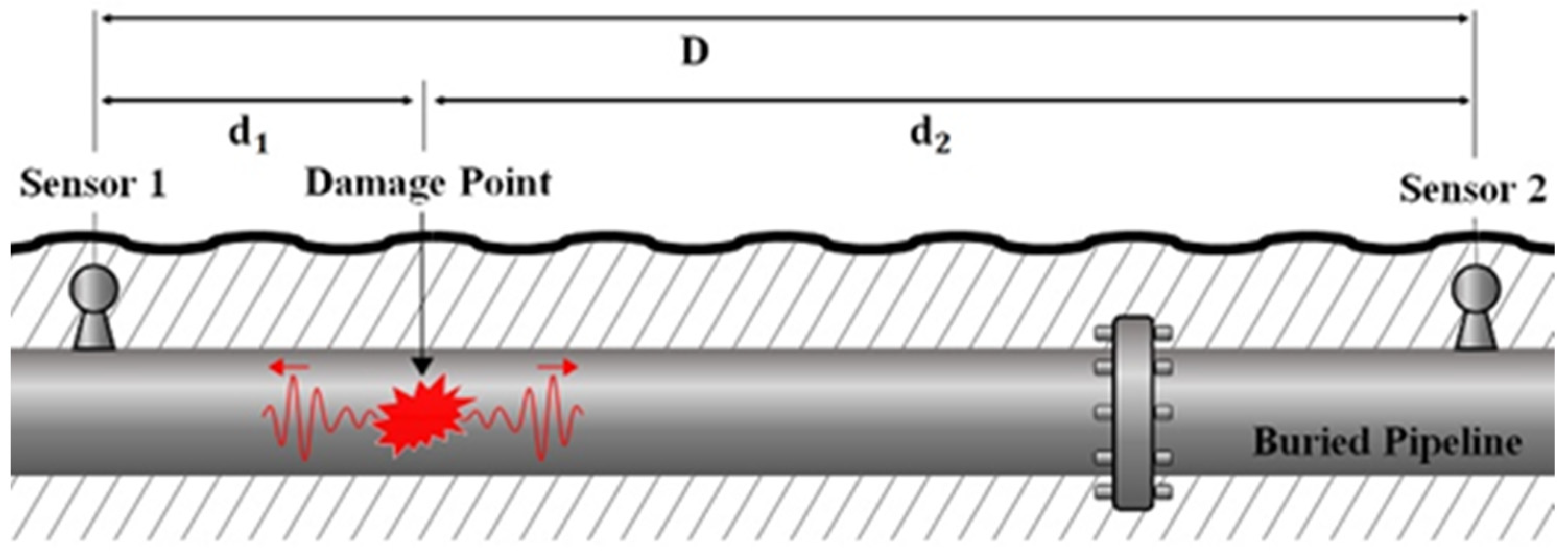
As previously mentioned, the majority of pipeline research has focused on leak detection. The method for pipeline leak detection is recognized as being applicable in the field. It utilizes two spatially separated sensors to identify the locations of leaks within the monitored area, as shown in Figure 1.

The position of a leak can be calculated using Equation (1):

$$d_{1,2}=\frac{1}{2}\left(D\pm c∆t\right)$$

(1)

where “$D$” denotes the distance between sensors or the monitoring range, “$c$” is the propagation speed of the leak sound, “$∆t$” is the difference in time when the wave reaches each sensor, and the “$d_{1,2}$” values are the results of the source location, representing the distance from the leakage point to each sensor.

The conventional leak-detection method involves filtering the signal through an optimal frequency band determined by observing the characteristics of the leak signal. The optimal frequency band is selected through an examination of the PSD and coherence, both of which are based on a frequency-domain analysis. The PSD measures the energy of the leak signal, while coherence measures the similarity of the signals. Therefore, the optimal frequency band is the frequency band that has high energy levels for both signals and high similarity between the two signals. This is an effective method of analyzing the characteristics of the signals obtained from two sensors to determine the presence of a leak. The time difference between the two filtered signals is then measured by means of cross-correlation to determine the location of the leak. The combination of selecting the optimal frequency band and measuring the time difference between signals is a highly effective means of detecting leaks in pipelines. Various methods that accurately estimate the time difference have been proposed [16], even in noisy conditions through the application of weighting functions [17] such as the maximum likelihood [18], the Roth processor [19], and smoothed coherence transform [20], in the cross-correlation process.

The wave propagation characteristics of fluid-filled pipelines have been studied extensively in the context of leak-detection research, with the aim of implementing long-range leak-detection systems. The research has focused on selecting a suitable wave based on a mode analysis. As a result, among the various waves that can be transmitted in fluid-filled pipelines, the quasi-longitudinal wave was found to be the most suitable type because the quasi-longitudinal wave is less attenuated than other waves due to its transmission through the fluid, resulting in a longer propagation distance [21]. Additionally, the interaction between the fluid and the elastic pipe leads to uniform contraction and expansion in all directions of the cross-section, making it easy to measure the quasi-longitudinal wave with a uniaxial sensor installed on the outside of the pipe.

The propagation speed of a quasi-longitudinal wave can be expressed as follows:

$$c=c_f{\left[1+\frac{\frac{2B_f}{a}}{\frac{Eh}{a^2}-\rho h{\omega }^2}\right]}^{-\frac{1}{2}}$$

(2)

where c_f, B_f, a, E, ρ, h, and ω denote the longitudinal wave speed of a fluid in free space, the bulk modulus of the internal fluid, the mean pipe radius, which is calculated based on the outer and inner diameter of a pipe, Young’s modulus of the pipe, the density of the pipe material, the pipe thickness, and the angular frequency, respectively.

Figure 2 shows the calculated propagation speed of the quasi-longitudinal wave using Equation (2), where the internal space is filled with fluid and the pipe material is steel. This figure indicates a significant difference in the wave speed compared to a non-dispersive wave propagating through a fluid in free space. Not only does it converge to 0 m/s, but it also shows characteristics where the speed variation range differs based on changes in the diameter. The frequency at which the speed converges to 0 m/s is referred to as the ring frequency. The ring frequency is known to be the frequency at which the wavelength of the quasi-longitudinal wave coincides with the circumference of the pipe. Thus, as the diameter increases, the ring frequency tends to decrease. Additionally, if the speed at 0 Hz is defined as the “initial speed”, it exhibits an inverse relationship with the diameter, as shown in Equation (2). In other words, as the diameter of a fluid-filled pipeline increases, the initial speed of the quasi-longitudinal wave propagating through it decreases, and the dispersion curve becomes steeper. Here, all the specifications for the material and dimension of the pipe used in Figure 2 were based on the American Society of Mechanical Engineers standard ASME B36.19M.

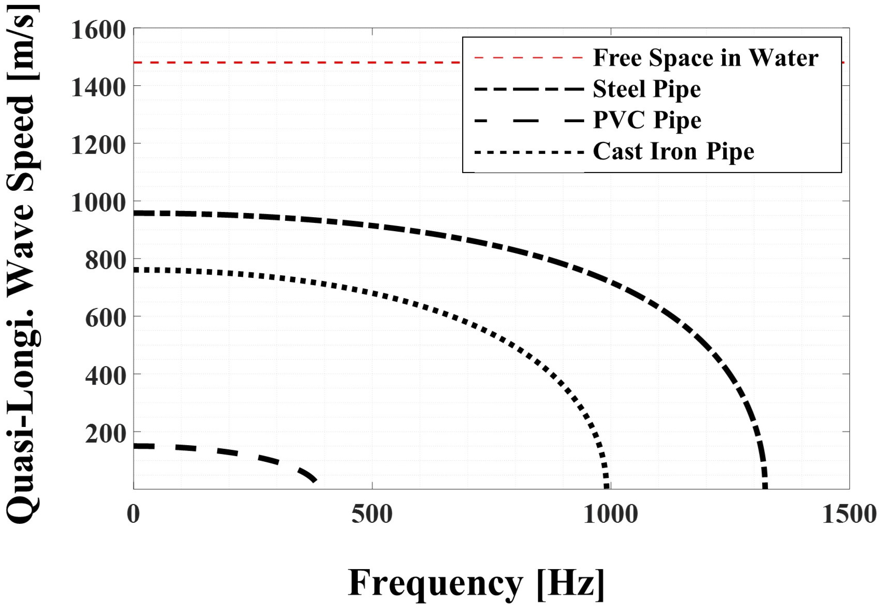
Figure 3 shows the propagation speed of a quasi-longitudinal wave calculated by Equation (2) for the different materials of pipe. The pipe diameter is fixed at 1200 mm for all materials. All three pipes were assumed to be water-filled, and the material properties of the pipes including the Young’s modulus and density were assumed to have nominal values. The results show that the quasi-longitudinal wave is formed by the interaction between fluid and the pipe, and, therefore, it can be seen that this varies greatly depending on the material and dimension of the pipe.

2.2. Source Location of Impact Damage in Fluid-Filled Buried Pipelines

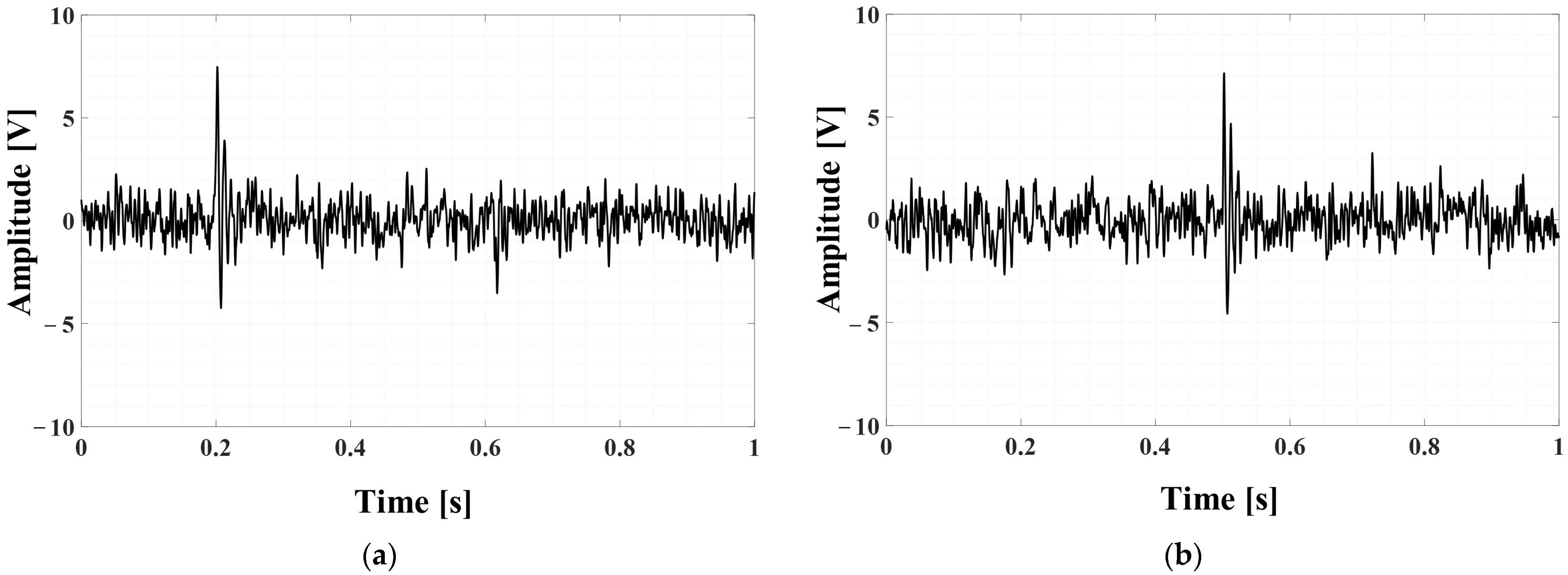
Due to the characteristics of fluid-filled pipelines, which determine the propagation form of energy, both TPI and leaks generate the same quasi-longitudinal wave. However, it is known that the shapes of the waveforms generated by TPI and by leakages differ significantly. Leak signals are typically continuous signals, while impact signals are typically transient signals. This difference suggests that algorithms designed for leak detection may not be suitable for detecting TPI and other impact damage. The reason for this is that while the leak signal is included over the entire time when observing PSD for the selection of the optimal frequency band, in the case of impact signals, it can only exist in part of the signal, leading to an inaccurate PSD. The coherence function measures the degree of similarity between two signals based on their phase relationship and assumes that the signals are stationary and have a constant phase relationship over time. However, if transient signals exist at different times, their phase relationship is not stationary and changes with time, which can lead to an incorrect estimation of coherence [22]. In summary, applying the PSD and coherence, which are known as observation data for selecting the optimal frequency band for leak detection [23], to impact signals, as shown in Figure 4a,b, may result in the phenomena discussed below. These signals, designed to reflect real scenarios, include white Gaussian noise as background noise, and the damage signal, represented in red, is designed as a damped sine wave with a center frequency of 100 Hz. It is assumed that the damage wave has a propagation speed of 1000 m/s and occurs at a position 200 m away from a total length of 700 m. Therefore, the virtual measurement signal x(t) shown in Figure 4a is composed of white Gaussian noise and an impact signal that occurs at approximately 0.2 s, while the virtual measurement signal y(t) shown in Figure 4b is designed as an impact signal occurring at approximately 0.5 s, along with white Gaussian noise. Accordingly, the time difference between the impact signals present in the two signals is designed to be approximately 0.3 s.

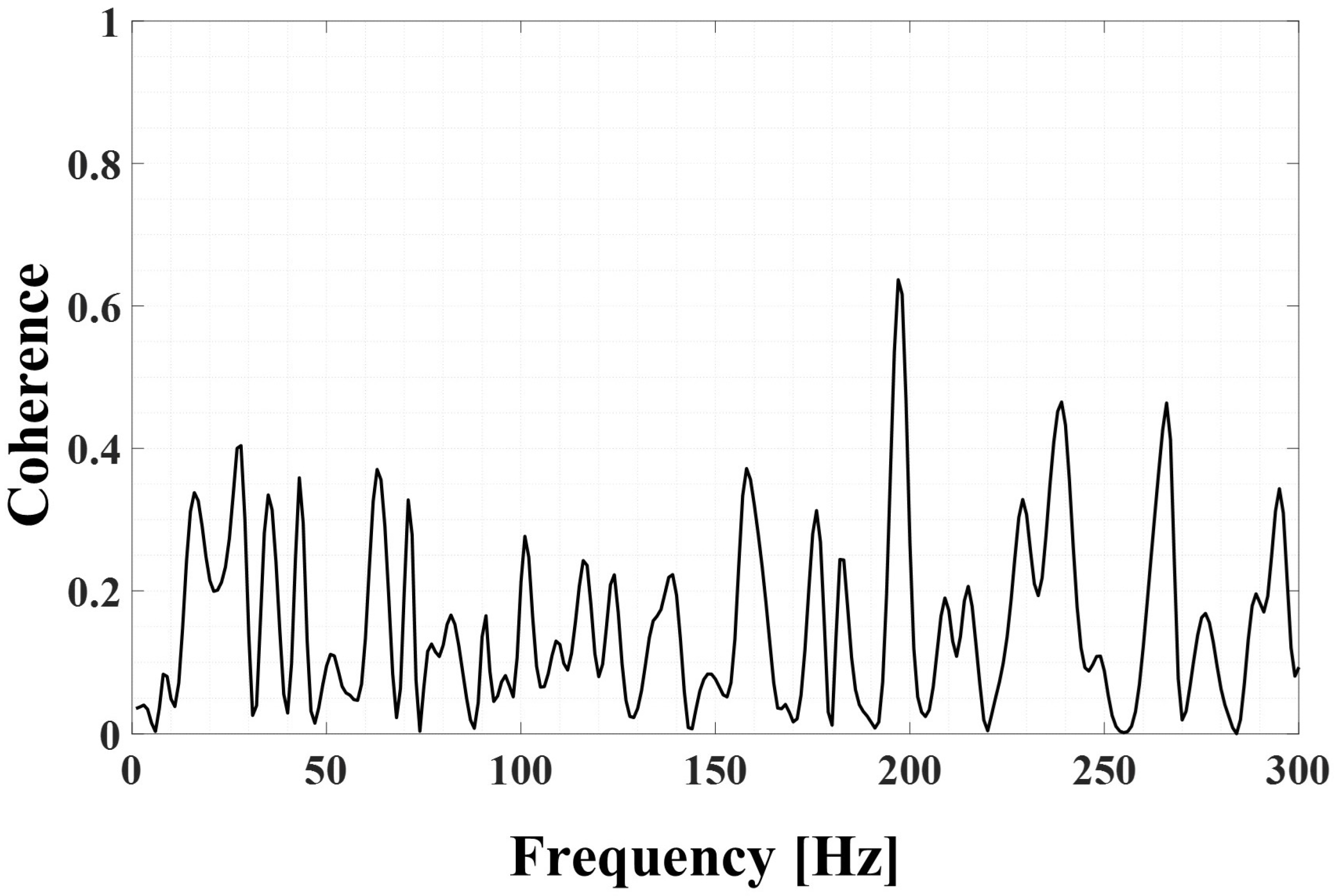
Figure 5a,b show the results after calculating the PSD of each of the two signals. Although the center frequency band is relatively high, it is difficult to clearly distinguish the optimal frequency band. Similarly, Figure 6 shows the coherence calculated using the two signals. Although both signals were designed to contain signals in the 100 Hz band, the results of the 100 Hz band for coherence show that there is no similarity between the two signals. Therefore, in this study, a new concept for impact-damage detection is proposed, where FDK is used for the energy observation, and time-shift coherence, which is a newly suggested function, is used for the similarity measurement instead of the well-developed energy (PSD) and similarity (coherence) measurement concepts, which are not suitable for TPI or other impact-damage detection approaches.

FDK was proposed by Dwyer to detect transient signals that are generated by ice cracks [24]. Furthermore, it was demonstrated that FDK is more effective when used to detect transient signals than the power spectrum density, which is a representative indicator for observations of signal characteristics [25]. Afterwards, FDK was reintroduced by Ottonello after being reorganized [26]. FDK can be calculated by Equation (3):

$$FDK\left(f\right)=\frac{\frac{1}{M}{\sum }_{i=1}^M{\left|S_i\left(f\right)\right|}^4}{{\left[\frac{1}{M}{\sum }_{i=1}^M{\left|S_i\left(f\right)\right|}^2\right]}^2}$$

(3)

Here, M represents the number of segments into which the signal samples have been divided for the purpose of estimating discrete Fourier transform (DFT), while $S_i\left(f\right)$ refers to the ith segment obtained after dividing the signal samples used in the estimation of DFT.

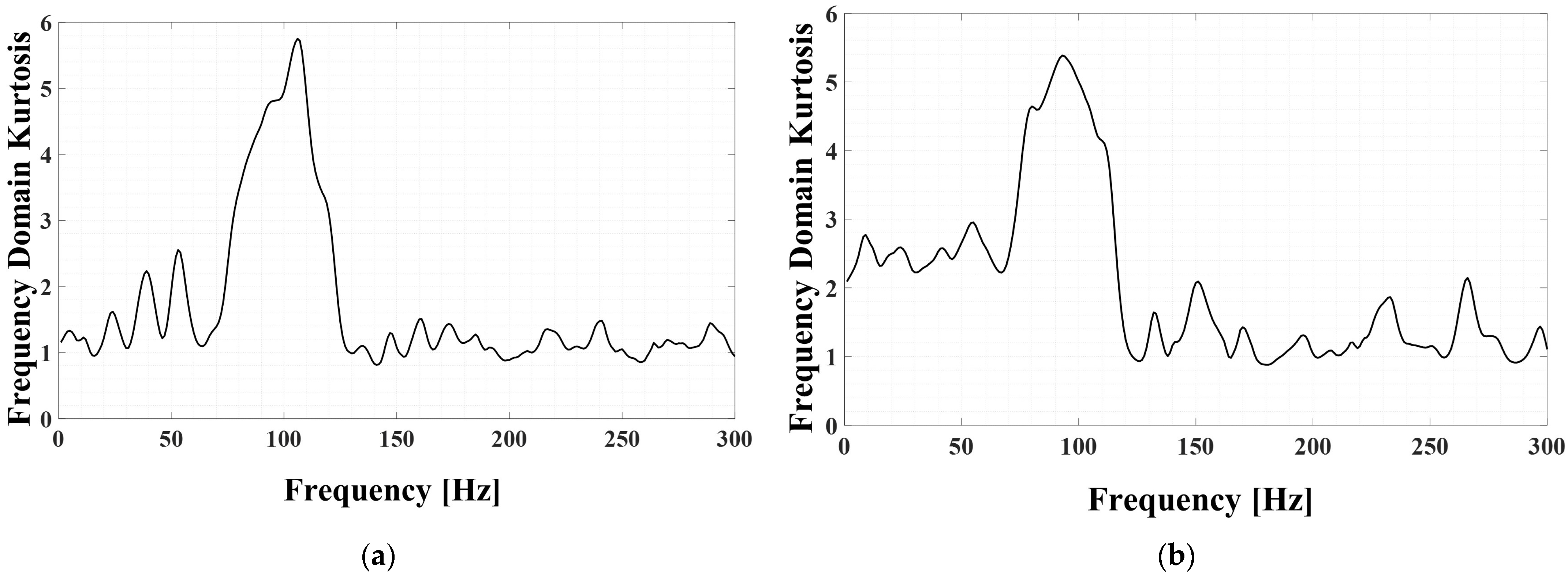
Figure 7a,b show the results when applying FDK to each signal shown in Figure 4. Compared to the PSD shown previously, it is clear that the main frequency band of 100 Hz can be easily distinguished. Unlike the PSD, which is directly related to the energy, FDK is a statistical variable that can be used as an indirect indicator of the energy because it allows for the identification of frequency bands containing transient signals.

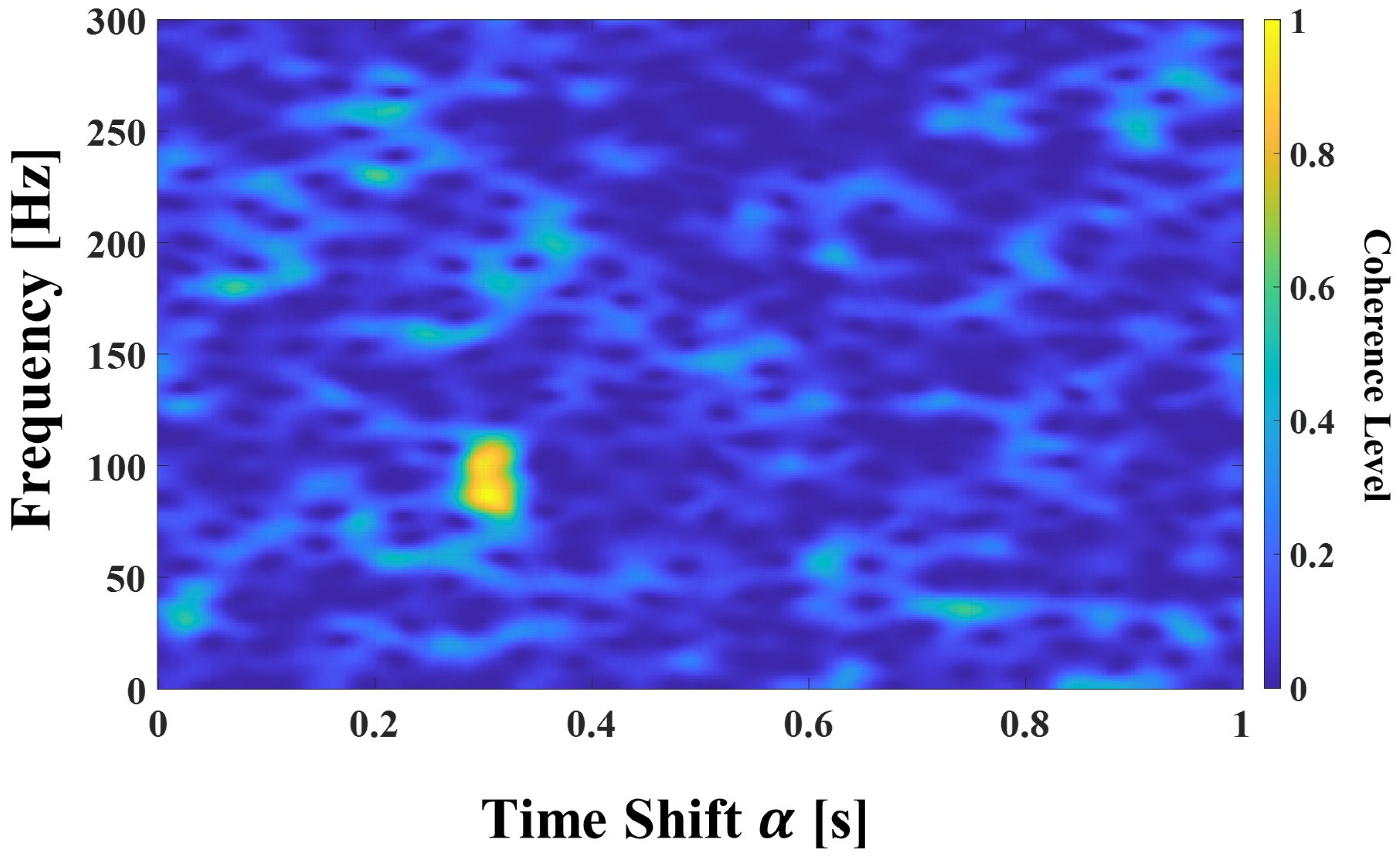
For the purpose of measuring the similarity of impact damage signals, this study proposes a new method called time-shift coherence, $T{C}_{xy}\left(f,a\right)$. This function is specifically designed to measure the similarity of transient signals by taking into account the time shift between them. Unlike the traditional coherence function, which may yield inaccurate results when applied to transient signals, the $T{C}_{xy}\left(f,a\right)$ function takes the time shift into consideration, enabling accurate similarity measurements of transient signals.

$T{C}_{xy}\left(f,a\right)$ can be calculated by the process defined below.

First, we assume the existence of two transient signals, x(t) and y(t), as shown in Figure 4. The originally coherence, which used two signals, can be expressed by Equation (4):

$$Coherence \left(x\left(t\right), y\left(t\right)\right)=C_{xy}\left(f\right)=\frac{{\left|G_{xy}\left(f\right)\right|}^2}{G_{xx}\left(f\right)\ast G_{yy}\left(f\right)}$$

(4)

where $G_{xy}\left(f\right)$ is the coherence function, $G_{xy}\left(f\right)$ denotes the cross-power spectrum, $G_{xx}\left(f\right)$ is the power spectrum of signal $x\left(t\right)$, and $G_{yy}\left(f\right)$ is the power spectrum of signal$y\left(t\right)$.

The time-shift signal, a signal that can be expressed as$y\left(t-a\right)$, is then moved in multiple steps and applied to the original coherence equation. Therefore, the original coherence can be modified to time-shift coherence, which is represented by Equation (5).

$$Time-shift coherence\left(x\left(t\right),y\left(t-a\right)\right)={TC}_{xy}\left(f,a\right)=\frac{{\left|G_{xy}\left(f,a\right)\right|}^2}{G_{xx}\left(f\right) \ast G_{yy}\left(f,a\right)}$$

(5)

where $T{C}_{xy}\left(f,a\right)$ is the time-shift coherence function of $x\left(t\right)$ and $y\left(t-a\right)$, $G_{xy}\left(f,a\right)$ is cross-power spectrum of$x\left(t\right)$ and$y\left(t-a\right)$, $\mathrm{and} G_{yy}\left(f,a\right)$ is the power spectrum of$y\left(t-a\right)$.

The time-shift coherence is expressed in two dimensions of the time-shift step(s)-frequency(f), and like the original coherence, it also represents the similarity between two signals as a value between 0 and 1. As a result, it is changed to a function that can approximately infer the similarity of transient signals that could not be calculated by the original coherence. Figure 8 shows the results after measuring the similarity of transient signals using the time-shift coherence. This suggests that the main frequency band of the transient signal can be easily identified, which is different from the results of the original coherence shown in Figure 6.

Hence, it is possible to improve the signal-to-noise ratio of the impact signal by selecting the main frequency band inferred through the FDK and $T{C}_{xy}\left(f,a\right)$ observations as the optimal frequency band and designing a bandpass filter. Figure 9 shows a bandpass filter signal with the optimal frequency band. This suggests that applying the approach proposed in this study can improve the signal-to-noise ratio of the transient signal expressed in red in Figure 4.

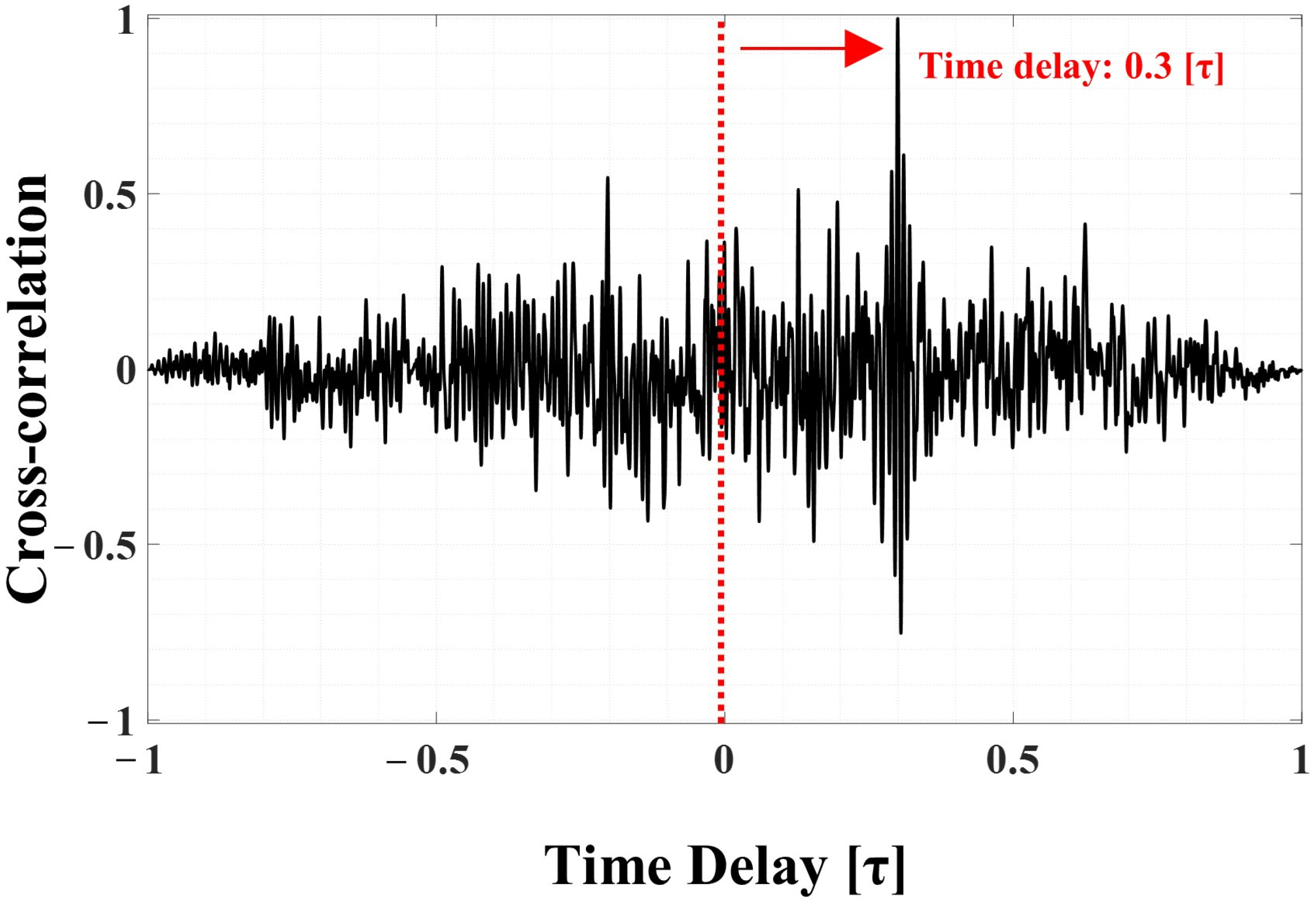
Moreover, Figure 10 shows the results of the cross-correlation for the time delay estimation using filtered signals. As a result, it can be seen that the previously designed delay time of 0.3 s can be recognized with high accuracy.

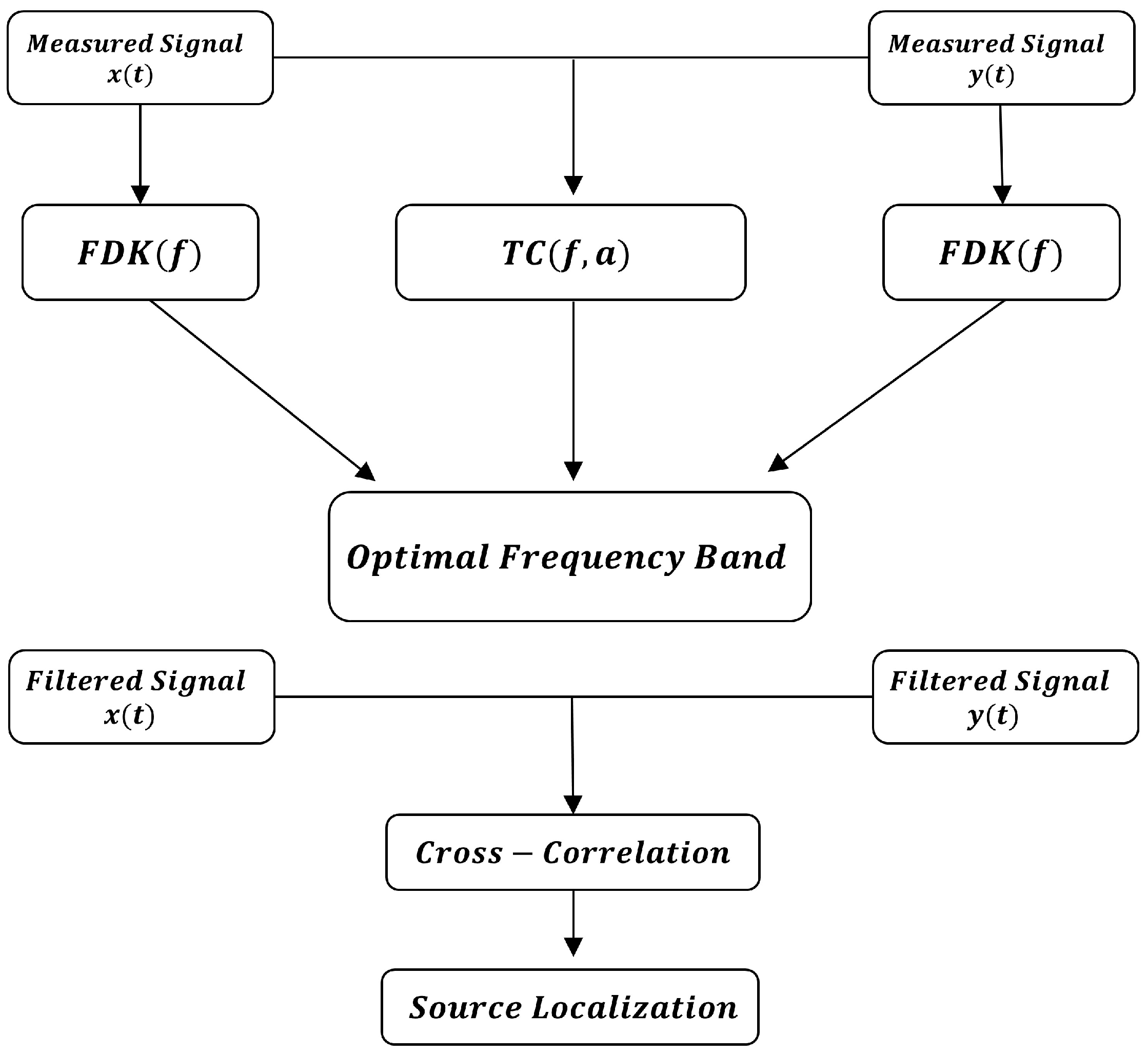
In summary, a schematic diagram of the series of processes described above is shown in Figure 11. This method, like a well-developed leak-detection technique, is considered to be a method capable of effectively detecting an impact on a buried pipeline. In particular, FDK calculates a frequency band where transient signals exist, and time-shift coherence reconfirms the frequency bands with high similarity between the two signals such that optimal frequency bandpass filters can be designed to filter only the main frequency bands of the impact signals. When estimating the arrival time difference based on the cross-correlation using the filtered signal, it is believed that the location of the impact signal can be effectively detected.

3. Experiments

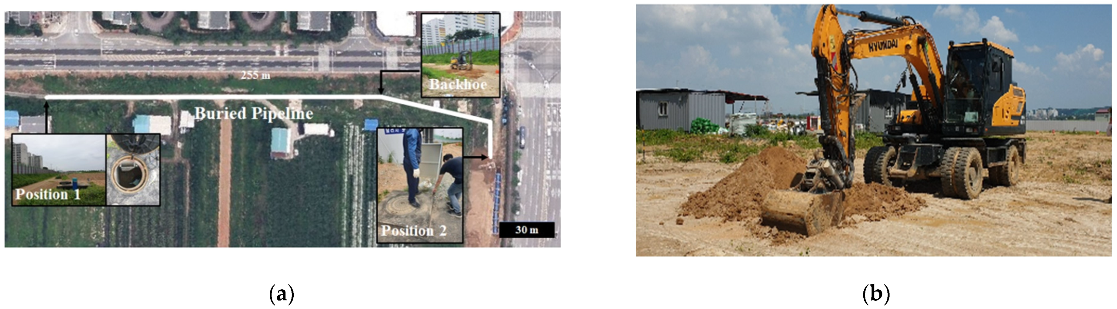
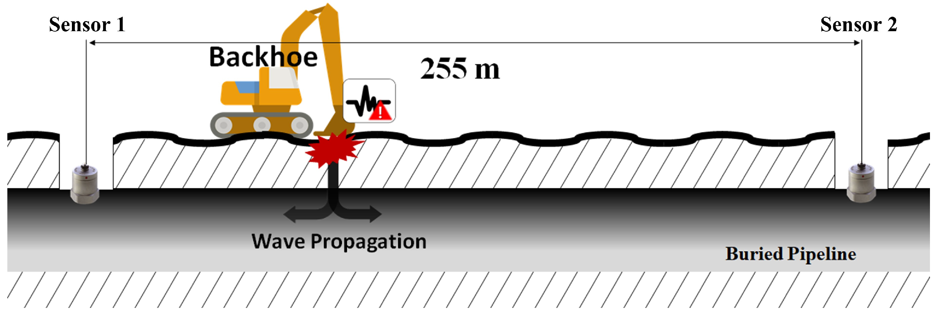
To validate the algorithm proposed for preventing pipeline damage due to TPI, experiments were conducted on in-service buried pipelines in O-Song, a city in Korea. A pipeline with a 2200 mm diameter buried approximately 3 m underground was used, with a 255 m section selected as the testbed, as shown in Figure 12a. To test the prevention of damage caused by TPI, backhoe excavation was performed on the ground where the pipeline was buried, as shown in Figure 12b. The impact energy applied to the ground was transmitted through the pipeline, and the aim was to detect this and prevent damage before a failure occurs, as shown in Figure 13.

Accelerometers with a sensitivity of 10 V/g were attached to both ends of the monitoring area, and for this, the National Instruments NI-9234 model was used. The signals were measured with a sampling frequency of 5.12 kHz in an environment with various types of noise, as the target pipeline was buried under a two-way eight-lane roadway and a parking lot.

Experiments were conducted at different locations, including 60 m, 80 m, 100 m, 125 m, 150 m, and 180 m out of the total 255 m section, as shown in Figure 12, to validate the proposed approach. The experiments were performed under different ground conditions, and the goal was to detect the actual excavation location by applying the proposed approach to the measured signals.

4. Results and Discussion

As described earlier, the optimal frequency band is selected by observing the FDK and $T{C}_{xy}\left(f,a\right)$ of the measured signals for impact signal detection. Subsequently, the signals are filtered using a bandpass filter designed on the optimal frequency band, and the arrival time difference of the impact signals is estimated by applying these filtered signals to the cross-correlation.

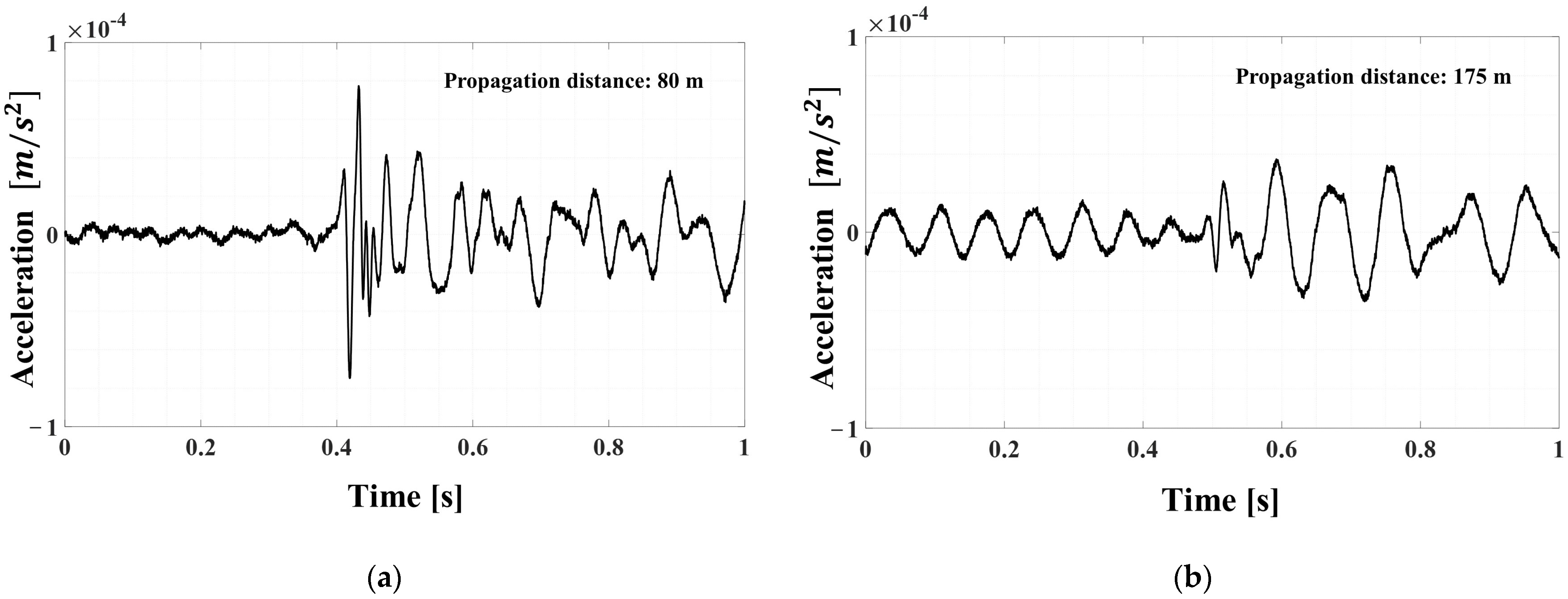
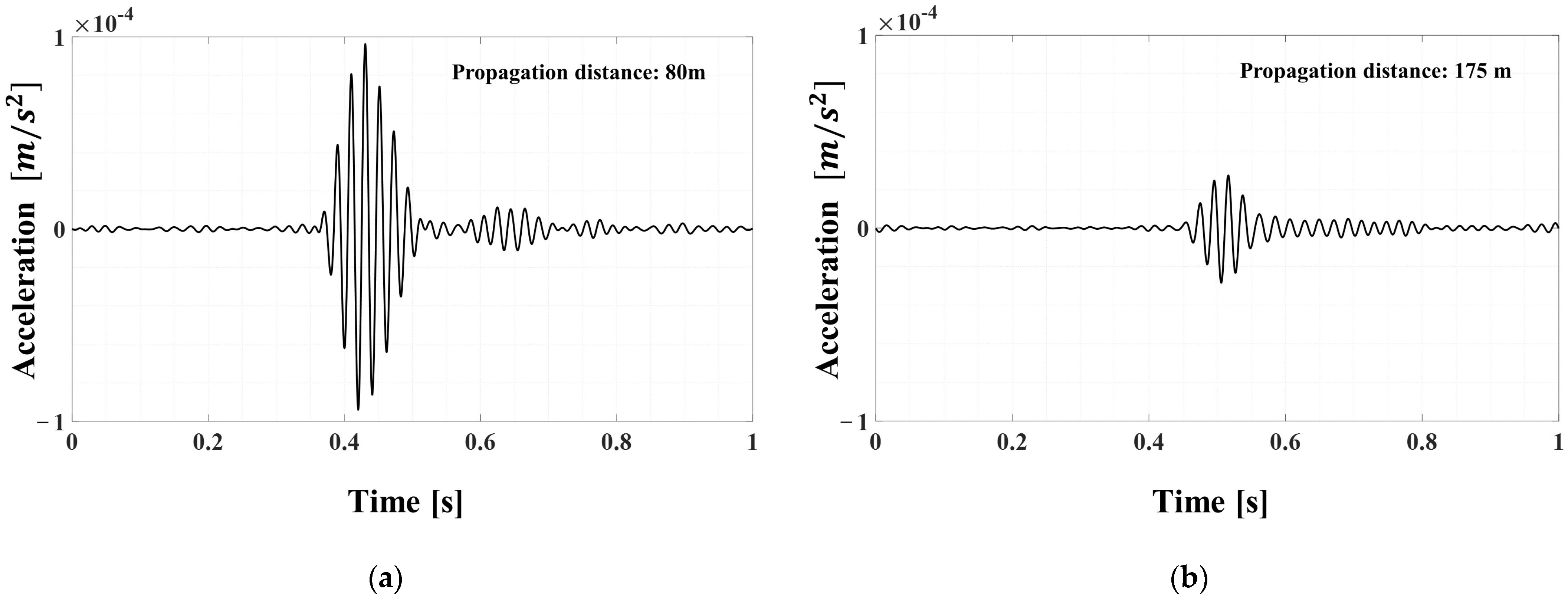
Figure 14a,b show the results of the signals generated during excavation activities at the 80 m position in the 255 m pipeline. Sensor 1 measures the signal that propagated from 80 m, as shown in Figure 14a, while sensor 2 measures the signal that propagated from 175 m, as shown in Figure 14b. In particular, the measurement signal of sensor 2 is exposed to various types of noise due to its proximity to the road. Therefore, as shown in Figure 14b, it can be seen that it is difficult to distinguish the impact signal from the noise due to the low signal-to-noise ratio in the raw signal. On the other hand, the measurement signal of sensor 1 in Figure 14a has a short propagation distance and is located in a relatively noise-free area, resulting in a high signal-to-noise ratio. This is a characteristic of typical field experiments, indicating that different conditions exist at each position, even in the same testbed.

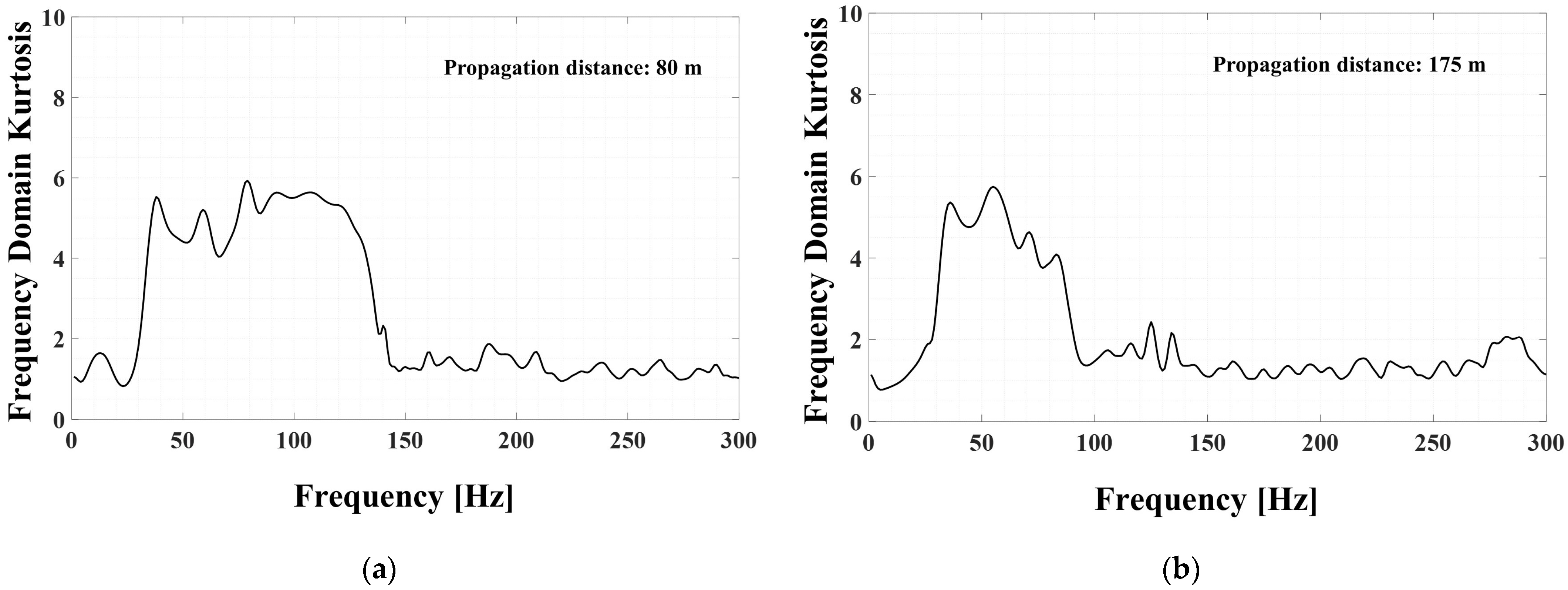
Figure 15a,b show the results of the FDK for the signals described earlier, serving as an indicator to find the dominant frequency band of the transient signal. Figure 15a shows the FDK results of the impact signal that propagated from 80 m, and it can be observed that the dominant frequency range is approximately 30 to 120 Hz. The FDK of the signal transmitted to sensor 2, which is located 175 m away, shows that the dominant frequency range is 30–90 Hz. Therefore, it can be seen that some high-frequency bands were attenuated as the wave propagated over a long distance.

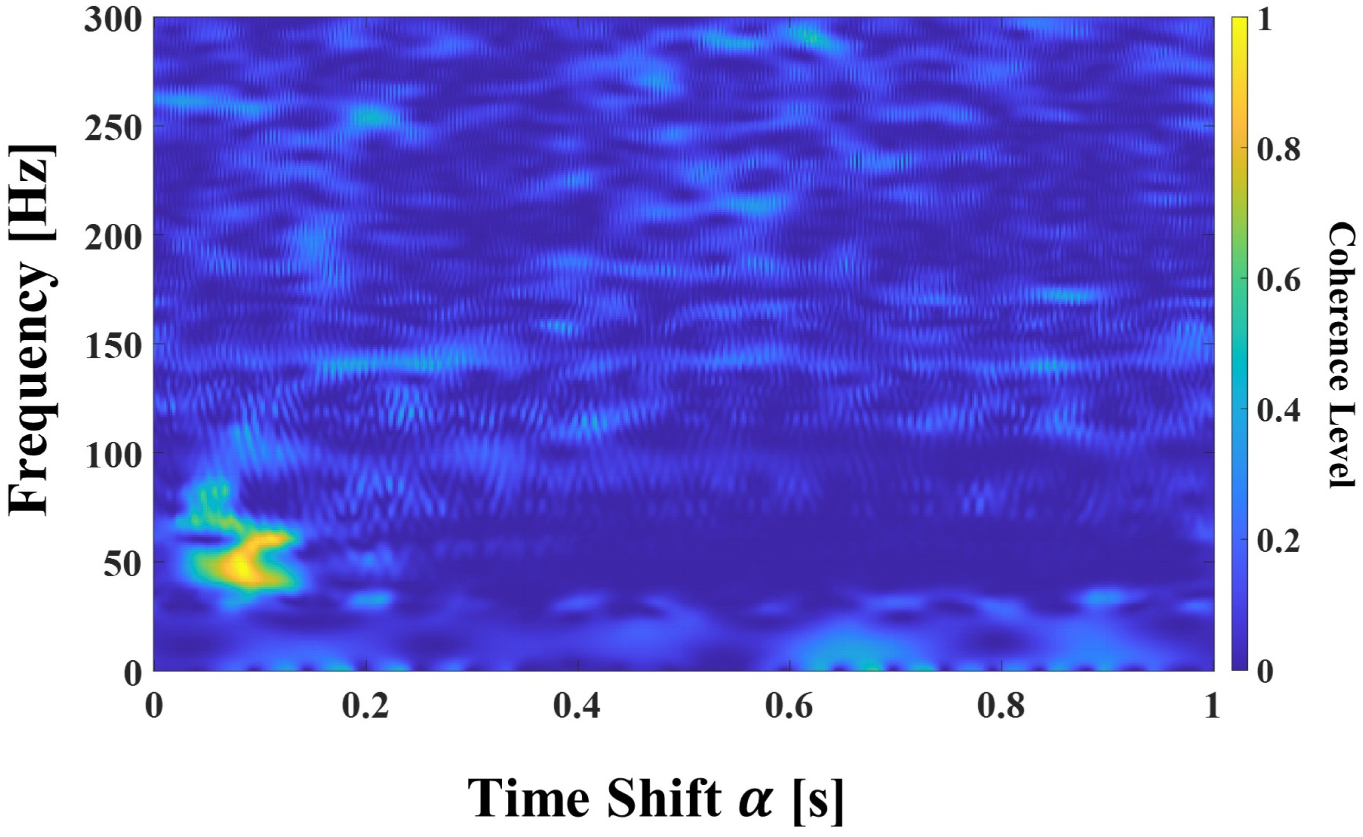
Figure 16 shows the results of the newly proposed $T{C}_{xy}\left(f,a\right)$ for a comparison of the similarities between the measured transient signals. The results of the proposed $T{C}_{xy}\left(f,a\right)$, as shown in Figure 16, indicate that the frequency band of 40–60 Hz, which is narrower than the 30–90 Hz frequency band that was determined as the optimal frequency band through the FDK observation, is the one with highest level of similarity.

As a result of these observations, the narrow frequency band of 40–60 Hz was selected as the optimal frequency band, rather than the wider 30–90 Hz frequency band that was initially considered as a candidate for the optimal frequency band based on the FDK observations. Figure 17a,b show the two signals filtered using the optimal frequency band. The results indicate that the signal-to-noise ratios of both signals have improved. In particular, for the signal propagated at 175 m, it can be seen that most of the noise has been removed.

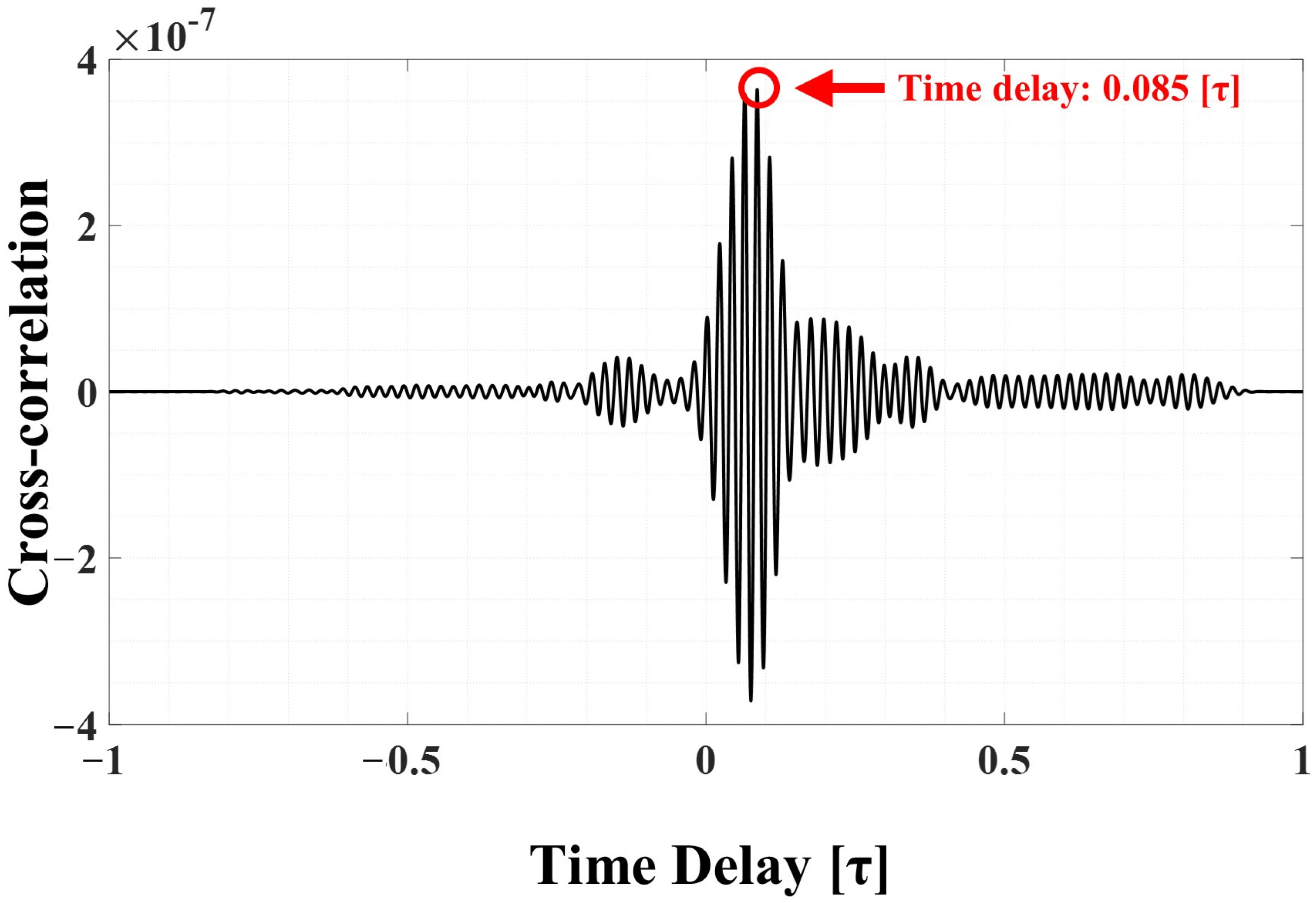
Figure 18 shows the calculation results of the cross-correlation using two signals with improved signal-to-noise ratios. As a result, it was confirmed that a time difference of approximately 0.085 s occurred between the two signals.

A characteristic of the speed of a quasi-longitudinal wave, which must be known when calculating the source location, is that it changes with the frequency, as depicted in Figure 2. The theoretical propagation speed at 40~60 Hz, which was selected as the optimal frequency band, was approximately 820 m/s.

Therefore, by applying the arrival time difference (0.085 s), the propagation speed (820 m/s), and the total distance (255 m) to Equation (1) to express the source location, the damage location can be calculated as 92.65 m. This result shows that there is an error of approximately 12.65 m from actual TPI. The error was calculated using the time delay obtained by the cross-correlation of the two signals, as shown in Figure 18. The error may be attributed to a variety of factors, but it is primarily thought to result from the use of theoretical speed values, as well as from the excavation activities being performed within a range of approximately 10 m from the designated location. This experimental result has demonstrated that the detection method proposed in this study can provide early warnings before the failure of buried pipelines occurs, and can be effectively utilized under actual field conditions, which suggests that the method is reasonably practical.

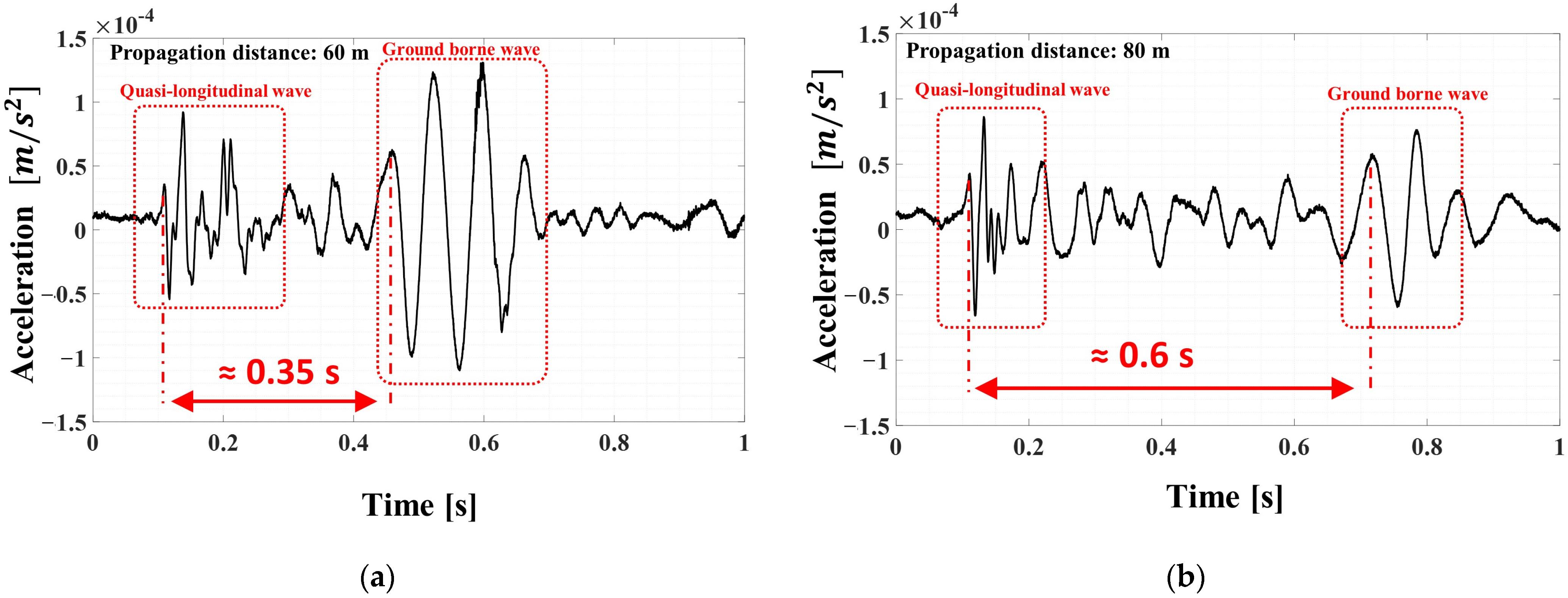
Additionally, when an impact is applied to the surface of the buried pipeline area, a ground-borne wave can also propagate [27,28], as shown in Figure 19a,b. The ground-borne wave refers to the wave that is generated when the impact energy is transmitted through the ground, and it is one of the noise sources that can cause errors in the source location. In particular, since the ground-borne wave is a type of transient signal that has a different propagation speed from the wave that propagates through the pipeline, it can introduce noise in the time-difference-of-arrival-based source location and needs to be filtered. Figure 19a shows the measured signal from the sensor position 60 m from the excavation site on the ground. As previously mentioned, quasi-longitudinal waves propagate at a speed of approximately 820 m/s and the ground-borne wave arrives approximately 0.35 s later. Because the propagation distance is 60 m, it can be determined that the propagation speed of the ground-borne wave is approximately 141 m/s. Figure 19b presents an excavation signal propagated 80 m, and it can be seen that the ground-borne wave arrives approximately 0.6 s later. Here, the time between the two wave groups was calculated based on the first peak, as shown in Figure 19a,b. Therefore, it can be estimated that the propagation speed of the ground-borne wave is approximately 114 m/s in this case. The ground-borne waves in the area where this experiment was conducted are known to propagate at approximately 200 m/s or less [29,30]. These ground-borne waves propagate in a transient shape with lower propagation speed compared to quasi-longitudinal waves, and they are known to cause source location errors due to their contribution as noise. However, the approach proposed in this study includes a step to confirm the similarity between these two types of signals, meaning that even in the presence of various forms of noise, including ground-borne waves, high accuracy in detecting the source location is possible.

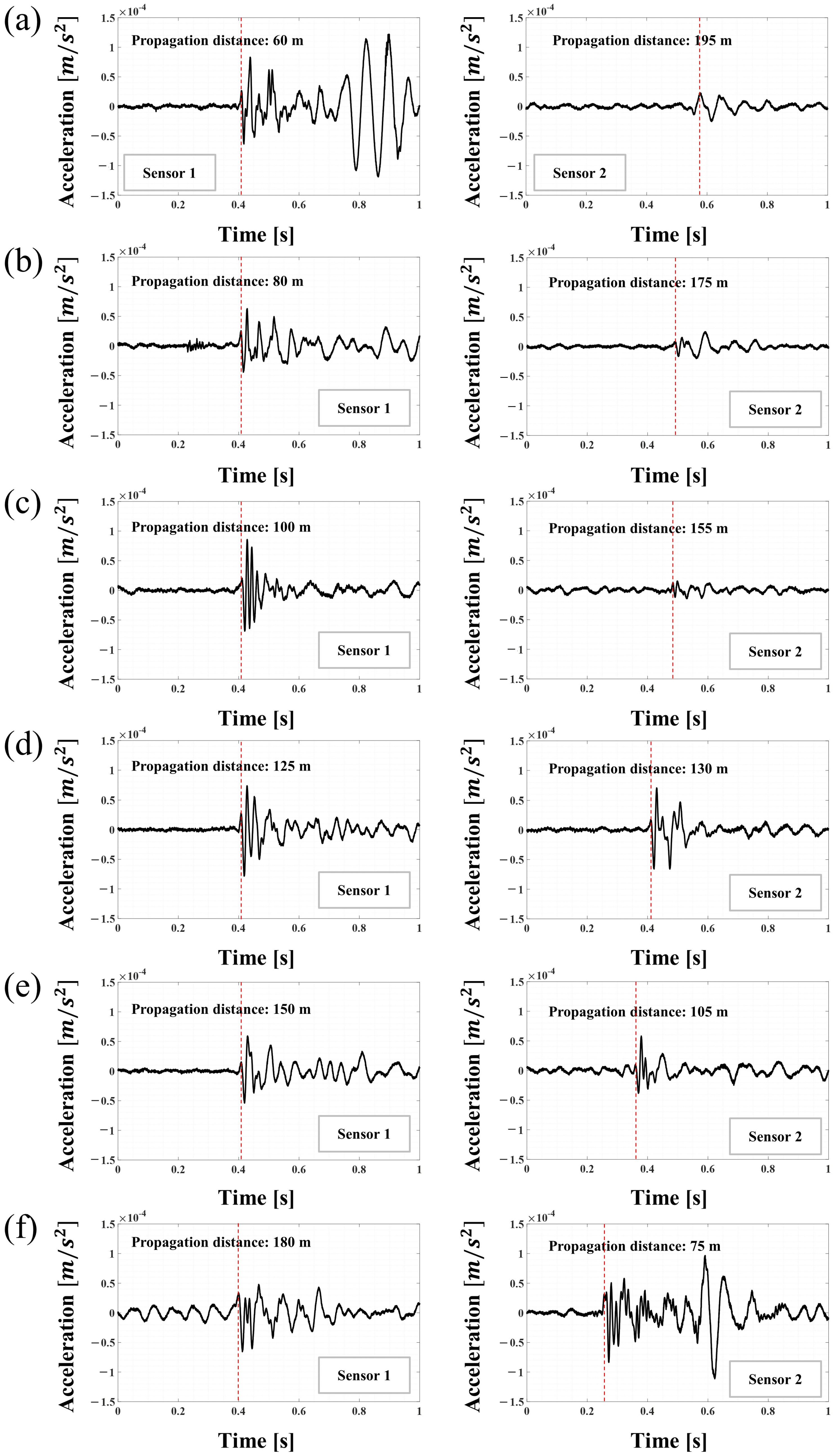
Figure 20a–f present signals obtained through excavation experiments conducted at various points. Here, the red dotted line indicates the location of the first peak of the quasi-longitudinal wave generated by TPI. Figure 20a shows the results of an excavation test at approximately 60 m from the sensor 1 position. In this case, the signal that reaches sensor 2 propagated a distance of approximately 195 m. As previously described, it can be confirmed that at a relatively short distance of 60 m, the ground-borne wave propagated together with the quasi-longitudinal wave at a speed of approximately 140 m/s. However, this cannot be confirmed at sensor 2, as the ground-borne wave was fully attenuated. Figure 20b through Figure 20f present signals obtained from excavations at distances of 80 m, 100 m, 125 m, 150 m, and 180 m from the position of sensor 1, respectively. Especially when observing the excavation signal at a location approximately 75 m from sensor 2 in Figure 20f, it can be observed that the ground-borne wave was measured concurrently, as shown in Figure 20a. As described above, these results suggest that the proposed $T{C}_{xy}\left(f,a\right)$ method contributes significantly to the selection of the optimal frequency bands for the source location. Since the signals were aligned with reference to the sensor 1 signal in Figure 20a–f, it can be observed that the time difference between the two signals gradually decreases. However, in Figure 20e,f, it can be observed that the sensor 2 signal arrives earlier because the distance from the impact to sensor 2 is shorter than the distance to sensor 1.

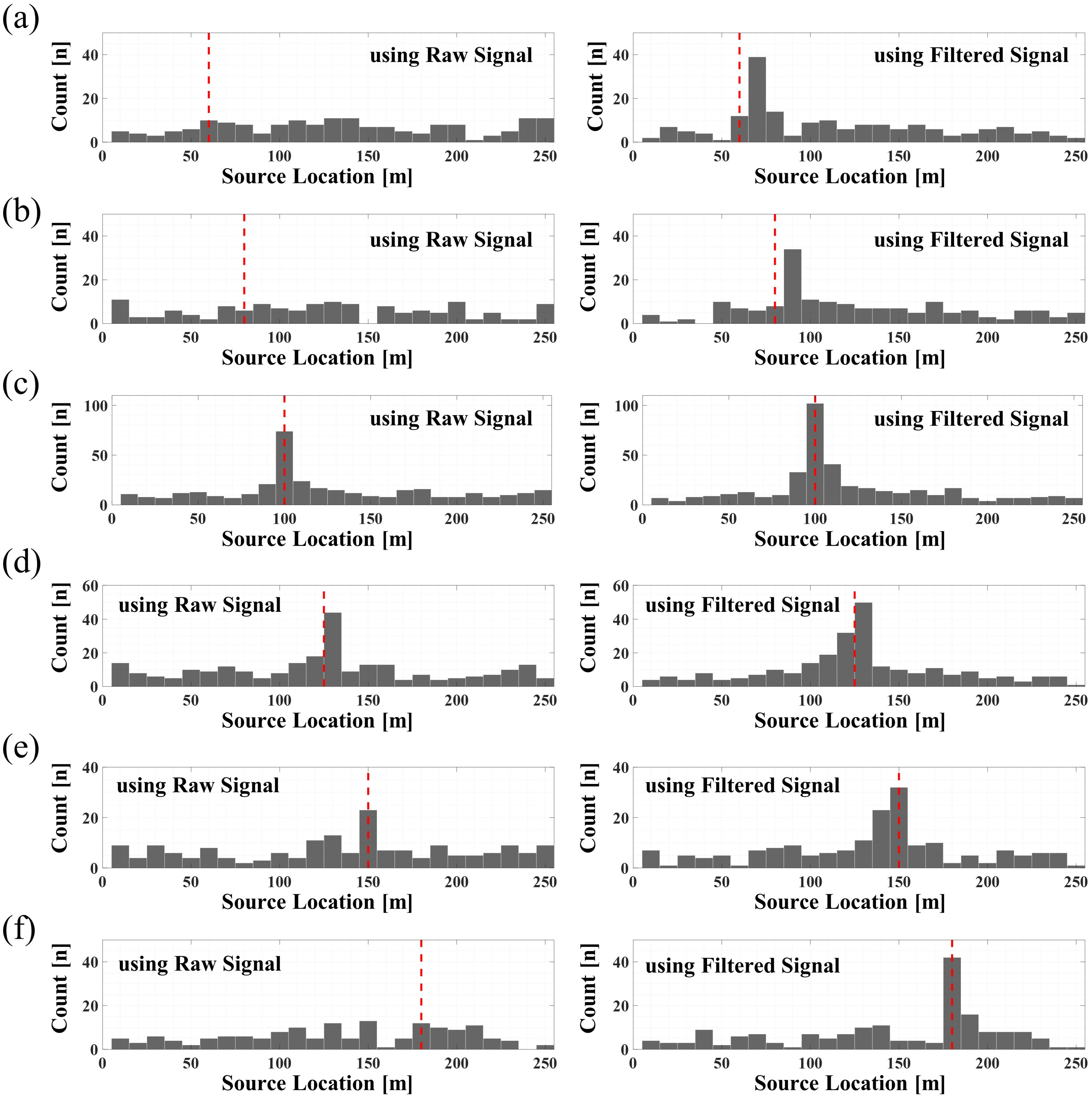
Figure 21a–f show the results after detecting excavation activity using raw and filtered signals. The actual excavation location is indicated by the red dashed line in all Figure 21a–f, with excavation activity carried out for approximately 120 s at each position. Figure 21a shows the source location results during excavation at a position of approximately 60 m. As a result, it was found that using the raw signal alone, it is not possible to detect excavation activity that can cause damage to the pipeline. However, by using the filtered signals obtained by the algorithm proposed in this study, excavation activity can be detected in the vicinity of 60 m. Similarly, Figure 21b–f present the verification results of the excavation activities performed at the 80 m, 100 m, 125 m, 150 m, and 180 m positions, respectively, using the proposed algorithm. The detection results at all positions indicate that the algorithm proposed in this study makes it possible to detect excavation activity that can cause pipeline damage. In particular, even in the presence of ground-borne waves and background noise in actual field conditions, it is possible to effectively pinpoint excavation activity by selecting the optimal frequency band for the impact wave. Therefore, the results of this study demonstrate the validity of detecting TPI that can directly cause impacts to buried pipelines, and this has significant utility in preventing pipeline failure accidents.

5. Conclusions

In this study, we proposed a novel algorithm that accurately identifies the location of TPI, which can cause direct damage to pipelines, for the early detection of pipeline failures. The algorithm utilizes FDK and a time-shift coherence function to evaluate the impact signals, enabling the effective design of a bandpass filter that improves the signal-to-noise ratio. Our experimental validation on large-diameter in-service waterworks pipelines demonstrated the algorithm’s effectiveness in detecting excavation activity at various locations, even in the presence of noise.

Furthermore, this study confirmed that an impact applied to the ground where a pipeline is buried not only propagates through the pipeline but also through ground-borne waves. Despite the presence of unwanted noise sources, including those generated by TPI as well as actual field noise, the proposed algorithm was experimentally validated to effectively detect excavation activity at various locations and remove the noise component, as demonstrated in the experimental results. The proposed approach allows for the detection of buried pipeline damage before a direct impact occurs, improving the safety of pipeline operations. The experimental results demonstrate the effectiveness of the algorithm in detecting excavation activity with a reasonable level of accuracy of less than 10 m, which corresponds to less than 5% of the monitoring range. These results provide a promising direction for further research on the early detection of pipeline failures due to impact damage caused, for instance, by TPI.

References

- Morgan, K.C. Managing Water Main Breaks: Field Guide; American Water Works Association: Denver, CO, USA, 2012. [Google Scholar]
- European Gas Incident Data Group. Gas Pipeline Incidents; 7th report, Report no. EGIG 08.TV-B.0502; European Gas Incident Data Group: Online, 2008. [Google Scholar]
- Goodfellow, G. Ukopa Pipeline Product; Report no. UKOPA/RP/21/001; UKOPA: Belper, UK, 2021. [Google Scholar]
- Li, S.; Peng, R.; Liu, Z. A surveillance system for urban buried pipeline subject to third-party threats based on fiber optic sensing and convolutional neural network. Struct. Health Monit. 2020, 20, 1704–1715. [Google Scholar] [CrossRef]
- Puust, R.; Kapelan, Z.; Savic, D.A.; Koppel, T. A review of methods for leakage management in pipe networks. Urban Water J. 2010, 7, 25–45. [Google Scholar] [CrossRef]
- Brainard, F.S. Leakage Problems and the Benefits off Leak Detection Programs. J.-Am. Water Work. Assoc. 1979, 71, 64–65. [Google Scholar] [CrossRef]
- Cole, E.S. Methods of Leak Detection: An Overview. J.-Am. Water Work. Assoc. 1979, 71, 73–75. [Google Scholar] [CrossRef]
- Fuchs, H.; Riehle, R. Ten years of experience with leak detection by acoustic signal analysis. Appl. Acoust. 1991, 33, 1–19. [Google Scholar] [CrossRef]
- Muggleton, J.; Brennan, M.; Linford, P. Axisymmetric wave propagation in fluid-filled pipes: Wavenumber measurements in in vacuo and buried pipes. J. Sound Vib. 2003, 270, 171–190. [Google Scholar] [CrossRef]
- Fuller, C.; Fahy, F. Characteristics of wave propagation and energy distributions in cylindrical elastic shells filled with fluid. J. Sound Vib. 1982, 81, 501–518. [Google Scholar] [CrossRef]
- Muggleton, J.; Yan, J. Wavenumber prediction and measurement of axisymmetric waves in buried fluid-filled pipes: Inclusion of shear coupling at a lubricated pipe/soil interface. J. Sound Vib. 2013, 332, 1216–1230. [Google Scholar] [CrossRef] [Green Version]
- Lee, Y.-S.; Yoon, D.-J. Improved Estimation of Leak Location of Pipelines Using Frequency Band Variation. J. Korean Soc. Nondestruct. Test. 2014, 34, 44–52. [Google Scholar] [CrossRef]
- Behari, N.; Sheriff, M.Z.; Rahman, M.A.; Nounou, M.; Hassan, I.; Nounou, H. Chronic leak detection for single and multiphase flow: A critical review on onshore and offshore subsea and arctic conditions. J. Nat. Gas Sci. Eng. 2020, 81, 103460. [Google Scholar] [CrossRef]
- Shin, S.-M.; Suh, J.-H.; Im, J.-S.; Kim, S.B.; Yoo, H.-R. Development of Third-Party Damage Monitoring System for Natural Gas Pipeline. KSME Int. J. 2003, 17, 1423–1430. [Google Scholar] [CrossRef]
- Park, C.-S.; Lee, S.-H.; Yoon, D.-J. Enhancing Impact Localization from Fluid-Pipe Coupled Vibration under Noisy Environment. Appl. Sci. 2021, 11, 4197. [Google Scholar] [CrossRef]
- Bjorklund, S.; Ljung, L. A review of time-delay estimation techniques. In Proceedings of the 42nd IEEE International Conference on Decision and Control (IEEE Cat. No.03CH37475), Maui, HI, USA, 9–12 December 2003; Volume 3, pp. 2502–2507. [Google Scholar] [CrossRef] [Green Version]
- Lee, Y.-S. Effects of windowing filters in leak locating for buried water-filled cast iron pipes. J. Mech. Sci. Technol. 2009, 23, 401–408. [Google Scholar] [CrossRef]
- Hannan, E.J.; Thomson, P.J. Estimating group delay. Biometrika 1973, 60, 241–253. [Google Scholar] [CrossRef]
- Roth, P.R. Effective measurements using digital signal analysis. IEEE Spectr. 1971, 8, 62–70. [Google Scholar] [CrossRef]
- Carter, G.; Nuttall, A.; Cable, P. The smoothed coherence transform. Proc. IEEE 1973, 61, 1497–1498. [Google Scholar] [CrossRef]
- Lee, S.-H.; Park, C.-S.; Yoon, D.-J. Experimental Verification of Impact Damage Detection in Long Range Buried Water Supply Pipeline. J. Korean Soc. Nondestruct. Test. 2020, 40, 241–250. [Google Scholar] [CrossRef]
- Randall, R.; Tech, B. Frequency analysis (bruel & kjaer). In Preventative Maintenance Program Handbook (IRD Mechanalysis); Estate Ltd.: Hong Kong, China, 1987. [Google Scholar]
- Almeida, F.C.; Brennan, M.J.; Joseph, P.F.; Dray, S.; Whitfield, S.; Paschoalini, A.T. Towards an in-situ measurement of wave velocity in buried plastic water distribution pipes for the purposes of leak location. J. Sound Vib. 2015, 359, 40–55. [Google Scholar] [CrossRef]
- Dwyer, R.F. A technique for improving detection and estimation of signals contaminated by under ice noise. J. Acoust. Soc. Am. 1983, 74, 124–130. [Google Scholar] [CrossRef]
- Dwyer, R. Use of the kurtosis statistic in the frequency domain as an aid in detecting random signals. IEEE J. Ocean. Eng. 1984, 9, 85–92. [Google Scholar] [CrossRef] [Green Version]
- Ottonello, C.; Pagnan, S. Modified frequency domain kurtosis for signal processing. Electron. Lett. 1994, 30, 1117–1118. [Google Scholar] [CrossRef]
- Foti, S.; Hollender, F.; Garofalo, F.; Albarello, D.; Asten, M.; Bard, P.-Y.; Comina, C.; Cornou, C.; Cox, B.; Di Giulio, G.; et al. Guidelines for the good practice of surface wave analysis: A product of the InterPACIFIC project. Bull. Earthq. Eng. 2017, 16, 2367–2420. [Google Scholar] [CrossRef]
- Colaço, A.; Ferreira, M.A.; Costa, P.A. Empirical, Experimental and Numerical Prediction of Ground-Borne Vibrations Induced by Impact Pile Driving. Vibration 2022, 5, 80–95. [Google Scholar] [CrossRef]
- Astrauskas, T.; Grubliauskas, R.; Januševičius, T. Investigation and Evaluation of Speed Table Influence on Road Traffic Induced Ground Borne Vibration. In Environmental Engineering, Proceedings of the International Conference on Environmental Engineering; Department of Construction Economics & Property, Vilnius Gediminas Technical University: Vilnius, Lithuania, 2017; Volume 10, pp. 1–7. [Google Scholar] [CrossRef]
- Graff, K.F. Wave Motion in Elastic Solids; Courier Corporation: Chelmsford, MA, USA, 2012. [Google Scholar]
Figure 1.
Source location in a buried pipeline with two sensors.
Figure 2.
Dispersion curve of a quasi-longitudinal wave depending on the diameter.
Figure 3.
Dispersion curve of a quasi-longitudinal wave depending on the materials.
Figure 4.
Virtual measurement signal: (a) virtual measurement signal x(t) and (b) virtual measurement signal y(t).
Figure 5.
Frequency response calculated by the virtual measurement signal: (a) frequency response calculated by virtual measurement signal x(t) and (b) frequency response calculated by virtual measurement signal y(t).
Figure 6.
Coherence results calculated using transient signals.
Figure 7.
Results of FDK: (a) FDK using virtual measurement signal x(t) and (b) FDK using virtual measurement signal y(t).
Figure 8.
Results of time-shift coherence using transient signals.
Figure 9.
Time signal obtained after the optimal bandpass filter process: (a) using signal x(t) and (b) using signal y(t).
Figure 10.
Cross-correlation using filtered signals.
Figure 11.
Impact-damage detection algorithms.
Figure 12.
Schematics for the experiments: (a) pipeline layout on map and (b) backhoe excavation.
Figure 13.
Illustration for the experimental scenario.
Figure 14.
Time-domain signals obtained from each sensor: (a) sensor 1 and (b) sensor 2.
Figure 15.
FDK obtained from each sensor: (a) sensor 1 and (b) sensor 2.
Figure 16.
Time-shift coherence results using measured signals.
Figure 17.
Time-domain signal obtained after the optimal bandpass filter process: (a) sensor 1 and (b) sensor 2.
Figure 18.
Cross-correlation results using the filtered signals.
Figure 19.
Time-domain signals obtained from each sensor including a ground-borne wave: (a) propagation distance of 60 m and (b) propagation distance of 80 m.
Figure 20.
Excavation signals obtained at various points: (a) results of the excavation test at 60 m, (b) results of the excavation test at 80 m, (c) results of the excavation test at 100 m, (d) results of the excavation test at 120 m, (e) results of the excavation test at 150 m, and (f) results of the excavation test at 180 m.
Figure 21.
Results of source location comparisons of raw signal and filtered signal: (a) results of the excavation test at 60 m, (b) results of the excavation test at 80 m, (c) results of the excavation test at 100 m, (d) results of the excavation test at 120 m, (e) results of the excavation test at 150 m, and (f) results of the excavation test at 180 m.
Disclaimer/Publisher’s Note: The statements, opinions and data contained in all publications are solely those of the individual author(s) and contributor(s) and not of MDPI and/or the editor(s). MDPI and/or the editor(s) disclaim responsibility for any injury to people or property resulting from any ideas, methods, instructions or products referred to in the content. |
© 2023 by the authors. Licensee MDPI, Basel, Switzerland. This article is an open access article distributed under the terms and conditions of the Creative Commons Attribution (CC BY) license (https://creativecommons.org/licenses/by/4.0/).
Share and Cite
MDPI and ACS Style
Lee, S.-H.; Park, C.-S.; Yoon, D.-J. Early Detection and Identification of Damage in In-Service Waterworks Pipelines Based on Frequency-Domain Kurtosis and Time-Shift Coherence. Water 2023, 15, 1189. https://doi.org/10.3390/w15061189
AMA Style
Lee S-H, Park C-S, Yoon D-J. Early Detection and Identification of Damage in In-Service Waterworks Pipelines Based on Frequency-Domain Kurtosis and Time-Shift Coherence. Water. 2023; 15(6):1189. https://doi.org/10.3390/w15061189
Chicago/Turabian StyleLee, Sun-Ho, Choon-Su Park, and Dong-Jin Yoon. 2023. "Early Detection and Identification of Damage in In-Service Waterworks Pipelines Based on Frequency-Domain Kurtosis and Time-Shift Coherence" Water 15, no. 6: 1189. https://doi.org/10.3390/w15061189
Note that from the first issue of 2016, this journal uses article numbers instead of page numbers. See further details here.