Discharge Coefficients of a Specific Vertical Slot Fishway Geometry—New Fitting Parameters

Abstract

Fishways are essential hydraulic structures to ensure the migration of fish and other aquatic organisms in the area of cross structures in river systems. In this context, the present study focuses on vertical slot fishways with specific geometries and their discharge coefficients. A comprehensive data analysis was performed, aiming on the development of new fitting parameters in conjunction with their respective approaches for practical design procedures. In addition, validity ranges and parameter dependencies were defined. Using the new fitting equations, it is possible to determine accurate discharge coefficients to design functional strutures for a defined validity range. Results show that discharge coefficients are highly dependent on the basin geometry. Comparing newly developed fitting parameters have shown that investigated fitting equations can be used to determine discharge coefficients. However, it should be noted that newly developed fittings can only be applied in practice for the defined range of validity for investigated exemplary geometries.

1. Introduction

During the last decades, fish migration becomes a mandatory criteria in the field of water policy and water management concerning the treatment of water, established by the European Water Framework Directive [1], and various design guidelines were developed. The [1] specifically defines criteria for maintaining or restoring a water body into a “good condition”. This condition basically includes three major components: (1) biological, (2) hydromorphological, and (3) chemical-physical components. To solve various problems related to the fish passability and river continuity, it may require implementation measures, such as a complete deconstruction of existing cross structures or the construction of replacement structures, like split structures, naturally designed bypass channels, or technical fishways. Fishways are hydraulic structures which must be designed concerning several aspects, like for example feasibility of fish migration, energy dissipation, stability, general hydraulic parameters, or resulting upstream heads. Generally, German guidelines dictate that the passability must be guaranteed for approximately 300 days a year (between $Q_{30}$ and $Q_{330}$) and consequently a detailed knowledge of existing statistical duration periods is necessary. Thereby, $Q_{30}$ represents the averaged statistical discharge which will be undercut only at 30 days a year; and analogously $Q_{330}$ will be exceeded only 35 days a year [2].

Basically, fishways can be classified into (1) technical or (2) nature-based structures. On one hand, technical fish passes include configurations with basin structures, such as single or double slot passes, round basin passes, or other technical solutions. On the other hand, nature-oriented structures are divided into rough channels with included bed roughness (not fixed to the bed), rough channels with individually placed boulders, and rough channels with formed basin structures, also called crossbar block ramps. Technical fishways are often used where, for example, technical boundary conditions, space availability, or economic conditions do not allow large structures. Hence, technical fishways can represent an adequate solution to guarantee fish migration and to conquer large river bottom steps [3].

The present study mainly focuses on technical fish passes—so called vertical slot fishways (VSF). These structures can be constructed directly on or in the cross structure. VSFs come with a high cost-efficiency and a space-saving design, which makes them suitable for existing migration barriers with limited space.

Slot passes are constructed by installing vertical walls on a uniformly sloped channel (see Figure 1). These walls form a predefined number of basins which are connected via vertical slots. Aquatic organisms can migrate through these vertical slots from basin to basin. For near-bottom migration also rough base material can be included within the basins. The hydraulic design of a VSF depends on the given design fish and consequently slot widths, basins lengths, and discharges can be calculated. For instance, the flow within the basins can be modified by varying slot geometries, guiding elements, or baffled blocks on the side walls. Consequently, areas of high flow velocities in the slots and resting zones in the basins can be generated, which also influences tailwater and headwater next to the slots [2,3].

To guarantee the functionality of a VSF, an accurate design is essential and design parameters must be developed or adapted. Therefore, various discharge equations are available and discharge coefficients can be calculated. The objective of the present paper is to develop new fittings (empirically determined coefficients ${\alpha }_1$, ${\alpha }_2$, $\beta$) for a specific geometry of VSF. With these newly fitted parameters, discharge coefficients can be determined with high accuracy. Furthermore, dependencies and validity ranges are determined via comparative analysis of resulting discharge coefficients. The basis for the performed data analysis and final determination of the used fitting equations are numerous laboratory measurement campaigns, which are summarized in this paper.

2. State-of-the-Art

Numerous scientific and non-scientific contributions exist at national and international levels with various contexts on the flow behavior of fishways, such as VSFs. Usually, developed design guidelines are based on data collected from scaled experimental models or numerical 3D-CFD simulations. Research investigations at Karlsruhe Institute of Technology (KIT), the Federal Waterways Engineering and Research Institute (BAW), and the author’s past and current hydraulics laboratories carried out numerous VSF model tests with various slot angles and positions of guiding elements [4]. Flow patterns, flow velocities, water level differences, and resulting discharges were also taken into account for the hydraulic design of VSF. Data from numerous measurement campaigns were included for proper dimensioning and analysis procedures.

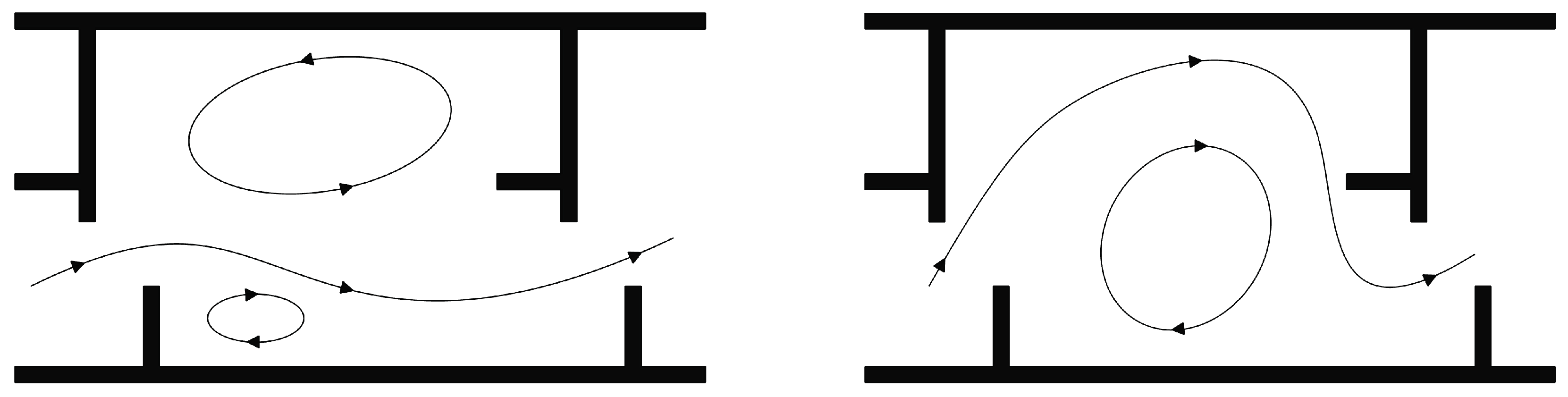
Based on numerous studies, [5] found that two different flow patterns can be generated in the basins of slot passes (see Figure 2). The flow-stable current pattern (flow pattern 1) is a kind of short-circuit flow from slot to slot, as well as two vortices each at the edge of the main flow within the basins. In contrast, for the flow-dissipating current pattern (flow pattern 2) the main flow is majorly deflected, whereby the main current hits the downstream vertical wall and energy dissipation occurs [2,6].Several studies have found that the formation of flow patterns is influenced by the slope, flow conditions and $W/L$-ratio (W = basin width, L = basin length, measured from half of one wall to half of the next wall within a basin) [5,7,8,9,10]. Exemplary, flow pattern 1 occurs for the $W{L}^{-1}$ > 0.77 and pattern 2 for $W{L}^{-1}$ < 0.77 [8]. In this context, [11] performed numerical simulations with a 3D computational fluid dynamics model and found that due to various parameters, such as the mean flow and turbulence characteristics in VSF, fish experiments should be performed next to flow experiments.

Flow conditions in VSF basins will be mostly turbulent [12] and the degree of turbulences might influence the fish behaviour and their climb capability. Additionally, the flow conditions can be superimposed by irregular fluctuations., caused by large eddies and alternating motions. The eddies create an intense pulse change in the flow through the basin and consequently, turbulences cannot be clearly predicted and described. A specific feature of turbulent flows is the fluctuating and non-uniform velocity field in space and time [13]. Ref. [9] mentioned that the flow in VSF is completely turbulent and various studies proof that the variations in flow, both in terms of flow velocities and eddy formation, are very different from statistical means [5,9,14].

Next to flow patterns, flow velocities were often investigated to identify hydraulic design criteria. Ref. [15] performed experimental model tests to investigate hydraulic phenomena of slot passes. Based on the results, Ref. [15] determined that the maximum flow velocity $v_{\max }$ in the slot can be approximately calculated using the following typical equation:

$$v_{\max }=\sqrt{2g\Delta h}$$

(1)

where: g = acceleration due to gravity, $\Delta h=LS$ = water level difference between two basins, L = basin length, S = slope.

Hence, the decisive parameter for determining the maximum flow velocity $v_{\max }$ is the water level difference $\Delta h$ of two adjacent basins. Theoretically, the water level in the slot pass basin is assumed to be horizontal and thus can be determined by the bottom slope difference $\Delta z$, which equals $\Delta h$ [15,16]. The development of the water level depends basically on the slope, the slot width, and the basin geometry [2]. However, the actual water surface is three-dimensional and is not constant over the width or length in non-uniform. flow conditions [15,16,17] with $\Delta h\ne \Delta z$. It should be noted, that uniformity on VSF is not meant to be the normal flow depth; furthermore, it describes a situation where the flow characteristics are not changing from basin to basin while the flow in each basin itself is non-uniform due to backwater and fluctuation effects.

Another decisive design parameter is the acceptable minimum water level in the basin, which depends on the respective fish species. This water level can be calculated via the discharge. In practice, two analytical approaches [(a), (b)] are commonly used to determine the discharge Q in vertical slot passes [2,6].

(a) The first approach is based on the flow through a slot as a channel constriction without flow transition according to Venturi or Poleni [18,19]:

$$Q=\frac{2}{3}{C}_{d,1}{b}_0\sqrt{2g}{h}_1^{1.5}$$

(2)

where: $C_{d,1}$ = discharge coefficient, $b_0$ = slot width, $h_1$ = headwater level.

Herein, the discharge coefficient $C_d$ can be approximately calculated depending on the headwater level $h_1$ and tailwater level $h_2$ [2,3,19]:

$$C_d={\alpha }_1{\left[1-{\left(\frac{h_2}{h_1}\right)}^{\beta }\right]}^{{\alpha }_2}$$

(3)

where: ${\alpha }_1,{\alpha }_2,\beta$ = empirically determined coefficients.

If backwater influences can be neglected, the discharge coefficient must reach a constant value. This can be controlled by the parameter $\beta$ [2,3]. In this case, the coefficient $\beta$ can be assumed with a value of 4.5, and coefficients ${\alpha }_1$ and ${\alpha }_2$ can be separately defined for flow-stable and flow-dissipating conditions [2,20]. The discharge coefficients according to [2,20] can be described as a function of the flow pattern for a validity range 0.5 < $h_2{h}_1^{-1}$ < 0.99 and $h_2$ > $2b_0$.

Flow-stable conditions:

$$C_{d,1}=0.48·{\left[1-{\left(\frac{h_2}{h_1}\right)}^{4.5}\right]}^{0.60}$$

(4)

Flow-dissipating conditions:

$$C_{d,1}=0.59·{[1-{\left(\frac{h_2}{h_1}\right)}^{4.5}]}^{0.48}$$

(5)

In addition, [20] established a mean fitting for the same validity range with $\beta$ = 4.50, ${\alpha }_1$ = 0.53, ${\alpha }_2$ = 0.52. In conjunction with the empirical approach according to Villemonte [21] for a discharge coefficient for submerged weirs, Equation (3) can be used. Ref. [21] defines different values for $\beta$ depending on weir construction. Coefficient ${\alpha }_2$ is assumed to be 0.385 for submerged weirs. ${\alpha }_1$ is set as a constant approximation in this context. Various investigations show that this approach (Equation (3)) can also be used to determine several discharge coefficients of fishways with slots and notches (e.g., VSF) [18,19,20]. The coefficient $\beta$ can be assumed to be 1.5 according to [18,19,21]. However, following [19], it is necessary to estimate the parameters for ${\alpha }_1$ and ${\alpha }_2$ to obtain an optimal fit for different geometries. Discharge coefficients can be determined in accordance with [18] for different guiding elements:

Basic guide element:

$$C_{d,1}=0.84·{\left[1-{\left(\frac{h_2}{h_1}\right)}^{1.5}\right]}^{0.43}$$

(6)

Hook-shaped guide element:

$$C_{d,1}=0.72·{[1-{\left(\frac{h_2}{h_1}\right)}^{1.5}]}^{0.33}$$

(7)

Furthermore, Ref. [18] defined a further discharge coefficient $C_{d,1}$ with $\beta$ = 1.50, ${\alpha }_1$ = 0.57 and ${\alpha }_2$ = 0.40. For discharge coefficients listed above according to [18], the coefficient of determination is given as $R^2$ = 0.81 to 0.96. [3] performed an additonal fitting with the results $\beta$ = 2.50, ${\alpha }_1$ = 0.72, ${\alpha }_2$ = 0.47 ($R^2$ = 0.97).

The mentioned design approach according to the Venturi equation has also been confirmed for submerged discharges by [20]. It was observed, that the flow beam entering the basin does not flow through the basin at full width [2,20]. Various studies showed the applicability of the design approach based on Venturi or Poleni, although discharge coefficients only represent an empirical approximation and can be transferred only to limited geometrical variations (basin sizes, slot widths, guide elements, baffle blocks) of the slot pass [3].

(b) The second approach is based on the Torricelli equation, with a maximum flow velocity $v_{\max }$ (see Equation (1)):

$$Q=C_{d,2}{A}_d\sqrt{2g\Delta h}$$

(8)

where: $C_{d,2}$ = discharge coefficient, $A_d=b_{0}h$ = flow area, h = flow depth, $\sqrt{2g\Delta h}=v_{\max }$ = maximum flow velocity.

This design approach has been further developed for several years and is a central approach for determining discharge values and ensuring a minimum water level [15,22]. According to [18], assuming that Equation (8) becomes Equation (2) for free flow conditions, discharge coefficients $C_{d,2}$ may also be calculated approximately via Equation (3). Therefore, Ref. [18] present the following values for $C_{d,2}$: $\beta$ = 1.50, ${\alpha }_1$ = 0.54 and ${\alpha }_2$ = $-0.20$ ($R^2$ = 0.45). Based on [4] parameters can be assumed as $\beta$ = 2.50, ${\alpha }_1$ = 0.68, ${\alpha }_2$ = $-0.07$ ($R^2$ = 0.41). However, it appears that the adjustment of discharge coefficients for in-situ measurements and comparative values show significantly deviated results [18].

In addition to the analytical approaches listed for determining discharges in VSP, Refs. [15,17] describe the use of dimensionless discharges $Q^{*}=Q{\left(gS{b}_0^5\right)}^{-0.5}$ and their relationships with average flow depth and slot geometry $y_0{b}_0^{-1}$. This leads to the following linear relationship: $Q^{*}=A\left(y_0{b}_0^{-1}\right)+B$ where A, B are the coefficients depending on the fishway geometry [5]. Besides [16], other studies have been carried out on dimensionless discharge. Ref. [5] further developed the equation and established additional relationships [18].

3. Experimental Model Data

Experimental models are frequently used to investigate geometrical parameter influences for VSF design purposes. Resulting data can be used to develop empirical approaches, especially for discharge coefficients. Several scaled model campaigns were performed and scale effects must be taken into account to guarantee adequate results and to allow the transfer to prototype scales. Geometrical boundary conditions are chosen based on existing scientific investigations, available design guidelines, and prototype experiences. As a result, large amounts of datasets are available in the literature.

Table 1. Overview of experimental parameters from different datasets.

	Design	W	L	${\mathit{b}}_0$	${\mathit{WL}}^{-1}$	${\mathit{Wb}}_0^{-1}$	${\mathit{Lb}}_0^{-1}$	S	Q	${\mathit{l}}_{\mathit{g}}$	${\mathit{l}}_{\mathit{g}}{\mathit{b}}_0^{-1}$	Typ of Guide Element
Mohlfeld and Oertel (2021) [3]	3	0.8	1.021	0.119	0.78	6.72	8.58	0.025; 0.050	0.016; 0.024; 0.032	0.190	1.60	linear
	4	0.8	1.021	0.119	0.78	6.72	8.58			0.178	1.50	linear
	5	0.8	1.021	0.119	0.78	6.72	8.58			0.178	1.50	bevelled
	6	0.8	1.021	0.119	0.78	6.72	8.58			0.178	1.50	spline
	7	0.8	1.021	0.119	0.78	6.72	8.58			0.178	1.50	quadrant
BAW (2019) [23]	3	0.8	1.01	0.120	0.79	6.67	8.42	0.028; 0.039;	0.010 to 0.035			linear
	3	0.79	1.02	0.122	0.77	6.43	8.36	0.050; 0.028				linear
Klein and Oertel (2018) [25]	3	0.8	1.021	0.119	0.78	6.72	8.58			0.190	1.60	linear
	3.67	0.8	1.021	0.119	0.78	6.72	8.58			0.190	1.60	linear
	4	0.8	1.021	0.119	0.78	6.72	8.58	0.025; 0.050	0.008 to 0.044	0.178	1.50	linear
	5	0.8	1.021	0.119	0.78	6.72	8.58			0.178	1.50	bevelled
	6	0.8	1.021	0.119	0.78	6.72	8.58			0.178	1.50	spline
	7	0.8	1.021	0.119	0.78	6.72	8.58			0.178	1.50	quadrant
Klein and Oertel (2017) [6]	37	0.8	1.021	0.119	0.78	6.72	8.58		0.005 to 0.056	0.190	1.60	linear
	52	0.8	1.021	0.119	0.78	6.72	8.58	0.050		0.190	1.60	linear
	67	0.8	1.021	0.119	0.78	6.72	8.58			0.190	1.60	linear
Krüger et al. (2010) [20]	1	3.3	4.5	0.45	0.73	7.33	10.00	0.056	0.769; 0.933; 1.101			none
Bermúdez et al. (2010) [7]	2	0.3	0.38	0.168; 0.084; 0.043	0.80	1.79; 3.58; 7.16	2.24; 4.47; 8.94	0.050	0.0009 to 0.0270			none
	2	0.3	0.75	0.168; 0.084	0.40	1.79; 3.58	4.47; 8.94					none
	2	0.3	1.50	0.168	0.20	1.79	8.94					none
	2	0.3	2.25	0.168	0.13	1.79	13.42					none
	2	0.3	0.28	0.126	1.07	2.39	2.24					none
	2	0.3	0.57	0.126; 0.043	0.53	2.39; 7.16	4.47; 13.42					none
	2	0.3	1.13	0.126; 0.084	0.27	2.39; 3.58	8.94; 13.42					none
	2	0.3	1.70	0.126	0.18	2.39	13.34					none
	2	0.3	0.19	0.084; 0.043	1.60	3.58; 7.16	2.24; 4.47					none
	2	0.3	0.095	0.043	3.20	7.16	2.24					none
Puertas et al. (2004) [16]	1	0.99	1.21	0.16	0.82	6.19	7.58	0.0570; 0.1005	0.0159 to 0.1250	0.243	1.52	linear
	2	0.99	1.21	0.15	0.82	6.60	8.09					none
Rajaratnam et al. (1992) [17]	1	0.458	0.572	0.057	0.80	8.00	10.00	0.10	0.0009 to 0.026	0.086	1.50	bevelled
	6	0.305	0.381	0.043	0.80	7.16	8.94	0.057; 0.10				none
	8	0.305	0.191	0.043	1.60	7.16	4.47	0.10; 0.149				none
	9	0.153	0.191	0.043	0.80	3.58	4.47	0.10; 0.149				none
	11	0.305	0.572	0.043	0.53	7.16	13.42	0.050; 0.10				none
	14	0.305	0.381	0.043	0.80	7.16	8.94	0.050; 0.10; 0.148		0.086	2.00	linear
	15	0.305	0.381	0.043	0.80	7.16	8.94	0.050; 0.10; 0.148		0.086	2.00	linear
	16	0.305	0.381	0.046	0.80	6.65	8.31	0.050; 0.10		0.092	2.00	linear
	17	0.305	0.381	0.038	0.80	8.00	10.00	0.10; 0.150		0.057	1.50	round
	18	0.305	0.381	0.038	0.80	8.00	10.00	0.10; 0.150		0.057	1.50	spline

summarizes many specifications and corresponding boundary conditions of previously performed investigations. The datasets listed have been made available and can be viewed in more detail in relevant literature. Dataset [23] will be evaluated and presented in [24]. A closer look at Table 1 shows that there are some differences in the generated geometries of the datasets. Nevertheless, these datasets are listed and considered in the evaluation to get an overview of the dependencies of the different geometric parameters and to demonstrate the importance of adhering to the validity ranges.

Generally, the principle of experimental model runs in hydraulics laboratories is identical for worldwide experiments, while size and discharge limitations directly influence resulting model scales. Water is being circulated in a pump and pipe system and finally guided into a flume (for VSF investigations a tilting flume was chosen), in which the slot pass geometry was installed. The length of the model and consequently the amount of basins shall guarantee a quasi-uniform flow from basin to basin (equal conditions in all basins). Additionally, e.g., tailwater effects can be analyzed. The main design parameters are flow depths and flow velocities; hence, Ultrasonic sensors (USS) and Acoustic Doppler Velocimetry (ADV) probes can be used for measurements. If focussing on areal measurements, instead of point measurements, automated positioning systems allow a reproducible probe placement. Focusing on Equations (2) and (8) it becomes clear that the benefit of a hydraulics laboratory is the detailed knowledge about the provided discharge Q (measured via magnetic inductive flow meter, MID). With collected flow depths and discharges, discharge coefficients $C_d$ can be finally calculated.

4. Results and Discussion

4.1. General

For further consideration of the measurement data used, measurement campaigns are compared and new fitting curves are developed within this study. Thereby, literature data from Table 1 is used for data comparison and further investigations. For the comparability of different data from various measurement campaigns, geometric parameters should be clearly defined. Hence, it was decided to calculate headwater depths $h_1$ and tailwater depths $h_2$ of the individual basins from the area-averaged mean flow depth $h_m$ and the water level difference $\Delta h$ of the two successive basins to estimate $h_{1,m}$ and $h_{2,m}$ [3]:

$$h_{1,m}=h_m+0.50\Delta h$$

$$h_{2,m}=h_m-0.50\Delta h$$

where: $\Delta h=LS=\Delta z$. These calculated headwater and tailwater depths are often used in the literature to determine discharge coefficients [7,18,19]. It should be noted that the water level in the slot pass is assumed to be horizontal and the general flow condition is quasi-uniform from basin to basin (neglecting fluctuation and tailwater effects).

To compare various data from the literature, discharge coefficients $C_d$ are determined using the equations explained in Chapter Section 2 while considering $h_{2,m}{h}_{1,m}^{-1}$ as $h_2{h}_1^{-1}$.

4.2. Discharge Coefficients in Accordance with Poleni

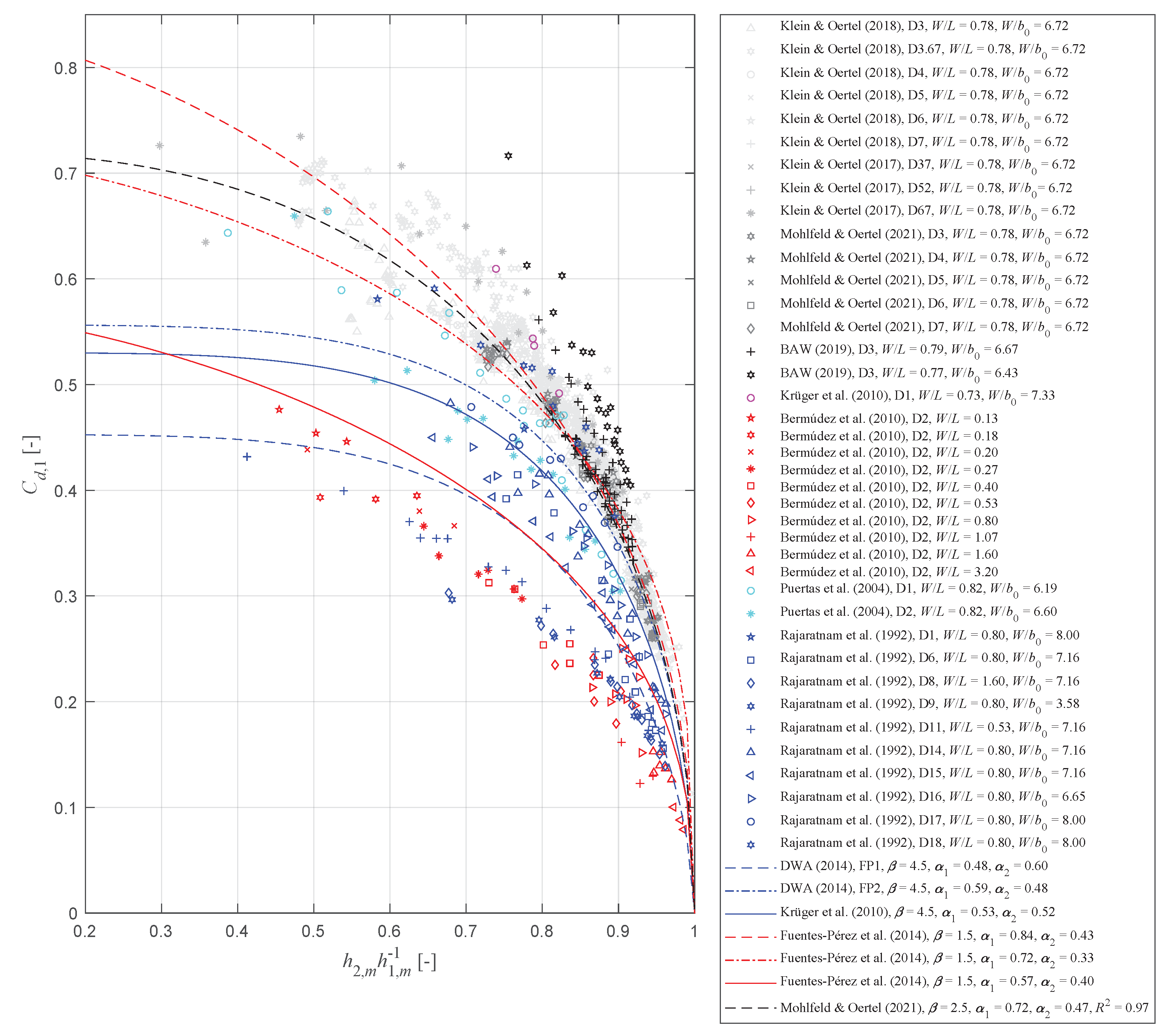
Figure 3 shows resulting discharge coefficients $C_{d,1}$, calculated using Equation (2) as a function of $h_{1,m}$ and Q for all data from the literature.

It can be seen that several fitting approaches exist for various VSF configurations with more or less good agreement with the provided datasets. In Figure 3 black and gray data points represent new experimental model results. It can be found that, only one equation can be used for several geometrical model variations (bottom slope, offset angle, guide element, etc.) to estimate discharge coefficients $C_d$.

For $h_{2,m}{h}_{1,m}^{-1}$ > 0.8 only minor deviations exist between the established fitting curves; such as for the flow-dissipating discharge (Equation (5)) and the equations of [18] (Equations (6) and (7)). But especially some of the latest fitting equations (e.g., Equation (4) of [2,20]) significantly deviate from new collected data, since narrow or wide basins with particularly small slot openings were used in the past [3]. Furthermore, it can be seen that for smaller $h_{2,m}{h}_{1,m}^{-1}$, there are larger deviations between the fitting curves. This demonstrates that for smaller $h_{2,m}{h}_{1,m}^{-1}$ the influences on the discharge coefficients become significantly greater, and therefore the geometric boundary conditions and compliance with the validity ranges play a greater role.

Figure 3. Discharge coefficients and existing fitting equations according to Equation (3) based on Poleni (Equation (2)) [2,3,6,7,16,17,18,20,23,25].

Figure 3. Discharge coefficients and existing fitting equations according to Equation (3) based on Poleni (Equation (2)) [2,3,6,7,16,17,18,20,23,25].

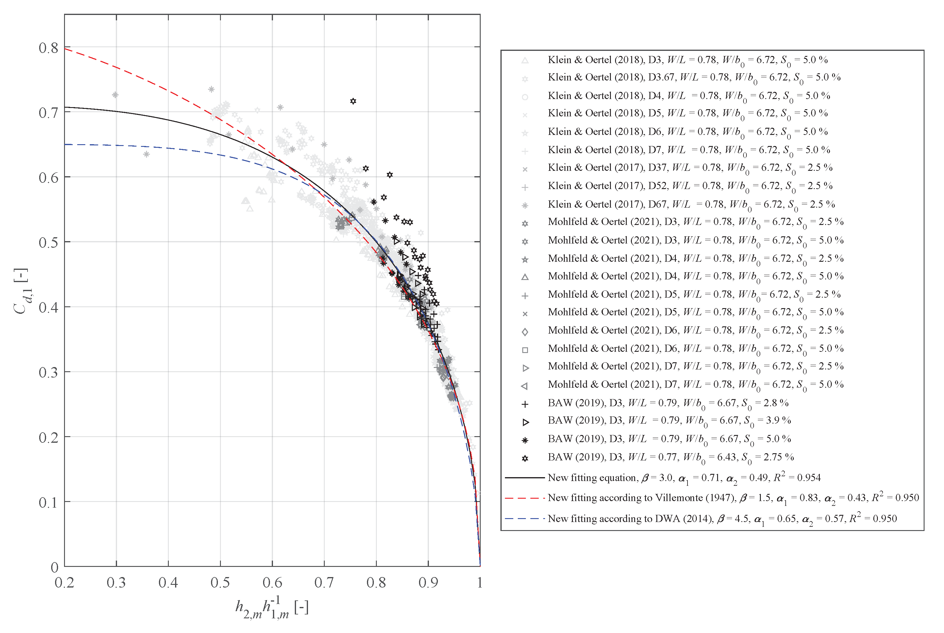
For further investigations and practical design approaches, new fitting parameters were developed using the datasets of [3,6,23,25], since similar boundary conditions were used within these measurement campaigns and the VSFs were gently sloped. These fittings are used for the calculation of discharge coefficients according to Equation (3) for discharge calculations via Equation (2). In order to assess the state of the art, different fitting curves were generated with $\beta$ = 1.5 according to [18,19,21] and $\beta$ = 4.5 according to [2,20]. In addition, the best fitting with $\beta$ = 3.0 was developed for the data. The forementioned fitting can be described by the following equation:

$$C_{d,1,\mathrm{calc}}=0.71·{\left[1-{\left(\frac{h_2}{h_1}\right)}^{3.0}\right]}^{0.49}$$

(9)

New fitting curves were generated using MATLAB’s (2021a) curve fitting toolbox and the Nonlinear Least Squares method. For ${\alpha }_1$ and ${\alpha }_2$ developed, all data sets by [3,6,23,25] were included in the fitting process and $R^2$ calculation. The fittings obtained with the different parameters $\beta$, ${\alpha }_1$ and ${\alpha }_2$ can be seen in Figure 4. It can be found that different fitting curves are in good agreement for $h_{2,m}{h}_{1,m}^{-1}$ > 0.65 (cmp. also Figure 3). Therefore, $\beta$ = 1.5, 3.0 or 4.5 for $h_{2,m}{h}_{1,m}^{-1}$ > 0.65 can be used for investigated geometries and the range of validity. Hence, this confirms statements of [18], that ${\alpha }_1$ and ${\alpha }_2$ need to be estimated to obtain an optimal fit for different geometries. The new fitting according to [21] is very similar to Equation (6) by [18]. For $h_{2,m}{h}_{1,m}^{-1}$ < 0.65, the influence of the geometric boundary conditions may be larger, or there may be too little data for significant statements. This assumption would need to be confirmed by further data collection in this area.

For a practical application of the new fitting equation (Equation (9)), attention should be paid to ensure that parameters are understandable and comparable with existing equations. Within the fitting process, data sets must be included with pre-defined priorities for investigated geometries. The fitting equation used has a coefficient of determination $R^2$ = 0.954 for these data.

To determine the application range and to evaluate new fitting parameters, discharge coefficients are compared for all data (Table 1) from the literature according to Equations (2) and (9). Figure 5 presents a comparison of the calculated coefficients. Based on this observation, remarks can be made about the deviations of the discharge coefficients according to Equation (9). In the observation, percentage deviations are related to the respective entire data set instead of individual data areas. However, all data with their variations can be identified in more detail in Figure 5. It can be observed that discharge coefficients of [7] have a deviation larger than $-40$% compared to Equation (9). These large deviations are caused by the geometry, which deviates significantly from the usual construction methods. Furthermore, it can be seen that the discharge coefficients for [17] can be determined according to Equation (9) within a deviation of approx. $-25$%. Nevertheless, it can be seen that some partial data of this data set are above $-20$%. This is due to the different geometries in the test runs. For the remaining data, it can be concluded that discharge coefficients can be estimated with a deviation of $\pm 20$%. However, it should be mentioned that, even if the deviations are very small, data by [20] was not taken into account for data fitting processes, since only a few non-representative data points were recorded.

Furthermore, it was found that the discharge coefficients can be predicted with the new fitting equation (Equation (9)) for [16] with $R^2$ = 0.75, [17] with $R^2$ = 0.45, and [7] with $R^2$ = 0.20. It should be noted that these coefficients of determination only represent an accuracy factor for the complete data set. Thus, it can be seen that, depending on the choice of the geometry, a more accurate or less accurate prediction can be achieved. Therefore it is very important to adhere to the specified validity ranges and to use the new fitting parameters only for the geometries from the data sets applied.

Consequently, Equation (9) can be used to estimate discharge coefficients for slot pass basins within a basin geometry 6.19 < $W{b}_0^{-1}$ < 6.72 and 0.77 < $W{L}^{-1}$ < 0.82.

4.3. Discharge Coefficients in Accordance with Torricelli

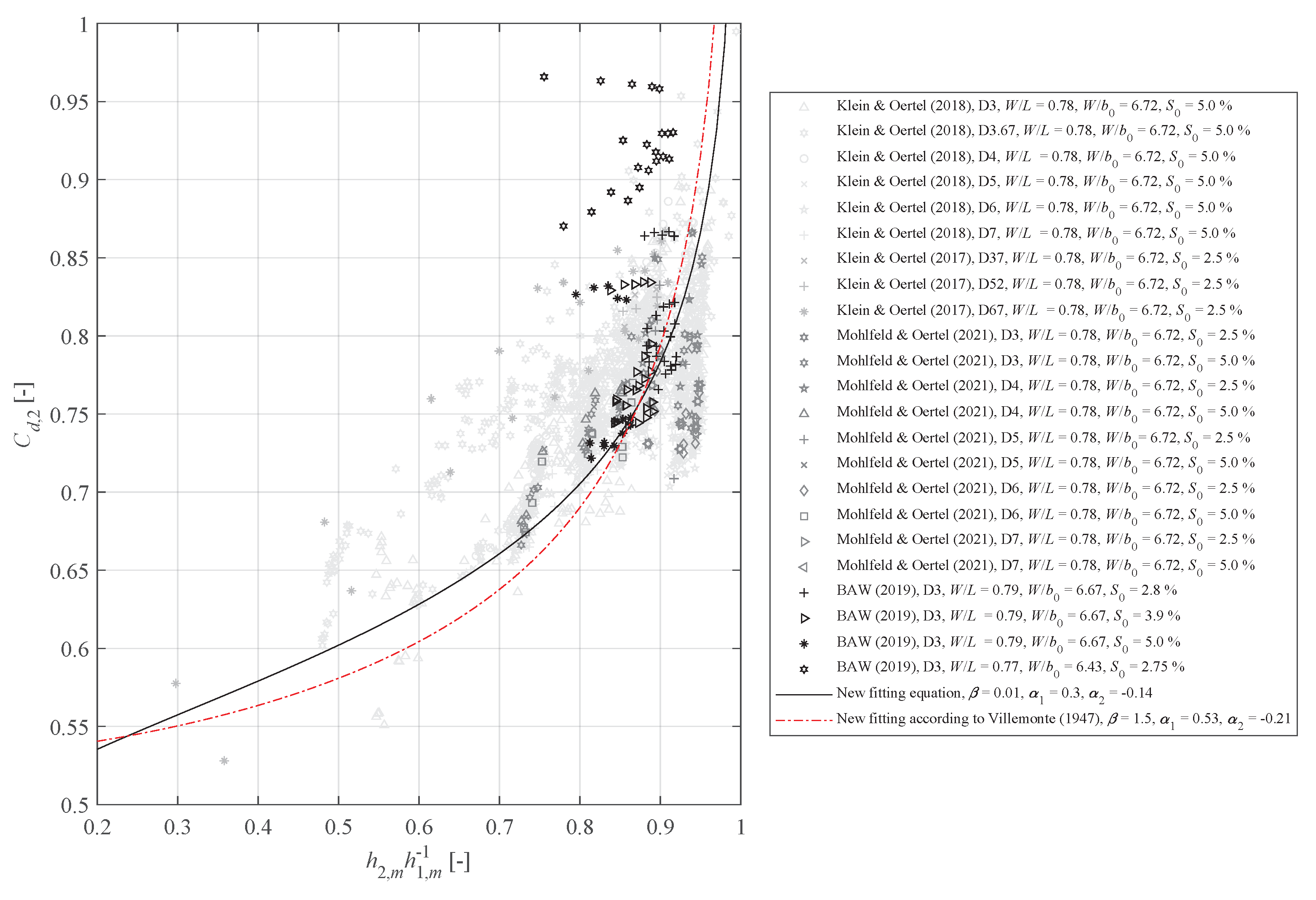
Figure 6 shows computed discharge coefficients $C_{d,2}$, determined via Equation (8) as a function of $h_{1,m}$, Q, and $v_{\max }$ for all data from the literature. Here, the maximum flow velocity $v_{\max }$ was calculated according to Torricelli (Equation (1)) with the mean water level difference $\Delta h_m=h_{1,m}-h_{2,m}$.

It can be observed from Figure 6 that the dispersion of calculated discharge coefficients for similar geometries becomes higher with increasing $h_{2,m}{h}_{1,m}^{-1}$. And current fitting parameters by [4,18] did not adequately reproduce discharge coefficients. Parameters by [4] show a better fit for $h_{2,m}{h}_{1,m}^{-1}$ > 0.8, but an overestimation could be noticed due to the small number of data points for small $h_{2,m}{h}_{1,m}^{-1}$ (see [3]). Ref. [18] produces acceptable results, but fitting parameters could be improved slightly. Furthermore, it can be noted that data of [25] show a wide dispersion of discharge coefficients, due to non-uniform flow conditions. Hence, it can be concluded that Equation (3) can determine discharge coefficients $C_{d,1}$ for Equation (2) with greater accuracy than discharge coefficients $C_{d,2}$ for Equation (8) [4].

Analogous to $C_{d,1}$, new fitting parameters for $C_{d,2}$ will be developed for the data sets of [3,6,23,25]. These fittings are used to calculate discharge coefficients according to Equation (3) for discharge calculations according to Equation (8). A fitting curve with $\beta$ = 1.5 was generated according to [18] (see Figure 7). Furthermore, a new fitting equation was generated:

$$C_{d,2,\mathrm{calc}}=0.3·{\left[1-{\left(\frac{h_2}{h_1}\right)}^{0.01}\right]}^{-0.14}$$

(10)

Fitting parameters ${\alpha }_1$ and ${\alpha }_2$ again were detemined using MATLAB’s curve fitting toolbox and plotted in Figure 7. It can be found that different fitting curves are in good agreement for $h_{2,m}{h}_{1,m}^{-1}$ > 0.80. Conseqently, $\beta$ = 1.5 can be used for $h_{2,m}{h}_{1,m}^{-1}$ > 0.80 in the geometrically defined range of validity. The new fitting according to [21] is very similar to the defined fitting equation for $C_{d,2}$ via [18]. There is less data in the range $h_{2,m}{h}_{1,m}^{-1}$ > 0.70 and more data collection is necessary for futher fitting statements.

For further investigations, the new fitting equation (Equation (10)) and data from Table 1 were used. Equation (10) was developed for better practical application and to guarantee a good fitting also for small values $h_{2,m}{h}_{1,m}^{-1}$ < 0.7. Parameters are extremely sensitive to small changes and hence, a careful fitting should be performed. In Equation (3), and Equation (10) respectively, ${\alpha }_1$ shifts the entire fitting curve up or down along the y-axis and does not change the slope of the curve. Contrarily, $\beta$ and ${\alpha }_2$ are used to change the curve’s radius or slope and to adopt the behavior in regions for smaller and larger $h_{2,m}{h}_{1,m}^{-1}$ values. Due to the existing data spreading the coefficient of determination $R^2$ might be no longer representative to describe the prediction accuracy; especially for $h_{2,m}{h}_{1,m}^{-1}$ > 0.7.

To further investigate developed fitting parameters, Figure 8 compares discharge coefficients for all data sets from the literature according to Equations (8) and (10). Additionally, Figure 8 presents percentage deviations for all data sets. It can be found that data by [7] shows the largest deviations with more than $-40$%, while discharge coefficients for [17] according to Equation (10) show a deviation of $-25$%. This can be explained again with geometrical differences for investigated model configurations. Nevertheless, it can be observed that some partial data of these publications are in a range of $\pm 20$%. Discharge coefficients of the remaining literature data can be generally found with a deviation of $\pm 20$%; only a few data of [23] are above $+20$%. It can be seen that the deviations for both Equations (9) and (10) are comparable within the data sets. Therefore, both approaches can be applied considering the geometric validity ranges and the defined $h_{2,m}{h}_{1,m}^{-1}$ ranges.

Overall, discharge coefficients can be calculated by using Equation (10) for slot pass basins with a basin geometry of 6.19 < $W{b}_0^{-1}$ < 6.72 and 0.77 < $W{L}^{-1}$ < 0.82 and guide elements listed in Table 1.

5. Summary and Conclusions

For an adequate VSP design, discharge coefficients are a major parameter to calculate resulting discharges on the structure. With the existence of two major discharge equations, namely Poleni and Torricelli, two various discharge coefficients $C_{d,1}$ and $C_{d,2}$ were analyzed separately. Both can be estimated using Villemonte’s empirical approach with fixed fittings. Numerous laboratory measurement campaigns investigating discharge coefficients were presented and analyzed to identify new fitting parameters. With these values conclusions about dependencies and accuracies were obtained.

Results show that discharge coefficients are highly dependent on the investigated basin geometry. A validity range of 6.19 < $W{b}_0^{-1}$ < 6.72 and 0.77 < $W{L}^{-1}$ < 0.82 could be defined for Equations (9) and (10). This definition was chosen due to similar percentage deviations of the fitting equation for a comparison of the Poleni and Torricelli discharge coefficients. Due to the similar deviations of the newly developed fitting equations with respect to the discharge coefficients, both approaches can be used for practical design. However, it should be noted that the new fitting equations can only be used under consideration of the validity ranges $W{L}^{-1}$, $W{b}_0^{-1}$ and $h_{2,m}{h}_{1,m}^{-1}$ as well as investigated guide elements.

In conclusion, fitting parameters for the Poleni or Torricelli approach are applicable in the defined range of validity. The datasets used from the literature are based on geometries which are frequently used in practical applications. Therefore, the new fitting equations, together with the validity ranges, can be used to design VSF. It could be confirmed that the parameter $\beta$ in the validity range with 1.5 according to [18,19,21] is applicable for $C_{d,1}$ with $h_{2,m}{h}_{1,m}^{-1}$ > 0.65 and for $C_{d,2}$ with $h_{2,m}{h}_{1,m}^{-1}$ > 0.80. For smaller $h_{2,m}{h}_{1,m}^{-1}$, further measurement data needs to be collected in order to be able to make a statement about the dependencies and influences of the geometric boundary conditions. It was also shown that ${\alpha }_1$ and ${\alpha }_2$ need to be estimated in order to develop an optimal fit for a given $\beta$. It was also shown that the discharge coefficients depend not only on the flow patterns/conditions or the geometry of the guide elements, but also on the basin and slot geometry. Despite the applicability, further investigation is required to extend the range of validity and to include more structural variations in the fitting equations.

References

- Water Framework Directive (WFD). Directive 2000/60/EC of the European Parliament and of the Council establishing a framework for the Community action in the field of water policy. Off. J. 2000. Available online: https://www.semanticscholar.org/paper/Directive-2000-60-EC-of-the-European-Parliament-and-Other/a3115d92366398ea8b94c69d847b952041ac886d (accessed on 12 January 2023).
- Deutsche Vereinigung für Wasserwirtschaft, Abwasser und Abfall e. V. (DWA). Fischaufstiegsanlagen und fischpassierbare Bauwerke—Gestaltung, Bemessung, Qualitätssicherung. DWA-Regelw. 2014. Available online: https://www.baufachinformation.de/merkblatt-dwa-m-509-mai-2014/mb/241832 (accessed on 12 January 2023). (In German).
- Mohlfeld, J.; Oertel, M. Ermittlung von Abflussbeiwerten zur hydraulischen Bemessung von Fischaufstiegsanlagen in Schlitzpassbauweise. WasserWirtschaft 2021, 2–3, 27–32. (In German) [Google Scholar] [CrossRef]
- Mohlfeld, J. Einfluss unterschiedlicher Leitelemente auf die Hydraulik in flach geneigten Schlitzpässen; Shaker Verlag: Herzogenrath, Germany, 2020. (In German) [Google Scholar]
- Wu, S.; Rajaratnam, N.; Katopodis, C. Structure of flow in vertical slot fishway. J. Hydraul. Eng. 1999, 125, 351–360. [Google Scholar] [CrossRef]
- Klein, J.; Oertel, M. Untersuchung von Einflussparametern auf die Abflussbemessung von Fischaufstiegsanlagen in Schlitzbauweise. Dresdner Wasserbauliche Mitteilungen 2017, 58, 291–300. (In German) [Google Scholar]
- Bermúdez, M.; Puertas, J.; Cea, L.; Pena, L.; Balairón, L. Influence of pool geometry on the biological efficiency of vertical slot fishways. Ecol. Eng. 2010, 36, 1355–1364. [Google Scholar] [CrossRef]
- Tarrade, L.; Texier, A.; David, L.; Larinier, M. Topologies and measurements of turbulent flow in vertical slot fishways. Hydrobiologia 2008, 609, 177–188. [Google Scholar] [CrossRef] [Green Version]
- Tarrade, L.; Pineau, G.; Calluaud, D.; Texier, A.; David, L.; Larinier, M. Detailed experimental study of hydrodynamic turbulent flows generated in vertical slot fishways. Environ. Fluid Mech. 2011, 11, 1–12. [Google Scholar] [CrossRef] [Green Version]
- Wang, R.W.; David, L.; Larinier, M. Contribution of experimental fluid mechanics to the design of vertical slot fish passes. Knowl. Manag. Aquat. Ecosyst. 2010, 396, 2. [Google Scholar] [CrossRef]
- Stamou, A.I.; Mitsopoulos, G.; Rutschmann, P.; Biui, M.D. Verification of a 3D CFD model for vertical slot fish-passes. Environ. Fluid Mech. 2018, 18, 1435–1461. [Google Scholar] [CrossRef]
- Tuhtan, J.A.; Fuentes-Pérez, J.; Toming, G.; Schneider, M.; Schwarzenberger, R.; Schletterer, M.; Kruusmaa, M. Man-made flows from a fish’s perspective: Autonomous classification of turbulent fishway flows with field data collected using an artificial lateral line. Bioinspiration Biomim. 2018, 13, 046006. [Google Scholar] [CrossRef] [PubMed]
- Pope, S.B. Turbulent Flows; Cambridge University Press: Cambridge, UK; New York, NY, USA, 2000. [Google Scholar]
- Liu, M.; Rajaratnam, N.; Zhu, D.Z. Mean Flow and Turbulence Structure in Vertical Slot Fishways. J. Hydraul. Eng. 2006, 132, 765–777. [Google Scholar] [CrossRef]
- Rajaratnam, N.; van der Vinne, G.; Katopodis, C. Hydraulics of Vertical Slot Fishways. J. Hydraul. Eng. 1986, 112, 909–927. [Google Scholar] [CrossRef]
- Puertas, J.; Pena, L.; Teijeiro, T. Experimental Approach to the Hydraulics of Vertical Slot Fishways. J. Hydraul. Eng. 2004, 13, 10–23. [Google Scholar] [CrossRef]
- Rajaratnam, N.; Katopodis, C.; Solanki, S. New design for vertical slot fishways. Can. J. Civ. Eng. 1992, 19, 402–414. [Google Scholar] [CrossRef]
- Fuentes-Pérez, J.; Sanz-Ronda, F.; Martínez de Azagra Paredes, A.; García-Vega, A. Modeling Water-Depth Distribution in Vertical-Slot Fishways under Uniform and Nonuniform Scenarios. J. Hydraul. Eng. 2014, 140, 06014016. [Google Scholar] [CrossRef] [Green Version]
- Fuentes-Pérez, J.; García-Vega, A.; Sanz-Ronda, F.; Martínez de Azagra Paredes, A. Villemonte’s approach: A general method for modeling uniform and non-uniform performance in stepped fishways. Knowl. Manag. Aquat. Ecosyst. 2017, 418, 23. [Google Scholar] [CrossRef] [Green Version]
- Krüger, F.; Heimerl, S.; Seidel, F.; Lehmann, B. Ein Diskussionsbeitrag zur hydraulischen Berechnung von Schlitzpässen. WasserWirtschaft 2010, 3, 30–36. (In German) [Google Scholar] [CrossRef]
- Villemonte, J.R. Submerged-Weir Discharge Studies. Eng. News Rec. 1947, 139, 866–869. [Google Scholar]
- Clay, C.H. Design of Fishways and Other Fish Facilities, 2nd ed.; Clay, C.H., Ed.; Department of Fisheries of Canada: Ottawa, ON, Canada, 1961.
- Federal Waterways Engineering and Research Institute (Bundesanstalt für Wasserbau—BAW). Dataset of Investigated Slot Passes. 2019. Available online: henry.baw.de (accessed on 12 January 2023).
- Höger, V.; Prinz, F.; Meltzer, J.V. Die Variabilität der Fließgeschwindigkeit in Schlitzpässen. HENRY-Hydraul. Eng. Respository 2020, 106, 23–32. (In German) [Google Scholar]
- Klein, J.; Oertel, M. Influence of Inflow and Outflow Boundary Conditions on Flow Situation in Vertical Slot Fishways. IAHR Int. Symp. Hydraul. Struct. 2018, 7. Available online: https://digitalcommons.usu.edu/cgi/viewcontent.cgi?article=1166&context=ishs (accessed on 12 January 2023).
Figure 1.
Photograph of an examplary vertical slot pass at a weir in North-Rhine Westphalia, Germany.
Figure 2.
Flow patterns in a VSF based on [5], (left:) flow pattern 1, (right:) flow pattern 2.
Figure 4.
Discharge coefficients and new fitting equations according to Equation (3) based on Poleni (Equation (2)) [2,3,6,23,25].
Figure 5.
Comparison of calculated discharge coefficients according to Equations (2) and (9) with error bounds of ±10% and ±20% [3,6,7,16,17,20,23,25].
Figure 6.
Discharge coefficients and existing fitting equations according to Equation (3) based on Torricelli (Equation (8)) [3,4,6,7,16,17,18,20,23,25].
Figure 7.
Discharge coefficients and new fitting equations according to Equation (3) based on Torricelli (Equation (8)) [3,6,23,25].
Figure 8.
Comparison of calculated discharge coefficients according to Equations (8) and (10) with error bounds of ±10% and ±20% [3,6,7,16,17,20,23,25].