Investigations of Multi-Platform Data for Developing an Integrated Flood Information System in the Kalu River Basin, Sri Lanka

Abstract

Flood early warning systems (FEWS) are crucial for flood risk management; however, several catchments in the developing world are still far behind in all aspects of FEWS and thus, they encounter devastating damage recurrently due to limitations in data, knowledge, and technologies. This paper presents a catchment-scale integrated flood information system by incorporating present-day multi-platform data and technologies (e.g., ground and satellite rainfall observation, ensemble rainfall forecasts, and flood simulation) and evaluates their performance in a poorly gauged prototype basin (i.e., the Kalu River basin). Satellite rainfall products obtained in real time (GSMaP-NOW) and near-real time (GSMaP-NRT) can detect heavy rainfall events well and bias-corrected products can further improve rainfall estimations and flood simulations. Particularly, GSMaP-NRT, which outperformed GSMaP-NOW in both rainfall and discharge estimations, is suitable for near-real-time flood-related applications. Ensemble rainfall forecasts showed good performance in predicting alarming signals of heavy rainfall and peak flow with uncertainties in the amounts and timings of the events. Information derived from both satellite and ensemble forecasts on heavy rainfall, simulated flood signals, and their possible range of probabilities is promising and can help minimize the data gaps and improve the knowledge and technology of experts and policy-makers in poorly gauged basins.

1. Introduction

Climate change continues to increase the frequency and severity of flood and storm disasters, which are found to be a major impediment to sustainable development [1,2,3]. Flood Early Warning Systems (FEWS) are identified as one of the effective methods for flood risk management and they are crucial for the achievement of the Sendai Framework for Disaster Risk Reduction targets and the Sustainable Development Goals advocated by the United Nations International Strategy for Disaster Reduction [4]. Nevertheless, a recent report has indicated that low- and middle-income countries, which suffer severe flood damage, are still far behind in the necessary aspects of FEWS (i.e., data collection, forecasting tools, and communication methods), whereas developing countries appear to be relatively progressing [5]. FEWS services are proven life-savers; however, they are woefully insufficient for those who need them most, particularly in Africa and the South- and Southeast-Asian regions due to data unavailability and the technology–knowledge gaps, which have resulted in enormous fatal and economic losses in recent flood events (e.g., 2022: Pakistan, 2021: Southeast Asia, 2020: Jakarta, 2018: East Africa, 2018: Kerala, 2016: India, and 2016/2017: Sri Lanka). Hence, the UN and the World Meteorological Organization (WMO) unveiled an urgent action plan at the 2022 UN Climate Change Conference (COP27) to ensure the availability of FEWS for all communities to shift from reactive measures to a proactive flood management approach within five years [6].

In fact, several initiatives have developed FEWS at the global scale using present-day science and technologies, e.g., the GEOGloWS ECMWF streamflow forecasting [7], the Global Flood Forecasting and Information System (GLOFFIS) [8], and the Global Flood Awareness System (GloFAS) [9] to support preparatory measures for flood events worldwide, particularly in large trans-national river basins. Though global FEWS are useful for the least-developed and developing countries, they lack in providing accurate flood-related information (e.g., flood onset, peak flow, and inundation) at the medium or small catchment scales due to uncertainties in coarse resolution rainfall forecasts and challenges in integrating locally available knowledge and information at the global scale and calibrations and verifications of flood model outputs [10]. Moreover, several studies have investigated and developed advanced concepts of FEWS at the national or catchment scales, mostly in developed countries (e.g., the U.S.A. [11], Europe [12,13], Australia [14], and Japan [15,16]), which maintain the high-quality and quantity of in-situ and radar observation networks as well as advanced rainfall forecasting techniques; however, the applicability, affordability, and verifications of such systems in poorly gauged regions have not been addressed.

Preferably, a catchment-scale Integrated Flood hazard Information System (IFIS) should have the following essential components capable of (a) adequate real-time rainfall observation, (b) quantitative rainfall prediction, (c) runoff and inundation simulation, and (d) data analysis and dissemination. Various reports have also been published on the design, implementation, and operation of FEWS in developing regions (e.g., Africa and South-east Asia); however, only a few scientific studies have reported on the verifications of rainfall and flood forecasts at catchment scales due to data unavailability, coarser resolution model outputs, and the technology–knowledge gap [17,18,19,20,21,22]. As a result, many river basins in those regions are still behind in implementing FEWS and proactive flood management approaches. To move forward and support the UN agenda on FEWS for all within the next five years (2023–2017) promptly, there is a great need for the development and verification of catchment-scale IFIS by taking advantage of the latest updates on ground and satellite observation technologies and rainfall forecasting methods to fill the data and knowledge–technology gaps and support reliable timely decision-making processes in developing regions. Hence, this research presents a basin-scale IFIS and investigated its performance by utilizing present-day ground and satellite observation techniques and numerical models to gain confidence in the system. This is the first study to investigate multi-platform extreme flood events data (i.e., ground, satellite, bias-corrected outputs, and numerical model outputs) simultaneously in a single study and integrate them to implement an IFIS in developing regions. The following paragraphs briefly review the present-day status of each component of IFIS (except the data analysis and dissemination component) and their applications in developing regions.

Real-time or near-real-time rainfall data with high spatial and temporal resolutions are a prerequisite for flood monitoring, though rarely available in most river basins. Nevertheless, freely-available global satellite precipitation products (SPPs) have the potentials to be used for real-time rainfall monitoring and flood warning in poorly gauged basins, and thus are widely promoted by global and regional agencies [23,24,25,26]; however, they contain spatially and temporarily varying biases due to indirect measurements and interpolation methods to fill microwave observation gaps, they cannot be applied for reliable flood parameter estimation without bias corrections, and thus, the information from ground gauges need to be incorporated to improve the quality of SPPs in flood applications [27,28,29,30]. Particularly, real-time hourly or daily gauge data can help improve the spatially and temporarily varying biases of SPPs for real-time applications and thus, additional investments are required for infrastructure development and maintenance. Zhou et al. (2022) [31] proposed a gauge network design method for finding a threshold and its configurations necessary for effective bias correction of SPPs. As an alternative approach, this research used a satellite rainfall climatology map that provides reliable rainfall distributions over the basin to find a minimum gauge threshold and locations for encouraging smart investments in data-poor regions. In addition, the Japan Aerospace Exploration Agency (JAXA) has recently provided the first-ever real-time SPPs with the shortest latency time (~0 h) [26]. However, its performance for flood applications is yet to be investigated. Thus, this research investigated the performance of JAXAs real-time SPPs.

Quantitative rainfall forecasts, which are necessary for early warning and preparedness, show a steady improvement in the forecast skills of extreme weather conditions [32,33,34,35]. Most of the rainfall forecast systems in developing countries are based on the deterministic method, which does not offer information across more extensive forecasting ranges with uncertainty estimations [36]. Ensemble forecasts can provide a better skill score than deterministic forecasts and, therefore, can provide added values for flood forecasting, early warning, and emergency operations [37,38,39,40,41]. Ensemble forecasting skills are progressing faster and developing countries are able to assess the ensemble data streams freely; however, only a few countries in the developing world have progressed in the ensemble rainfall prediction system, whereas their usage for streamflow forecast is not widely addressed in many regions [22]. Recent studies using various ensemble forecasts in different river basins showed that a streamflow forecast could provide reliable skills at a 1–5-day lead [42] and that the peak discharge correlated well with observed data [43], whereas the skill of forecasts in capturing extreme precipitation events was poor [44]. Therefore, more studies are necessary to verify ensemble rainfall forecasts and quantify the uncertainties to gain confidence and incorporate it in catchment scale FEWS in many developing regions.

Furthermore, physically based distributed hydrological models with the capability of simulating rainfall–runoff–inundation processes are very effective tools for obtaining crucial flood-related information (i.e., peak flow, inundation depths, and extents) compared to conceptual or kinematic wave hydrological models [45,46,47]. However, in many practical cases, the applications of these models only consider water-budget-related processes for simplifications and, thus, overlook dominant hydrological processes such as evapotranspiration and soil moisture dynamics, which consequently leads to more uncertainties in simulated flood-related parameters such as the timing of the flood onset, peak flows, and inundation depths [48]. As a result, this study employed the water and energy budget-based rainfall–runoff–inundation (WEB-RRI) model, which has several merits, including physical formulations for evapotranspiration fluxes and soil moisture dynamics to improve the accuracy of soil water storages and reduce model-related uncertainties and the compatibility with numerical weather models to estimate basin responses to model forcing data directly [48].

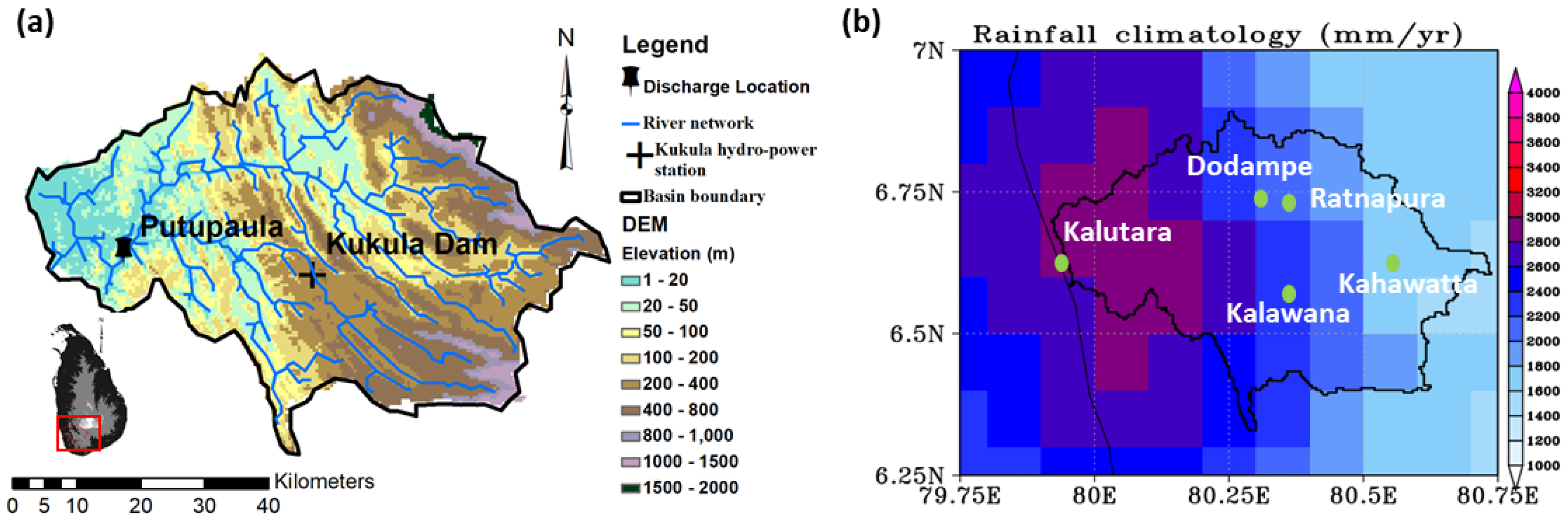
2. The Kalu River basin of Sri Lanka

This study selected the Kalu River basin as a pilot river basin. The basin is located in the southwestern part of Sri Lanka (Figure 1a), has a catchment area of ~2800 km², and receives an annual average rainfall of 4000 mm. It experiences frequent flood damage due to heavy rainfall, topographic characteristics, and demographic situations. In recent years, (e.g., 2012, 2014, 2017, 2018, and 2021), the basin has witnessed several flooding events; the 2017 flood was particularly devastating. The basin has no large flood-storage facilities or dams. There have been several feasibility studies and proposals (e.g., the Kukule reservoir, the Malwale reservoir, and dry dams on tributaries) for mitigating recurrent flood damage in this basin; however, none of them were executed due to economic and political conditions. A previous study on this basin indicated the necessity to either control floods or increase the people’s resilience to live with floods and proposed probability relationships for forecasting downstream water levels using upstream water level data [49]. Presently, flood warnings are issued based on rainfall forecasting and/or in-situ river water-level records.

3. Flood Information System, Data, and Model Set-Up

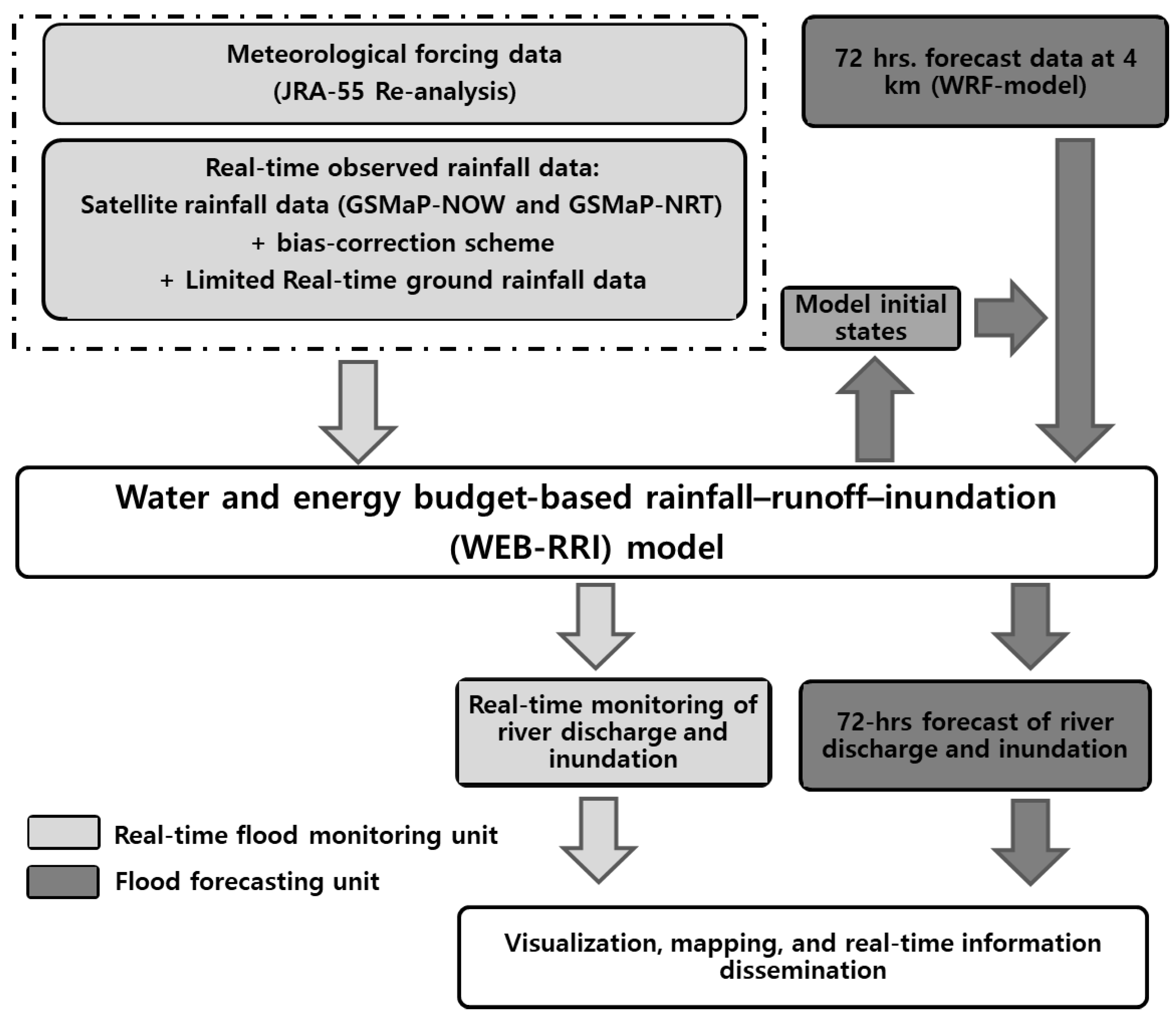
3.1. System Components and Data Integration

A schematic diagram of the proposed system that integrates multi-platform data and their interactions with the system components is shown in Figure 2. The system has two major components: a real-time flood-monitoring unit and a flood-forecasting unit. The first one merges limited real-time ground rainfall observation with real-time satellite data to generate real-time bias-corrected rainfall data and then prepares the Japanese 55-year Reanalysis (JRA-55) data for other forcing data. The second component utilizes 72 h of quantitative ensemble rainfall forecasts as well as other forcing data from the Numerical Weather Prediction (NWP) model. The WEB-RRI model was used as a flood simulator. The real-time flood monitoring unit was executed every hour, whereas the flood forecasting unit was executed every 24 h. The model’s initial states (i.e., river flow, slope flow, soil, and vegetation water storage) for forecast simulations were obtained from the flood monitoring unit driven by bias-corrected SPPs.

3.2. Meteorological Data

3.2.1. Japanese Reanalysis (JRA) Data

Meteorological forcing inputs for the WEB-RRI model, such as air temperature, specific humidity, wind speed, downward shortwave radiation, longwave radiation, and surface pressure, were obtained from the Japanese 55-year Reanalysis (JRA-55) data at a 3 h temporal resolution and 0.125° spatial resolution [50]. These meteorological forcing data were resampled to model grid resolutions of ~450 m and a model temporal resolution of 1 h using a linear interpolation method.

3.2.2. In-Situ Rainfall

For this study, we installed a real-time hourly rainfall observing and transmitting system in the Kalu River basin with financial support from JAXA to maximize the applicability of GSMaP products. As stated in the Introduction, the density and locations of rain gauges are the most crucial in deploying a real-time gauge network, and the estimation of a minimum threshold number of gauges for the bias-correction of SPPs mainly depends on the rainfall distribution pattern and basin size. A rainfall climatology map was developed from 15 years of (2001–2015) GSMaP-NRT data and plotted in Figure 1b. The figure illustrates the rainfall heterogeneity in the basin, i.e., the middle and downstream regions received higher rainfall amounts, whereas the upstream regions received relatively lesser rainfall. Therefore, a total of five real-time gauges (one in upstream, one in downstream, and three in the middle region) were installed in this basin (density ~560 km²/gauge), considering the rainfall pattern, river tributaries, and secure premises. The locations of the real-time rainfall observing and transmitting systems are shown in Figure 1b and listed in

Table 1. Coordinates of the rainfall and discharge gauge locations.

No.	Station Name	Latitude (N)	Longitude (E)
1	Kahawatta	6.6	80.58
2	Kalawana	6.54	80.38
3	Ratnapura	6.72	80.38
4	Dodampe	6.73	80.32
5	Kalutara	6.6	79.95
6	Putupaula (discharge only)	6.6	79.95

.

3.2.3. Satellite Rainfall Products and Bias Correction

In this research, we used real-time and near-real-time GSMaP products, which are available at 0.1° spatial and 1-h temporal resolutions. GSMaP data integrate geostationary infrared data with limited low-earth-orbiting passive microwave satellite data to fill spatial and temporal gaps [51]. GSMaP uses an infrared–microwave combined algorithm [52], a backward-and-forward morphing technique from infrared images [53], and a Kalman filter [54] for estimating precipitation. GSMaP-NRT is available with about 4 h latency, and GSMaP-NOW is available with the shortest latency (~0 h) and is very useful for flood-related applications.

Software (i.e., GSMaP-IF2) developed by the NTT-DATA corporation of Japan and JAXA was used in this study to improve spatial and temporal biases. As shown in Figure 3, GSMaP-IF2 uses an algorithm that takes ground-observed rainfall data (hourly or daily) and GSMaP data (hourly) as primary inputs. The algorithm has three steps in estimating merged rainfall products: (a) geo-location correction, (b) weight calculation, and (c) rainfall intensity correction.

Geo-location correction: The combined passive microwave and IR-based SPPs (i.e., GSMaP and IMERG), which use morphing techniques, experience spatial shifting of a rainfall system [28,55]. To eliminate erroneous shifting, ground gauges are combined into one or several groups, depending on the number of gauges and their locations, and then the correlation coefficient between ground rainfall and the corresponding GSMaP rainfall is calculated for each group separately. When estimating the correlation coefficient for an individual group, the possibility of shifting within a given range (~3–5 grids or 30–50 km in all eight directions) is considered. Consequently, the best correlation coefficient is identified by comparing all the calculation results, and the corresponding shift is applied to the GSMaP data.

Weight calculation: An active area from each observatory (e.g., a radius of ~100–200 km) is defined for estimating weights. The product of the inverse distance and the elevation difference is set as the weight for each grid.

Rainfall intensity correction: Two types of factors (i.e., scale and offset) are calculated as microwave rainfall estimations, which are weak for light rains. If the GSMaP rainfall intensity is less than 10 mm/day, the offset factor (i.e., difference) is considered; otherwise, the scale factor (i.e., ratio) is considered. Finally, the corrected rainfall is calculated as follows:

$$\begin{array}{c}Corrected GSMaP data\\ =\left\{\begin{array}{c}GSMaP raw data * scale factor * weight; if rainfall > 10 \mathrm{mm}/\mathrm{day})\\ (GSMaP raw data + Offset) * weight; if rainfall < 10 \mathrm{mm}/\mathrm{day})\end{array}\right.\end{array}$$

(1)

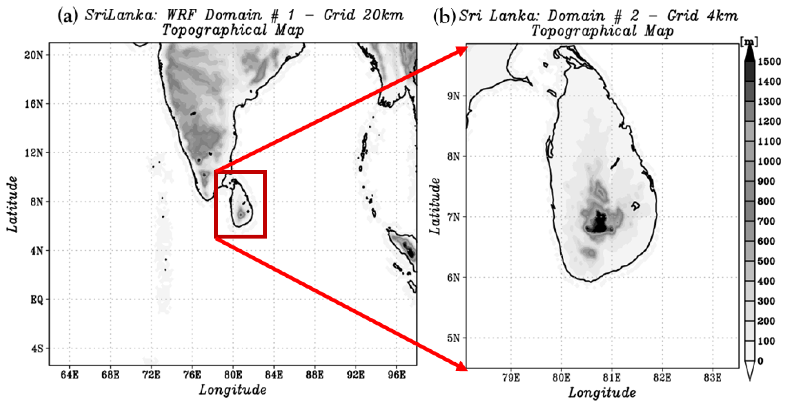
3.2.4. Meteorological Rainfall Forecasts

The Weather Research and Forecasting (WRF) model [56] was employed for downscaling global-scale forecasts to basin-scale. Regional simulations were conducted with a 20 km horizontal resolution and then downscaled to a 4 km horizontal resolution (Figure 4). The outer domain (4000 km × 3000 km) was calibrated with newer Tiedtke cumulus and Lin cloud microphysics schemes, whereas the inner domain (600 km × 600 km) was calibrated with Lin cloud microphysics schemes. The initial and boundary conditions were obtained from the Global Ensemble Forecast System (GEFS version 10) of the National Centers for Environmental Prediction (NCEP), which produces 80 perturbation forecasts per day, 20 per cycle (00UTC, 06UTC, 12UTC, and 18UTC), at T254L42 (~52 km) resolution for eight days [57]. The control and ensemble members in even numbers (10 out of 20 ensemble members) were selected based on a cluster analysis to reduce the computational time [58], and the downscaling experiments were set up to produce ensemble forecasts for the next 72 h.

3.3. Hydrological Data and Model

3.3.1. Hydrological Data

Topographic Data, Soil Type, Land Use, and Vegetation Data

This study used 15 arc-seconds (~450 m) of hydrologically conditioned data (i.e., topographic data, flow directions, and flow accumulation) obtained from the U.S. Geological Survey’s hydrological data and maps based on the Shuttle Elevation Derivatives at multiple Scale (HydroSHEDS) [59]. Soil-type and soil-related parameters (e.g., saturated hydraulic conductivity for surface soil, root zone, groundwater zone, saturated soil moisture content, residual soil moisture content, and Van Genutchen parameters, i.e., alpha and n) were obtained from the Food and Agriculture Organization (FAO) at a 9 km spatial resolution (http://www.fao.org (accessed on 14 January 2006)). The land-use data for Simple Biosphere Model (SiB2) was obtained from the U.S. Geological Survey’s global datasets with a spatial resolution of 1 km. The 08-day composites Terra satellite’s Moderate Resolution Imaging Spectroradiometer (MODIS) global products (MOD15A2) of Leaf Area Index (LAI) and Fraction of Photo-synthetically Active Radiation (FPAR) at a 1 km horizontal resolution were obtained from NASAs data archives (https://search.earthdata.nasa.gov/ (accessed on 11 March 2015)).

Discharge and Inundation Data

This research used the discharge data collected at the Putupaula station (Figure 1a and Table 1) by the Irrigation Department. The water levels prescribed by the Irrigation Department of Sri Lanka for alert, minor flood, and major flood situations at the Putupula gauging station are 3 m (~700 m³/s), 4 m (~1000 m³/s), and 5 m (~1400 m³/s) from the local datum, respectively. Inundation data were derived from the VH-polarization of space-borne Sentinel-1 Synthetic Aperture Radar (SAR) observation. The advantage of using VH-polarization over VV polarization for water body classification is that it is less affected by water surface waves and terrain slopes. In this study, SAR data of 10 m resolution were obtained and resampled to model grids (i.e., 500 m). A pixel was classified as a floodwater pixel when its value at VH polarization decreases by 5 dB or lower after a flood event.

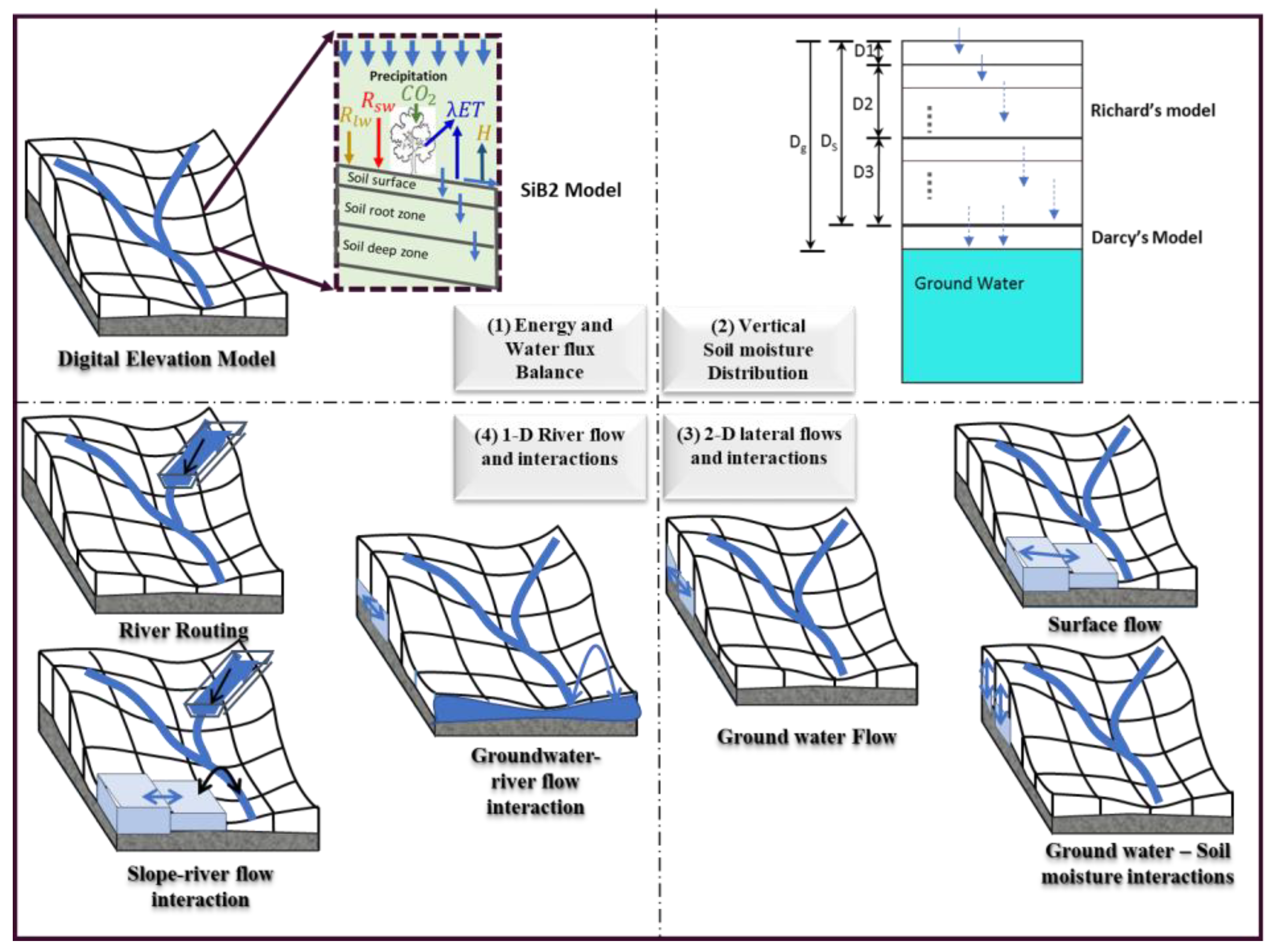
3.3.2. Hydrological Model and Model Setup

The structure of the WEB-RRI model (Figure 5) developed by Rasmy et al. (2019) [48] was divided into four major modules: (i) the model grid-based SiB2 module for the vertical energy and water flux transfer between land and atmosphere [60,61]; (ii) the vertical soil moisture distribution and groundwater recharge module [62]; (iii) the 2-D diffusive wave flow module for surface and groundwater flow module; and (iv) the 1-D diffusive wave river flow module [47]. The interactions between surface flow and river flow, groundwater flow and soil moisture contents, and groundwater flow and river flow were also incorporated into the model. The shape of the river channel was assumed to be rectangular. The model grid resolution was ~450 m, and the temporal resolution was 1 h. The WEB-RRI model setup, calibration, and validation for the Kalu River basin were conducted in the previous study [48], which evaluated the model’s performance comprehensively using long-term rainfall data, river discharge data, satellite-derived ET data, and inundation extents observations. Therefore, the same model was implemented for real-time flood monitoring and forecasting applications. The model formulation and verifications are referred to in Rasmy et al. (2019) [48].

3.4. Evaluation Indices

This study used following datasets for the verifications of the system outputs; rainfall data obtained from the real-time automated rain gauge network are used for the verification of the GSMaP data; bias-corrected GSMaP gridded data are used for the verification of ensemble forecast data; recorded river gauge data are used for verification of the simulated river flow; and SAR data are used for the verification of the simulated inundation extents.

3.4.1. Rainfall and Discharge Evaluation Indices

Mean Bias Error (MBE), Root Mean Square Error (RMSE), Nash–Sutcliffe Efficiency Coefficient (Nash), the ensemble spread (i.e., the unbiased estimator of the standard deviation), and the Brier Score (BS) were used for evaluating model estimations. The ensemble spread, a measure of the difference between the members and the ensemble mean, is represented by the standard deviation. The Brier Score [63], a measure of the accuracy of probabilistic forecasts, is typically used when the outcome of a forecast is binary—whether the outcome occurs or not.

MBE is defined as the following:

$$MBE=\frac{\sum (S_i-O_i)}{N}$$

(2)

RMSE is defined as the following:

$$RMSE=\sqrt{\frac{\sum {{(O}_i-S_i)}^2}{N}}$$

(3)

Nash is defined as the following:

$$Nash=\frac{\sum {(O_i-\stackrel{-}{O})}^2-\sum {{(O}_i-S_i)}^2}{\sum {(O_i-\stackrel{-}{O})}^2}$$

(4)

Spread is defined as the following:

$$Spread=\sqrt{\frac{\sum {(S_m-\stackrel{-}{S})}^2}{(M-1)}}$$

(5)

Brier Score (BS) is defined as the following:

$$BS=\frac{\sum {\left[\mathrm{P}\right(S_m)-\mathrm{P}\left(O_i\right)]}^2}{M}$$

(6)

where $O_i$ is the observation at the ith time, $\stackrel{-}{O}$ is the averaged observation over the time, $S_i$ is the simulated value at the ith time, $S_m$ is the simulated value for the mth member, $\stackrel{-}{S}$ is the ensemble mean, P$\left(S_m\right)$ is the forecast probability from 0 to 1, P$\left(O_i\right)$ is the event outcome (0 or 1), N is the number of data, and M is the number of ensembles.

3.4.2. Flood Extent Evaluation Indices

The spatial correlation between the model-simulated and observed flood inundation extents was evaluated using the fit index (FI) and the correctness index (CI). The FI (%) and CI (%) are defined as follows [64,65]:

$$FI=\frac{A_{omfit}}{A_o+A_m-A_{omfit}}\times 100$$

(7)

$$CI=\frac{A_{omfit}}{A_o}\times 100$$

(8)

where $A_o$ is the observed flood inundation area, $A_m$ is the model-simulated flood inundation area, and $A_{omfit}$ is the overlapped flood inundation area (fit area) between the observed and simulated inundation extents.

4. Results

The Kalu River basin experienced a historic (major) flood in May 2017 due to an unprecedented heavy rainfall event, which caused devastating damage. The basin also experienced a minor flood in May 2018. Hence, the performance of the IFIS was evaluated for the selected three cases (i.e., major flood, minor flood, and false alarm), as listed in

Table 2. The selected flood events for the system performance evaluation.

No.	Flood Event	Event Period
1	Historical (major) flood	25 May 2017~2 June 2017
2	Minor flood	20 May 2018~28 May 2028
3	False alarm	24 May 2018

.

4.1. Rainfall Observation and Forecasts

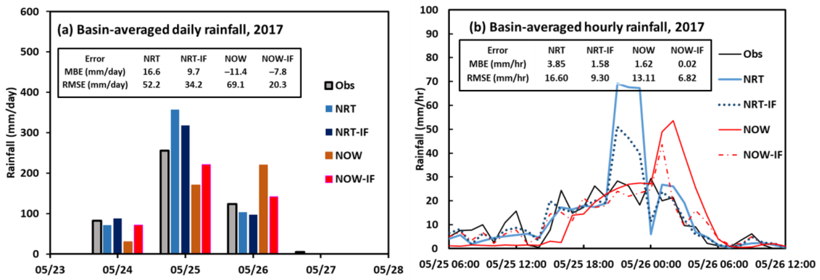
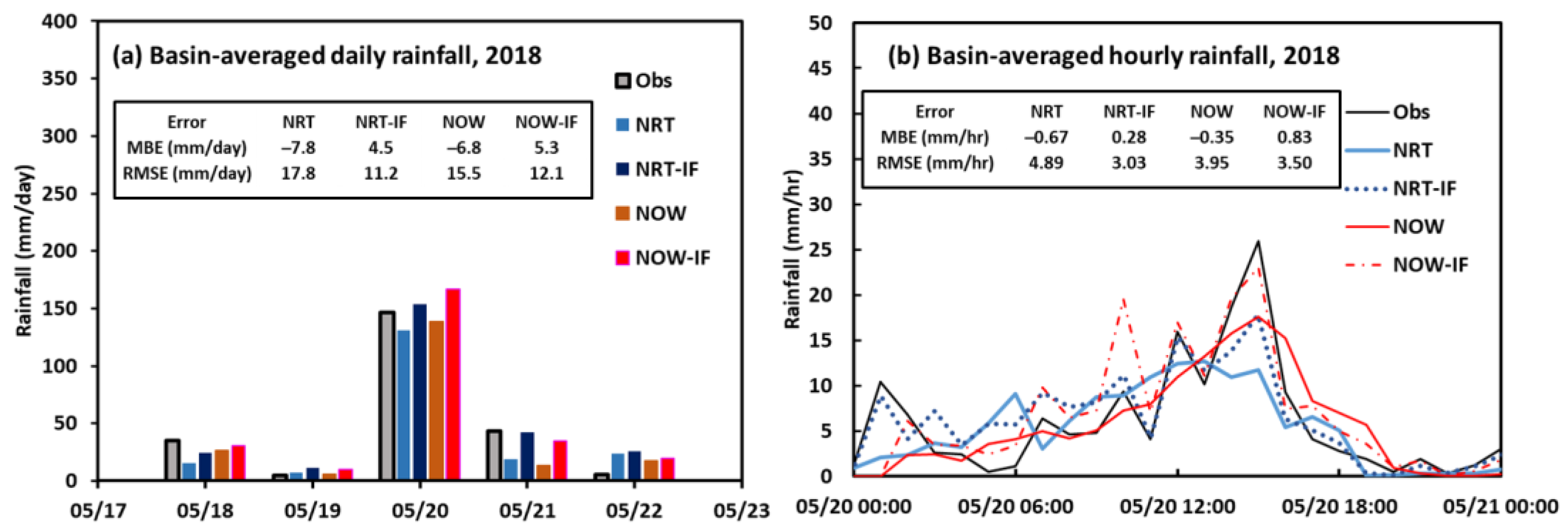
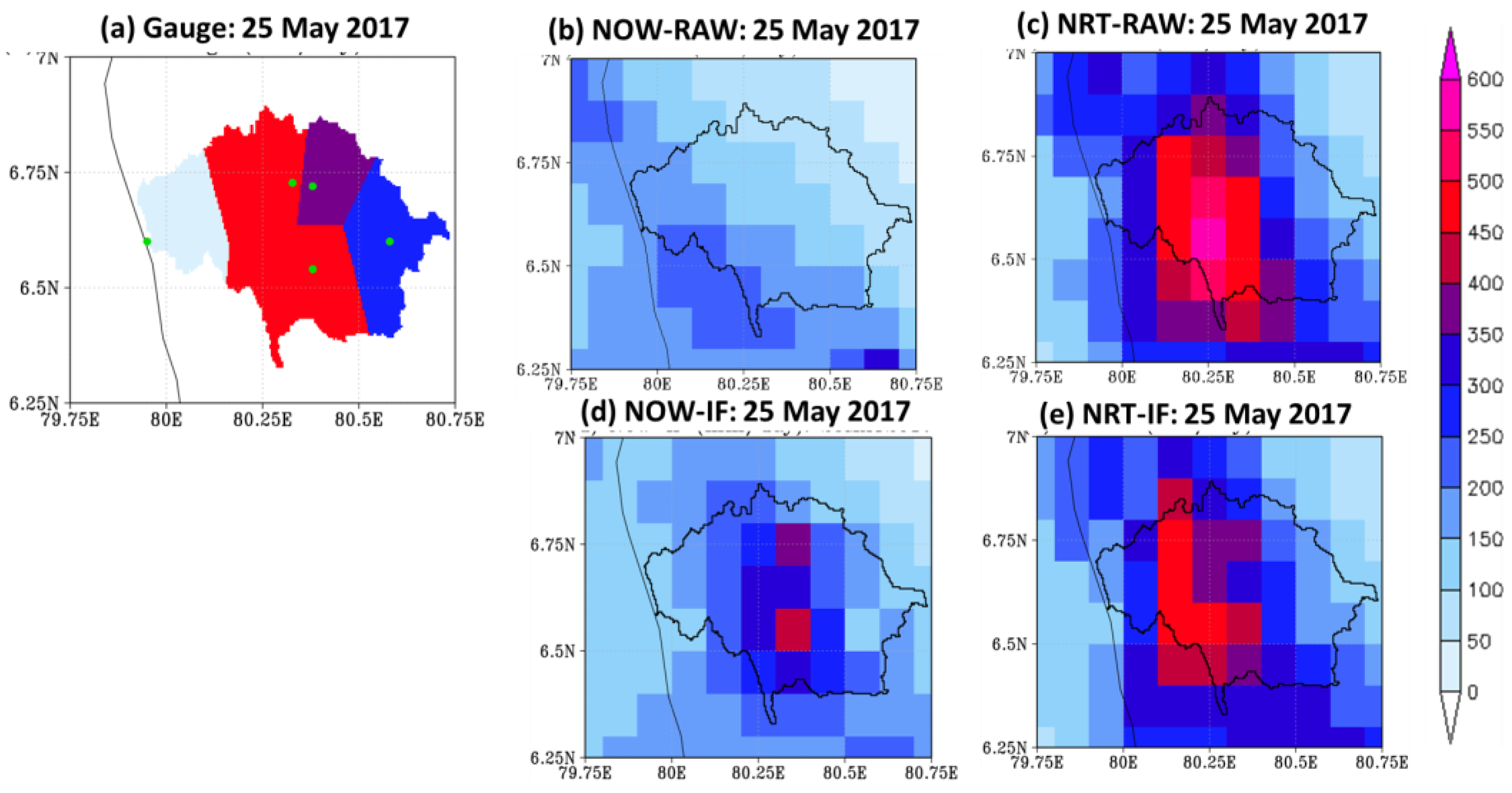
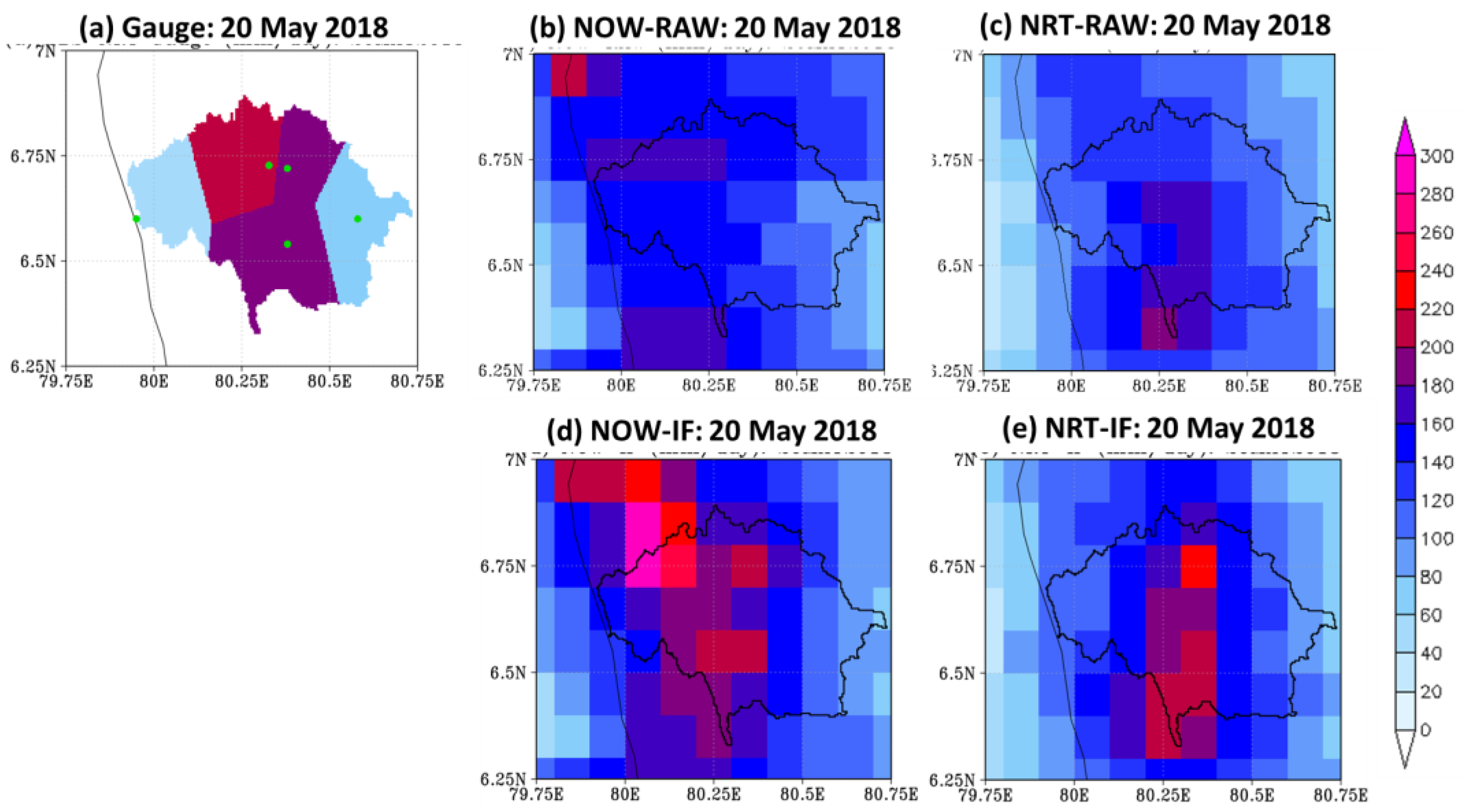
4.1.1. Satellite Rainfall (GSMaP) Products

Figure 6a compares basin-averaged GSMaP daily rainfall products with in-situ data for the May 2017 event. The error statistics for both raw and bias-corrected rainfall products were also shown in the corresponding figures. As shown in the figure, the basin-averaged GSMaP-NRT rainfall was overestimated by ~100 mm/day (~40%), whereas the GSMaP-NOW rainfall was underestimated by ~100 mm/day (~35%) compared to the in- situ rainfall on 25 May (i.e., the heaviest rainfall day). On the previous day, 24 May, the rainfall from GSMaP-NRT was comparable to the in-situ rainfall, whereas the rainfall from GSMaP-NOW was underestimated. On the next day, 26 May, GSMaP-NRT still showed a good match with the in-situ data, whereas GSMaP-NOW overestimated the basin-averaged rainfall. The estimated error statistics for the 3-day event period were relatively higher for GSMAP-NOW (i.e., MBE = −11.4 mm/day and RMSE = 69 mm/day) compared to GSMaP-NRT (i.e., MBE = 16.6 mm/day and RMSE = 52 mm/day). Similarly, both the rainfall amounts from GSMaP-NRT and GSMaP-NOW for the heaviest rainfall day of the May 2018 event (i.e., 20 May) were reasonably better, with slight underestimations (5~10%) (Figure 7a). The estimated error statistics were slightly better for GSMAP-NOW (i.e., MBE = −6.8 mm/day and RMSE = 17 mm/day) compared to GSMaP-NRT (i.e., MBE = −7.8 mm/day and RMSE = 15 mm/day). As also shown in Figure 6a and Figure 7a, the error statistics for bias-corrected GSMaP-NRT (hereafter NRT-IF) and bias-corrected GSMaP-NOW (hereafter NOW-IF) products at the basin scale improved significantly compared to their raw products for both events.

Information on the hourly rainfall intensities is crucial for flood-related applications. Figure 6b compares the hourly rainfall intensities between basin-averaged GSMaP products and the in-situ data for the May 2017 event. The overestimation from GSMaP-NRT was clearly seen for a short period (21 UTC to 23 UTC on 25 May). On the other hand, GSMaP-NOW underestimated the rainfall intensities from 06 UTC to 12 UTC on 25 May and overestimated them from 00 UTC to 06 UTC on 26 May. The bias-corrected products showed improvements on both MBE and RMSE for both products (i.e., MBE = 1.58 mm/h, RMSE = 9.3 mm/h for NRT-IF; MBE = 0.02 mm/h, RMSE = 6.82 mm/h for NOW-IF). As shown in Figure 7b, though the peak rainfall intensities were underestimated by both GSMaP products during 12UTC–18 UTC on 20 May 2018, the bias-corrected products showed improvements in error estimations (i.e., MBE = 0.28 mm/h, RMSE = 3 mm/h for NRT-IF; MBE = −0.35 mm/h, RMSE = 3.5 mm/h for NOW-IF).

As shown in Figure 8a, the heavy rainfall (>450 mm/day) concentrated in the middle region of the basin on 25 May 2017. However, GSMaP-NOW estimated less daily rainfall (<250 mm/day) with a clear spatial shift of the heavy rainfall concentration by ~30–40 km toward the southwest direction (Figure 8b). On the other hand, GSMaP-NRT (Figure 8c) showed a very good spatial matching but also an overestimation compared to the in-situ data. The spatial distribution of NOW-IF data showed improvements in the spatial pattern and amount (Figure 8d), whereas NRT-IF showed reductions in the heavy rainfall amount (Figure 8e) compared to the GSMaP-NRT data. Similarly, as shown in Figure 9a, the heavy rainfall (~200 mm/day) concentrated again in the middle region of the basin for the 2018 case. Compared to the in-situ data, both GSMaP products well captured the heavy rainfall activities within the basin, though the amounts were underestimated (<180 mm/day). The spatial distribution of heavy rainfall from the GSMaP-NRT data (Figure 9c) was better than that from the GSMaP-NOW data (Figure 9b). As shown in Figure 9d,e, both NOW-IF and NRT-IF also showed improvements in both the amount and distribution, which is similar to the May 2017 flood case. Moreover, the installation of five gauges (three in the middle region, one in the upper basin, and the other one in the lower basin) has well captured the basin rainfall distributions.

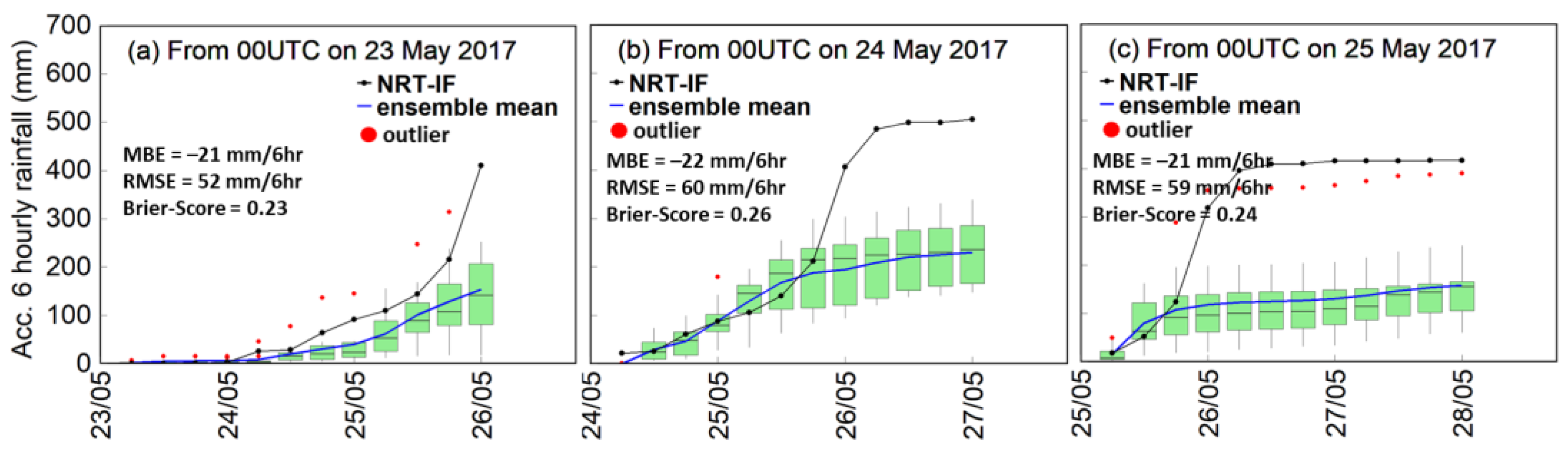
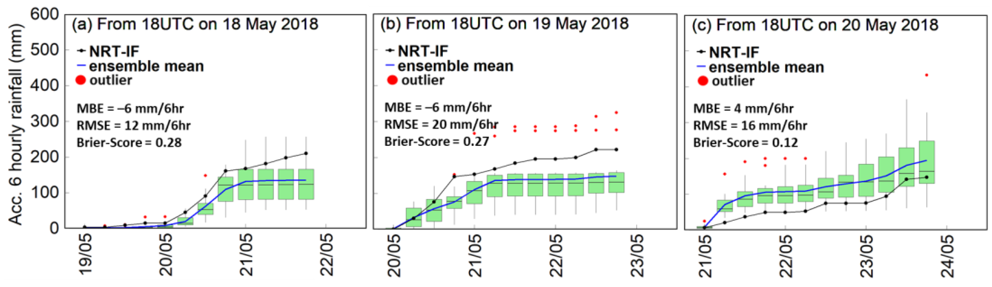
4.1.2. Ensemble Rainfall Forecasts

Figure 10a–c shows box-and-whisker plots to compare the basin-averaged ensemble rainfall spread and mean from the accumulated 6-hourly forecasts with NRT-IF data for the 72-h forecasting time starting at 00 UTC on 23, 24, and 25 May 2017. The error statistics (i.e., MBE and RMSE) of the ensemble mean and the Brier Score (BS) of the ensemble forecasts are given in the same figures. As shown in Figure 10a, the mean forecasts matched the NRT-IF data for the first 24 h; however, the forecasts were underestimated during the next 36 h, thus resulting in the underestimation of the mean (MBE = −21 mm/6 h and RMSE = 52 mm/6 h). Similarly, the mean forecasts on 24 May and 25 May matched the NRT-IF data for the first 36 and 18 h, respectively; however, those forecasts underestimated the peak rainfall intensities afterward, as shown in Figure 10b,c. Exceptionally, an ensemble member forecasted the peak intensities, as recorded by NRT-IF, but they fell outside the plotting range (i.e., 1.5 times the interquartile range) and were plotted as outliers in the figure. The estimated BS for ensemble rainfall amounts greater than 10 mm/6 h was found to be ~0.23–0.26 (a model with the perfect skill has a score of 0, and the worst has a score of 1) for all three cases, indicating the relatively good performance of the rainfall forecasts.

As shown in Figure 11a,b, unlike the forecasts for the May 2017 case, the mean forecast for the May 2018 case was relatively better with a slight underestimation (MBE = −6 mm/6 h, RMSE = ~12–20 mm/6 h) and coincided well with the timing of the observed peak rainfall during the first two days of the 72-h forecasting. The mean forecast on 20 May 2018, showed an overestimation of heavy rainfall events, as in Figure 11c. The BS of 0.12 for the forecasts on May 20 was relatively better compared to the previous forecasts on 18 May and 19 May 2018 (BS ~0.28).

4.2. Comparison of Hydrological Simulations and Forecasts of River Discharges

4.2.1. Hydrological Simulations Driven by GSMaP Products

Figure 12a compares the discharge driven by GSMaP products with observation at the Putupaula gauging station for the May 2017 flood event. The discharge data driven by GSMaP-NOW delayed the flood onset and underestimated the flood peak due to an underestimation of rainfall on 24 May and in the early hours of 25 May (Figure 6a,b). However, NOW-IF improved the timing of the flood onset, though it still underestimated the peak discharge rate compared to the observed discharge. The improvements in Nash and RMSE for NOW-IF data are significant; Nash improved from 0.76 to 0.97, and RMSE from 362.64 m³/s to 123.53 m³/s (

Table 3. Statistical metrics for the performance of the GSMaP products-derived discharge during 2017 and 2018 flood events.

Event	Errors (Units)	Discharge Derived from GSMaP Products
		NRT	NRT-IF	NOW	NOW-IF
	Nash–Sutcliffe Efficiency (-)	0.98	0.99	0.77	0.97
May 2017	RMSE (m3/s)	80.90	80.02	357.42	118.51
	MBE (m3/s)	−16.34	34.91	−226.88	−54.79
	Nash–Sutcliffe Efficiency (-)	0.50	0.93	0.26	0.87
May 2018	RMSE (m3/s)	300.34	109.57	363.79	150.24
	MBE (m3/s)	−200.40	12.71	−245.47	−52.65

). Furthermore, the hydrograph driven by GSMaP-NRT matched the observed one (Nash = 0.98), and the NRT-IF data improved the simulated hydrograph further (Nash = 0.99). Similarly, as shown in Figure 12b, the discharges driven by both GSMaP-NOW (Nash = 0.26) and GSMaP-NRT (Nash = 0.5) were underestimated due to the underestimation of rainfall during the early hours of the May 2018 case (Figure 7b). As expected, the discharges driven by the NRT-IF data (Nash = 0.93) were better than those driven by the NOW-IF data (Nash = 0.87).

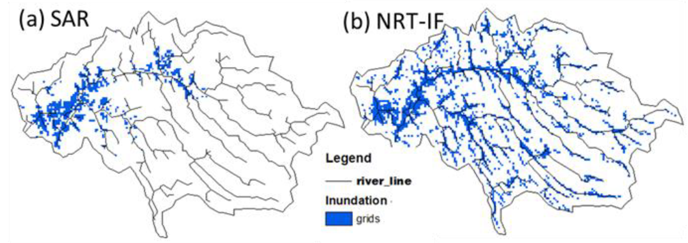
4.2.2. Inundation Extents Driven by the GSMaP Products

The maximum inundation depths (>1 m) driven by NRT-IF data were obtained from WEB-RRI model simulations and compared with satellite (SAR)-derived inundation extents for the May 2017 flood event. As shown in Figure 13a, the SAR data obtained on May 30, 2017 (~2 days after the peak flow) showed flood inundation mostly in the downstream flat regions, whereas the model showed inundation covering wider regions, including the upstream parts of the basins (Figure 13b), which were missed by the SAR data due to a late over-pass time and a faster flood travel time. Therefore, the model inundation information is useful for early warning and mitigation activities in the upstream regions. The estimated fit index (FI) and correctness index (CI) between the SAR data and the model-simulated inundation data were ~0.20 and ~0.64, respectively. Though there were significant differences in the bias-corrected rainfall amounts and simulated discharges between the NRT-IF and NOW-IF (not shown), the flood extent driven by the NOW-IF data was very similar (FI = 0.20 and CI = 0.59) to the NRT-IF data due to the simulated peak discharges (~2000 m³/s), which were well above the danger level (~1400 m³/s), as shown in Figure 12a.

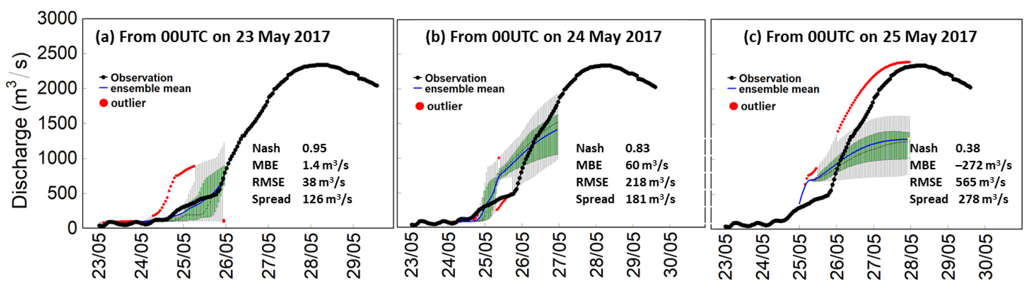
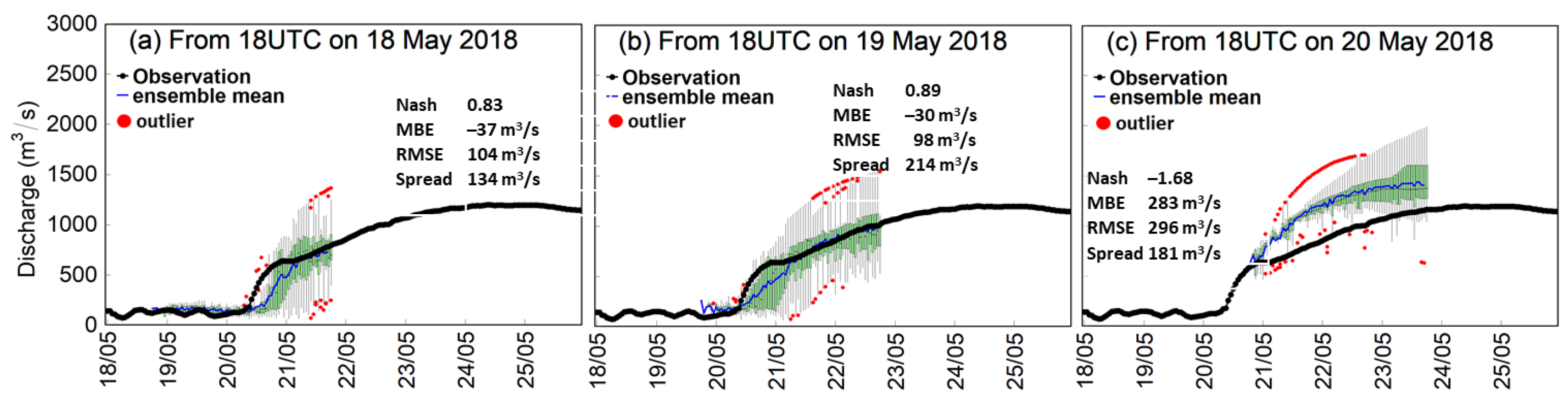
4.2.3. Hydrological Forecasts Driven by the Ensemble Rainfall Forecasts

Figure 14a–c compares the discharges driven by the rainfall forecasts with the observations at the Putupaula station for different forecasting times starting from 00 UTC on 23 May, 24 May, and 25 May 2017, respectively. As shown in Figure 14a,b, the mean discharges derived from the 23 and 24 May forecasts matched the observed discharges well. Particularly, the mean flow forecasts on 24 May predicted the peak flow conditions ~1400 m³/s (above the minor level), and the ensemble members above the 75-percentile predicted the peak discharges to be above 1500 m³/s. In the case of the discharge forecasting on 25 May (Figure 14c), the ensemble members below the 75th percentile failed to predict the peak flow condition due to the underestimation of rainfall forecasts (Figure 10c). Exceptionally, an ensemble member that forecast the peak rainfall in Figure 10c produced peak discharges comparable to the observed peak and tendency, though it was an outlier.

In the case of the May 2018 flood, as depicted in Figure 15a,b, the ensemble mean forecast matched the observed discharges well (Nash = ~0.8, RMSE = ~100 m³/s) since the forecasted rainfall intensities and their timings matched the observations reasonably well (Figure 11a,b). However, the mean flow forecast was overestimated on 20 May 2018 (Figure 15c) due to the overestimation of the mean rainfall forecast (Figure 11c). The time-averaged spread of the ensemble forecasts ranges from 134 m³/s to 214 m³/s for these flood events, as given in the same figures.

5. Discussions

The results showed that the GSMaP data can detect heavy rainfall events very well, but the intensities need to be adjusted using ground references to maximize their utilization for real-time applications. Particularly, the GSMaP-NRT data outperformed the GSMaP-NOW data in rainfall intensity and spatial distribution for both flood events, and thus the former is suitable for near-real-time flood-related applications. Though GSMaP-NOW is the preferred data source for real-time flood forecasting applications due to a shorter latency time, its quality is lower compared to GSMaP-NRT because of the limited microwave data availability and errors associated with extrapolation (which might have resulted in the shift in the rainfall location) using a backward-and-forward morphing technique and a Kalman filter for estimating precipitation [26,53,54]. Further improvements in the retrieval/interpolation techniques and incorporation of additional microwave data from upcoming satellite missions (e.g., Aerosol and Cloud, Convection, and Precipitation (ACCP)) [66] can enhance the performance of GSMaP-NOW products for real-time flood applications.

Previous studies in different river basins have demonstrated the good performance of GSMaP data in simulating peak river flow and inundation extents [67,68]. This study also showed that the streamflow simulations driven by satellite rainfall products can be used effectively for flood-related applications by combining them with limited real-time ground observations. The reason for obtaining good Nash values for discharge simulations (>0.9) in this study is the use of the WEB-RRI model, which eliminates model-related biases originating from the estimation of evapotranspiration and soil moisture dynamics [48]. Moreover, this study also confirmed that bias-corrected GSMaP-NOW (not investigated in the previous studies) and GSMaP-NRT data can be employed to prepare real-time rapid inundation maps for better flood management in early warning, rescue, and mitigation.

This study showed that the mean flow forecasts for both the May 2017 and May 2018 cases predicted the tendency of future flooding conditions reasonably well, therefore suggesting that these forecasts are useful for forecasting flood conditions with a reasonable lead time. A few studies have investigated the performance of ensemble rainfall and streamflow forecasts in selected flood events. Ushiyama et al. (2016) [69] found that the ensemble forecasting system could predict the probability of flood occurrence, though there were uncertainties in flood peaks and their timings. Sayama et al. (2020) [15] found that the actual peak runoff could not be well forecasted due to the uncertainties in the storm positions, and Magnusson et al. (2013) [70] pointed out that it was due to uncertainties in the initial conditions, which were generated from limited data collected from many parts of the world. Our experiments also identified two similar cases (i.e., a storm position shift in the May 2017 flood event and a false alarm after the May 2018 flood event). In the case of the May 2017 event, the storm position slightly shifted to the eastern side of the basin (Figure 16(b1)) compared to the NRT-IF data (Figure 16(a1)). In the case of the May 2018 heavy rainfall false alarm (Figure 16(b2)), heavy rainfall was captured by satellite rainfall estimates but was ~100 km away from the basin, as in Figure 16(a2). A detailed investigation will be performed in future studies.

6. Conclusions

This research proposed a basin-scale IFIS and investigated the performance of its major components by integrating multi-platform data from present-day ground and satellite observation techniques and numerical models for the recent flood events (i.e., a historical flood in May 2017 and a minor flood in May 2018) in the Kalu River basin, Sri Lanka.

The results of real-time and near-real-time GSMaP products revealed that both products deducted the heavy rainfall events well; however, GSMaP-NRT (4-h latency) outperformed GSMaP-NOW (0-h latency), which underestimated heavy rainfall events and showed a shift in the rainfall distribution that could be due to the interpolation of microwave data in unobserved regions by satellites within the shortest observation window. The merging of real-time gauge data with GSMaP data significantly improved the performance of both GSMaP products in rainfall intensity and distribution, flood event onset, and peak discharge estimations. The ensemble forecasts showed that the alarming signals of heavy rainfall were forecasted for both flood events, yet there were uncertainties in the forecasted rainfall amounts, locations, and timings. The bias or mismatch in storm positions was found to be a reason for the low performance of the rainfall forecasts. Despite significant uncertainties in the forecasted rainfall intensities and their timings, the river discharges driven by those forecasts showed strong signals in predicting flood peaks. Information on heavy rainfall, associated flood signals, and their possible range of probabilities from the system components is promising and helpful for flood-related activities in developing countries.

The demonstrated prototype system is currently in test operation in the Kalu River basin. Efforts are underway to develop and implement a similar system in other countries through the International Flood Initiative (IFI) of the World Meteorological Organization (WMO), and use this system for enhancing the capacity and technical knowledge of experts and policy-makers and eventually contribute to the UN initiative of “Early Warning for All within five years (2023–2027)”.

References

1. Hirabayashi, Y.; Mahendran, R.; Koirala, S.; Konoshima, L.; Yamazaki, D.; Watanabe, S.; Kim, H.; Kanae, S. Global flood risk under climate change. Nat. Clim. Chang. 2013, 3, 816–821. [Google Scholar] [CrossRef]
2. IPCC. The Physical Science Basis. Contribution of Working Group I to the Sixth Assessment Report of the Intergovernmental Panel on Climate Change; Cambridge University Press: Cambridge, UK; New York, NY, USA, 2021; p. 2391. [Google Scholar] [CrossRef]
3. Winsemius, H.C. Global drivers of future river flood risk. Nat. Clim. Chang. 2015, 6, 381–385. [Google Scholar] [CrossRef] [Green Version]
4. United Nations International Strategy for Disaster Reduction (UNISDR). Economic Losses, Poverty and Disasters: 1998–2017; ISDR: Geneva, Switzerland, 2018; p. 31. Available online: https://www.unisdr.org/files/61119_credeconomiclosses.pdf (accessed on 12 March 2023).
5. Perera, D.; Seidou, O.; Agnihotri, J.; Mehmood, H.; Rasmy, M. Challenges and Technical Advances in Flood Early Warning Systems (FEWSs), in Flood Impact Mitigation and Resilience Enhancement; IntechOpen: London, UK, 2020; Available online: https://www.intechopen.com/chapters/72571 (accessed on 12 March 2023).
6. UN Early Warning Action Plan at COP27. Available online: https://public.wmo.int/en/media/press-release/early-warnings-all-action-plan-unveiled-cop27 (accessed on 12 March 2023).
7. Sanchez Lozano, J.; Romero Bustamante, G.; Hales, R.C.; Nelson, E.J.; Williams, G.P.; Ames, D.P.; Jones, N.L. A Streamflow Bias Correction and Performance Evaluation Web Application for GEOGloWS ECMWF Streamflow Services. Hydrology 2021, 8, 71. [Google Scholar] [CrossRef]
8. Werner, M.; Schellekens, J.; Gijsbers, P.; van Dijk, M.; van den Akker, O.; Heynert, K. The Delft-FEWS flow forecasting system. Environ. Modell. Softw. 2012, 40, 65–77. [Google Scholar] [CrossRef] [Green Version]
9. Alfieri, L.; Burek, P.; Dutra, E.; Krzeminski, B.; Muraro, D.; Thielen, J.; Pappenberger, F. GloFAS-global ensemble streamflow forecasting and flood early warning. Hydrol. Earth Syst. Sci. 2013, 17, 1161–1175. [Google Scholar] [CrossRef] [Green Version]
10. Lavers, D.A.; Harrigan, S.; Andersson, E.; Richardson, D.S.; Prudhomme, C.; Pappenberger, F. A vision for improving global flood forecasting. Environ. Res. Lett. 2019, 14, 121002. [Google Scholar] [CrossRef] [Green Version]
11. Demargne, J.; Wu, L.; Regonda, S.K.; Brown, J.D.; Lee, H.; He, M.; Seo, D.-J.; Hartman, R.; Herr, H.D.; Fresch, M.; et al. The science of NOAA’s operational hydrologic ensemble forecast service. Bull. Am. Meteorol. Soc. 2014, 95, 79–98. [Google Scholar] [CrossRef]
12. Thielen, J.; Bartholmes, J.; Ramos, M.H.; de Roo, A. The European Flood Alert System—Part 1: Concept and development. Hydrol. Earth Syst. Sci. 2009, 13, 125–140. [Google Scholar] [CrossRef] [Green Version]
13. Bartholmes, J.C.; Thielen, J.; Ramos, M.H.; Gentilini, S. The European flood alert system EFAS Part 2: Statistical skill assessment of probabilistic and deterministic operational forecasts. Hydrol. Earth Syst. Sci. 2009, 13, 141–153. [Google Scholar] [CrossRef] [Green Version]
14. Emerton, R.E.; Stephens, E.M.; Pappenberger, F.; Pagano, T.C.; Weerts, A.H.; Wood, A.W.; Salamon, P.; Brown, J.D.; Hjerdt, N.; Donnelly, C.; et al. Continental and global scale flood forecasting systems. Wiley Interdiscip. Rev. Water 2016, 3, 391–418. [Google Scholar] [CrossRef] [Green Version]
15. Sayama, T.; Yamada, M.; Sugawara, Y.; Yamazaki, D. Ensemble flash flood predictions using a high-resolution nationwide distributed rainfall-runoff model: Case study of the heavy rain event of July 2018 and Typhoon Hagibis in 2019. Prog. Earth Planet Sci. 2020, 7, 75. [Google Scholar] [CrossRef]
16. Ma, W.; Ishitsuka, Y.; Takeshima, A.; Hibino, K.; Yamazaki, D.; Yamamoto, K.; Kachi, M.; Oki, R.; Oki, T.; Yoshimura, K. Applicability of a nationwide flood forecasting system for Typhoon Hagibis 2019. Sci. Rep. 2021, 11, 10213. [Google Scholar] [CrossRef] [PubMed]
17. Hoedjes, J.C.B.; Kooiman, A.; Maathuis, B.H.P.; Said, M.Y.; Becht, R.; Limo, A.; Mumo, M.; Nduhiu-Mathenge, J.; Shaka, A.; Su, B. A Conceptual Flash Flood Early Warning System for Africa, Based on Terrestrial Microwave Links and Flash Flood Guidance. ISPRS Int. J. Geo-Inf. 2014, 3, 584–598. [Google Scholar] [CrossRef] [Green Version]
18. Chitwatkulsiri, D.; Miyamoto, H.; Irvine, K.N.; Pilailar, S.; Loc, H.H. Development and Application of a Real-Time Flood Forecasting System (RTFlood System) in a Tropical Urban Area: A Case Study of Ramkhamhaeng Polder, Bangkok, Thailand. Water 2022, 14, 1641. [Google Scholar] [CrossRef]
19. Manzoor, Z.; Ehsan, M.; Khan, M.B.; Manzoor, A.; Akhter, M.M.; Sohail, M.T.; Hussain, A.; Shafi, A.; Abu-Alam, T.; Abioui, M. Floods and flood management and its socio-economic impact on Pakistan: A review of the empirical literature. Front. Environ. Sci. 2022, 10, 1–14. [Google Scholar] [CrossRef]
20. Smith, P.J.; Brown, S.; Dugar, S. Community Based Early Warning Systems for flood risk mitigation in Nepal. Nat. Hazards Earth Syst. Sci. 2017, 17, 423–437. [Google Scholar] [CrossRef] [Green Version]
21. Sai, F.; Cumiskey, L.; Weerts, A.; Bhattacharya, B.; Khan, R. Towards impact-based flood forecasting and warning in Bangladesh: A case study at the local level in Sirajganj district. Nat. Hazards Earth Syst. Sci. Discuss. 2018, 2018, 1–20. [Google Scholar] [CrossRef]
22. Nanditha, J.; Mishra, V. On the need of ensemble flood forecast in India. Water Secur. 2021, 12, 100086. [Google Scholar] [CrossRef]
23. Tan, J.; Petersen, W.A.; Kirstetter, P.E.; Tian, Y. Performance of IMERG as a function of spatiotemporal scale. J. Hydrometeorol. 2017, 18, 307–319. [Google Scholar] [CrossRef]
24. Skofronick-Jackson, G.; Kirschbaum, D.; Petersen, W.; Huffman, G.; Kidd, C.; Stocker, E.; Kakar, R. The Global Precipitation Measurement (GPM) mission’s scientific achievements and societal contributions: Reviewing four years of advanced rain and snow observations. Quart. J. Roy. Meteor. Soc. 2018, 144, 27–48. [Google Scholar] [CrossRef] [Green Version]
25. Huffman, G.J.; Bolvin, D.T.; Braithwaite, D.; Hsu, K.; Joyce, R.; Kidd, C.; Nelkin, E.J.; Sorooshian, S.; Tan, J.; Xie, P. Algorithm Theoretical Basis Document (ATBD) Version 5.2 for the NASA Global Precipitation Measurement (GPM) Integrated Multi-satellitE Retrievals for GPM (I-MERG); GPM Project 2019; NASA: Greenbelt, MD, USA, 2019; p. 38. Available online: https://gpm.nasa.gov/sites/default/files/document_files/IMERG_ATBD_V06.pdf (accessed on 12 March 2023).
26. Kubota, T.; Aonashi, K.; Ushio, T.; Shige, S.; Takayabu, Y.N.; Kachi, M.; Arai, Y.; Tashima, T.; Masaki, T.; Kawamoto, N.; et al. Global Satellite Mapping of Precipitation (GSMaP) Products in the GPM Era. In Satellite Precipitation Measurement. Advances in Global Change Research; Levizzani, V., Kidd, C., Kirschbaum, D., Kummerow, C., Nakamura, K., Turk, F., Eds.; Springer: Cham, Switzerland, 2020; Volume 67, pp. 355–373. [Google Scholar]
27. Khairul, I.M.; Mastrantonas, N.; Rasmy, M.; Koike, T.; Takeuchi, K. Inter-Comparison of Gauge-Corrected Global Satellite Rainfall Estimates and Their Applicability for Effective Water Resource Management in a Transboundary River Basin: The Case of the Meghna River Basin. Remote Sens. 2018, 10, 828. [Google Scholar] [CrossRef] [Green Version]
28. Mastrantonas, N.; Bhattacharya, B.; Shibuo, Y.; Rasmy, M.; Espinoza-Dávalos, G.; Solomatine, D. Evaluating the Benefits of Merging Near-Real-Time Satellite Precipitation Products: A Case Study in the Kinu Basin Region, Japan. J. Hydrometeorol. 2019, 20, 1213–1233. [Google Scholar] [CrossRef]
29. Tashima, T.; Kubota, T.; Mega, T.; Ushio, T.; Oki, R. Precipitation extremes monitoring using the near-real-time GSMaP product. Remote Sens. 2020, 13, 5640–5651. [Google Scholar] [CrossRef]
30. Zhou, L.; Rasmy, M.; Takeuchi, K.; Koike, T.; Selvarajah, H.; Ao, T. Adequacy of Near-Real-Time Satellite Precipitation Products in Driving Flood Discharge Simulation in the Fuji River Basin, Japan. Appl. Sci. 2021, 11, 1087. [Google Scholar] [CrossRef]
31. Zhou, L.; Koike, T.; Takeuchi, K.; Rasmy, M.; Onuma, K.; Ito, H.; Selvarajah, H.; Liu, L.; Li, X.; Ao, T. A Study on Availability of Ground Observations and Its Impacts on Bias Correction of Satellite Precipitation Products and Hydrologic Simulation Efficiency. J. Hydrol. 2022, 310, 127595. [Google Scholar] [CrossRef]
32. Cloke, H.L.; Pappenberger, F. Ensemble flood forecasting: A review. J. Hydrol. 2009, 375, 613–626. [Google Scholar] [CrossRef]
33. Webster, P.J.; Jian, J.; Hopson, T.M.; Hoyos, C.D.; Agudelo, P.A.; Chang, H.-R.; Curry, J.A.; Grossman, R.L.; Palmer, T.; Subbiah, A.R. Extended-Range Probabilistic Forecasts of Ganges and Brahmaputra Floods in Bangladesh. Bull. Am. Meteorol. Soc. 2010, 91, 1493–1514. [Google Scholar] [CrossRef] [Green Version]
34. Cuo, L.; Pagano, T.C.; Wang, Q.J. A review of quantitative precipitation forecasts and their use in short- to medium-range streamflow forecasting. J. Hydrometeorol. 2011, 12, 713–728. [Google Scholar] [CrossRef]
35. Ushiyama, T.; Sayama, T.; Tatebe, Y.; Fujioka, S.; Fukami, K. Numerical Simulation of 2010 Pakistan Flood in the Kabul River Basin by Using Lagged Ensemble Rainfall Forecasting. J. Hydrometeorol. 2014, 15, 193–211. Available online: http://www.jstor.org/stable/24914368 (accessed on 12 March 2023). [CrossRef]
36. Bowler, N.; Arribas, A.; Mylne, K.; Robertson, K.; Beare, S. The MOGREPS short-range ensemble prediction system. Q. J. R. Meteorol. Soc. 2008, 134, 703–722. [Google Scholar] [CrossRef]
37. Molteni, F.R.; Buizza, R.; Palmer, T.N.; Petroliagis, T. The ECMWF Ensemble Prediction System: Methodology and validation. Q. J. R. Meteorol. Soc. 1996, 122, 73–119. [Google Scholar] [CrossRef]
38. Toth, Z.; Kalnay, E. Ensemble forecasting at NCEP and the breeding method. Mon. Weather Rev. 1997, 125, 3297–3319. [Google Scholar] [CrossRef]
39. Wu, W.; Emerton, R.; Duan, Q.; Wood, A.W.; Wetterhall, F.; Robertson, D.E. Ensemble flood forecasting: Current status and future opportunities. Wiley Interdiscip. Rev. Water 2020, 62, e1432. [Google Scholar] [CrossRef]
40. Ho, J.-Y.; Liu, C.-H.; Chen, W.-B.; Chang, C.-H.; Lee, K.T. Using ensemble quantitative precipitation forecast for rainfall-induced shallow landslide predictions. Geosci. Lett. 2022, 9, 22. [Google Scholar] [CrossRef]
41. Chessa, P.A.; Lalaurette, F. Verification of the ECMWF Ensemble Prediction System Forecasts: A Study of Large-scale Patterns. Weather. Forecast. 2001, 16, 611–619. [Google Scholar] [CrossRef]
42. Vegad, U.; Mishra, V. Ensemble streamflow prediction considering the influence of reservoirs in Narmada River Basin, India. Hydrol. Earth Syst. Sci. 2022, 26, 6361–6378. [Google Scholar] [CrossRef]
43. Patel, A.; Yadav, S.M. Stream flow prediction using TIGGE ensemble precipitation forecast data for Sabarmati river basin. Water Supply 2022, 22, 8317–8336. [Google Scholar] [CrossRef]
44. Manikanta, V.; Nikhil Teja, K.; Das, J.; Umamahesh, N. On the verification of ensemble precipitation forecasts over the Godavari River basin. J. Hydrol. 2023, 616, 128794. [Google Scholar] [CrossRef]
45. Van der Knijff, J.; Younis, J.; de Roo, A. LISFLOOD: A GIS-based distributed model for river basin scale water balance and flood simulation. Int. J. Geogr. Inf. Sci. 2010, 24, 189–212. [Google Scholar] [CrossRef]
46. Yamazaki, D.; Sato, T.; Kanae, S.; Hirabayashi, Y.; Bates, P.D. Regional flood dynamics in a bifurcating mega delta simulated in a global river model. Geophys. Res. Lett. 2014, 41, 3127–3135. [Google Scholar] [CrossRef] [Green Version]
47. Sayama, T.; Ozawa, G.; Kawakami, T.; Nabesaka, S.; Fukami, K. Rainfall-Runoff-Inundation Analysis of Pakistan Flood 2010 at the Kabul River Basin. Hydrol. Sci. J. 2012, 57, 298–312. [Google Scholar] [CrossRef]
48. Rasmy, M.; Sayama, T.; Koike, T. Development of Water and Energy Budget-Based Rainfall-Runoff-Inundation Model (WEB-RRI) and Its Verification in the Kalu and Mundeni River Basins, Sri Lanka. J. Hydrol. 2019, 579, 124163. [Google Scholar] [CrossRef]
49. Nandalal, K.D.W. Use of a hydrodynamic model to forecast floods of Kalu River in Sri Lanka. J. Flood Risk Manag. 2009, 2, 151–158. [Google Scholar] [CrossRef]
50. Kobayashi, S.; Ota, Y.; Harada, Y.; Ebita, A.; Moriya, M.; Onoda, H.; Onogi, K.; Kamahori, H.; Kobayashi, C.; Endo, H.; et al. The JRA-55 Reanalysis: General specifications and basic characteristics. J. Meteor. Soc. Jpn. 2015, 93, 5–48. [Google Scholar] [CrossRef] [Green Version]
51. Kubota, T.; Shige, S.; Hashizume, H.; Aonashi, K.; Takahashi, N.; Seto, S.; Hirose, M.; Takayabu, Y.N.; Ushio, T.; Nakagawa, K.; et al. Global precipitation map using satellite-borne microwave radiometers by the GSMaP project: Production and validation. IEEE Trans. Geosci. Remote Sens. 2007, 45, 2259–2275. [Google Scholar] [CrossRef]
52. Aonashi, K.; Awaka, J.; Hirose, M.; Kozu, T.; Kubota, T.; Liu, G.; Shige, S.; Kida, S.; Seto, S.; Takahashi, N.; et al. GSMaP passive, microwave precipitation retrieval algorithm: Algorithm description and validation. J. Meteor. Soc. Jpn. 2009, 87A, 119–13640. [Google Scholar] [CrossRef] [Green Version]
53. Joyce, R.J.; Janowiak, J.E.; Arkin, P.A.; Xie, P. CMORPH: A method that produces global precipitation estimates from passive microwave and infrared data at high spatial and temporal resolution. J. Hydrometeorol. 2004, 5, 487–503. [Google Scholar] [CrossRef]
54. Ushio, T.; Sasashige, K.; Kubota, T.; Shige, S.; Okamoto, K.; Aonashi, K.; Inoue, T.; Takahashi, N.; Iguchi, T.; Kachi, M.; et al. A Kalman filter approach to the Global Satellite Mapping of Precipitation (GSMaP) from combined passive microwave and infrared radiometric data. J. Meteorol. Soc. Jpn. 2009, 87A, 137–151. [Google Scholar] [CrossRef] [Green Version]
55. Chen, S.; Hu, J.; Zhang, A.; Min, C.; Huang, C.; Liang, Z. Performance of near real-time Global Satellite Mapping of Precipitation estimates during heavy precipitation events over northern China. Theor. Appl. Climatol. 2019, 135, 877–891. [Google Scholar] [CrossRef]
56. Skamarock, W.C.; Klemp, J.B.; Dudhia, J.; Gill, D.O.; Zhiquan, L.; Berner, J.; Wang, W.; Powers, J.G.; Duda, M.G.; Barker, D.M.; et al. A Description of the Advanced Research WRF Model Version 4; Technical Report NCAR/TN-475+STR for National Center for Atmospheric Research: Boulder, CO, USA, 2019. [Google Scholar] [CrossRef]
57. Zhou, X.; Zhu, Y.; Hou, D.; Luo, Y.; Peng, J.; Wobus, R. Performance of the New NCEP Global Ensemble Forecast System in a Parallel Experiment. Weather Forecast. 2017, 32, 1989–2004. [Google Scholar] [CrossRef]
58. Marsigli, C.; Boccanera, F.; Montani, A.; Paccagnella, T. The COSMO-LEPS mesoscale ensemble system: Validation of the methodology and verification. Nonlin. Process. Geophys. 2005, 12, 527–536. [Google Scholar] [CrossRef] [Green Version]
59. Lehner, B.; Verdin, K.; Jarvis, A. New global hydrography derived from spaceborne elevation data. Eos Trans. Am. Geophys. Union 2008, 89, 2. [Google Scholar] [CrossRef]
60. Sellers, P.J.; Tucker, C.J.; Collatz, G.J.; Los, S.; Justice, C.O.; Dazlich, D.A.; Randall, D. A revised land surface parameterization (SiB2) for atmospheric GCMs, Part I: Model formulation. J. Clim. 1996, 9, 676–705. [Google Scholar] [CrossRef]
61. Sellers, P.J.; Tucker, C.J.; Collatz, G.J.; Los, S.; Justice, C.O.; Dazlich, D.A.; Randall, D. A revised land surface parameterization (SiB2) for atmospheric GCMs, Part II: The generation of global fields of terrestrial biophysical parameters from satellite data. J. Clim. 1996, 9, 706–737. [Google Scholar] [CrossRef]
62. Wang, L.; Koike, T.; Yang, K.; Jackson, T.J.; Bindlish, R.; Yang, D. Development of a distributed biosphere hydrological model and its evaluation with the Southern Great Plains Experiments (SGP97 and SGP99). J. Geophys. Res. 2009, 114, D08107. [Google Scholar] [CrossRef] [Green Version]
63. Brier, G.W. Verification of forecasts expressed in terms of probability. Mon. Weather Rev. 1950, 78, 1–3. [Google Scholar] [CrossRef]
64. Bates, P.; De Roo, A. A simple raster-based model for flood inundation simulation. J. Hydrol. 2000, 236, 54–77. [Google Scholar] [CrossRef]
65. Liu, Z.; Merwade, V.; Jafarzadegan, K. Investigating the role of model structure and surface roughness in generating flood inundation extents using one- and two-dimensional hydraulic models. J. Flood Risk Manag. 2019, 12, e12347. [Google Scholar] [CrossRef] [Green Version]
66. Braun, S. Aerosol, Cloud, Convection, and Precipitation (ACCP) Science & Applications. March 2022. Available online: https://aos.gsfc.nasa.gov/docs/ACCP_Science_Narrative-(Mar2022).pdf (accessed on 22 July 2022).
67. Yoshimoto, S.; Amarnath, G. Applications of Satellite-Based Rainfall Estimates in Flood Inundation Modeling—A Case Study in Mundeni Aru River Basin, Sri Lanka. Remote Sens. 2017, 9, 998. [Google Scholar] [CrossRef] [Green Version]
68. Tam, T.H.; Abd Rahman, M.Z.; Harun, S.; Hanapi, M.N.; Kaoje, I.U. Application of Satellite Rainfall Products for Flood Inundation Modelling in Kelantan River Basin, Malaysia. Hydrology 2019, 6, 95. [Google Scholar] [CrossRef] [Green Version]
69. Ushiyama, T.; Sayama, T.; Iwami, Y. Ensemble Flood Forecasting of Typhoons Talas and Roke at Hiyoshi Dam Basin. J. Disaster Res. 2016, 11, 1032–1039. [Google Scholar] [CrossRef]
70. Magnusson, L.; Källén, E. Factors influencing skill improvements in the ECMWF forecasting system. Mon. Weather Rev. 2013, 141, 3142–3153. [Google Scholar] [CrossRef]
Figure 1. Locations of the study area and gauges: (a) the demarcation of the Kalu River basin, digital elevation model, and the river network and (b) annual GSMaP rainfall climatology (2001–2015) and the location of real-time rain gauges (green dots).
Water 15 01199 g001
Figure 2. Schematic diagram of the research framework for the real-time flood monitoring, forecasting, and early warning systems.
Water 15 01199 g002
Figure 3. Flow chart for the NTT-DATA GSMaP bias-correction algorithm.
Water 15 01199 g003
Figure 4. Model domains and topographical map used for numerical weather forecasting: (a) the outer domain at 20 km grid resolution and (b) the inner domain at 5 km grid resolution.
Water 15 01199 g004
Figure 5. Schematic diagram of the water and energy budget-based rainfall–runoff–inundation (WEB-RRI) model and its four major modules. Reprinted with permission from Ref. [48].
Water 15 01199 g005
Figure 6. Comparison of basin-averaged GSMaP raw and bias-corrected (IF) rainfall products for May 2017 event: (a) daily rainfall (mm/day) and (b) hourly rainfall (mm/h).
Water 15 01199 g006
Figure 7. Same as Figure 6 but for May 2018 event: (a) daily rainfall (mm/day) and (b) hourly rainfall (mm/h).
Water 15 01199 g007
Figure 8. Comparison of daily cumulative rainfall (mm/day) distributions on 25 May 2017 for (a) real-time ground data; (b) GSMaP-NOW; (c) GSMaP-NRT; (d) bias-corrected GSMaP-NOW (NOW-IF); and (e) bias-corrected GSMaP-NRT (NRT-IF).
Water 15 01199 g008
Figure 9. Comparison of daily cumulative rainfall (mm/day) distributions on 20 May 2018 for (a) real-time ground rainfall data; (b) GSMaP-NOW; (c) GSMaP-NRT; (d) bias-corrected GSMaP-NOW (NOW-IF); and (e) bias-corrected GSMaP-NRT (NRT-IF).
Water 15 01199 g009
Figure 10. Comparison of basin-averaged 6-hourly accumulated ensemble rainfall with GSMaP-NRT-IF for 2017 flood event starting from (a) 00 UTC on 23 May; (b) 00 UTC on 24 May; and (c) 00 UTC on 25 May 2017. The green boxes indicate the 25th and 75th percentile values of the ensemble forecasts, black middle bars are for the median, and vertical lines are for maximum and minimum values.
Water 15 01199 g010
Figure 11. Same as Figure 10 but for the 2018 flood event starting from (a) 18 UTC on 18 May; (b) 18 UTC on 19 May; and (c) 18 UTC on 10 May 2018.
Water 15 01199 g011
Figure 12. Comparison of model-simulated hourly discharges with observation discharges at Putupaula gauging station from (a) 21 May to 9 June 2017 and (b) 18 May to 3 June 2018.
Water 15 01199 g012
Figure 13. Comparison of flood inundation extents derived for the 2017 flood event in the Kalu River basin: (a) SAR and (b) NRT-IF.
Water 15 01199 g013
Figure 14. Comparison of model-simulated ensemble discharges with observation (m3/s) at the Putupaula gauging station for each forecasting time starting from 00 UTC on (a) 23 May, (b) 24 May, and (c) 25 May 2017.
Water 15 01199 g014
Figure 15. Same as Figure 14 but for each forecasting time starting from 18 UTC on (a) 18 May, (b) 19 May, and (c) 20 May 2018.
Water 15 01199 g015
Figure 16. Comparison of daily rainfall (mm/day) distributions: (a1) NRT-IF data for 25 May 2017; (b1) ensemble mean rainfall forecasted at 00 UTC on 24 May 2017 for 25 May 2017; (a2) NRT-IF data for 24 May 2018; and (b2) ensemble mean rainfall forecasted at 00 UTC on 23 May 2018 for 24 May 2018.
Water 15 01199 g016