
Estimating Land Subsidence and Gravimetric Anomaly Induced by Aquifer Overexploitation in the Chandigarh Tri-City Region, India by Coupling Remote Sensing with a Deep Learning Neural Network Model

Abstract
:1. Introduction
- Use freely available C-band Sentinel-1 SAR data-based PSInSAR for urban surface displacement mapping of Chandigarh tri-city region from 2017 to 2022, thus making the study cost-effective.
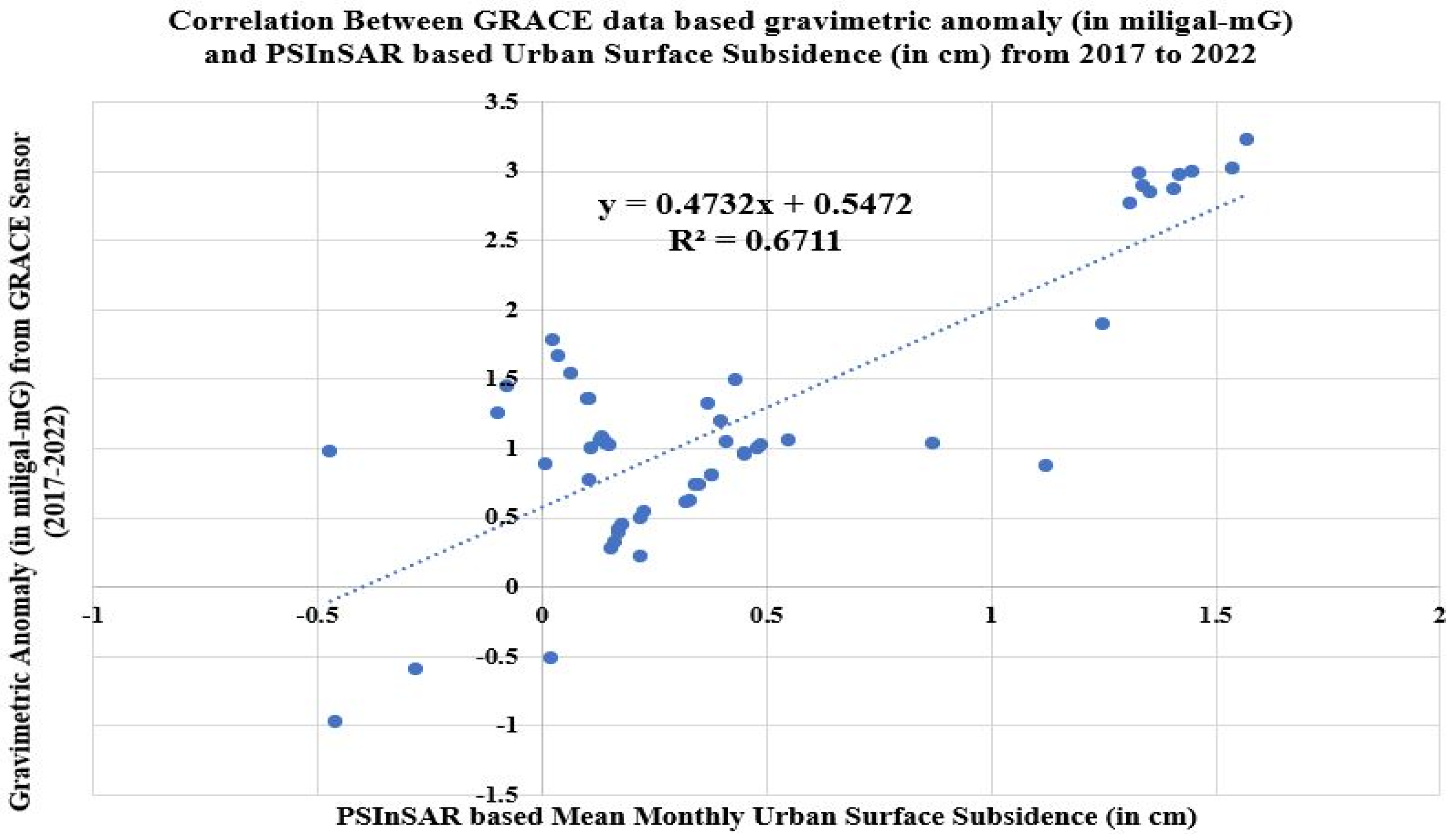
- Explore the interoperability of C-band SAR and GRACE gravimetric satellite sensors for groundwater exploitation-induced groundwater storage change.
- Estimate the groundwater storage at the city level using the DLMLP model and PSInSAR, groundwater data from wells, and GRACE data as parameters.
2. Materials and Methods
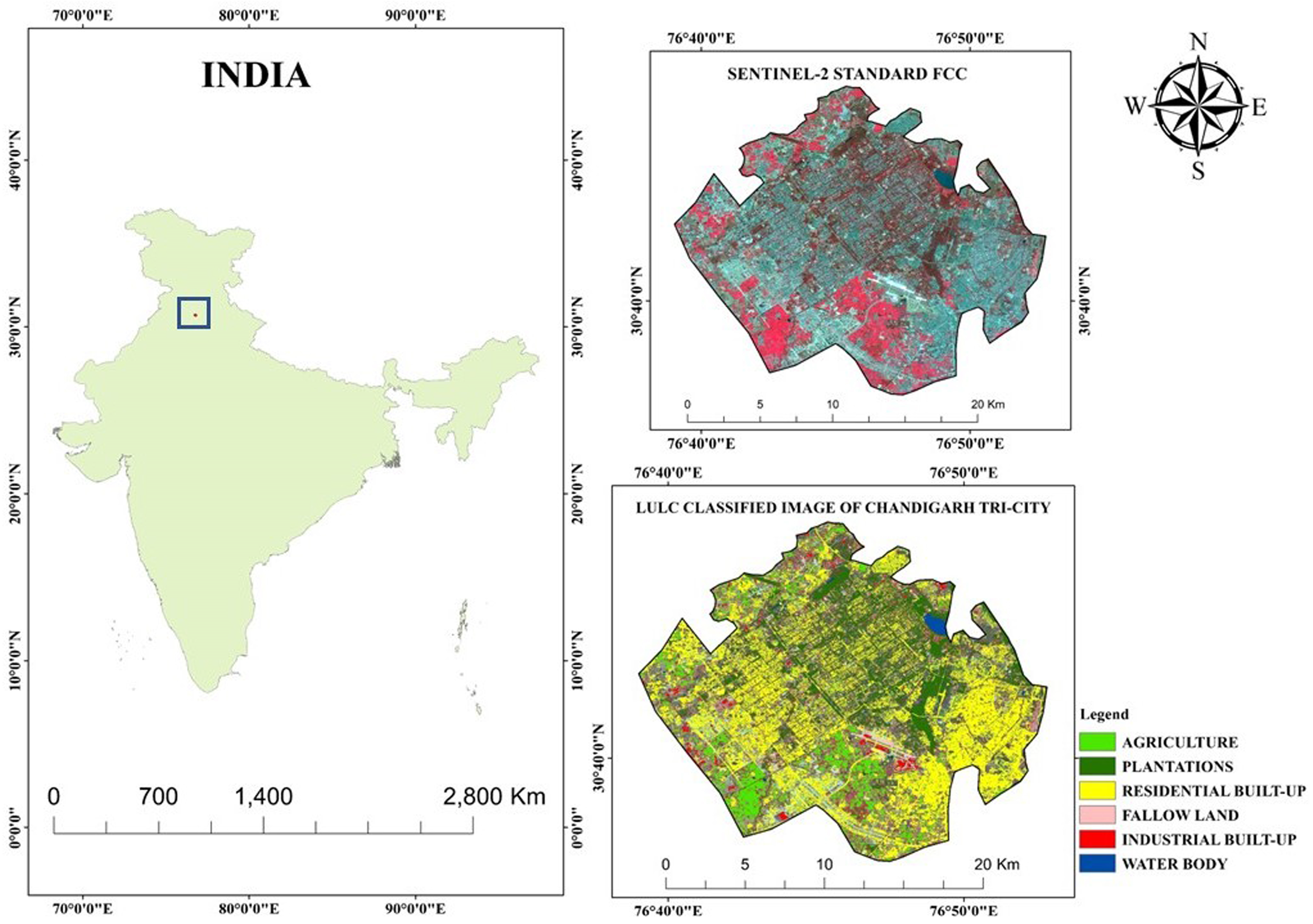
2.1. Study Area
2.2. Hydro Geology of Chandigarh Tri-City Region
2.3. Materials
2.4. Methods
2.4.1. SAR Data Pre-Processing
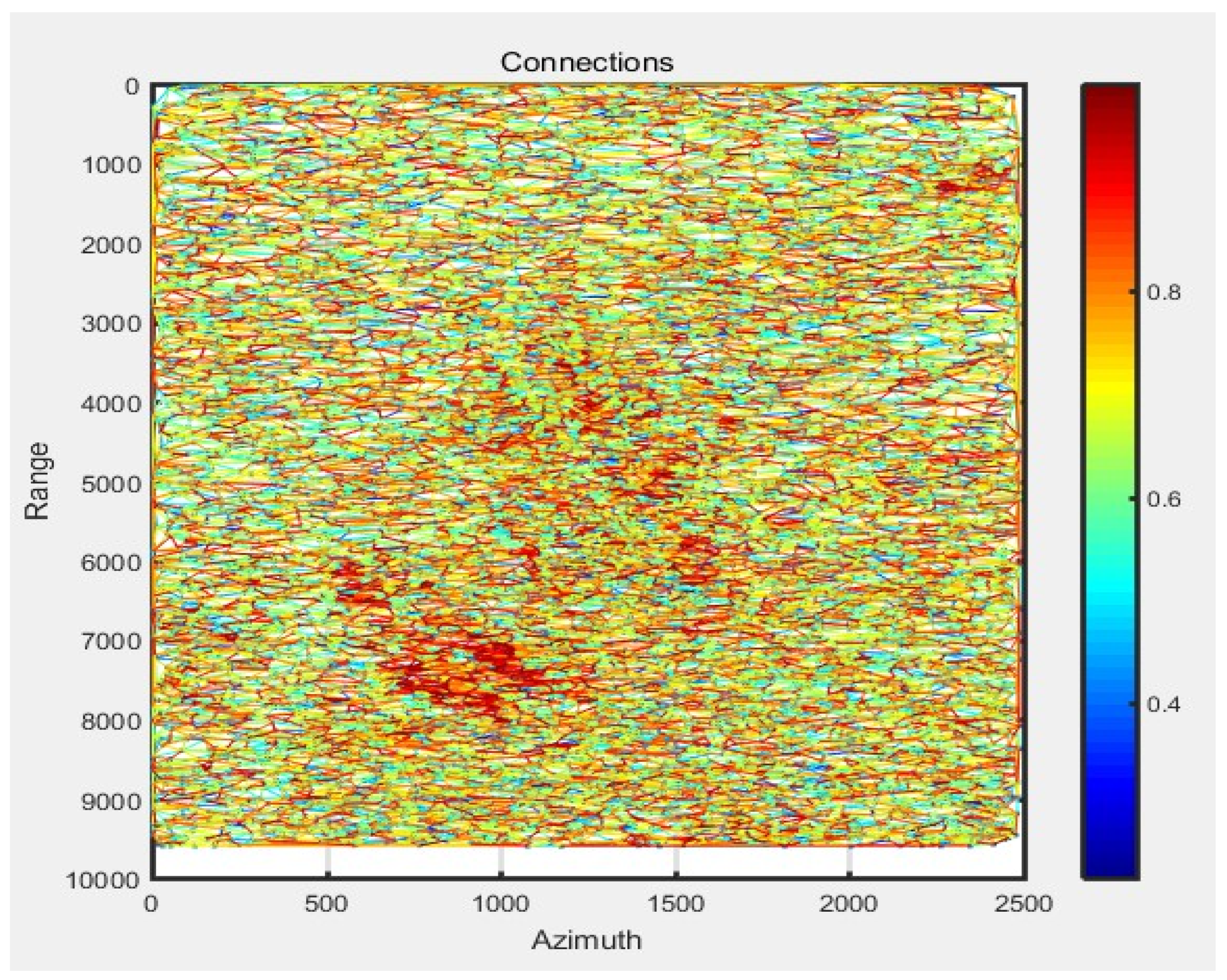
2.4.2. SAR Data Interferometric Processing
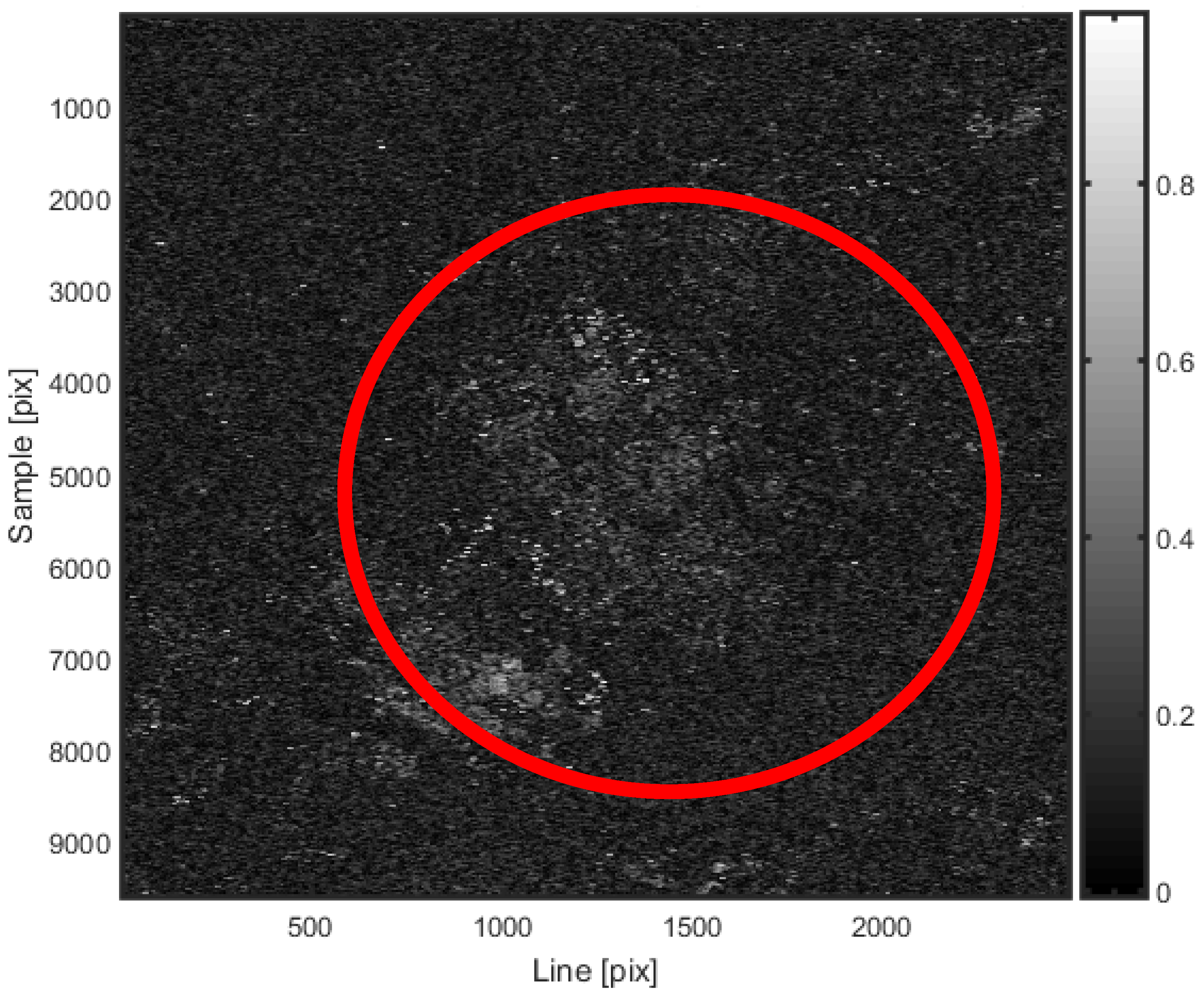
2.4.3. Atmospheric Phase Screen (APS) Removal
2.4.4. Time Series Analysis
2.4.5. GRACE Data Processing
2.4.6. Deep Learning Multi-Layer Perceptron (DLMLP) Model
3. Results


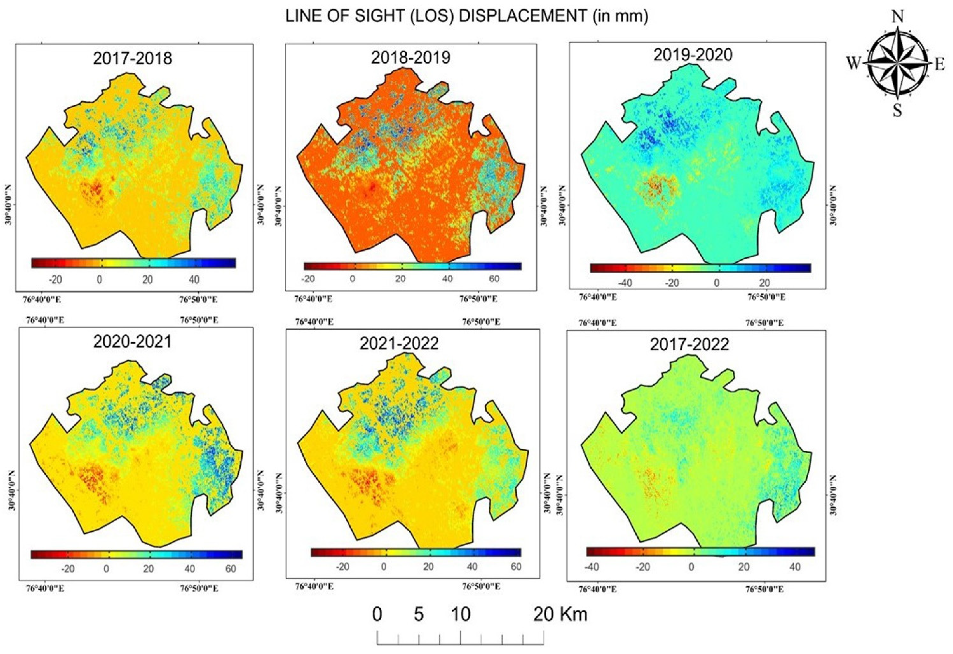
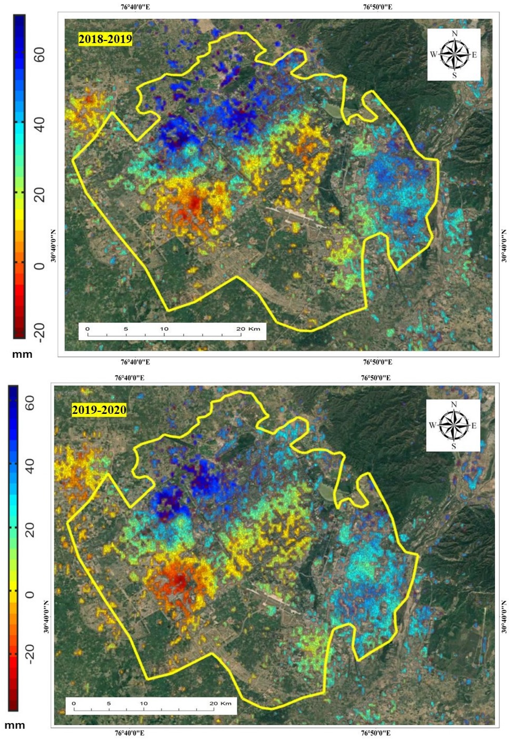
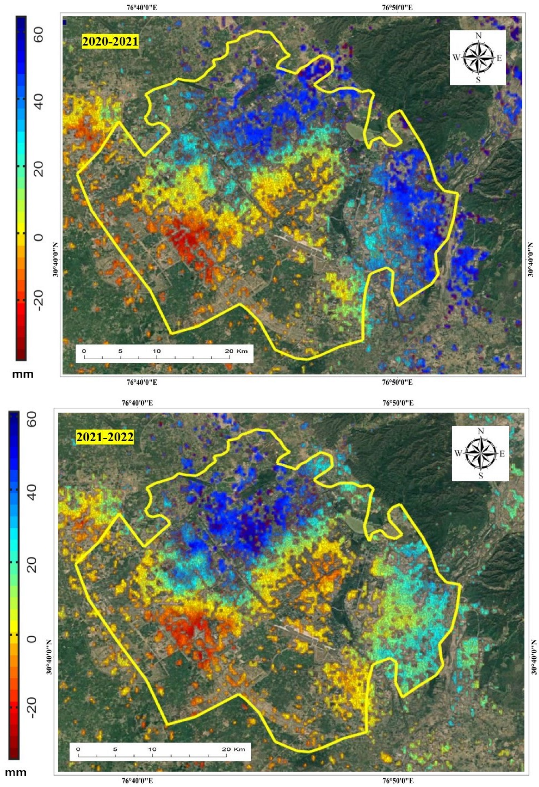
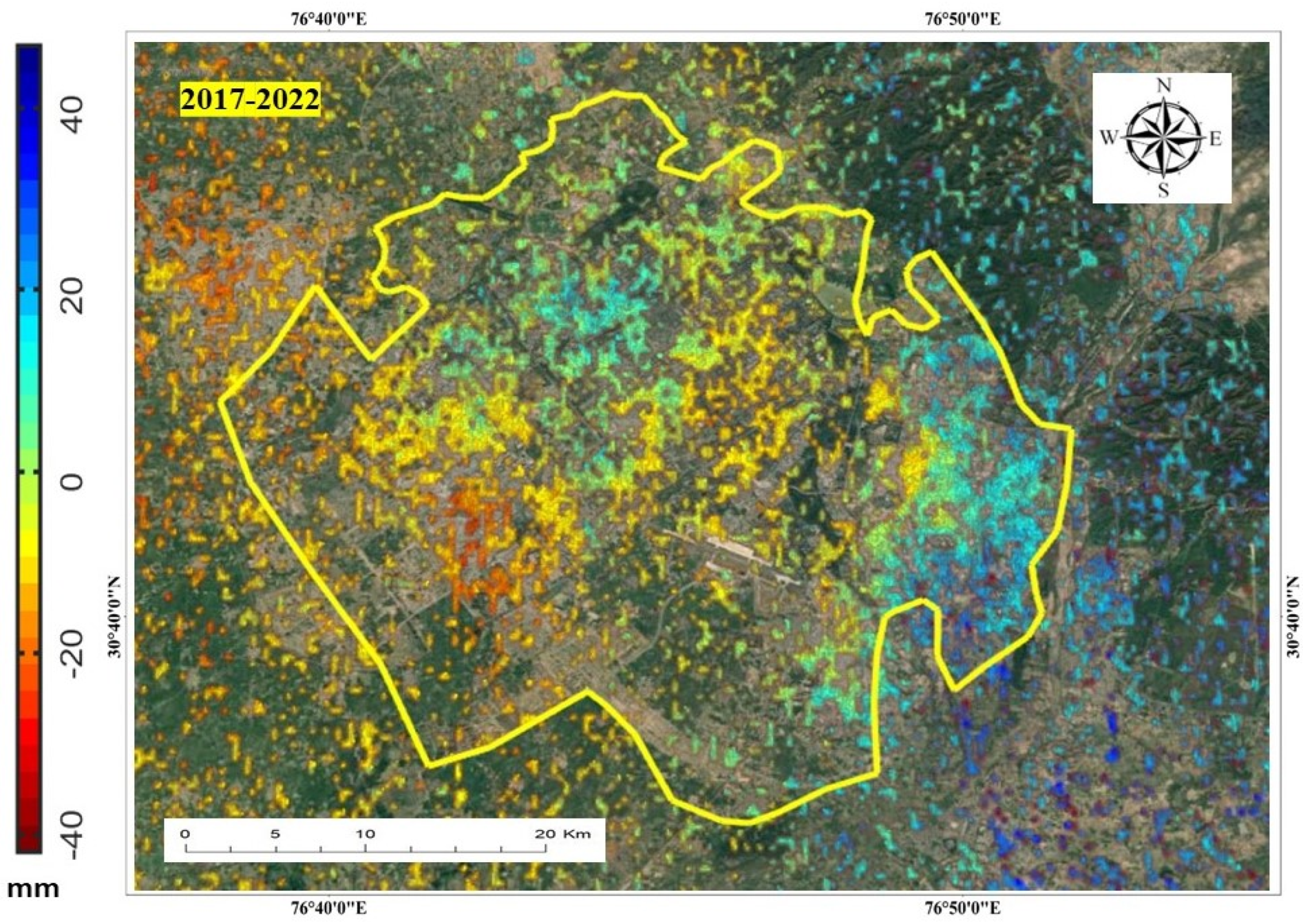
Time Series Analysis
4. Discussion
Points of Difference with a Previous Study by Tripathi et al. (2022) [46]
- Owing to a large amount of per pixel data and a detailed time series analysis for PSInSAR displacement, a more complex machine learning model (the DLMLP) has been used here.
- This study makes use of GLDAS-LSM data along with the GRACE and Sentinel-1 Satellite datasets.
- In the study conducted for Varanasi, the change in GRACE data values was an indicator of groundwater fluctuations, while in this study for Chandigarh, surface water has been subtracted to focus more precisely on the groundwater storage changes only.
- Both Varanasi and Chandigarh are different in their location and geology, as the city of Varanasi has newer alluvium, and still the mighty Ganges is a big source of water supply for the region. For Chandigarh, the situation is more complex since it entirely depends upon the groundwater to meet its water requirements; hence, this study is more crucial.
- The seismic risks are higher for Chandigarh and surface displacement is more crucial since Chandigarh is in seismic zone IV/V while Varanasi is in seismic zone III. Therefore, this study details the time series analysis more as compared to Varanasi (see Section 2.4.4).
5. Conclusions
- This study establishes that remotely sensed ΔGWS can be used as an indicator of groundwater depletion.
- The study proves that with the interoperability of SAR and GRACE sensors, regular monitoring of urban surface subsidence and ΔGWS can be carried out.
- The study also estimates city level ΔGWS using the interoperability of Sentinel-1 SAR and GRACE satellite sensors, which is not possible with the downscaling of a very coarse-resolution GRACE data.
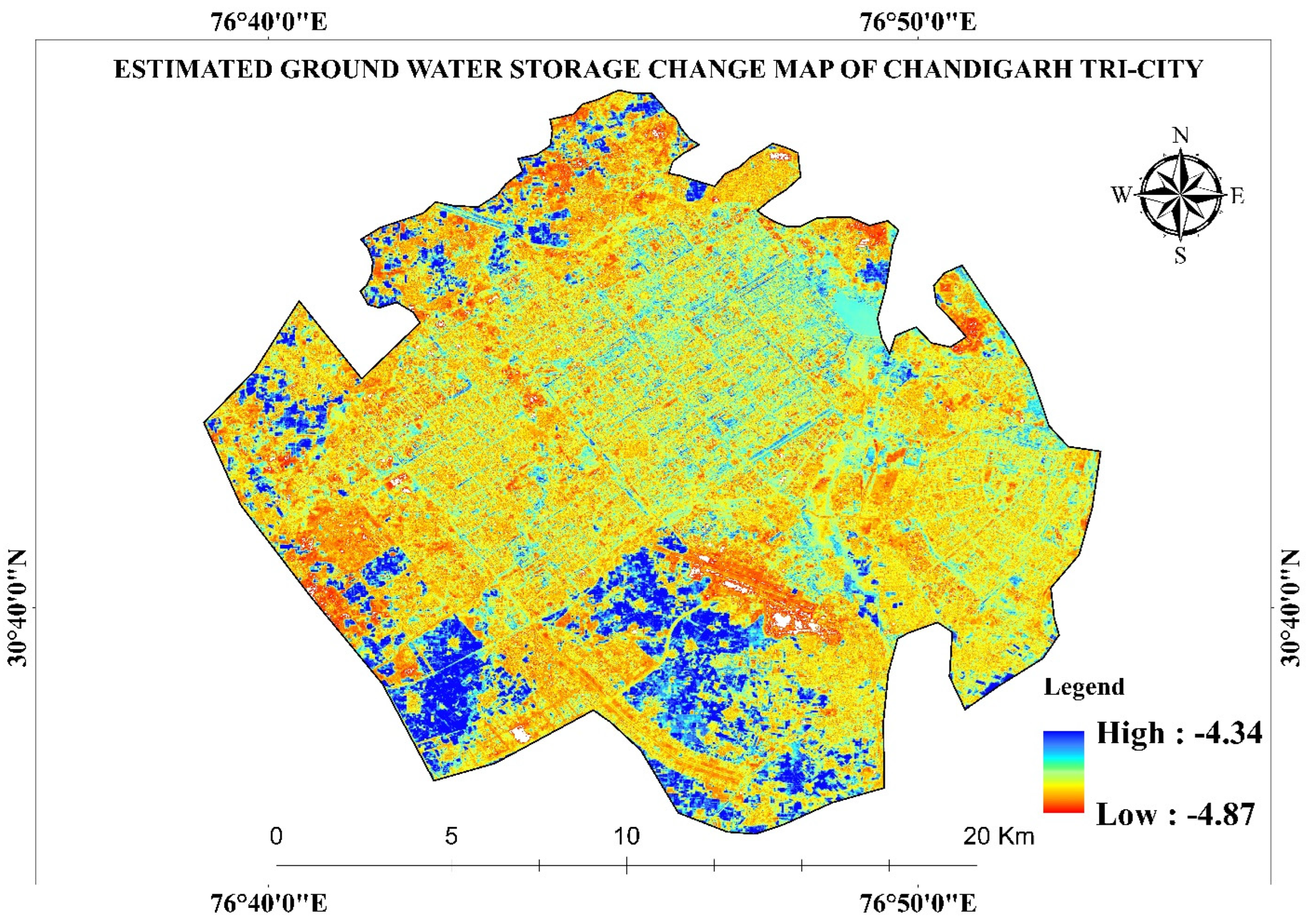
- The estimated average ΔGWS is observed to be −4.605, and the average from GRACE and GLDAS LSM is observed to be −4.587, which is comparable.
5.1. Limitations of the Present Study
5.2. Future Work
Author Contributions
Funding
Data Availability Statement
Acknowledgments
Conflicts of Interest
References
- Elmes, A.; Alemohammad, H.; Avery, R.; Caylor, K.; Eastman, J.R.; Fishgold, L.; Friedl, M.A.; Jain, M. Accounting for Training Data Error in Machine Learning Applied to Earth Observations. Remote Sens. 2020, 12, 1034. [Google Scholar] [CrossRef] [Green Version]
- Choudhury, P.; Gahalaut, K.; Dumka, R.; Gahalaut, V.K.; Singh, A.K.; Kumar, S. GPS measurement of land subsidence in Gandhinagar, Gujarat (Western India), due to groundwater depletion. Environ. Earth Sci. 2018, 77, 770. [Google Scholar] [CrossRef]
- Kayhomayoon, Z.; Arya, N.A.; Milan, S.G.; Moghaddam, K.H.; Berndtsson, R. Novel approach for predicting groundwater storage loss using machine learning. J. Environ. Manag. 2021, 296, 113237. [Google Scholar] [CrossRef]
- Bai, X.; Surveyer, A.; Elmqvist, T.; Gatzweiler, F.W.; Güneralp, B.; Parnell, S.; Prieur-Richard, A.-H.; Shrivastava, P.; Siri, J.G.; Stafford-Smith, M.; et al. Defining and advancing a systems approach for sustainable cities. Curr. Opin. Environ. Sustain. 2016, 23, 69–78. [Google Scholar] [CrossRef]
- Mohamed, M.A.; Anders, J.; Schneider, C. Monitoring of Changes in Land Use/Land Cover in Syria from 2010 to 2018 Using Multitemporal Landsat Imagery and GIS. Land 2020, 9, 226. [Google Scholar] [CrossRef]
- Carrillo-Rivera, J.J.; Cardona, A.; Huizar-Alvarez, R.; Graniel, E. Response of the interaction between groundwater and other components of the environment in Mexico. Environ. Geol. 2008, 55, 303–319. [Google Scholar] [CrossRef]
- Squeo, F.A.; Aravena, R.; Aguirre, E.; Pollastri, A.; Jorquera, C.B.; Ehleringer, J.R. Groundwater dynamics in a coastal aquifer in north-central Chile: Implications for groundwater recharge in an arid ecosystem. J. Arid. Environ. 2006, 67, 240–254. [Google Scholar] [CrossRef]
- Mundepi, A.K.; Lindholm, C.; Kamal. Soft soil mapping using Horizontal to Vertical Spectral Ratio (HVSR) for seismic hazard assessment of Chandigarh city in Himalayan foothills, north India. J. Geol. Soc. India 2009, 74, 551. [Google Scholar] [CrossRef]
- Du, Z.; Ge, L.; Li, X.; Ng, A.H.M. Subsidence Monitoring over the Southern Coalfield, Australia Using both L-Band and C-Band SAR Time Series Analysis. Remote Sens. 2016, 8, 543. [Google Scholar] [CrossRef] [Green Version]
- Milczarek, W. Application of a small baseline subset time series method with atmospheric correction in monitoring results of mining activity on ground surface and in detecting induced seismic events. Remote Sens. 2019, 11, 1008. [Google Scholar] [CrossRef] [Green Version]
- Levien, M. Special economic zones and accumulation by dispossession in India. J. Agrar. Chang. 2011, 11, 454–483. [Google Scholar] [CrossRef]
- Hssaisoune, M.; Bouchaou, L.; Sifeddine, A.; Bouimetarhan, I.; Chehbouni, A. Moroccan groundwater resources and evolution with global climate changes. Geosciences 2020, 10, 81. [Google Scholar] [CrossRef] [Green Version]
- Perrin, J.; Mascré, C.; Pauwels, H.; Ahmed, S. Solute recycling: An emerging threat to groundwater quality in southern India? J. Hydrol. 2011, 398, 144–154. [Google Scholar] [CrossRef]
- Steinhardt, R.; Trafford, B.D. SOME EFFECTS SUB-SURFACE DRAINAGE AND PLOUGHING ON THE STRUCTURE and COMPACTABILITY A CLAY SOIL. J. Soil Sci. 1974, 25, 138–152. [Google Scholar] [CrossRef]
- Arthurton, R.S. Marine-related physical natural hazards affecting coastal megacities of the Asia–Pacific region–awareness and mitigation. Ocean. Coast. Manag. 1998, 40, 65–85. [Google Scholar] [CrossRef]
- Roccheggiani, M.; Piacentini, D.; Tirincanti, E.; Perissin, D.; Menichetti, M. Detection and monitoring of tunneling induced ground movements using Sentinel-1 SAR Interferometry. Remote Sens. 2019, 11, 639. [Google Scholar] [CrossRef] [Green Version]
- Tomás, R.; Romero, R.; Mulas, J.; Marturià, J.J.; Mallorquí, J.J.; López-Sánchez, J.M.; Gutiérrez, F.; González, P.J.; Fernández, J.; Duque, S.; et al. Radar interferometry techniques for the study of ground subsidence phenomena: A review of practical issues through cases in Spain. Environ. Earth Sci. 2014, 71, 163–181. [Google Scholar] [CrossRef] [Green Version]
- Strozzi, T.; Wegmuller, U.; Werner, C.L.; Wiesmann, A.; Spreckels, V. JERS SAR interferometry for land subsidence monitoring. IEEE Trans. Geosci. Remote Sens. 2003, 41, 1702–1708. [Google Scholar] [CrossRef]
- Dehghani, M.; Zoej, M.J.V.; Hooper, A.; Hanssen, R.F.; Entezam, I.; Saatchi, S. Hybrid conventional and persistent scatterer SAR interferometry for land subsidence monitoring in the Tehran Basin, Iran. ISPRS J. Photogramm. Remote Sens. 2013, 79, 157–170. [Google Scholar] [CrossRef]
- Azarakhsh, Z.; Azadbakht, M.; Matkan, A. Estimation, modeling, and prediction of land subsidence using Sentinel-1 time series in Tehran-Shahriar plain: A machine learning-based investigation. Remote Sens. Appl. Soc. Environ. 2022, 25, 100691. [Google Scholar] [CrossRef]
- El Kamali, M.; Abuelgasim, A.; Papoutsis, I.; Loupasakis, C.; Kontoes, C. A reasoned bibliography on SAR interferometry applications and outlook on big interferometric data processing. Remote Sens. Appl. Soc. Environ. 2020, 19, 100358. [Google Scholar] [CrossRef]
- Cavur, M.; Moraga, J.; Duzgun, H.S.; Soydan, H.; Jin, G. Displacement analysis of geothermal field based on PSInSAR and SOM clustering algorithms a case study of Brady Field, Nevada—USA. Remote Sens. 2021, 13, 349. [Google Scholar] [CrossRef]
- Zhang, Y.; Zhang, J.; Wu, H.; Lu, Z.; Guangtong, S. Monitoring of urban subsidence with SAR interferometric point target analysis: A case study in Suzhou, China. Int. J. Appl. Earth Obs. Geoinf. 2011, 13, 812–818. [Google Scholar] [CrossRef]
- Ng, A.H.M.; Ge, L.; Du, Z.; Wang, S.; Ma, C. Satellite radar interferometry for monitoring subsidence induced by longwall mining activity using Radarsat-2, Sentinel-1 and ALOS-2 data. Int. J. Appl. Earth Obs. Geoinf. 2017, 61, 92–103. [Google Scholar] [CrossRef]
- Liosis, N.; Marpu, P.R.; Pavlopoulos, K.; Ouarda, T.B. Ground subsidence monitoring with SAR interferometry techniques in the rural area of Al Wagan, UAE. Remote Sens. Environ. 2018, 216, 276–288. [Google Scholar] [CrossRef]
- Chen, B.; Gong, H.; Lei, K.; Li, J.; Zhou, C.; Gao, M.; Guan, H.; Lv, W. Land subsidence lagging quantification in the main exploration aquifer layers in Beijing plain, China. Int. J. Appl. Earth Obs. Geoinf. 2019, 75, 54–67. [Google Scholar] [CrossRef]
- Tiwari, A.; Narayan, A.B.; Dwivedi, R.; Dikshit, O.; Nagarajan, B. Monitoring of landslide activity at the Sirobagarh landslide, Uttarakhand, India, using LiDAR, SAR interferometry and geodetic surveys. Geocarto Int. 2020, 35, 535–558. [Google Scholar] [CrossRef]
- Govil, H.; Chatterjee, R.S.; Bhaumik, P.; Vishwakarma, N. Deformation monitoring of Surakachhar underground coal mines of Korba, India using SAR interferometry. Adv. Space Res. 2022, 70, 3905–3916. [Google Scholar] [CrossRef]
- Awasthi, S.; Jain, K.; Bhattacharjee, S.; Gupta, V.; Varade, D.; Singh, H.; Narayan, A.B.; Budillon, A. Analyzing urbanization induced groundwater stress and land deformation using time-series Sentinel-1 datasets applying PSInSAR approach. Sci. Total Environ. 2022, 844, 157103. [Google Scholar] [CrossRef]
- Cigna, F.; Bateson, L.B.; Jordan, C.J.; Dashwood, C. Simulating SAR geometric distortions and predicting Persistent Scatterer densities for ERS-1/2 and ENVISAT C-band SAR and InSAR applications: Nationwide feasibility assessment to monitor the landmass of Great Britain with SAR imagery. Remote Sens. Environ. 2014, 152, 441–466. [Google Scholar] [CrossRef] [Green Version]
- Kalsi, N.; Kiran, R. Greater Mohali Region: Geopolitical Impact on Urban Anthropology to Emerge as a Significant Tri-city Entity. J. Hum. Ecol. 2014, 47, 125–137. [Google Scholar] [CrossRef]
- Siddiqui, A.; Kakkar, K.K.; Halder, S.; Kumar, P. Smart Chandigarh Tri-City Region: Spatial Strategies of Transformation. In Smart Metropolitan Regional Development: Economic and Spatial Design Strategies; Kumar, T.M.V., Ed.; Springer: Singapore, 2019; pp. 403–450. [Google Scholar] [CrossRef]
- Jain, S.K.; Agarwal, P.K.; Singh, V.P. Groundwater. In Hydrology and Water Resources of India; Jain, S.K., Agarwal, P.K., Singh, V.P., Eds.; Springer: Dordrecht, The Netherlands, 2007; pp. 235–294. [Google Scholar] [CrossRef]
- Keesari, T.; Sinha, U.K.; Saha, D.; Dwivedi, S.N.; Shukla, R.R.; Mohokar, H.; Roy, A. Isotope and hydrochemical systematics of groundwater from a multi-tiered aquifer in the central parts of Indo-Gangetic Plains, India–implications for groundwater sustainability and security. Sci. Total Environ. 2021, 789, 147860. [Google Scholar] [CrossRef]
- Korisettar, R. Toward developing a basin model for Paleolithic settlement of the Indian subcontinent: Geodynamics, monsoon dynamics, habitat diversity and dispersal routes. In The Evolution and History of Human Populations in South Asia: Inter-disciplinary Studies in Archaeology, Biological Anthropology, Linguistics and Genetics; Petraglia, M.D., Allchin, B., Eds.; Springer: Dordrecht, The Netherlands, 2007; pp. 69–96. [Google Scholar] [CrossRef]
- Gargani, J.; Abdessadok, S.; Tudryn, A.; Sao, C.C.; Malassé, A.D.; Gaillard, C.; Moigne, M.-A.; Singh, M.; Bhardwaj, V.; Karir, B. Geology and geomorphology of Masol paleonto-archeological site, Late Pliocene, Chandigarh, Siwalik Frontal Range, NW India. Comptes Rendus Palevol 2016, 15, 379–391. [Google Scholar] [CrossRef] [Green Version]
- Kandpal, G.C.; Agarwal, K.K. Assessment of liquefaction potential of the sediments of Chandigarh area. J. Geol. Soc. India 2018, 91, 323–328. [Google Scholar] [CrossRef]
- Kadiyan, N.; Chatterjee, R.S.; Pranjal, P.; Agrawal, P.; Jain, S.K.; Angurala, M.L.; Biyani, A.K.; Sati, M.S.; Kumar, D.; Bhardwaj, A.; et al. Assessment of groundwater depletion–induced land subsidence and characterisation of damaging cracks on houses: A case study in Mohali-Chandigarh area, India. Bull. Eng. Geol. Environ. 2021, 80, 3217–3231. [Google Scholar] [CrossRef]
- Ferretti, A.; Prati, C.; Rocca, F. Permanent scatterers in SAR interferometry. IEEE Trans. Geosci. Remote Sens. 2001, 39, 8–20. [Google Scholar] [CrossRef]
- Sowter, A.; Amat, M.B.C.; Cigna, F.; Marsh, S.; Athab, A.; Alshammari, L. Mexico City land subsidence in 2014–2015 with Sentinel-1 IW TOPS: Results using the Intermittent SBAS (ISBAS) technique. Int. J. Appl. Earth Obs. Geoinf. 2016, 52, 230–242. [Google Scholar] [CrossRef]
- Wegnüller, U.; Werner, C.; Strozzi, T.; Wiesmann, A.; Frey, O.; Santoro, M. Sentinel-1 support in the GAMMA software. Procedia Comput. Sci. 2016, 100, 1305–1312. [Google Scholar] [CrossRef] [Green Version]
- Tripathi, A.; Attri, L.; Tiwari, R.K. Spaceborne C-band SAR remote sensing–based flood mapping and runoff estimation for 2019 flood scenario in Rupnagar, Punjab, India. Environ. Monit. Assess. 2021, 193, 110. [Google Scholar] [CrossRef]
- Upreti, M.; Kumar, D. Investigating capability of open archive multispectral and SAR datasets for Wheat crop monitoring and acreage estimation studies. Earth Sci. Inform. 2021, 14, 2017–2035. [Google Scholar] [CrossRef]
- Tripathi, A.; Tiwari, R.K. Synergetic utilization of sentinel-1 SAR and sentinel-2 optical remote sensing data for surface soil moisture estimation for Rupnagar, Punjab, India. Geocarto Int. 2022, 37, 2215–2236. [Google Scholar] [CrossRef]
- Aziz, M.A.; Moniruzzaman, M.; Tripathi, A.; Hossain, M.I.; Ahmed, S.; Rahaman, K.R.; Rahman, F.; Ahmed, R. Delineating flood zones upon employing synthetic aperture data for the 2020 flood in Bangladesh. Earth Syst. Environ. 2022, 6, 733–743. [Google Scholar] [CrossRef]
- Tripathi, A.; Reshi, A.R.; Moniruzzaman, M.; Rahaman, K.R.; Tiwari, R.K.; Malik, K. Interoperability of-Band Sentinel-1 SAR and GRACE Satellite Sensors on PSInSAR-Based Urban Surface Subsidence Mapping of Varanasi, India. IEEE Sens. J. 2022, 22, 21071–21081. [Google Scholar] [CrossRef]
- Tripathi, A.; Tiwari, R.K. Utilisation of spaceborne C-band dual pol Sentinel-1 SAR data for simplified regression-based soil organic carbon estimation in Rupnagar, Punjab, India. Adv. Space Res. 2022, 69, 1786–1798. [Google Scholar] [CrossRef]
- Tripathi, A.; Maithani, S.; Kumar, S. Minimization of the ambiguity of merging of urban builtup and fallow land features by generating ‘C2’ covariance matrix using spaceborne bistatic dual Pol SAR data. In Proceedings of the 2018 4th International Conference on Recent Advances in Information Technology (RAIT), Dhanbad, India, 15–17 March 2018; pp. 1–4. [Google Scholar] [CrossRef]
- Tripathi, A.; Maithani, S.; Kumar, S. X-band persistent SAR interferometry for surface subsidence detection in Rudrapur City, India. Remote Sens. Technol. Appl. Urban Environ. III SPIE 2018, 10793, 105–115. [Google Scholar] [CrossRef]
- Tripathi, A.; Tiwari, R.K. A simplified subsurface soil salinity estimation using synergy of SENTINEL-1 SAR and SENTINEL-2 multispectral satellite data, for early stages of wheat crop growth in Rupnagar, Punjab, India. Land Degrad. Dev. 2021, 32, 3905–3919. [Google Scholar] [CrossRef]
- Li, Z.; Cao, Y.; Wei, J.; Duan, M.; Wu, L.; Hou, J.; Zhu, J. Time-series InSAR ground deformation monitoring: Atmospheric delay modeling and estimating. Earth-Sci. Rev. 2019, 192, 258–284. [Google Scholar] [CrossRef]
- Talib, O.C.; Shimon, W.; Sarah, K.; Tonian, R. Detection of sinkhole activity in West-Central Florida using InSAR time series observations. Remote Sens. Environ. 2022, 269, 112793. [Google Scholar] [CrossRef]
- Chen, J. Satellite gravimetry and mass transport in the earth system. Geod. Geodyn. 2019, 10, 402–415. [Google Scholar] [CrossRef]
- Ramillien, G.; Frappart, F.; Seoane, L. Application of the regional water mass variations from GRACE satellite gravimetry to large-scale water management in Africa. Remote Sens. 2014, 6, 7379–7405. [Google Scholar] [CrossRef] [Green Version]
- Zencich, S.J.; Froend, R.H.; Turner, J.V.; Gailitis, V. Influence of groundwater depth on the seasonal sources of water accessed by Banksia tree species on a shallow, sandy coastal aquifer. Oecologia 2001, 131, 8–19. [Google Scholar] [CrossRef]
- Singh, A.; Seitz, F.; Schwatke, C. Inter-annual water storage changes in the Aral Sea from multi-mission satellite altimetry, optical remote sensing, and GRACE satellite gravimetry. Remote Sens. Environ. 2012, 123, 187–195. [Google Scholar] [CrossRef]
- Vishwakarma, B.D.; Zhang, J.; Sneeuw, N. Downscaling GRACE total water storage change using partial least squares regression. Sci. Data 2021, 8, 95. [Google Scholar] [CrossRef]
- Castellazzi, P.; Martel, R.; Galloway, D.L.; Longuevergne, L.; Rivera, A. Assessing groundwater depletion and dynamics using GRACE and InSAR: Potential and limitations. Groundwater 2016, 54, 768–780. [Google Scholar] [CrossRef] [PubMed] [Green Version]
- Agarwal, V.; Kumar, A.; Gomes, R.L.; Marsh, S. Monitoring of ground movement and groundwater changes in London using InSAR and GRACE. Appl. Sci. 2020, 10, 8599. [Google Scholar] [CrossRef]
- Eckle, K.; Schmidt-Hieber, J. A comparison of deep networks with ReLU activation function and linear spline-type methods. Neural Netw. 2019, 110, 232–242. [Google Scholar] [CrossRef]
- Kurtenbach, E.; Mayer-Gürr, T.; Eicker, A. Deriving daily snapshots of the Earth’s gravity field from GRACE L1B data using Kalman filtering. Geophys. Res. Lett. 2009, 36, 1–5. [Google Scholar] [CrossRef]
- Güntner, A. Improvement of global hydrological models using GRACE data. Surv. Geophys. 2008, 29, 375–397. [Google Scholar] [CrossRef] [Green Version]


| SL.No. | Datasets | Polarization | Period |
|---|---|---|---|
| 1. | Sentinel-1 SAR Single Look Complex (SLC) data | VV+VH Ascending (26 images) and Descending pass (26 images) | 2017–2022 |
| 2. | Groundwater level data from CGWB | -------- | 2017–2022 |
| 3. | GRACE monthly terrestrial water storage data | -------- | 2017–2022 |
| 4. | GLDAS LSM soil moisture and surface water | -------- | 2017–2022 |
| S.No. | Area/Location of Well/Domestic Boring | PSInSAR-Based Surface Displacement (in mm) 2017–2022 | Reported Groundwater Level (mbgl) in 2017 from Field Data Collection | Reported Groundwater Level in 2022 from Field Data Collection |
|---|---|---|---|---|
| 1. | Sector-43 | −40 | 40 | 41 |
| 2. | Airport area | −37 | 20 | 22 |
| 3. | Sector-12 PEC Campus | −33 | 25 | 27 |
| 4. | Sector-17 | 30 | 37 | 38 |
| 5. | Sector- 33 | 25 | 36 | 39 |
| 6. | Sector-29 | −28 | 15 | 16 |
| 7. | Sector-39 | −24 | 12 | 15 |
| 8. | Sector-20 | −22 | 10 | 14 |
| 9. | Sector-7 | −35 | 5 | 7 |
| 10. | Sector-47 | −31 | 21 | 22 |
Disclaimer/Publisher’s Note: The statements, opinions and data contained in all publications are solely those of the individual author(s) and contributor(s) and not of MDPI and/or the editor(s). MDPI and/or the editor(s) disclaim responsibility for any injury to people or property resulting from any ideas, methods, instructions or products referred to in the content. |
© 2023 by the authors. Licensee MDPI, Basel, Switzerland. This article is an open access article distributed under the terms and conditions of the Creative Commons Attribution (CC BY) license (https://creativecommons.org/licenses/by/4.0/).
Share and Cite
Reshi, A.R.; Sandhu, H.A.S.; Cherubini, C.; Tripathi, A. Estimating Land Subsidence and Gravimetric Anomaly Induced by Aquifer Overexploitation in the Chandigarh Tri-City Region, India by Coupling Remote Sensing with a Deep Learning Neural Network Model. Water 2023, 15, 1206. https://doi.org/10.3390/w15061206
Reshi AR, Sandhu HAS, Cherubini C, Tripathi A. Estimating Land Subsidence and Gravimetric Anomaly Induced by Aquifer Overexploitation in the Chandigarh Tri-City Region, India by Coupling Remote Sensing with a Deep Learning Neural Network Model. Water. 2023; 15(6):1206. https://doi.org/10.3390/w15061206
Chicago/Turabian StyleReshi, Arjuman Rafiq, Har Amrit Singh Sandhu, Claudia Cherubini, and Akshar Tripathi. 2023. "Estimating Land Subsidence and Gravimetric Anomaly Induced by Aquifer Overexploitation in the Chandigarh Tri-City Region, India by Coupling Remote Sensing with a Deep Learning Neural Network Model" Water 15, no. 6: 1206. https://doi.org/10.3390/w15061206