Use of Soil Infiltration Capacity and Stream Flow Velocity to Estimate Physical Flood Vulnerability under Land-Use Change Scenarios

Abstract

Land-use changes produce variations in upper soil hydraulic properties and alter the hydrological response and hydraulic behavior of streams. Thus, the combined effect of variations in soil properties and current hydraulics interacts with the exposure of structures exposed and their degree of physical vulnerability. This study aims to evaluate the effect of land-use evolution from 1976 to 2017 on the physical vulnerability of structures exposed to floods in the Combeima cathment, Colombia, proposing two novel approaches: (i) based on soil infiltration capacity variation (CN) in the basin and changes in stream flow velocity (v), (ii) through soil water storage variation in the root zone (Hu). Hydrological and hydraulic modeling and the implementation of four physical vulnerability assessment methods were performed using GIS analysis. Findings indicate that simplifying physical vulnerability estimations through CN, Hu, and $v$ variations in catchments and at cross-section resolutions is possible, allowing a detailed analysis of the land-use change effect on the vulnerability of structures. The scaling behavior of the physical vulnerability of structures was identified when Hu is defined as a scale variable and, similarly, concerning flow velocity in the stream. Therefore, applying the power law could be useful in planning processes with limited information.

1. Introduction

Catastrophic events and physical damage due to natural processes are increasing worldwide [1], mainly affecting developing countries [2]. Floods are one of many recurrent hydrometeorological events and produce the most significant losses [3]. In this sense, flood risk management must incorporate elements associated with understanding the threats and their relationship with economic development and land-use and climate changes [4], among others, which affect the magnitude of floods [5] and the physical vulnerability of structures exposed to them. Once integrated and understood, adequate mitigation and adaptation measures can be designed [6].

The term vulnerability has been defined as the probability of an element being affected by the occurrence of a threatening event [7]. In this sense, the physical dimension of vulnerability encompasses the susceptibility of structures that can be negatively affected by a threatening event [8]. Various methods have been proposed to assess vulnerability conceptualizing the relationship between the magnitude of the flood event and its effect on the exposed element [9]. Currently, the concept of vulnerability considers variables such as the effect of an event on spatial, temporal, and social factors [10], resistance, resilience, and susceptibility [11], the degree of exposure, protection, recovery, and reconstruction [12], and the degree of structural and non-structural damage relative to the intensity of the threat [13,14]. In practical terms, to assess vulnerability, various techniques have been used, such as the simulation of the degree of damage or failure of structures [15], the empirical evaluation carried out after the occurrence of the event [16], the elaboration of damage curves [17], and the estimation of the magnitude of floods [18], among others. Furthermore, some researchers have suggested that vulnerability should be analyzed as a dynamic characteristic resulting from the interactions between individual, social, structural, and dimensional factors, which can vary temporarily or change over time [19,20].

Conversely, climate and land-use changes, among others, have been recognized to affect the hydrological response of basins in the flood regime [21,22]. In the specific case of evaluating the physical vulnerability of structures exposed to floods in a land-use change scenario, some methods such as those based on visible damage rating [23], land-use patterns measurement and mapping [24], the concept of Emergy to perform an economic analysis of flood occurrence [25], morphological variables and soil characteristics in basins [26], among others have been proposed. However, such analyses require the use of large data sets that, in some cases, may not be available, making implementation challenging.

Based on the above, this research proposes to evaluate the physical vulnerability to flooding using a method that incorporates variables related to soil infiltration capacity dynamics in the basin as an effect of the vegetation cover change and the hydrological response of the basin on the hydraulic behavior of the stream in a cross-section with an exposed structure. Accordingly, the aims of this study are (i) to evaluate the physical vulnerability of structures to floods in a land-use change scenario; (ii) to propose the evaluation of the physical vulnerability of structures through the variation of the infiltration capacity represented by the curve number (CN) proposed by [27], soil water storage in the root zone (Hu), and stream flow velocity (v) in a cross-section with an exposed structure, and (iii) to examine the scaling properties of physical vulnerability in relation to CN, Hu, and $v$. For this, the hydrological and hydraulic modeling of the Combeima river catchment located in Colombia will be carried out to evaluate the land-use change effect during the 1976–2017 period in 22 structures, such as bridges and retaining walls located along the main stream.

2. Materials and Methods

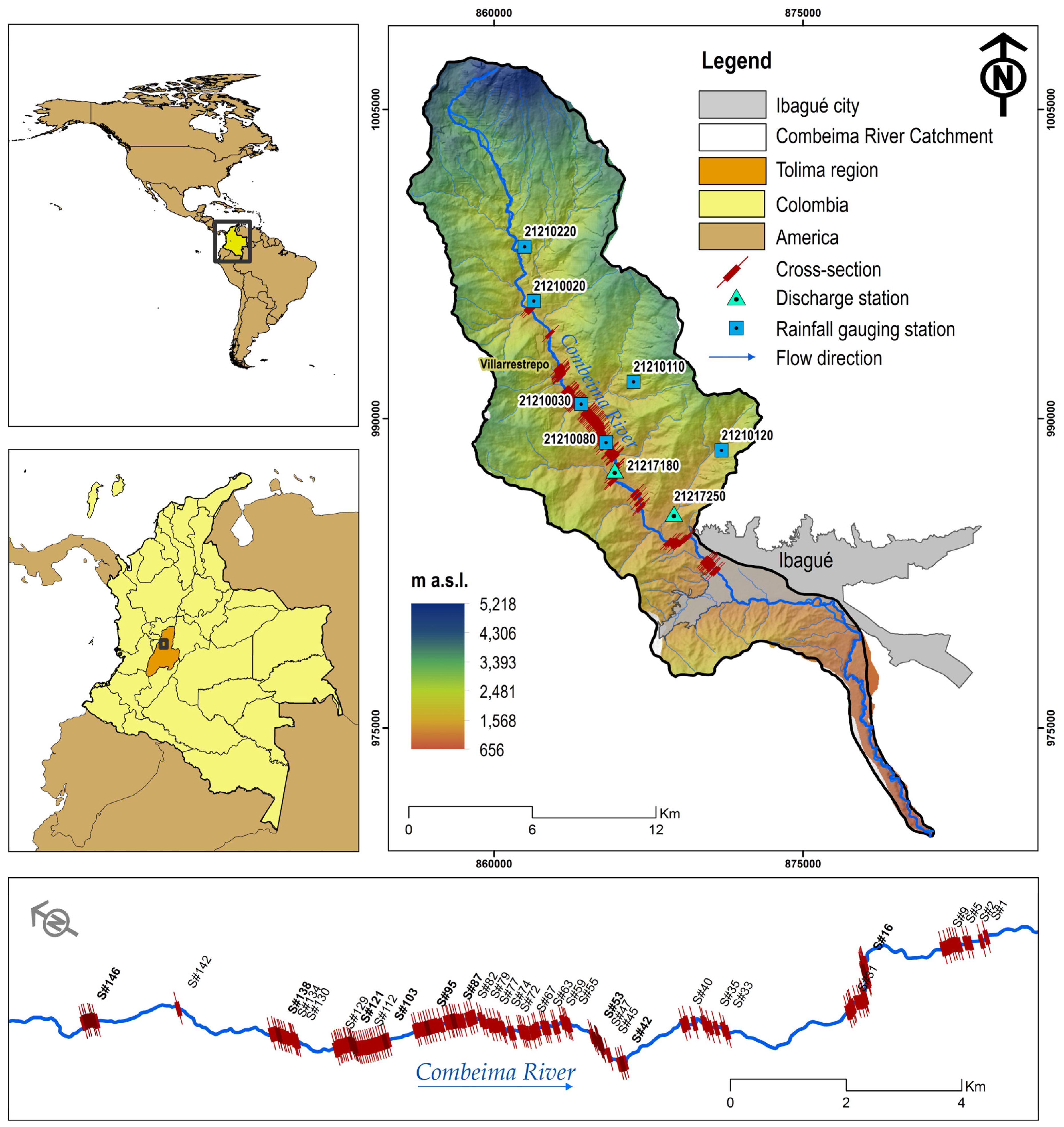
2.1. Study Area

The hydrological and hydraulic modeling of the Combeima river catchment, located in the intertropical convergence zone in Colombia, was carried out (Figure 1). The basin has a drainage area of 274 km² and an elevation range between 5150 and 700 m a.s.l. It has a bimodal rainfall regime with an annual average of 1816 mm and an average temperature of 16 °C. The main stream is predominantly mountainous with a length of 57.4 km, an average slope of 8.47%, and an average and maximum annual flow of 4893 and 8828 m³ s⁻¹, respectively. At elevations above 4000 m a.s.l., there is paramo vegetation, and in the rest of the basin, there are evergreen forests, subsistence crops, and grassland areas with scattered bushes.

Geologically, the basin is mainly comprised of metamorphic rocks belonging to the lithostratigraphic units Gneiss and Amphibolites of Tierradentro (gneisses, amphibolites, and mylonites), Metasedimentites of Santa Teresa (cherts, subgrawacas, and lidites) and the Cajamarca Complex (black and green schists, amphibolites, marbles, serpentinites, and mylonites).

The hydraulic property values of the soil in the Combeima river basin reported by [28] and obtained applying the pedotransfer functions proposed by [29] were employed in this study. Hence, soil water storage in the root zone (Hu) and vertical (Ks) and horizontal (Kss) hydraulic conductivity values were weighted according to the depth of each soil horizon for hydrological modeling and correspond to modal values (

Table 1. Modal values of the hydraulic properties of soils in the Combeima river basin, Colombia, reported by Peña et al. (2016) [28]. * Taxonomic classification of soils defined by the United States Department of Agriculture (USDA) [30,31].

Soil Unit *	Forest			Grassland			Crop
	$\mathit{H}\mathit{u}$ (mm)	$\mathit{K}\mathit{s}\mathit{s}$ (mm h−1)	$\mathit{K}\mathit{s}$ (mm h−1)	$\mathit{H}\mathit{u}$ (mm)	$\mathit{K}\mathit{s}\mathit{s}$ (mm h−1)	$\mathit{K}\mathit{s}$ (mm h−1)	$\mathit{H}\mathit{u}$ (mm)	$\mathit{K}\mathit{s}\mathit{s}$ (mm h−1)	$\mathit{K}\mathit{s}$ (mm h−1)
MKB	102.6	75.7	68.2	10.3	7.6	6.8	24.6	18.2	16.4
MKG	153.2	58.2	57.9	22.8	8.8	8.7	54.6	21.0	20.8
MQC	149.3	28.0	28.6	11.6	2.0	2.0	27.9	4.8	4.8
MQD	140.1	177.7	114.7	11.9	14.5	9.4	28.6	34.9	22.5
MQE	194.9	22.8	22.2	18.0	2.1	2.1	43.3	5.1	4.9
MDA	100.8	105.8	80.9	8.5	8.9	6.8	20.4	21.4	16.3
MGA	54.9	236.7	114.5	54.9	236.7	114.5	54.9	236.7	114.5
MGB	133.3	576.5	104.6	4.5	21.5	10.5	10.9	51.5	25.2
MGC	93.2	119.4	78.0	23.0	99.4	18.0	55.2	238.6	43.3
MWD	0.0	3011.7	3008.6	0.0	3011.7	3008.6	0.0	3011.7	3008.6
PWD	117.7	14.9	14.1	9.0	1.1	1.0	21.6	2.7	2.5
PWL	112.6	203.0	53.6	5.6	10.6	2.7	13.5	24.4	6.4
MQO	126.5	29.7	20.9	19.8	4.6	3.3	47.4	11.1	7.8
MKI	40.4	454.4	127.4	3.2	36.1	10.1	7.7	86.5	24.3
MQH	130.8	12.4	11.6	21.4	2.0	1.9	51.3	4.9	4.6
MQJ	129.6	9.9	7.9	13.9	1.1	851.6	33.4	2.5	2.0
MWA	0.0	10.6	10.0	0.0	1.9	1.8	0.0	4.5	4.3
MWC	0.0	14.4	13.9	0.0	2.9	2.8	0.0	6.9	6.6
MWJ	123.1	20.1	12.1	14.3	2.3	1.4	34.3	5.6	3.4
PWH	50.5	186.9	155.6	3.4	12.6	10.5	8.2	30.3	25.2

).

2.2. Hydrologic and Hydraulic Modeling

The TETIS hydrological model v9.1 [32] was implemented for its ability to represent the rainfall-runoff process in a land-use change scenario [31,32,33,34]. The modeling was carried out with a cell size of 90 m × 90 m, based on vegetation cover maps of the study area elaborated by Instituto Geográfico Agustín Codazzi and Corporación Autónoma Regional del Tolima at a scale of 1:25,000 in the years 1976, 1981, 1991, 2000, 2007, and 2017. Likewise, the time series of seven precipitation stations with daily temporal resolution were employed (Figure 1). This allowed analyzing 41 years of land-use changes in ten-year periods. Thus, it is possible to detect changes in runoff when analyzing land-use changes in 11-year intervals on a daily scale. In this case, the temporal resolution and the analysis period are consistent with various studies [35,36]. Likewise, the 2017–2018 period was used for calibration, and the one from 1984 to 1985 was utilized for validation. The Nash–Sutcliffe Efficiency (NSE) index was used to assess the predictive skill of the hydrological model.

Flow behavior in the Combeima river course was modeled with the one-dimensional HEC-RAS v5.0.7 model of the Army Corps of Engineers, extensively applied in present-day modeling (e.g., [37]). A 20 km long section of the river was analyzed between the town of Villa-Restrepo and the city of Ibagué (Figure 1). One hundred and forty-eight cross-sections of the stream were measured. Twenty-four of these were associated with infrastructure subject to being evaluated for their physical vulnerability to floods in land-use change scenarios (Figure 1), including two catchment structures, nine retaining walls, and 13 bridges.

In this analysis, three types of boundary conditions were defined: (i) the geometry of the cross-sections of the stream, (ii) the roughness parameter to the right, center, and left of the channel of each cross-section, and (iii) the flows and water depth measured at the upstream and downstream border of the study reach. The cross-section width was variable, ranging from 40 to 60 m, and Manning’s roughness coefficients (n) were defined as varying between 0.03 and 0.04 in the center of the channel and between 0.04 and 0.06 on the left and right stream banks. Steady flow calibration was performed by adjusting Manning’s roughness parameter until differences of less than 20% were obtained between the observed and simulated water depth in each cross-section [38].

2.3. Physical Vulnerability Assessment

Two new methods were proposed to estimate the physical vulnerability of structures exposed to floods in land-use change scenarios at the basin scale: (i) vulnerability based on flow velocity and curve number (VFVCN) and (ii) vulnerability based on soil water storage variation (VVHu). These were then contrasted with state-of-the-art methods such as the vulnerability and mapping of floods based on land-use patterns (MFLUP) [39] and the vulnerability in land-use change scenarios (VLUCS) [26], allowing the quantification of the similarity between the evaluated methods.

2.3.1. Vulnerability Based on Flow Velocity and Curve Number (VFVCN)

In this method, the physical vulnerability ($V_{ij}$) of structure $i$ in cross-section $j$ is evaluated as a function of the flow velocity ($v_{ij}$) in cross-section $j$ where structure i is located, and $C{N}_{jk}$ is the infiltration capacity of area $k$ of the catchment basin in cross-section $j$, corresponding to the curve number proposed by USDA-SCS (1972) and represented as shown in Equation (1).

𝑉_𝑖𝑗 = 𝑣_𝑖𝑗 ∩ 𝐶𝑁_𝑗𝑘

(1)

2.3.2. Vulnerability Based on Soil Water Storage Variation (VVHu)

In this model, $V_{ij}$ is evaluated as a function of the flow velocity ($v_{ij}$) and the soil water storage variation in the root zone in afferent area $k$ of cross-section $j$ where the exposed structure ($H{u}_{jk}$) is exposed. This can be expressed as indicated in Equation (2).

$$V_{ij}=v_{ij}{\displaystyle \cap }H{u}_{jk}$$

(2)

2.3.3. Vulnerability and Mapping of Floods Based on Land-Use Patterns (MFLUP)

The vulnerability assessment proposed by [24] was carried out using the MFLUP method for urban areas as a function of the inverse of distance d of structure $i$ to the center of the flood zone in cross-section $j$ and the quotient between the number of affected structures and the total number of structures exposed to a flood event. However, since the analysis performed in this study was not carried out in an urban environment, the method was adapted as described in Equation (3).

$$V_{ij}=\frac{1}{d_{ij}} {\displaystyle \cap } \frac{h_{ij}}{H_{ij}}$$

(3)

where, $V_{ij}$ is the physical vulnerability of structure $i$ in cross-section $j,$ $d_{ij}$ is the distance of structure $i$ to the center of the floodplain in cross-section $j$, $h_{ij}$ represents the maximum water sheet depth over the exposed structure i in cross-section $j$ during the flood event, and $H_{ij}$ is the height of the exposed structure $i$ in cross-section $j$.

2.3.4. Vulnerability in Land-Use Change Scenarios Based on Morpho-Edaphological Attributes (VLUCS)

As part of the validation process of the VFVCN and VVHu methods, the VLUCS model proposed by [26] for the evaluation of the physical vulnerability ($V_{ij}$) as a function of the weighted combination of morpho-edaphological attributes of the basin was implemented, considering as the closing point section $j$, where structure $i$ is located. In the current study, the evaluation of the physical vulnerability in afferent area $k$ of cross-section $j$, where the exposed structure $i$ is located, was considered as indicated in Equation (4).

$$V_{ij}=a\times S_{tk}+b\times A_i+c\times S_{pk}+d\times L{u}_{jk}$$

(4)

where, $S_{tk}$ is the soil type in the afferent area, $A_i$ is the elevation to which the exposed structure is exposed, and $S_{pk}$ is the slope of afferent area $k$ to cross-section $j$ where the exposed structure $i$ is located. $L{u}_{jk}$ corresponds to the current soil use, and coefficients $a$, $b$, $c$, and $d$ represent the weights of each attribute.

2.3.5. Mapping Physical Vulnerability Levels

The analysis considered the water depth due to its relationship with the physical vulnerability of a structure to floods to define the levels of vulnerability and elaborate the maps that represent it. This approach has widely been used because of its ease in obtaining level measurements in streams [38,39,40].

The physical vulnerability levels per method were defined according to the water depth and relative to the total height of the exposed structure in the cross-section of a stream. These values were obtained from the hydraulic simulation of the stream. When water depth ($h_{ij}$) was <33% of the height of the exposed structure, the vulnerability level was considered low. When 3% of the $h_{ij}$ ≤ 66%, the vulnerability level was medium, and when $h_{ij}$ > 66%, the level was considered high.

2.4. Similarity between Vulnerability Assessment Methods

The similarity between the implemented methods was evaluated by applying hierarchical clustering [41] to validate the results obtained from the physical vulnerability of structures exposed to floods in land-use change scenarios per method. The levels of physical vulnerability defined in the high, medium, and low categories were grouped in an agglomerative hierarchical clustering (AHC) based on a distance matrix to measure the similarity between the applied methods. In this study, the similarity was considered more realistic when its magnitude reached values higher than 0.75 [42]. AHC has extensively been applied in flood risk analysis (e.g., [43]).

2.5. Statistical Scaling of Physical Vulnerability

Changes in land-use have been reported to modify the hydraulic properties of soil and affect the maximum streamflow magnitude [42,43]. Likewise, the wide-sense simple scaling (WSSS) flood regime with upper soil hydraulic properties has been verified at the basin scale [28]. Therefore, this study proposes to examine the WSSS of physical flood vulnerability of structures within a basin under land-cover change scenarios with $Hu$, $CN$, and $v_{ij}$ as scales. To this end, the WSSS was described as $Y_{\mathsf{\lambda }}\stackrel{\scriptscriptstyle\mathrm{def}}{=}{\mathsf{\lambda }}^{\mathsf{\alpha }}{Y}_s$ where ≝ shows equality in the probability distributions of exceedance, λ is the scale factor that, in this case, can be $Hu$, $CN$ or $v_{ij}$, and α is the scale exponent. Under these conditions, physical vulnerability is represented as the observed variable $V_{\mathsf{\lambda }}$ that has finite moments $E\left[V_{\mathsf{\lambda }}^r\right]$ of order r, and the aleatory variables ($V_{\mathsf{\lambda }}^r$) and $\left({\mathsf{\lambda }}^{\mathsf{\alpha }}{V}_s\right)$ have the same probability distribution, indicating the invariance with scale λ. Thus, the scaling exponent is a linear function of r that is related to the WSSS [44] (Equation (5)) and, according to [28], it can be expressed as (i) the linearity of the logarithm of moments m of order r, expressed as $log{m}_r\left(\mathsf{\lambda }\right)$ versus $log\mathsf{\lambda }$ for each r, and (ii) by the linearity of the r scale exponents (Equation (5)).

$$\log E\left[V_{\lambda }^r\right]=rn\log \lambda +\log E\left[V_{\lambda }^r\right]$$

(5)

3. Results and Discussion

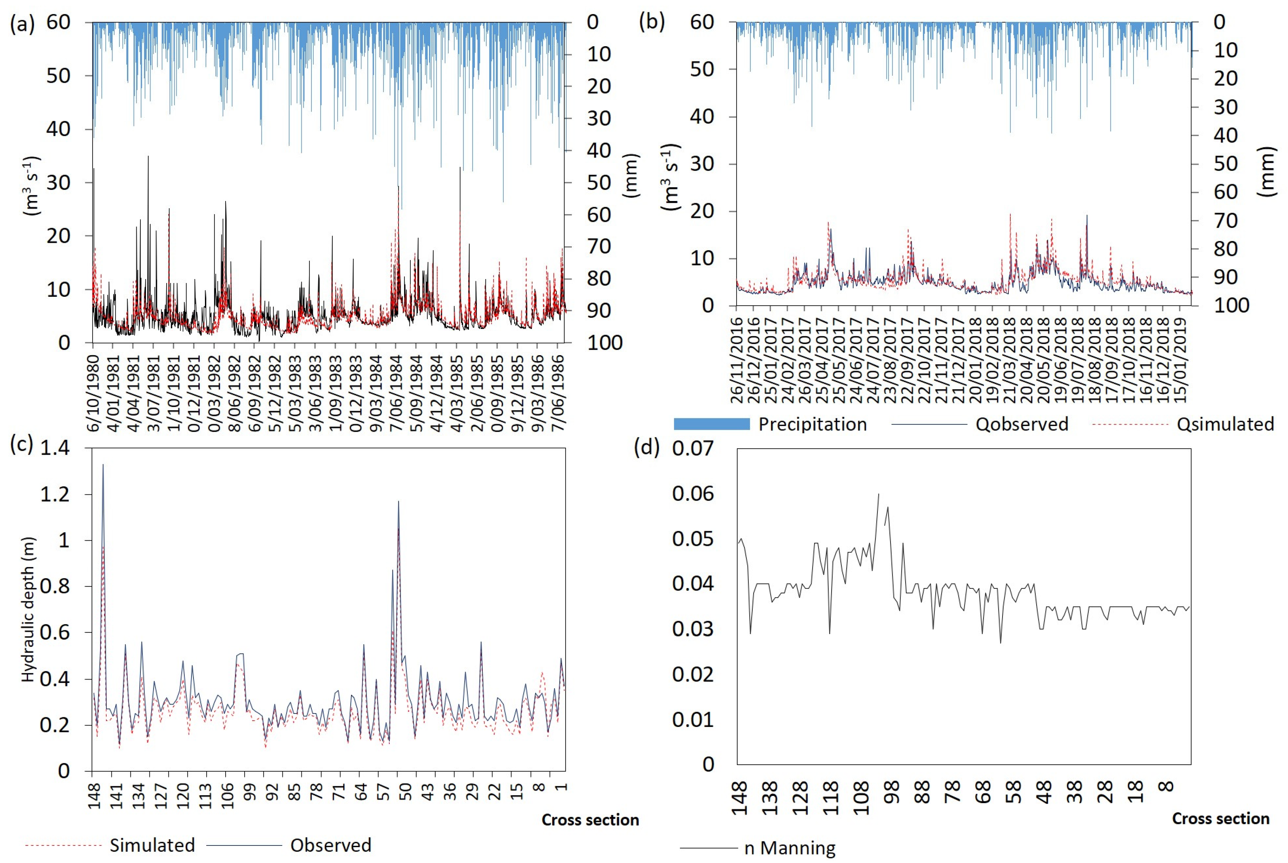
3.1. Calibration and Validation of Models

The Nash–Sutcliffe Efficiency (NSE) index values obtained in the calibration and validation phases were 0.601 for the 1984–1985 period and 0.63 for the 2017–2018 period (Figure 2a,b). These values indicate that the model appropriately describes the rainfall–runoff process [45] and, in this case, those corresponding to the maximum flows in the study area. Otherwise, when calibrating the hydraulic model, differences of less than 12% were found between the observed and calculated depth in 148 cross-sections of the simulated stream reach, leading to using Manning’s n coefficients in a value range between 0.03 and 0.06 (Figure 2c,d).

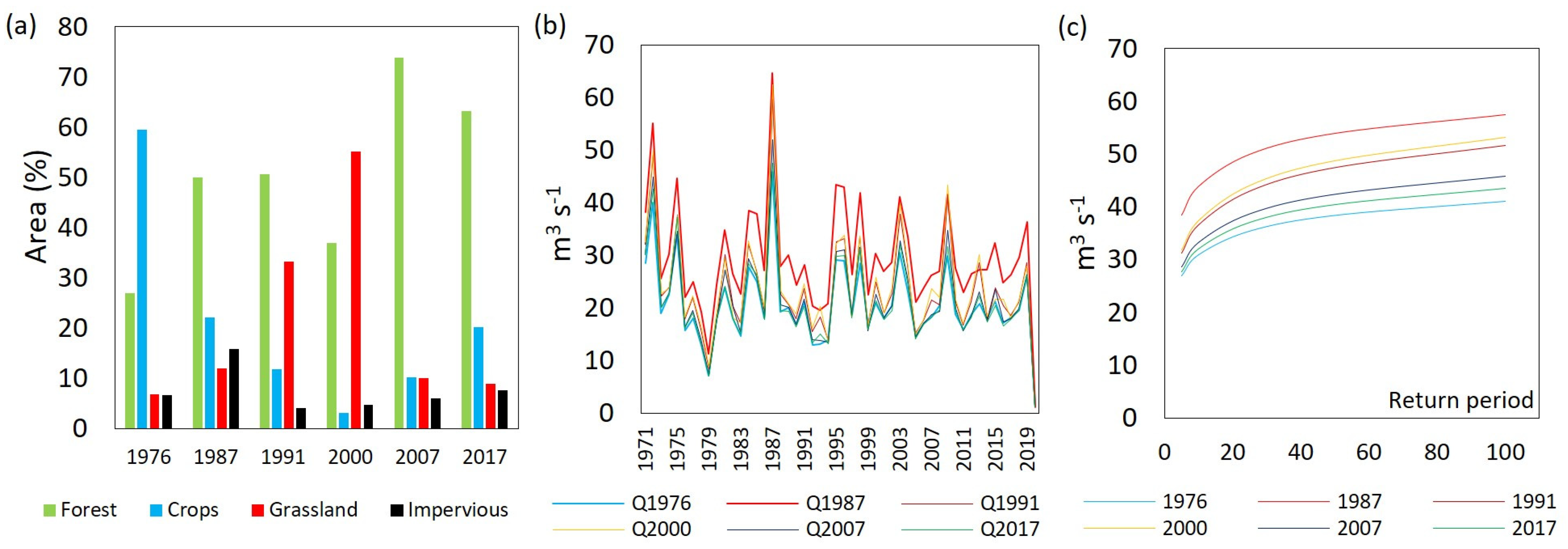
3.2. Effect of Land-Use Change on the Flood Regime

The land-use change effect on the maximum flows at the basin scale can be identified since the size of the basin analyzed corresponds to a mesoscale [22]. In this study, the results of the hydrological modeling indicate that the lowest magnitudes of the maximum flows occurred during the years 1976 and 2017 when the basin covers were predominantly forests and crops. In contrast, between the years 1987 and 2000, the highest magnitudes of the peak flows were registered when grassland areas in the basin predominated (Figure 2). Different researchers [36,46] have reported similar results when evaluating land-use change employing hydrological modeling and are consistent with observations made in experimental plots by [47]. These results are due to soil infiltration capacity variation as a land-use change effect in hydrographic basins [43,46]. Similarly, applying the Generalized Extreme Value (GEV) function for a 100-year return period, the flood frequency analysis for each land-use change scenario showed the largest quantile magnitudes in 1987 and 2000, when grassland areas predominated in the basin (Figure 3).

Figure 3 and

Table 2. Hydraulic characteristics of cross-sections per year.

Year	Cross-Section Number	Velocity (m s−1)	Water Depth (m)	Qmax (m3 s−1)	$\mathit{H}\mathit{u}$ (mm)	$\mathit{K}\mathit{s}$ (mm h−1)	$\mathit{C}\mathit{N}$
1976	53	3.19	1.35	41.12	60.73	15.52	58
	52	1.48	2.94	41.12	82.99	14.34	58
	51	3.49	2.20	41.12	126.50	20.86	58
	49	3.59	1.58	41.12	67.27	24.74	58
	48	4.45	1.33	41.12	37.65	19.10	58
	42	4.76	1.09	41.12	54.05	15.52	58
1987	53	3.57	1.61	57.56	86.68	15.14	59
	52	1.18	3.34	57.56	81.05	14.34	59
	51	3.64	2.62	57.56	126.50	14.34	59
	49	3.99	1.91	57.56	107.73	15.14	59
	48	4.84	1.66	57.56	137.90	11.22	59
	42	5.50	1.24	57.56	80.72	15.52	58
1991	53	3.44	1.52	51.61	74.74	3.57	58
	52	1.69	3.21	51.61	43.29	3.91	58
	51	3.64	2.45	51.61	47.40	3.91	58
	49	3.86	1.79	51.61	40.90	4.20	58
	48	4.75	1.54	51.61	37.65	4.20	58
	42	5.18	1.20	51.61	106.02	3.15	59
2000	53	3.48	1.54	53.18	74.74	12.41	59
	52	1.72	3.24	53.18	43.29	14.34	59
	51	3.64	2.50	53.18	47.40	14.34	59
	49	3.90	1.83	53.18	40.90	11.15	59
	48	4.76	1.56	53.18	37.65	11.15	59
	42	5.27	1.21	53.18	106.02	15.52	60
2007	53	3.30	1.43	45.84	74.74	15.52	48
	52	1.57	3.07	45.84	43.29	7.82	48
	51	3.62	2.30	45.84	47.40	7.82	48
	49	3.73	1.68	45.84	40.90	6.30	48
	48	4.61	1.432	45.84	37.65	6.30	48
	42	4.92	1.146	45.84	106.02	6.30	47
2017	53	3.25	1.39	43.56	74.74	8.36	41
	52	1.53	3.01	43.56	43.29	14.34	41
	51	3.56	2.25	43.56	47.40	14.34	41
	49	3.67	1.63	43.56	40.90	19.10	41
	48	4.56	1.34	43.56	37.65	19.10	41
	42	4.87	1.34	43.56	106.02	15.52	43

indicate that during the 1976–1987 scenarios, the forest, grassland, and impervious surface areas increased by 22.98, 5.22, and 9.25%, respectively, and the crop areas decreased by 37.45%. These changes led to an increase in the maximum flow rate, flow velocity, and depth by 40.00%, 8.82%, and 23.22%, respectively. It is important to clarify that in the current study, populated centers, rocky outcrops, and glaciers were considered impervious surfaces. In the water catchment area assessed, the glacier of the Tolima volcano, located from 4700 up to 5150 m a.s.l., has reduced its size from 1985 to 1991, according to the land-use maps available. Furthermore, during this period, a catastrophic flood event forced the relocation of the town center of Juntas [48]. This event explains, in part, the decrease in the impervious surface between 1987 and 1991 (Figure 3). During the 1987–1991 scenarios, grassland and forests occupied 33.19% and 50.72% of the basin area, producing a decrease in flow velocity, water height, and peak flow by 4.58%, 22.46 %, and 10.34%, respectively.

On the other hand, in the 1991 and 2000 scenarios, areas with forests and crops decreased by 13.75 and 8.70%, while grassland and impervious surfaces increased by 21.96 and 0.49%, respectively. These changes led to an increase in the flow velocity, depth, and maximum discharge of the stream by 2.35, 1.07, and 3.04%, respectively. This behavior is similar to that reported by [42,49] and could be related to the decrease in soil infiltration capacity that produces, in turn, an increase in surface runoff [50].

Similarly, in the 2000 and 2007 scenarios, areas with forests and crops increased by 36.82 and 6.96%, and grassland areas decreased by 45.12%. These changes led to a decrease in the maximum flow rate by 13.79% (Figure 4). Likewise, in 2007 and 2017, the crop area increased by 10.13%, and the grassland area decreased by 1.13%, leading to a reduction in velocity, water height, and maximum flow by 3.80, 11.11, and 4.99%, respectively. These results are consistent with observations reported by [51,52] in experimental plots and by [50,53] in hydrological modeling.

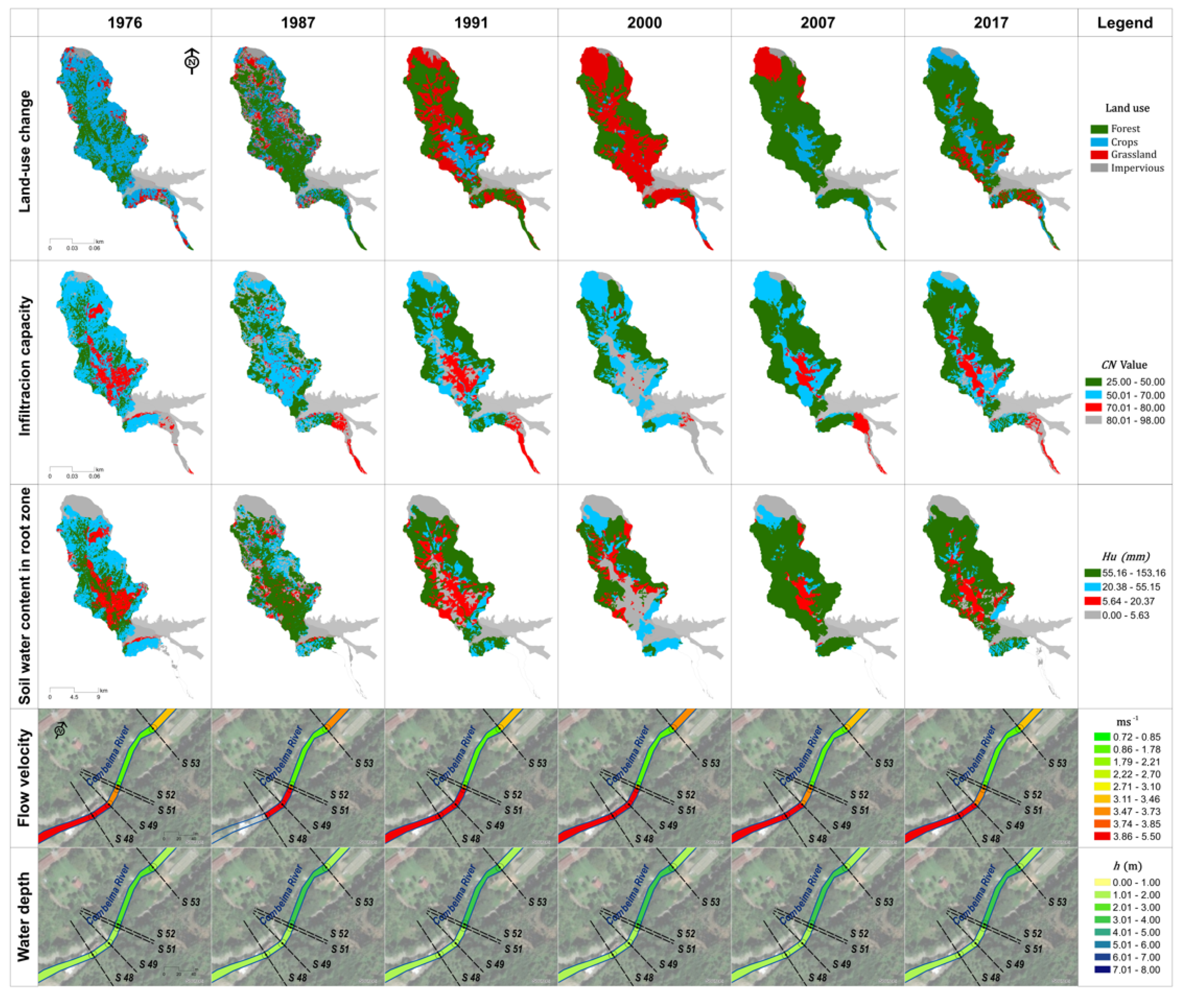
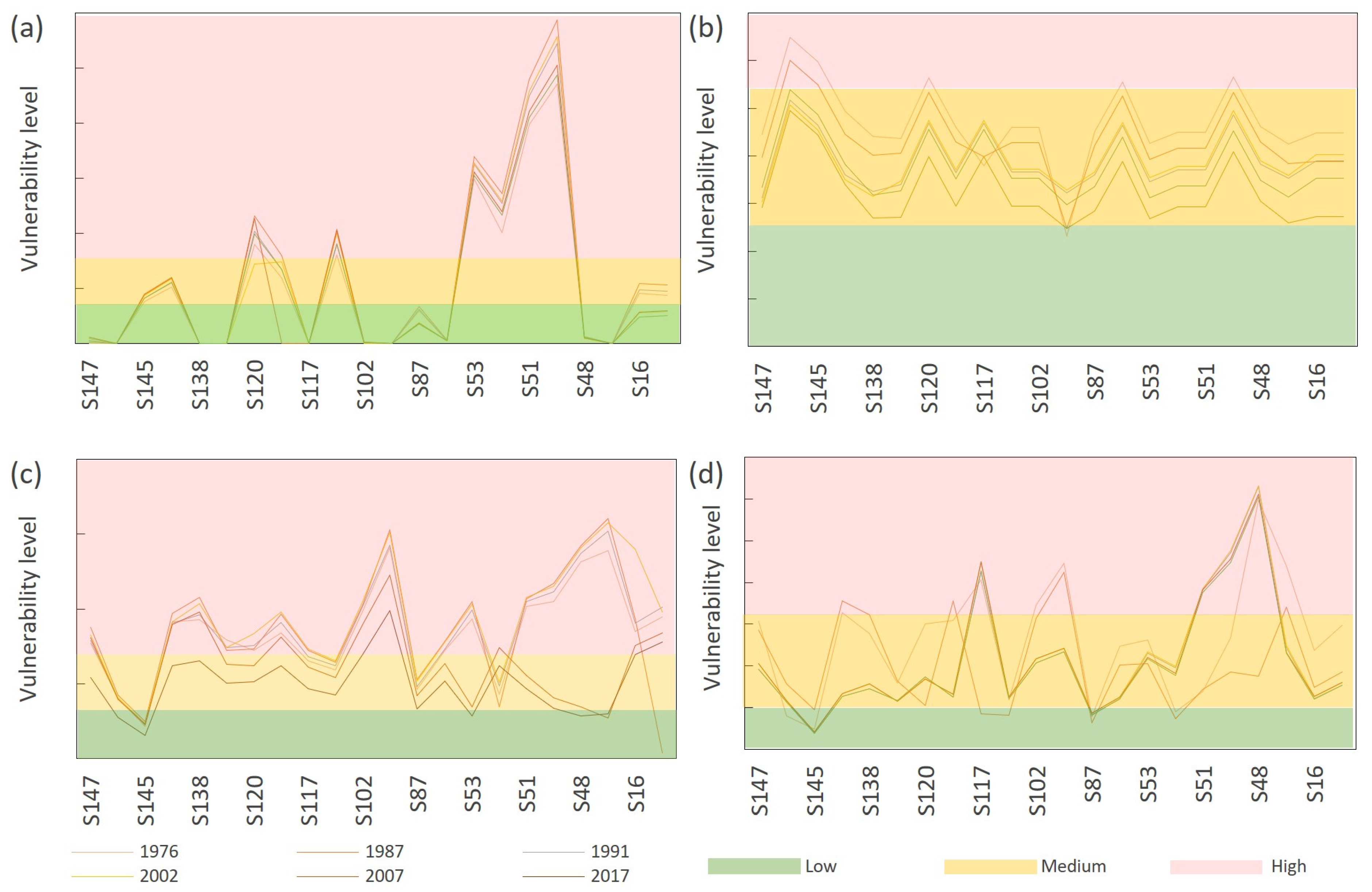
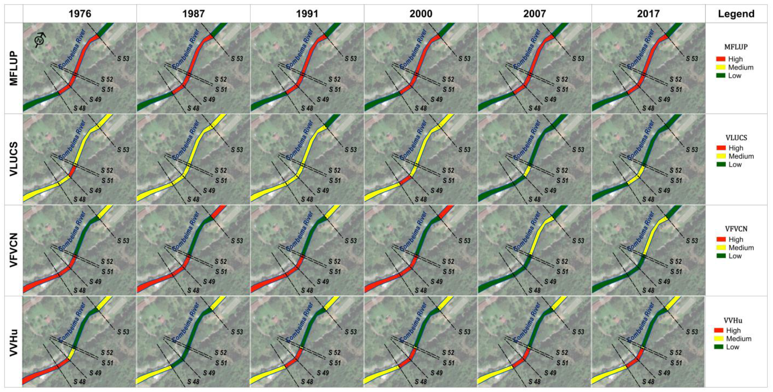
3.3. Effect of Land-Use Change on the Physical Vulnerability

The results of the hydrological and hydraulic modeling allowed the evaluation of the physical vulnerability of exposed structures in land-use change scenarios ($V_{ij}$) by applying the MFLUP, VLUCS, VVHu, and VFVCN methods (

Table 3. Variation of physical vulnerability in the land-use change scenarios evaluated per method.

Cross	Scenario 1976				Scenario 1987				Scenario 1991				Scenario 2000				Scenario 2007				Scenario 2017
Section	MFLUP	VLUCS	VFVCN	VVHu	MFLUP	VLUCS	VFVCN	VVHu	MFLUP	VLUCS	VFVCN	VVHu	MFLUP	VLUCS	VFVCN	VVHu	MFLUP	VLUCS	VFVCN	VVHu	MFLUP	VLUCS	VFVCN	VVHu
147
146
145
144
138
121
120
119
117
103
102
95
87
86
53
52
51
49
48
42
16
15

Notes: Physical vulnerability levels correspond to the following colors: green = low, yellow = medium, and red = high. MFLUP: vulnerability and mapping of floods based on land-use patterns, VLUCS: vulnerability in land-use change scenarios, VFVCN: vulnerability based on flow velocity and curve number, VVHu: vulnerability based on soil water storage variation.

). In the simulated stream reach sections for the years 1976, 2007, and 2017, the levels of physical vulnerability and lower maximum flows are observed, related to the larger areas of forests and crops in the basin. Likewise, the 1987 and 2000 scenarios show the most extensive areas with grassland and impervious surfaces, which produce, as a hydrological response in the basin, the largest magnitudes in the simulated maximum flows and, therefore, the highest estimated physical vulnerabilities in the cross-sections analyzed. This behavior shows consistency in all the methods applied for the land-use scenarios analyzed (Table 3, Figure 4 and Figure 5).

The MFLUP and VFVHu methods showed higher sensitivity to land-use changes in the basin. This is because the first considers area changes per land-use, and the latter integrates soil water storage changes in the root zone and the flow velocity in the cross-section in which the exposed structure is located (Figure 5 and Figure 6).

The VLUCS method did not reflect noticeable changes in the level of vulnerability when modifying the maximum flow and the water depth due to land-use change (Table 2 and Table 3), aspects that define the degree of exposure of the structure concerning the current flow. This result can be attributed to the fact that this method estimates vulnerability based on the slope of the basin, land-use, soil type, and the elevation at which the exposed element is located [26], i.e., it estimates vulnerability based on the basin and its land-use attributes.

The greater capacity of the VVHu method to represent changes in the physical vulnerability of structures exposed to flooding in land-use change scenarios is explained by the fact that it incorporates in its estimation the response of the basin to variations in infiltration capacity and the current flow velocity in the channel. In addition, the structures with greater exposure have higher vulnerability values [54], and this exposure varies according to the land-use evolution in the basin [55,56].

Likewise, physical vulnerability mapping using GIS showed that higher flow velocities are related to high levels of vulnerability (Figure 6), consistent with what was reported by [57,58].

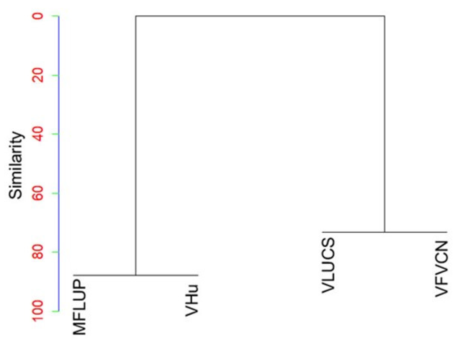
3.4. Analysis of Similarity between Methods

Based on the results obtained from the evaluation of physical vulnerability using four methods in different analysis scenarios, only those cases in which there were coincidences in the levels of vulnerability in each cross-section evaluated were selected for performing an AHC. The analysis indicates that VVHu shows 90% similarity with MFLUP. Likewise, VFVCN presents a similarity of 70% with respect to VLUCS (Figure 7). Therefore, the methods proposed in this paper, i.e., VVHu and VFVCN, exhibit a high similarity in relation to MFLUP and VFVCN [37]. These are based on the vulnerability evaluation concerning the level of exposure of structures near streams and morpho-edaphological characteristics of the basin. Thus, the methods proposed in this research are a new approach to evaluating physical vulnerability since they are based on analyzing the variation of the hydraulic properties of the soil (Hu and CN), and flow velocity ($v$) in the cross-section where the exposed structures are located.

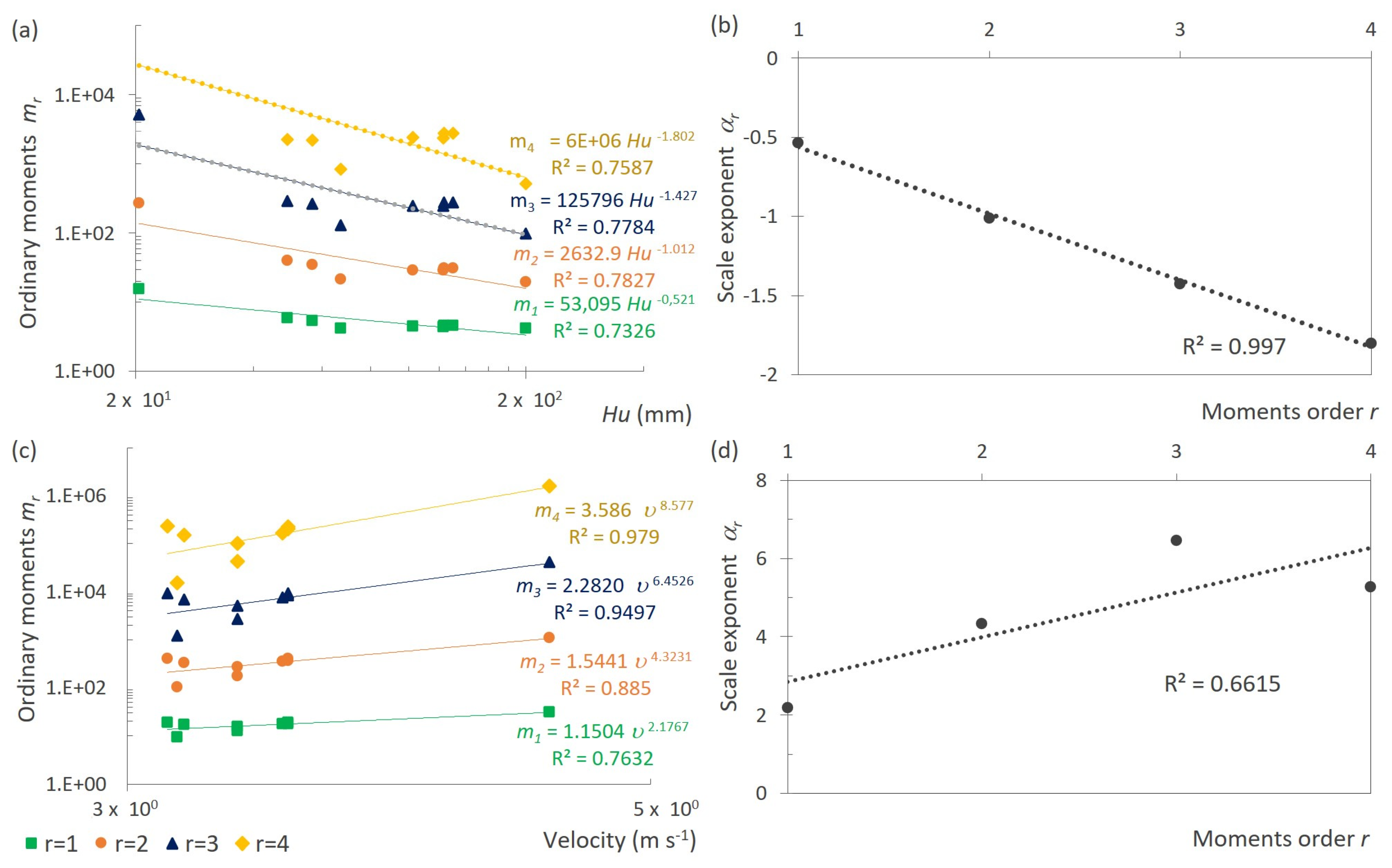
3.5. Scaling Physical Vulnerability in a Land-Use Change Scenario

Logarithms Hu and $v$ with respect to ($V_{ij}$) showed a broad, simple scaling (Figure 8a,c) since they present linearity in order r moments for each scale (Figure 8b,d). Regressions for scale Hu showed R² values between 0.7587 and 0.7647. In the case of scale $v$, R² values varied between 0.5839 and 0.7751. These results indicate that both the current flow velocity and the soil water storage in the root zone represent the effect of land-use change in the basin on the hydraulics of the current (flow) directly in contact with the exposed structures.

Nevertheless, the variables related to current hydraulics could improve the estimation of the physical vulnerability to floods in a land-use change scenario. In this way, it is possible to represent the response of the natural system in a variable land-use scenario in the basin and use it together with the flow velocity to estimate its effect on the physical vulnerability of structures exposed to floods by using the power law and GIS mapping.

4. Conclusions

The findings of this study show that land-use changes affect the magnitude of floods. In particular, the increase in permeable areas produces flood attenuation due to the increase in soil infiltration capacity. Likewise, the decrease in forest and crop cover and the increase in land uses with low infiltration capacity generate increases in peak flow, flow velocity, and water depth in the cross-sections, directly related to the physical vulnerability level of exposed structures.

Under the conditions in which this analysis was carried out, physical vulnerability estimation can be improved by incorporating hydraulic properties of the soil, such as Hu and CN, together with flow variables, such as flow velocity, since they vary with land-use evolution at the basin scale, facilitating the mapping of the physical vulnerability of structures exposed to floods by using GIS. However, the methodology shows limitations since it is necessary to obtain cross-sections of the stream to implement a hydraulic model according to the level of detail required for each case study. In this sense, the manifestation of the WSSS with the incorporation of scales such as Hu, CN, and $v$ contributes to simplifying the process of estimating the physical vulnerability in cross-sections of a stream by projecting land-use variation at the basin scale, given the ease of applying the power law without requiring a hydraulic modeling process. Therefore, this approach could be useful and practical in land-use planning processes in small basins using GIS and could facilitate the prediction of the physical vulnerability of structures close to surface water currents in land-use change scenarios with scarce information.

References

1. WMO. 2018 Annual Report: WMO for the Twenty-First Century, No. 1229. 2018. Available online: https://library.wmo.int/doc_num.php?explnum_id=6264 (accessed on 11 February 2023).
2. Erlick, J.C. Natural Disasters in Latin America and the Caribbean; Routledge: London, UK, 2021. [Google Scholar] [CrossRef]
3. Bhatt, C.; Rao, G.; Diwakar, P.; Dadhwal, V. Development of flood inundation extent libraries over a range of potential flood levels: A practical framework for quick flood response. Geomat. Nat. Hazards Risk 2016, 8, 384–401. [Google Scholar] [CrossRef] [Green Version]
4. Baeck, S.H.; Choi, S.J.; Choi, G.W.; Lee, N.R. A study of evaluating and forecasting watersheds using the flood vulnerability assessment index in Korea. Geomat. Nat. Hazards Risk 2014, 5, 208–231. [Google Scholar] [CrossRef] [Green Version]
5. Ye, B.; Jiang, J.; Liu, J.; Zheng, Y.; Zhou, N. Research on quantitative assessment of climate change risk at an urban scale: Review of recent progress and outlook of future direction. Renew. Sustain. Energy Rev. 2021, 135, 110415. [Google Scholar] [CrossRef]
6. Yang, Y.-C.; Ge, Y.-E. Adaptation strategies for port infrastructure and facilities under climate change at the Kaohsiung port. Transp. Policy 2020, 97, 232–244. [Google Scholar] [CrossRef]
7. Dandapat, K.; Panda, G.K. Flood vulnerability analysis and risk assessment using analytical hierarchy process. Model. Earth Syst. Environ. 2017, 3, 1627–1646. [Google Scholar] [CrossRef]
8. Gain, A.K.; Mojtahed, V.; Biscaro, C.; Balbi, S.; Giupponi, C. An integrated approach of flood risk assessment in the eastern part of Dhaka City. Nat. Hazards 2015, 79, 1499–1530. [Google Scholar] [CrossRef] [Green Version]
9. Marques, G.F.; de Souza, V.B.; Moraes, N.V. The economic value of the flow regulation environmental service in a Brazilian urban watershed. J. Hydrol. 2017, 554, 406–419. [Google Scholar] [CrossRef]
10. Chowdhuri, I.; Pal, S.C.; Chakrabortty, R. Flood susceptibility mapping by ensemble evidential belief function and binomial logistic regression model on river basin of eastern India. Adv. Space Res. 2020, 65, 1466–1489. [Google Scholar] [CrossRef]
11. Haque, M.; Islam, S.; Sikder, B.; Islam, S. Community flood resilience assessment in Jamuna floodplain: A case study in Jamalpur District Bangladesh. Int. J. Disaster Risk Reduct. 2022, 72, 102861. [Google Scholar] [CrossRef]
12. Fernández-Montblanc, T.; Duo, E.; Ciavola, P. Dune reconstruction and revegetation as a potential measure to decrease coastal erosion and flooding under extreme storm conditions. Ocean Coast. Manag. 2019, 188, 105075. [Google Scholar] [CrossRef]
13. Ettinger, S.; Mounaud, L.; Magill, C.; Yao-Lafourcade, A.-F.; Thouret, J.-C.; Manville, V.; Negulescu, C.; Zuccaro, G.; De Gregorio, D.; Nardone, S.; et al. Building vulnerability to hydro-geomorphic hazards: Estimating damage probability from qualitative vulnerability assessment using logistic regression. J. Hydrol. 2016, 541, 563–581. [Google Scholar] [CrossRef]
14. Laudan, J.; Rözer, V.; Sieg, T.; Vogel, K.; Thieken, A.H. Damage assessment in Braunsbach 2016: Data collection and analysis for an improved understanding of damaging processes during flash floods. Nat. Hazards Earth Syst. Sci. 2017, 17, 2163–2179. [Google Scholar] [CrossRef] [Green Version]
15. Guidolin, M.; Chen, A.S.; Ghimire, B.; Keedwell, E.C.; Djordjević, S.; Savić, D.A. A weighted cellular automata 2D inundation model for rapid flood analysis. Environ. Model. Softw. 2016, 84, 378–394. [Google Scholar] [CrossRef] [Green Version]
16. Van Westen, C.J. Remote Sensing and GIS for Natural Hazards Assessment and Disaster Risk Management. In Treatise on Geomorphology; Academic Press: Cambridge, MA, USA, 2013; Volume 3, pp. 259–298. [Google Scholar] [CrossRef]
17. Hendrawan, V.S.A.; Komori, D. Developing flood vulnerability curve for rice crop using remote sensing and hydrodynamic modeling. Int. J. Disaster Risk Reduct. 2021, 54, 102058. [Google Scholar] [CrossRef]
18. Karagiorgos, K.; Thaler, T.; Hübl, J.; Maris, F.; Fuchs, S. Multi-vulnerability analysis for flash flood risk management. Nat. Hazards 2016, 82, 63–87. [Google Scholar] [CrossRef] [Green Version]
19. Bankoff. Mapping Vulnerability: Disasters, Development and People, Earthscan, 1st ed.; Taylor & Francis: London, UK, 2004. [Google Scholar]
20. Gabel, F. Chancen dynamischer Konzeptionen von Vulnerabilität für den Katastrophenschutz. In Resilienz im Katastrophenfall Konzepte zur Stärkung von Pflege- und Hilfsbedürftigen im Bevölkerungsschutz; Marco Krüger, Matthias Max—Bielefeld Transcr: Gnoien, Germany, 2019; pp. 77–96. [Google Scholar]
21. Malik, S.; Pal, S.C.; Sattar, A.; Singh, S.K.; Das, B.; Chakrabortty, R.; Mohammad, P. Trend of extreme rainfall events using suitable Global Circulation Model to combat the water logging condition in Kolkata Metropolitan Area. Urban Clim. 2020, 32, 100599. [Google Scholar] [CrossRef]
22. Blöschl, G. Three hypotheses on changing river flood hazards. Hydrol. Earth Syst. Sci. 2022, 26, 5015–5033. [Google Scholar] [CrossRef]
23. Messner, V.; Meyer, F. Flood Damage, Vulnerability and Risk Perception—Challenges for Flood Damage Research; Springer: Berlin/Heidelberg, Germany, 2005. [Google Scholar]
24. Liu, J.; Shi, Z.; Wang, D. Measuring and mapping the flood vulnerability based on land-use patterns: A case study of Beijing, China. Nat. Hazards 2016, 83, 1545–1565. [Google Scholar] [CrossRef]
25. Wu, F.; Sun, Y.; Sun, Z.; Wu, S.; Zhang, Q. Assessing agricultural system vulnerability to floods: A hybrid approach using emergy and a landscape fragmentation index. Ecol. Indic. 2019, 105, 337–346. [Google Scholar] [CrossRef]
26. Caldas, A.M.; Pissarra, T.C.T.; Costa, R.C.A.; Neto, F.C.R.; Zanata, M.; da Parahyba, R.B.V.; Fernandes, L.F.S.; Pacheco, F.A.L. Flood Vulnerability, Environmental Land Use Conflicts, and Conservation of Soil and Water: A Study in the Batatais SP Municipality, Brazil. Water 2018, 10, 1357. [Google Scholar] [CrossRef] [Green Version]
27. USDA-SCS. Section 4: Hidrology. In National Engineering Handbook; Soil Conservation Service; United States Department of Agriculture: Washington, DC, USA, 1972; p. 127. [Google Scholar]
28. Peña, L.E.; Barrios, M.; Francés, F. Flood quantiles scaling with upper soil hydraulic properties for different land uses at catchment scale. J. Hydrol. 2016, 541, 1258–1272. [Google Scholar] [CrossRef] [Green Version]
29. Saxton, K.E.; Rawls, W.J. Soil Water Characteristic Estimates by Texture and Organic Matter for Hydrologic Solutions. Soil Sci. Soc. Am. J. 2006, 70, 1569–1578. [Google Scholar] [CrossRef] [Green Version]
30. Soil Survey Staff. Soil Taxonomy, 2nd ed.; U.S. Government Printing Office: Washington, DC, USA, 1999. [Google Scholar]
31. United States Departament of Agriculture. Keys to Soil Taxonomy; SMSS Technical monograph No. 19; Pocahontas Press, Inc.: Blacksburg, VA, USA, 1992. [Google Scholar]
32. Francés, F.; Vélez, J.I.; Vélez, J.J. Split-parameter structure for the automatic calibration of distributed hydrological models. J. Hydrol. 2007, 332, 226–240. [Google Scholar] [CrossRef]
33. Medici, C.; Butturini, A.; Bernal, S.; Vázquez, E.; Sabater, F.; Vélez, J.I.; Francés, F. Modelling the non-linear hydrological behaviour of a small Mediterranean forested catchment. Hydrol. Process. 2008, 22, 3814–3828. [Google Scholar] [CrossRef]
34. Salazar, S.; Francés, F.; Komma, J.; Blume, T.; Francke, T.; Bronstert, A.; Bloschl, G. A comparative analysis of the effectiveness of flood management measures based on the concept of “retaining water in the landscape” in different European hydro-climatic regions. Nat. Hazards Earth Syst. Sci. 2012, 12, 3287–3306. [Google Scholar] [CrossRef] [Green Version]
35. Francésa, F.; Bussib, G. Análisis del impacto del cambio climático en el ciclo de sedimentos de la cuenca del río Ésera (España) mediante un modelo hidrológico distribuido. Rev. Iberoam. Ribagua 2014, 1, 14–25. [Google Scholar] [CrossRef] [Green Version]
36. Siswanto, S.Y.; Francés, F. How land use/land cover changes can affect water, flooding and sedimentation in a tropical watershed: A case study using distributed modeling in the Upper Citarum watershed, Indonesia. Environ. Earth Sci. 2019, 78, 550. [Google Scholar] [CrossRef]
37. Teng, J.; Jakeman, A.J.; Vaze, J.; Croke, B.F.W.; Dutta, D.; Kim, S. Flood inundation modelling: A review of methods, recent advances and uncertainty analysis. Environ. Model. Softw. 2017, 90, 201–216. [Google Scholar] [CrossRef]
38. Bozzi, S.; Passoni, G.; Bernardara, P.; Goutal, N.; Arnaud, A. Roughness and Discharge Uncertainty in 1D Water Level Calculations. Environ. Model. Assess. 2014, 20, 343–353. [Google Scholar] [CrossRef]
39. Liu, J.; Shi, Z.; Tan, X. Measuring the dynamic evolution of road network vulnerability to floods: A case study of Wuhan, China. Travel Behav. Soc. 2020, 23, 13–24. [Google Scholar] [CrossRef]
40. Ologunorisa, T.E. An assessment of flood vulnerability zones in the Niger delta, Nigeria. Int. J. Environ. Stud. 2004, 61, 31–38. [Google Scholar] [CrossRef]
41. Sokal, R.R.; Michener, C.D. A statistical method for evaluating systematic relationships. Univ. Kansas Sci. Bull. 1958, 38, 1409–1438. [Google Scholar]
42. Huang, L.; Wang, G.; Wang, Y.; Blanzieri, E.; Su, C. Link Clustering with Extended Link Similarity and EQ Evaluation Division. PLoS ONE 2013, 8, e66005. [Google Scholar] [CrossRef] [PubMed]
43. Xu, H.; Ma, C.; Lian, J.; Xu, K.; Chaima, E. Urban flooding risk assessment based on an integrated k-means cluster algorithm and improved entropy weight method in the region of Haikou, China. J. Hydrol. 2018, 563, 975–986. [Google Scholar] [CrossRef]
44. Burlando, P.; Rosso, R. Scaling and muitiscaling models of depth-duration-frequency curves for storm precipitation. J. Hydrol. 1996, 187, 45–64. [Google Scholar] [CrossRef]
45. Moriasi, D.N.; Arnold, J.G.; van Liew, M.W.; Bingner, R.L.; Harmel, R.D.; Veith, T.L. Model evaluation guidelines for systematic quantification of accuracy in watershed simulations. Trans. ASABE 2007, 50, 885–900. [Google Scholar] [CrossRef]
46. Kundu, S.; Khare, D.; Mondal, A. Individual and combined impacts of future climate and land use changes on the water balance. Ecol. Eng. 2017, 105, 42–57. [Google Scholar] [CrossRef]
47. Marshall, M.R.; Ballard, C.E.; Frogbrook, Z.L.; Solloway, I.; McIntyre, N.; Reynolds, B.; Wheater, H.S. The impact of rural land management changes on soil hydraulic properties and runoff processes: Results from experimental plots in upland UK. Hydrol. Process. 2014, 28, 2617–2629. [Google Scholar] [CrossRef]
48. GEOTEC. Estudio de Amenazas Naturales, Vulnerabilidad y Escenarios de Riesgo en los Centros Poblados de Villarestrepo, Llanitos, Juntas, Pastales, Pico de Oro, Bocatoma Combeima y Cay, por Flujos Torrenciales en las Microcuencas del Río Combeima; Geotec Group—Alcaldía de Ibagué—Cortolima: Ibagué, Colombia, 2007. [Google Scholar]
49. Alaoui, A.; Rogger, M.; Peth, S.; Blöschl, G. Does soil compaction increase floods? A review. J. Hydrol. 2018, 557, 631–642. [Google Scholar] [CrossRef]
50. Odunuga, S.; Adegun, O.; Raji, S.A.; Udofia, S. Changes in flood risk in Lower Niger–Benue catchments. Proc. Int. Assoc. Hydrol. Sci. 2015, 370, 97–102. [Google Scholar] [CrossRef] [Green Version]
51. Jobe, A.; Kalra, A.; Ibendahl, E. Conservation Reserve Program effects on floodplain land cover management. J. Environ. Manag. 2018, 214, 305–314. [Google Scholar] [CrossRef] [PubMed]
52. Horton, A.J.; Nygren, A.; Diaz-Perera, M.A.; Kummu, M. Flood severity along the Usumacinta River, Mexico: Identifying the anthropogenic signature of tropical forest conversion. J. Hydrol. X 2020, 10, 100072. [Google Scholar] [CrossRef]
53. Andréassian, V. Waters and forests: From historical controversy to scientific debate. J. Hydrol. 2004, 291, 1–27. [Google Scholar] [CrossRef]
54. Tanir, T.; Sumi, S.J.; Lima, A.D.S.D.; Coelho, G.D.A.; Uzun, S.; Cassalho, F.; Ferreira, C.M. Multi-scale comparison of urban socio-economic vulnerability in the Washington, DC metropolitan region resulting from compound flooding. Int. J. Disaster Risk Reduct. 2021, 61, 102362. [Google Scholar] [CrossRef]
55. Czech, W.; Radecki-Pawlik, A.; Wyżga, B.; Hajdukiewicz, H. Modelling the flooding capacity of a Polish Carpathian river: A comparison of constrained and free channel conditions. Geomorphology 2016, 272, 32–42. [Google Scholar] [CrossRef]
56. McEachran, Z.P.; Karwan, D.L.; Sebestyen, S.D.; Slesak, R.A.; Ng, G.-H.C. Nonstationary flood-frequency analysis to assess effects of harvest and cover type conversion on peak flows at the Marcell Experimental Forest, Minnesota, USA. J. Hydrol. 2021, 596, 126054. [Google Scholar] [CrossRef]
57. Zhao, L.; Liu, F. Land-use planning adaptation in response to SLR based on a vulnerability analysis. Ocean Coast. Manag. 2020, 196, 105297. [Google Scholar] [CrossRef]
58. Rahman, M.; Ningsheng, C.; Mahmud, G.I.; Islam, M.; Pourghasemi, H.R.; Ahmad, H.; Habumugisha, J.M.; Washakh, R.M.A.; Alam, M.; Liu, E.; et al. Flooding and its relationship with land cover change, population growth, and road density. Geosci. Front. 2021, 12, 101224. [Google Scholar] [CrossRef]
Figure 1. Location of the study area.
Water 15 01214 g001
Figure 2. Hydrological modeling: (a) calibration period: 1984–1985, (b) validation period: 2017–2018, (c) hydraulic model calibration, (d) Manning’s n coefficient values adopted in the simulated stream reach.
Water 15 01214 g002
Figure 3. Hydrological response by land–use change period. (a) land–use areas, (b) annual maxima, and (c) flood quantiles.
Water 15 01214 g003
Figure 4. Simulated variations of land-use change, soil infiltration capacity (CN), soil water content in the root zone (Hu), stream flow velocity ( v ), and water depth ( h ) (in order, from top to bottom) related to land-use change during the 1976–2017 period in sections S48–S53 located in the lower part of the stream reach analyzed.
Water 15 01214 g004
Figure 5. Evaluation of the physical vulnerability to floods by applying the following methods: (a) vulnerability and mapping of floods based on land-use patterns (MFLUP); (b) vulnerability in land-use change scenarios (VLUCS); (c) vulnerability based on flow velocity and curve number (VFVCN); and (d) vulnerability based on soil water storage variation (VVHu).
Water 15 01214 g005
Figure 6. Changes in physical vulnerability in the 1976–2017 period applying the four methods analyzed. MFLUP: vulnerability and mapping of floods based on land-use patterns; VLUCS: vulnerability in land-use change scenarios; VFVCN: vulnerability based on flow velocity and curve number; VVHu vulnerability based on soil water storage variation.
Water 15 01214 g006
Figure 7. Dendrogram of similarity of the methods used in this study to assess the physical vulnerability of structures.
Water 15 01214 g007
Figure 8. Scalable behavior manifestation of physical vulnerability with respect to (a) soil water storage variation in the root zone (Hu) and (c) stream flow velocity variation ( v ). Linearity of scale exponents with (b) Hu variation and (d) v variation.
Water 15 01214 g008