Groundwater Quality and Health Risk Assessment Using Indexing Approaches, Multivariate Statistical Analysis, Artificial Neural Networks, and GIS Techniques in El Kharga Oasis, Egypt

Abstract

The assessment and prediction of water quality are important aspects of water resource management. Therefore, the groundwater (GW) quality of the Nubian Sandstone Aquifer (NSSA) in El Kharga Oasis was evaluated using indexing approaches, such as the drinking water quality index (DWQI) and health index (HI), supported with multivariate analysis, artificial neural network (ANN) models, and geographic information system (GIS) techniques. For this, physical and chemical parameters were measured for 140 GW wells, which indicated Ca–Mg–SO₄, mixed Ca–Mg–Cl–SO₄, Na–Cl, Ca–Mg–HCO₃, and mixed Na–Ca–HCO₃ water facies under the influence of silicate weathering, rock–water interactions, and ion exchange processes. The GW in El Kharga Oasis had high levels of heavy metals, particularly iron (Fe) and manganese (Mn), with average concentrations above the limits recommended by the World Health Organization (WHO) for drinking water. The DWQI categorized most of the samples as not suitable for drinking (poor to very poor class), while some samples fell in the good water class. The results of the HI indicated a potential health risk due to the ingestion of water, with the risk being higher for children in only one location. However, for both children and adults, there was a low risk of dermal and ingestion exposure to the water in all locations. The contaminants could be from natural sources, such as minerals leaching from rocks and soil, or from human activities. Based on the results of ANN modeling, ANN-SC-13 was the most accurate prediction model, since it demonstrated the strongest correlation between the best characteristics and the DWQI. For example, this model’s thirteen characteristics were extremely important for predicting DWQI. The R² value for the training, cross-validation (CV), and test data was 0.99. The ANN-SC-2 model was the best in measuring HI ingestion in adults. The R² value for the training, CV, and test data was 1.00 for all models. The ANN-SC-2 model was the most accurate at detecting HI dermal in adults (R² = 0.99, 0.99, and 0.99 for the training, CV, and test data sets, respectively). Finally, the integration of physicochemical parameters, water quality indices (WQIs), and ANN models can help us to understand the quality of GW and its controlling factors, and to implement the necessary measures that prevent outbreaks of various water-borne diseases that are detrimental to human health.

1. Introduction

Freshwater supply for drinking purposes in arid and semiarid regions worldwide relies heavily on GW, as it is the most crucial source [1,2]. Although the provision of clean and adequate water is deemed a basic human entitlement, the standard of GW is diminishing in numerous regions worldwide due to the scarcity of water [3,4,5]. The concentration of hydrochemical parameters in GW is influenced by a variety of geochemical processes that occur through the interaction of rocks and water [6]. Consequently, researchers worldwide have been focusing on understanding the primary processes controlling major hydrochemical ions in GW, as well as evaluating the potential risks of GW pollution to human health and the natural environment. In the past few years, various studies have been carried out to scrutinize the hydrogeochemical traits and quality of GW [7,8,9,10,11,12]. In addition to major hydrochemical ions, the quality of GW is influenced by many physicochemical constituents, including natural and human-caused pollutants [13,14]. Unfortunately, as civilization has progressed, the quality of GW has deteriorated significantly because of natural and human-induced activities, which have adversely impacted the hydrogeological environment and human health [15]. In recent decades, Egypt has experienced a significant increase in water demand due to population growth and increased agricultural production. El Kharga Oasis is one of several oases located in the New Valley Governorate of Egypt. However, it is important to note that the population of each individual oasis within the governorate is not typically reported separately [16]. The primary source of drinking water in El Kharga Oasis is GW, which varies in depth depending on the location within the oasis. The depth of the GW varies depending on the location within the oasis, with some areas having shallow GW while others require deeper drilling to access water. According to a study on water resource management in El Kharga Oasis, the average depth of the GW in the oasis is around 500 m. The per capita consumption of water in the oasis is relatively low compared to the national average, but there are concerns about the sustainability of water use due to population growth and development. Wastewater collection and treatment systems are limited in scope, with some untreated wastewater being discharged into the environment, which could be a potential source of pollution in El Kharga Oasis [17]. However, the increase in population has led to a surge in GW demand, which has caused problems, such as excessive abstraction, leading to declines in GW levels and increased salinity in the NSSA. To address these issues and promote sustainable GW use, various GW management plans have been developed. It is also necessary to evaluate the hydrogeological and hydrochemical properties of the aquifer to improve management practices and protect the GW resources. Inadequate GW management practices in the western desert have made the aquifers susceptible to exploitation, resulting in over 20% of natural recharge being lost under the arid conditions in the region. Therefore, obtaining baseline hydrogeological and hydrogeochemical data for the region is critical for promoting sustainability and protecting GW resources [18].

Having access to a reliable and safe water source is essential for the establishment of a stable community [19]. Nowadays, water pollution is one of the most important environmental issues that the world is facing [20,21,22,23]. Water contamination, a significant concern worldwide, is caused by heavy metals, toxic waste, and anthropogenic effluents from industrialization that pollute surface water and GW [24,25]. These pollutants have adverse effects on human health and the environment, affecting the food chain and terrestrial and aquatic living beings [26,27,28]. The ongoing monitoring of water quality, at both the supply source and the consumer end, is crucial to create a database that combines general and chemical water characteristics and to significantly reduce health hazards [29,30].

A hydrogeochemical study involves analyzing geochemical data using charts, such as piper diagrams, Gibbs diagrams, and ionic relations, to identify the geochemical processes that affect water chemistry and to determine changes in hydrochemical properties. The assessment of WQIs is regarded as the most effective technique to gauge the suitability of water for a particular purpose. WQIs are numeric values calculated based on physical, chemical, and biological parameters found in GW. Using WQIs to classify water quality, specifically with DWQI and HI, is more efficient than traditional methods that compare detected parameters to a given water quality standard [11,31,32]. Combining WQIs with GIS techniques is the most accurate way to describe changes in GW facies [33]. Additionally, multivariate statistical methods are widely used to evaluate GW quality and identify natural and artificial sources of GW pollution.

Although various indices have been created to determine the water’s appropriateness for human consumption, they each possess certain disadvantages that restrict their widespread usefulness. Long-term exposure to Fe and Mn in some areas due to increased GW consumption has been related with harmful impacts on health. Fe and Mn are naturally occurring metals that often coexist in GW due to their shared chemical properties, such as a similar valence charge in physiological conditions, ionic radius, and absorptive mechanisms. Fe and Mn are necessary elements for healthy body function. The WHO [34] has produced aesthetic-based water guidelines for iron at 0.3 mg/L and a health-based drinking water guideline value for manganese of 0.4 mg/L. Mn is frequently present in foods, and few people are deficient in it. Typically, dietary Mn intake is much higher than the amount obtained from drinking water. However, excessive exposure to these metals can increase the risk of developing diseases such as Parkinson’s disease, cardiovascular disease, pigmentation changes, and kidney, liver, and neurological disorders [35,36,37].

When examining the chemical variations in GW, it is essential to highlight multivariate analysis techniques such as cluster analysis (CA) and principal component analysis (PCA) [12,38]. CA and PCA can be used to identify significant physicochemical properties as well as the relationships between these variables, allowing researchers to better understand the key variables influencing the distribution of physicochemical parameters in water [12,39]. Factor analysis (FA) can be applied to examine the geochemical evolution, mineralization, and potential contamination of GW. Furthermore, Roubil [40] employed CA to appraise hydrochemical data. This method is frequently utilized by researchers to examine the chemical progression of GW along its flow [41]. By utilizing this approach, it is feasible to validate variations in space and time attributed to natural and anthropogenic components [41].

Using traditional methods to assess health risk and drinking water quality typically takes time and requires numerous processes to produce the desired results. However, by forecasting and assessing these indices using physical factors as features, machine learning (ML) systems can circumvent this problem. Due to its usefulness in identifying a solution to a difficult problem and highlighting the relationship between input and output data, ML approaches have recently been popular for monitoring water quality in many research projects. Model-based feature selection techniques are commonly used to decide which traits have the best predictive and discriminative abilities [42], which can improve model performance by removing unnecessary features and preventing overfitting. This method also helps in retaining the original feature representation, thus, enhancing interpretability [43]. As such, feature selection methods are increasingly being employed in prediction and modeling tasks [44]. Different methods have been suggested to decrease the dimensionality of data [45], which is determined by the weighted regression coefficient of each variable in the PLS model. Random forest (RF) and decision tree (DT) techniques also rank variables based on relevance [46]. Other approaches, such as the back-propagation neural network index [47] and the adjustment of hyperparameters, have been developed to improve ML model performance [48], ensure scientific study repeatability and fairness [49], and refine prediction models [50]. By modifying hyperparameters, the accuracy of quality parameter prediction can be significantly enhanced for the parameters under investigation.

The main aims of this research study were (i) to describe the chemical composition of GW, its categories, and the processes that control its geochemistry using physicochemical parameters and modeling techniques; (ii) to assess the suitability of GW for drinking purposes and potential health hazards using DWQI and HI; and (iii) to evaluate the accuracy of ANN models in predicting the DWQI and HI for the GW in El Kharga Oasis.

In this work, geochemical characteristics of the GW across the NSSA in El Kharga Oasis were identified using physicochemical parameters and the GW quality was assessed using WQIs. Moreover, an ML model was applied to examine their efficiency in the assessment of GW suitability for drinking and its health risk. The novelty of the present work is to increase the credibility of the integration between WQIs and ANN models in GW resources. Therefore, the integration of physicochemical parameters, WQIs, and multivariate analysis, supported with an ML model and GIS techniques is an important context for identifying GW quality and the geochemical processes controlling it. Therefore, the implemented approach model structure is almost stable, accurate and efficienct for water resource assessment and management.

2. Materials and Methods

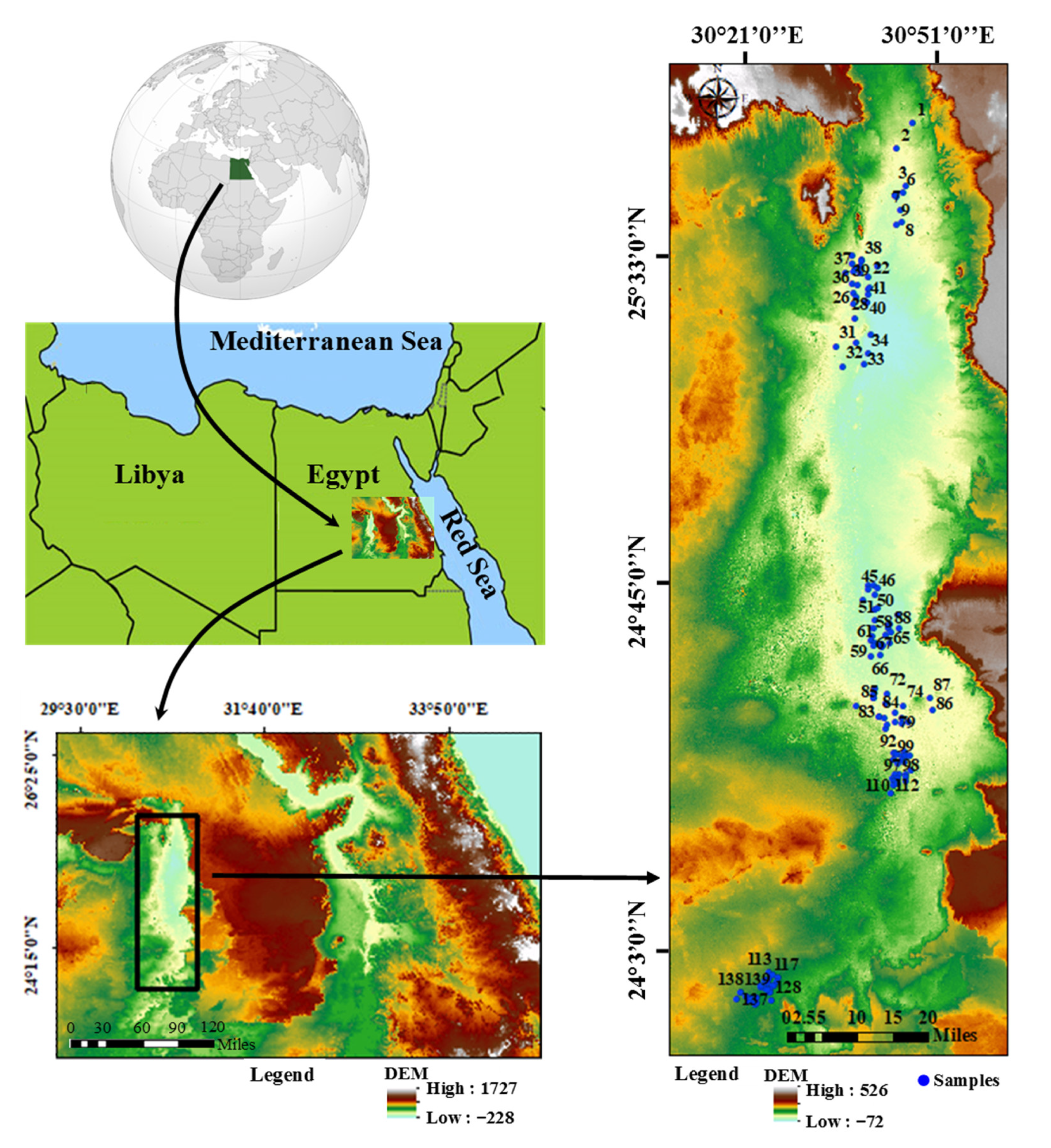
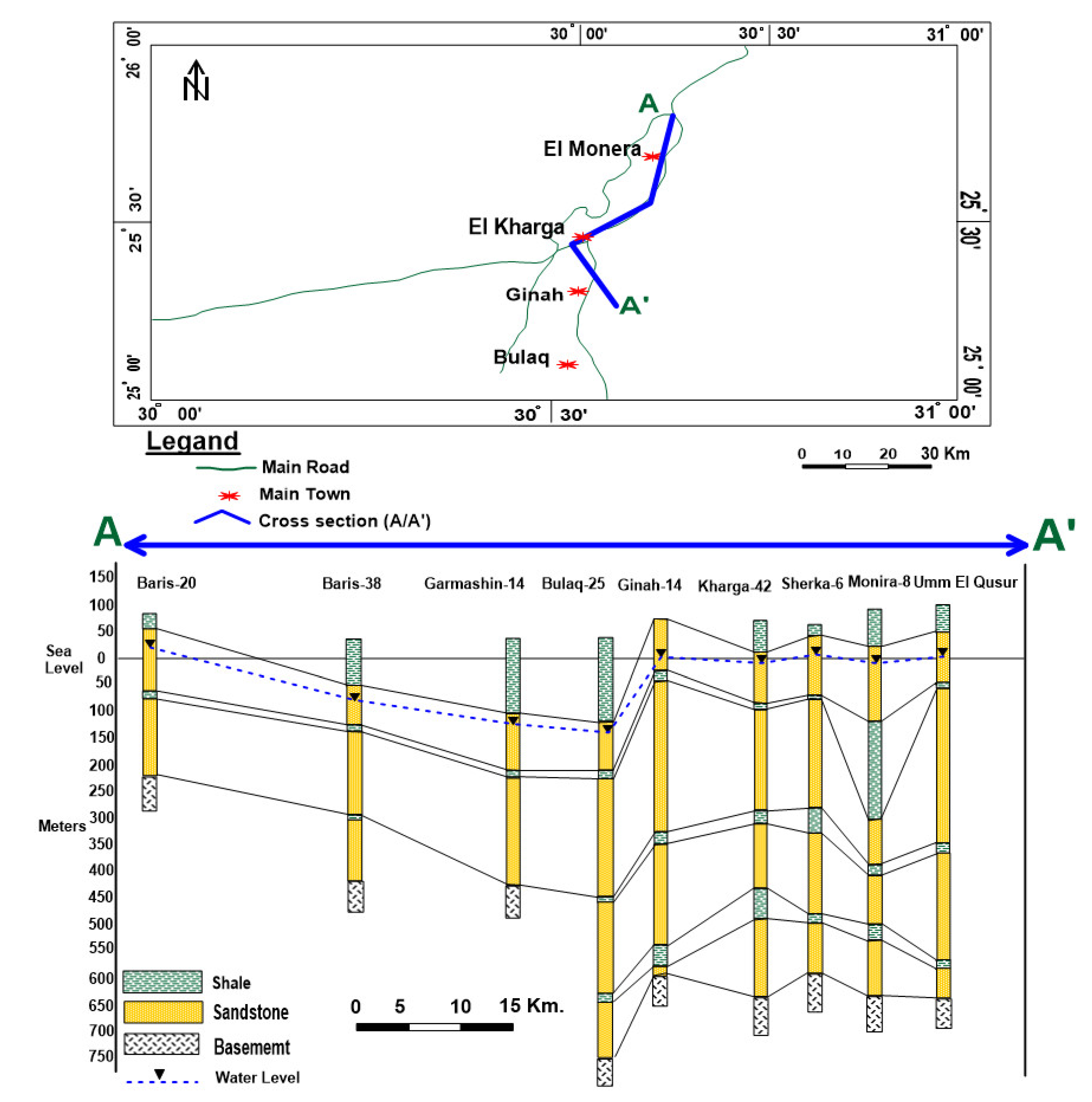
2.1. Description of the Site and Hydrogeological Characteristics

The El Kharga Oasis is a valley in the southern part of the Western Desert, approximately 200 km west of the Nile (Figure 1), with a population of approximately 239,000 people according to the Central Agency for Public Mobilization and Statistics in 2017. The valley is formed by an anticline stretching from north to south, linked to fault zones, with elevations ranging from 0 to 120 m [51]. This region is considered one of the driest locations in the Eastern Sahara and is possibly the most arid area on Earth [52]. The winter season is relatively mild, with temperatures dropping below freezing at night, while the summer is extremely hot, often reaching over 40 °C. Although rainfall is typically less than 1 mm annually, there are rare heavy storms [53,54]. El Kharga Oasis is an agricultural community that cultivates approximately 11,400 hectares of farmland, with date palms being the primary cash crop, along with olives and other fruits [55]. The GW is extracted for drinking and irrigation from 1100 shallow producer wells, producing a total of 8.3 × 10⁶ million cubic meters per year, and approximately 300 government wells, producing 198.1 × 10⁶ m³/y. The wells are dispersed throughout the area, but most are concentrated around major sites, such as El Kharga, Paris, Ghormachine, and Darb Elarbien, with GW depths ranging from 8 to 75 m, as indicated in Figure 2 [56].

The study site is located between 24°00′ and 25°48′ N and 30°100′ and 30°48′ E, as depicted in Figure 1. The Quseir Formation, made up of Upper Cretaceous sediments (NSSA), is present in a considerable part of the study area, predominantly in the east where the other formations of the lower NSSA are not included in the current study. Transmissivity values (T) of El Kharga Oasis range between 100 and 1475 m²/day, with an average value 787.5 m²/day [56]. It is underlaid by Tertiary deposits consisting of marly and chalky limestones, which occur only in the northeast. In the western section of the study region, sand dunes and sabkha sediments with a thickness from 2 to 10 m are prevalent. Additionally, the exposed Precambrian basement rocks (granites) can be seen in the southeastern part of the area. The Nubian Aquifer System (NAS) encompasses four countries and covers a vast land area (Egypt, Sudan, Libya, and Chad) [18,55,57].

The research was carried out in an area where GW flows mainly in a northerly to northeasterly direction, although various flow directions have been recorded. In the northern section of the region, the GW flows from the southwest to the east, while in the central part it flows from the west to the east. In the southern part, localized flow from the south to the northeast was observed. Over-pumping and quick depletion of GW resulted in significant reductions in GW levels in certain regions. The hydraulic gradient in the research area is high, which is likely due to the high rates of GW extraction, the relatively narrow saturation thickness of the Nubian aquifer, and the low hydraulic conductivity of the sediments [58]. The GW aquifer in Baris Oasis and the southern area of the NAS is unconfined, while it is confined in El Kharga Oasis. The thickness of the aquifer gradually increases from north to south. The study also found that the Nubian Sandstone lies above basement rocks and is divided by thin shale layers, which could be interconnected through fault zones. Excessive exploitation of GW in the region may lead to substantial declines in aquifer potentiometric head and degradation of water quality [9].

2.2. Sampling and Analytical Methods

In July 2020, a total of 140 production wells were sampled to collect GW samples from the Nubian sandstone aquifer. In the field, measurements were conducted for parameters including ground surface elevation, EC, temperature, and pH. To measure EC and pH, a mobile multimeter (HI 9829 type) was utilized. The GW samples were divided into two categories, filtered, and then placed in polyethylene bottles and stored in a refrigerator with a temperature of 4 °C. For Fe and Mn analysis, the first group was acidified using HNO₃ until pH < 2, while the second group was used for analyzing Ca²⁺, Mg²⁺, Na⁺, K⁺, Cl⁻, HCO₃⁻, CO₃²⁻, and SO₄²⁻. Spectrophotometer HACH (DR2000 type) was employed to conduct an analysis of SO₄²⁻ and Cl⁻, while flame spectrophotometer was utilized for analyzing K⁺, Ca⁺, and Na⁺. The titrimetric methodology was employed to measure CO₃²⁻ and HCO₃⁻ while the complexometric approach was used to measure Mg²⁺. Additionally, atomic absorption spectrometer (FAAS-Zeeman AASZ-5000, Hitachi, Japan) was used to analyze Fe and Mn concentrations. To verify the analytical precision of the measured ion concentrations in meq/L, equation 1 was used to determine the charge-balance error (CBE), with a set threshold of 5%.

$$\mathrm{CBE}=\frac{\sum \mathrm{Cations}-\sum \mathrm{Anions}}{\sum \mathrm{Cations}+\sum \mathrm{Anions}}\times 100$$

(1)

To ensure the quality of the analytical procedures, appropriate calibrations of the devices were performed and the precision of each sample analyzed was evaluated.

2.3. Multivariate Statistical Methods and Data Treatments

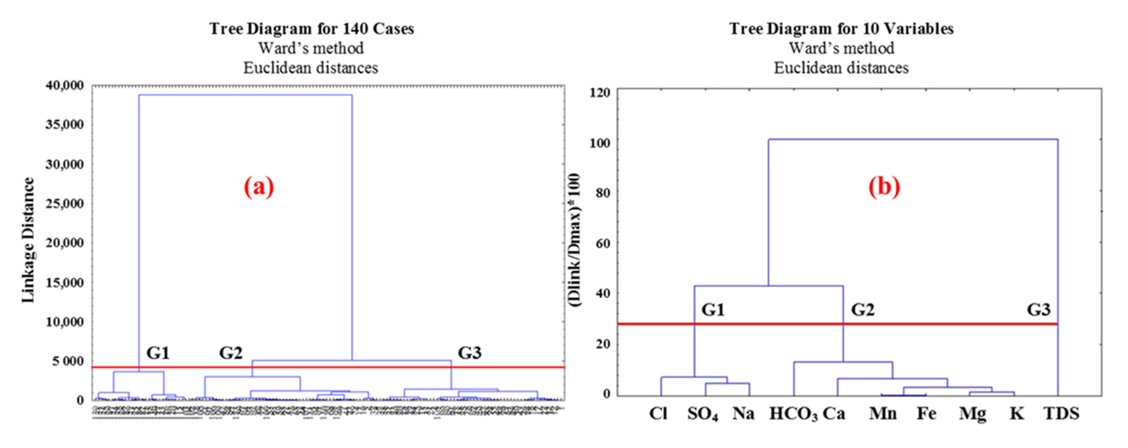
2.3.1. Cluster Analysis (CA)

The technique of CA involves unsupervised pattern recognition, where it identifies key features of different groups by clustering massive datasets from each entity. Both R-mode and Q-mode CA have been used to execute and build a CA. The development and fusion of homogenous groups of water samples into meaningful clusters, as well as the determination of spatial similarity and location clustering within the sampling stations, have all been accomplished using these methodologies. This allows for the grouping of data into distinct clusters [59,60,61]. It is frequently used to categorize hydrogeochemical processes in GW, especially for hydrochemistry investigations, by grouping collected water samples into significant geological and hydrogeological groups [62,63]. A visual representation of the clustering process was provided through the use of a cluster dendrogram. This method displays the groupings and their proximity while significantly reducing the complexity of the original data [64].

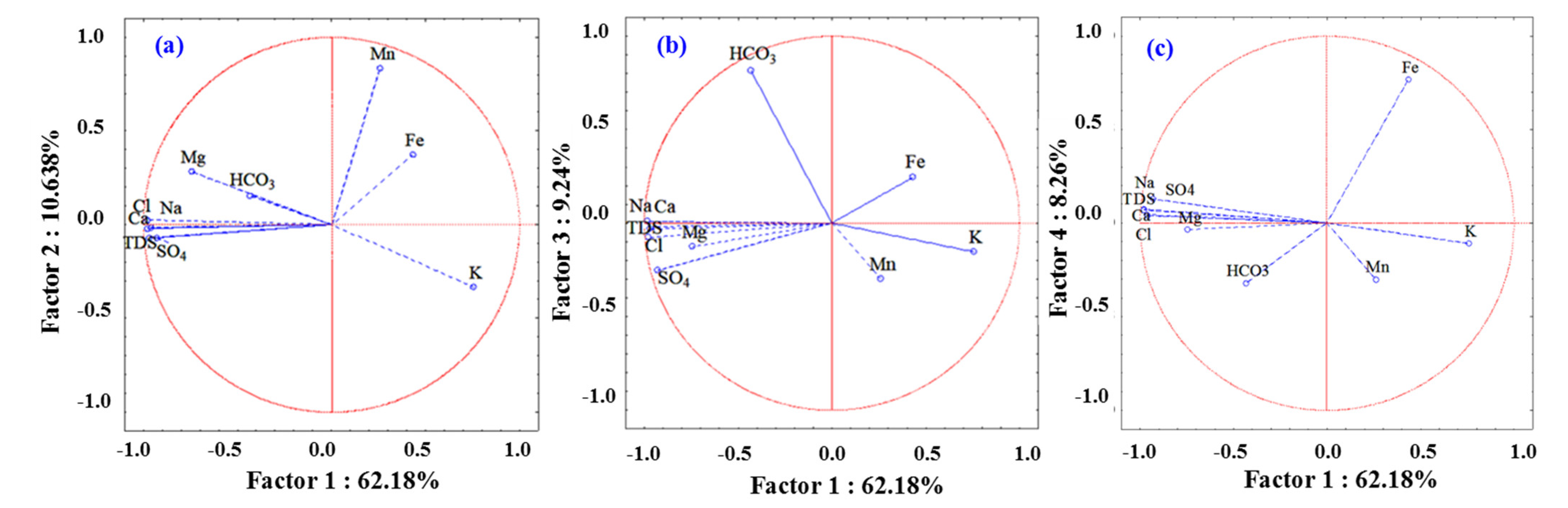
2.3.2. Principal Component Analysis (PCA)

PCA is a linear structure with complex multivariate datasets technique that may be effectively analyzed statistically without information loss [65]. Data may be summarized using principal component analysis, which also provides an estimate of the number of variables needed to account for the observed variance. PCA was applied to reduce the number of variables while still revealing the same level of associated variability [66]. As a result, PCA is a useful approach for understanding the relationships between data pertaining to basic, indirectly visible features [67]. The Kaiser Criterion of the eigenvalue of the scree plot was used to extract the principal components of GW contamination [68]. Data appropriateness for factor analysis, which assesses sample adequacy for each individual variable in the model, was measured using the KMO and Bartlett’s tests. KMO levels between 0.8 and 1, 0.5 and 0.8, and less than 0.5 were regarded as sufficient, fairly adequate, and undesirable or not adequate, respectively [69].

2.4. Indexing Approach

2.4.1. Drinking Water Quality Index (DWQI)

The mathematical techniques used to measure the overall quality of GW for drinking purposes is called the DWQI, which is the most effective method for this purpose [70]. The DWQI is computed using the arithmetic weight approach, as described in Equation (2):

$$\mathrm{DWQI}={{\displaystyle \sum }}_{\mathrm{i}=1}^{\mathrm{n}}{\mathrm{Q}}_{\mathrm{i}}{\mathrm{W}}_{\mathrm{i}}$$

(2)

where Q_i is the sub-quality index of each parameter, and W_i is each parameter’s weight unit. Thirteen physicochemical characteristics (n = 13), given in mg/L, were employed. According to the WHO [34], the estimated value of Q_i depends on the actual concentration (C_i) and standard (S_i) for each physical and chemical characteristic of drinking water, as seen in Equation (3):

$${\mathrm{Q}}_{\mathrm{i}}=\frac{{\mathrm{C}}_{\mathrm{i}}}{{\mathrm{S}}_{\mathrm{i}}}\times 100$$

(3)

$$W_i=\frac{wi}{\sum wi}$$

(4)

W_i was determined for each parameter using Equation (5) in accordance with the suggested criteria [34].

w_i = K/S_i

(5)

where K represents the proportionality constant.

In order to calculate the DWQI, weights must be initially assigned to each GW parameter (w_i), and relative weight (W_i) and quality rating range (Q_i) values must be determined. To accomplish this, W_i values were assigned for various factors, such as pH, EC, TDS, K⁺, Na⁺, Ca⁺², Mg²⁺, alkalinity, Cl⁻, SO₄²⁻, Fe, and Mn, and w_i was computed using Equation (5). These weights were given based on the relative significance of each parameter to drinking water quality, with a range from 2 to 5. The w_i and W_i for each GW parameter are shown in

Table 1. The calculated values of the DWQI based on the relative weights assigned.

Parameter	Weight (wi)	WHO 2017 (mg/L)	Relative Weight (Wi)
pH	3	8.5	0.076923077
EC	5	1500	0.128205128
TDS	5	500	0.128205128
K+	2	12	0.051282051
Na+	3	200	0.076923077
Ca2+	2	50	0.051282051
Mg2+	2	75	0.051282051
Cl−	3	250	0.076923077
SO42−	4	250	0.102564103
HCO3−	2	120	0.051282051
CO32−	2	350	0.051282051
Fe	2	0.3	0.051282051
Mn	4	0.1	0.102564103
	∑wi = 39		∑Wi = 1

.

2.4.2. Health Risk Assessment Indices

Chronic Daily Intake (CDI)

There are two ways in which humans may be exposed to heavy metals: through ingestion (by consuming water) and dermal exposure (via the skin). To evaluate the risk of exposure to heavy metals, the chronic daily intake (CDI) (mg/kg day) was computed for both adults and children [71,72,73,74], with a similar method employed to calculate CDI (ingestion and dermal exposure) for these two groups. Ingestion rates and dermal absorption were computed according to the standards set by the US Environment Protection Agency (USEPA), and CDI Ingestion and CDI Dermal were computed according to Equations (6) and (7) for both groups [71,72,73,75].

$$\mathrm{CDI}\mathrm{Ingestion}=\frac{\mathrm{MC}\times \mathrm{ingR}\times \mathrm{EF}\times \mathrm{ED}}{\mathrm{BW}\times \mathrm{AT}}$$

(6)

$$\mathrm{CDI}\mathrm{Dermal}=\frac{\mathrm{MC}\times \mathrm{SA}\times \mathrm{AF}\times \mathrm{ABSd}\times \mathrm{ET}\times \mathrm{EF}\times \mathrm{ED}\times \mathrm{CF}}{\mathrm{BW}\times \mathrm{AT}}$$

(7)

where the abbreviation EC refers to element concentration expressed in milligrams per liter (mg/L). IngR represents ingestion rate, which was 2.5 L/day and 0.78 L/day for adults and children, respectively, according to [76]. EF referred to exposure frequency, which was 350 days year⁻¹ according to [77]. According to [78], the exposure duration (ED) for adults is 30 years and for children it is 6 years. BW represents body weight and is estimated to be 52 kg for adults and 15 kg for children [71]. AT stands for average time, which is 10,950 days for adults and 2190 days for children, according to [75]. SA is the exposed skin area and is 1.8 m² for adults and 0.66 m² for children, according to [79]. AF represents the adherence factor and was set at 0.07 according to [78]. ABSd stands for dermal absorption fraction, which is 0.03 according to [79]. ET represents the exposure time, which is 0.58 h per day according to [74]. Finally, CF is the conversion factor and is 10⁻² kg mg⁻¹ according to [78] (

Table 2. Factors used for calculation of chronic daily intake and health indices.

Factors	Fe	Mn	References
Ingestion rate (IngR)	Child: 0.78 L/day		[76]
	Adult: 2.5 L/day
Exposure frequency (EF)	350 days/year		[77]
Exposure duration (ED)	Child: 6 years		[77]
	Adult: 30 years
Body weight (BW)	Child: 15 kg		[71]
	Adult: 52 kg
Average time (AT)	Child: 2190 day		[75]
	Adult: 10,950 days
Exposed skin area (SA)	Child: 0.66 m2		[78]
	Adult: 1.8 m2
Adherence factor (AF)	0.07		[78]
Dermal absorption fraction (ABSd)	0.03		[78]
Exposure time (ET)	0.58 h/ day		[74]
Conversion factor (CF)	10−2 kg/mg		[79]
Ingestion reference dose (RFD)	0.7	0.024	[79]
Dermal reference dose (RFD)	0.14	96 × 10−5

).

The hazard quotient (RfD) was derived by dividing the oral reference dose with the chronic daily intake (CDI).

$$HQ ingestion=\frac{\mathrm{CDI}\mathrm{ingestion}}{\mathrm{RFD}\mathrm{ingestion}}$$

(8)

$$HQ dermal=\frac{\mathrm{CDI}\mathrm{dermal}}{\mathrm{RFD}\mathrm{dermal}}$$

(9)

The integrated Risk Information System model [80] was used to determine the RfD (ingestion and dermal) values for both groups. HQ was calculated as the ratio of CDI and oral reference dose (RfD) using RfD ingestion values of 0.7 and 0.024, and RfD dermal values of 0.14, and 96 × 10⁻⁵ for Fe and Mn. The values were measured in mg L⁻¹ day⁻¹.

Hazard Index (HI)

The HI was employed to measure the potential threat to human health from heavy metals. The HI for each site was computed by adding up the HQ values for each metal detected at that site. The following equation (Equation (10)) was utilized to determine the HI value.

HI = ∑HQ_i

(10)

For human health assessments, the hazard quotient (HQ) and hazard index (HI) values of each individual element are represented by the variable i. If the value of HQ and HI is less than 1, it was considered to be of low risk, whereas a value greater than 1 was considered high risk according to [72].

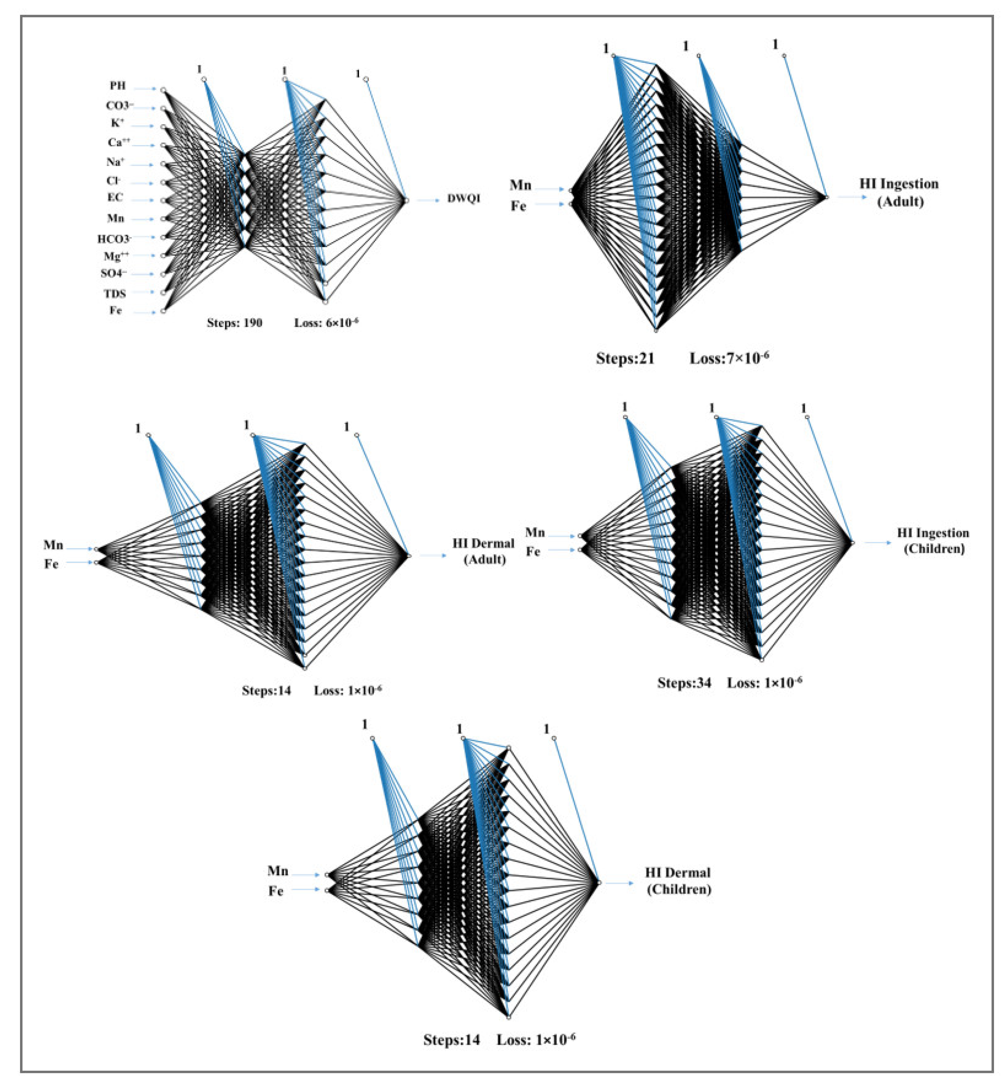
2.5. Back-Propagation Neural Network (BPNN)

One popular type of neural network is the BPNN model, also known as the back-propagation neural network [81]. A neural network model consists of three distinctive layers, which are the input layer, the hidden layer, and the output layer. The input layer is responsible for providing an input to the neural network, while the hidden layer is placed between the independent input layer and the dependent output layer. The hidden layer extracts high-level properties from the input, and the output layer produces outputs based on these inputs. The BPNN model typically has two hidden layers, with the number of nodes determined by the accuracy of the regression. The “activation” nodes, which are often indicated by weight, are found within the hidden layers. The output layer displays the anticipated value of the parameter being measured. Artificial neural network models are generalized mathematical models that are designed to imitate human cognition, specifically with regards to pattern detection and prediction. These models use interconnected nodes or neurons with weighted connections to achieve their objectives [82,83]. The proposed system includes several consecutive phases, which are shown in Figure 3.

The neural network underwent training for a minimum of 1000 iterations, or until the error measurement approached a value of ${10}^{-4}$. To determine the appropriate number of neurons in the hidden layer, a validation process was performed using the leave-one-out cross-validation (LOOCV) method on the training dataset. Due to memory limitations, the Broyden–Fletcher–Goldfarb–Shanno (lbfgs) optimizer was employed as a weight optimizer to enhance the execution speed of the algorithm [84]. The most relevant feature was identified using the algorithm outlined in [47]. This improved the accuracy of the regression model’s future predictions while simultaneously reducing the dimensionality of the data.

Model Evaluation

To assess the effectiveness of a regression model, two commonly used metrics are the coefficient of determination (R²) and the root-mean-square error (RMSE) [85,86]. The parameters being described include “X_act”, which represents the actual value determined by the formula; “X_p”, which is the projected or simulated value; “X_ave”, which is the mean value; and “N”, which refers to the total number of data points.

• Root-mean-square error

$$RMSE=\sqrt{\frac{1}{N}{{\displaystyle \sum }}_{i=1}^N{\left(X_{ act}-X_{ p}\right)}^2}$$

(11)

• Coefficient of determination

$$R^2=\frac{\sum {\left(X_{ act}-X_{ p}\right)}^2}{\sum {\left(X_{ act}-X_{ ave}\right)}^2}$$

(12)

2.6. Software and Datasets Used for Data Analysis

Around 140 samples were utilized during the training and validation phases, with 112 samples (or 80% of the total) used to train and validate the regression model. The remaining 28 cases (or 20%) were used to evaluate the model’s performance by comparing predicted and computed values. The leave-one-out cross-validation approach (LOOCV) was used to train and validate the model, where during each trial, the remaining data were used for training while one sample was omitted for the validation procedure. This technique can reduce overfitting and provide a more accurate estimate of the model’s predictive capability [87]. The Python 3.7.3 programming language, Diagrammes, ArcGIS software, and Excel were utilized for data analysis, model construction, and data preparation. The Scikit-learn package version 0.202 was employed to study the BPNN module for regression tasks. The data were analyzed on a system with an Intel Core i7-3630QM central processing unit operating at 2.4 GHz and 8 GB of RAM.

3. Results and Discussion

3.1. Physicochemical Parameters

The evaluation of GW was carried out based on the physicochemical parameters and its suitability for drinking purposes. These physicochemical parameters were evaluated according to standard limits of the WHO [34] for drinking water (

Table 3. Statistical properties of the investigated physicochemical parameters.

Parameters	Unit	WHO (2017)	Min.	Max.	Mean
Temp.	°C	-	29.0	38.0	33.5
pH	-	8.5	6.10	8.10	6.99
EC	μS/cm	1500	214	2610	931.2
TDS	mg/L	500	203	1870	628.4
K+	mg/L	12	3.50	53.00	25.51
Na+	mg/L	200	4.00	460.0	115.23
Mg2+	mg/L	75	1.45	68.10	21.9
Ca2+	mg/L	50	8.00	180.0	48.14
Cl−	mg/L	250	23.25	620.0	175.53
SO42−	mg/L	250	0.06	575.0	143.47
HCO3−	mg/L	120	10.98	300.0	107.08
CO32−	mg/L	350	0.00	0.00	0.00
Fe	mg/L	0.3	0.12	10.0	2.27
Mn	mg/L	0.1	0.03	0.31	0.15

Note(s): The physicochemical parameters are expressed in units of milligrams per liter (mg/L), while temperature is shown in degrees Celsius (°C) and electrical conductivity (EC) is measured in microsiemens per centimeter (µs/cm).

).

The TDS value ranged from 203 to 1870 mg/L, with a mean value of 628.4 mg/L. It was reported that approximately 38.5% of the samples exceeded the standard limits for drinking. According to Freeze and Cherry [88], the GW ranged from fresh (EC < 1000 μS/cm) to brackish (EC >1000 μS/cm). The pH values of the samples were between 6.1 and 8.1, which revealed the water is alkaline and falls within acceptable limits for drinking water. The calcium concentration range was between 8 mg/L and 180 mg/L, with 71% of the water samples meeting drinking water standards, and only 29% exceeding the limits. All of the samples had an acceptable concentration of Mg²⁺ within drinking water limits, with a maximum value of 68.1 mg/L. Potassium (K⁺) concentrations in 96.5% of the GW samples exceeded the allowable standards for drinking water, with the minimum concentration being 3.50 mg/L and the maximum being 53 mg/L. Approximately 81% of the samples had an acceptable level of sodium (Na⁺) for drinking, with concentrations ranging from 4 mg/L to 460 mg/L. The predominant anions present in the GW were chloride (Cl⁻) and sulfate (SO₄²⁻), with average concentrations of 175.53 mg/L and 143.47 mg/L, respectively. Approximately 21% and 18.5% of the water samples had Cl⁻ and SO₄²⁻ concentrations that exceeded the permissible limits for drinking water, respectively, while the rest were within the standard limits. Approximately 68.5% of the water samples had acceptable bicarbonate (HCO₃⁻) concentrations for drinking water, with an average concentration of 107.08 mg/L. The concentration of iron (Fe) in 97% of the GW samples exceeded the allowable limits for drinking water, with an average concentration of 2.27 mg/L. Moreover, 77% of the GW samples had manganese (Mn) concentrations that were above the permissible limits for drinking water (WHO, 2017 [34]), with an average concentration of 0.15 mg/L. The GW in El Kharga Oasis had high levels of heavy metals, such as Fe and Mn, with an average of concentrations above the limits recommended by the WHO for drinking water.

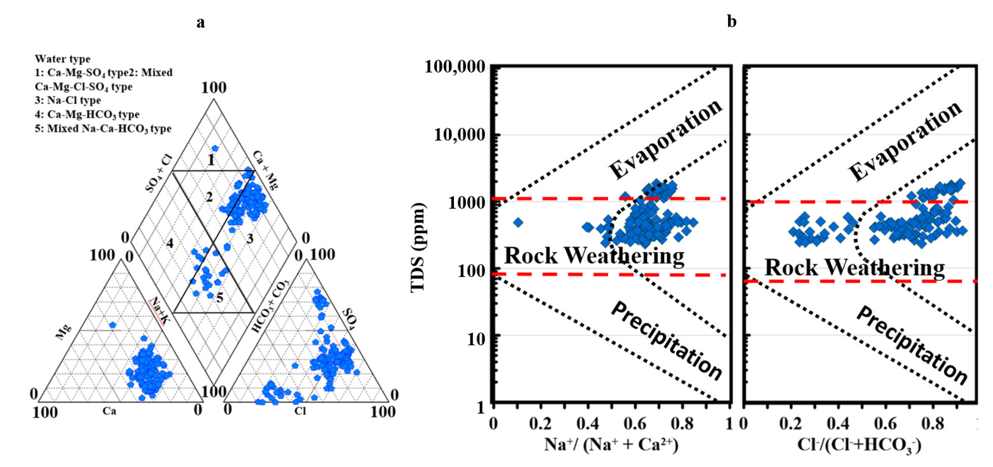
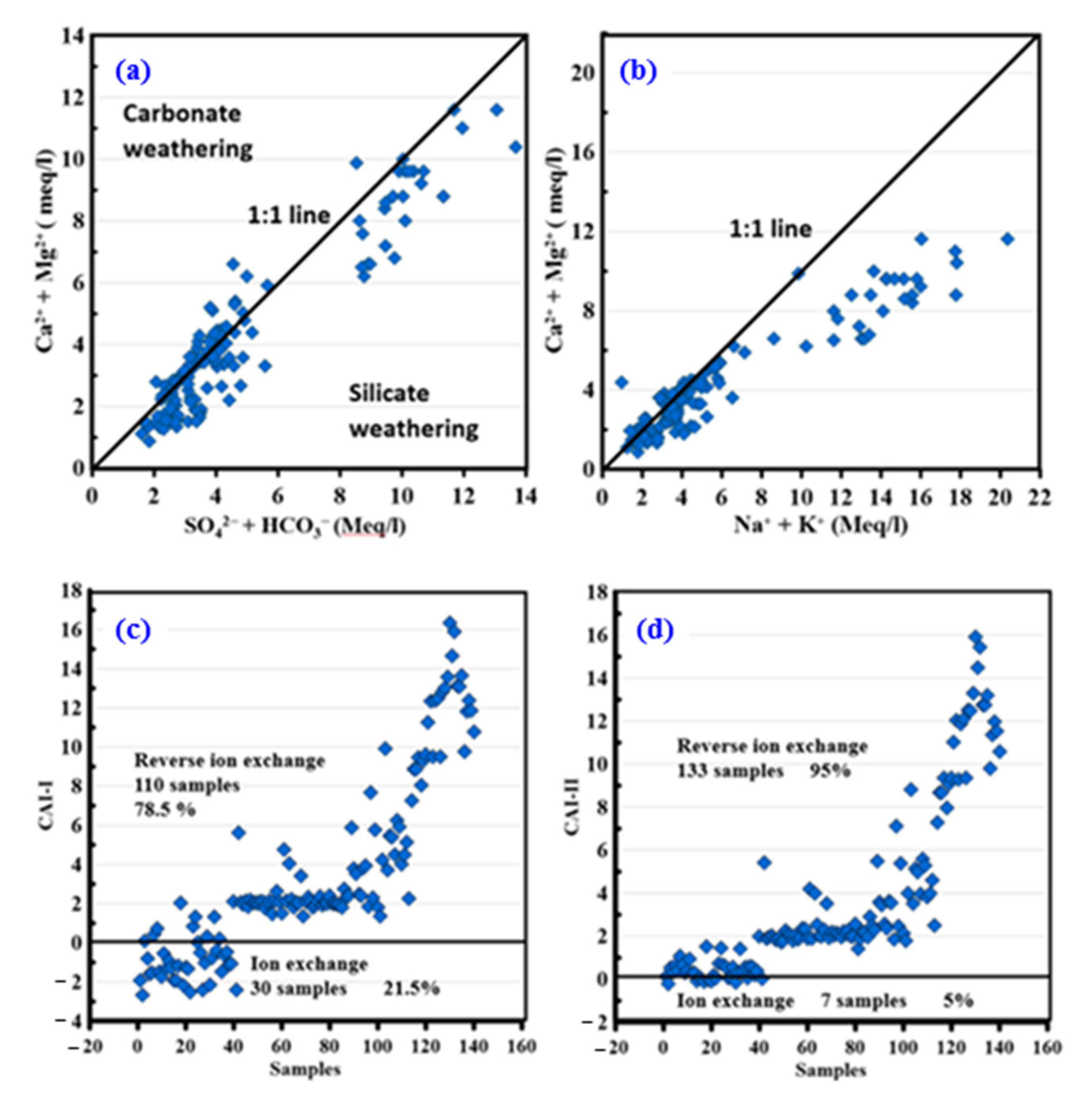
3.2. Geochemical Processes That Control GW Facies

A Piper plot was used to classify the hydrochemical facies of the GW, following the approach outlined in reference [89]. Based on the cationic triangle, 82.14% of the samples were found to be dominant in Na⁺ and K⁺, while 17.14% were not dominant, and the remaining samples were dominated by Mg²⁺. The diamond shape of the Piper plot was used to divide the samples into five distinct hydrochemical facies (as shown in Figure 4a). The Ca–Mg–SO₄ facies zone (Type 1), characterized by permanent hardness, was represented by a single sample. The Na–Cl facies zone (Type 2) was the most dominant, with approximately 88 samples falling within this zone. In addition, there were five samples in the Ca–Mg–HCO₃ facies zone (Type 3) and fifteen samples in the mixed Na–Ca–HCO₃ facies zone (Type 4). The remaining samples were found in the mixed Ca–Mg–Cl–SO₄ zone (Type 5). In nearly all of the samples, the salinity indicators (SO₄²⁻ + Cl⁻) were found to be greater than the alkalinity (HCO³⁻ + CO₃²⁻), and the alkalis (Na⁺ + K⁺) were higher than the alkaline earths (Ca²⁺ + Mg²⁺). These observations suggest that the hydrochemistry of the NSSA region is primarily influenced by these factors. The analysis of the GW samples revealed that the majority of samples fell under the Ca–Mg–HCO₃ and Na–HCO₃ types, indicating the early stages of meteoric water recharge. However, the remaining samples exhibited the Ca–Mg–Cl/SO₄ water type, indicating intermediate stages of water evolution, particularly in the northern and central regions of the study area. The vast majority of the GW samples belonged to the Na–Cl water type, which indicates the final stages of geochemical evolution in the discharge areas, particularly in the southern parts of the study area where the GW flows. These findings corroborated those of earlier studies in the region that utilized geochemical modeling to evaluate the mineral saturation state. A previous study showed that the water was saturated with calcite and dolomite, which means that the water could precipitate these minerals, while the water was undersaturated with halite and gypsum, which refers to the ability of water to dissolve this mineral [10]. The difference in the water type is related to the heterogeneity of the aquifer and different cement materials between gains with wells depth. Several researchers have applied a geochemical model on the NSSA in Egypt, the complex terminal aquifer in Algerian desert, and the Clastic aquifer in the Kuwait region, and found that they contained a hypothetical combination of salts, including NaCl, Na₂SO₄, NaHCO₃, Mg(HCO₃)₂, and Ca(HCO₃)₂, which may have been leached and dissolved from terrestrial salts, perhaps as part of a cation exchange process. Additionally, The GW was undersaturated with regard to halite and gypsum, indicating the ability of water to dissolve these minerals. On the other hand, the GW was oversaturated with calcite, dolomite, iron sulfide, siderite, and silica along its flow paths, indicating a high probability of precipitation of these minerals. Unfortunately, the precipitation of these minerals has negative effects on water quality and public health. The Gibbs [90] diagram is a popular tool for illustrating the interactions between different processes that impact water chemistry. For ease of interpretation, the diagram is divided into three distinct zones (as shown in Figure 4b). The first zone is characterized by low total dissolved solids (TDSs) and high percentages of Cl⁻/(Cl⁻ + HCO₃⁻) and Na+/(Na⁺ + Ca²⁺), indicating the influence of atmospheric precipitation. The second zone had mild TDSs and a cation/anion ratio that indicated rock degradation. The third zone is at the top of the Gibbs plot, with extremely high TDS levels that indicate evaporation and crystallization. According to the scatter plots, 19.28% of the samples fell inside the evaporation/crystallization dominance zone, while the remaining samples were in the rock weathering dominance zone (water–rock interaction). Calcium and bicarbonate ions were the most prevalent in GW samples due to the weathering process in aquifer rocks. The Gibbs diagram data revealed that most samples had brackish TDSs records, indicating that the GW chemical composition in the region is mostly determined by water–rock interactions. The TDSs slightly increased due to evaporation, as seen in the association with both TDSs and Na⁺/(Na⁺ + Ca²⁺).

The main controlling geochemical processes affecting the water chemistry were determined using the ionic ratio and chloro-alkaline index, as depicted in Figure 4. These processes affected the quality of the GW and its suitability for drinking. The relationship between the concentrations of Na⁺ and K⁺ versus Ca²⁺ and Mg²⁺ (Figure 4b) indicates that many of the samples were close to the 1:1 line, suggesting mineral dissolution. Some data points on the graph were located above the line, which suggests that a process of reverse ion exchange has occurred. The prevalence of Na⁺ and K⁺ ions over Ca²⁺ and Mg²⁺ ions in most of the samples indicated that Na⁺ and K⁺ ions had replaced Ca²⁺ and Mg²⁺ ions through ion exchange and silicate weathering. However, a few data points exceeded the 1:1 line, indicating the occurrence of reverse ion exchange. The linear graph in Figure 4a plots the total of Ca²⁺ and Mg²⁺ ions against the total of HCO₃⁻ and SO₄²⁻. This graph shows that the breakdown of gypsum, calcite, and dolomite caused some samples to cross the 1:1 line. The relative increase of SO₄²⁻ and HCO₃⁻ ions compared to Ca²⁺ and Mg²⁺ ions resulted from silicate weathering. Chloro-alkaline indices [91] can be used to interpret the base reaction of ion exchange between the NSSA aquifer material and the GW, and the CAI-I and CAI-II can be computed using specific equations.

CAI−I = [Cl⁻ − (Na⁺ + K⁺)]/ Cl⁻

(13)

CAI−II = [Cl⁻ − (Na⁺ + K⁺)]/(HCO₃⁻ + SO₄²⁻ + NO₃⁻)

(14)

The calculation of CAI-I and CAI-II values can indicate the process that controls the water chemistry (Figure 5c,d). A negative value suggests that the process of ion exchange is the main controlling process, while a positive value indicates that reverse ion exchange is the main controlling process. In this study, most of the water samples (78.5%) had a positive value for CAI-I, and almost all of the samples (95%) had a CAI-II value greater than zero, indicating that reverse ion exchange was the primary process controlling the GW chemistry in NSSA. These results suggest that calcium and magnesium in the rocks or sediments of the NSSA aquifer replaced sodium and potassium in the GW. Only a small percentage of water samples (21.5% for CAI-I and 5% for CAI-II) had negative values.

1/2Ca²⁺-X + Na⁺ → 1/2Ca²⁺ + Na⁺-X reverse ion exchange

(15)

Na⁺-X + 1/2Ca²⁺ → Na⁺ + 1/2Ca²⁺-X ion exchange

(16)

3.3. Statistical Analysis

3.3.1. Cluster Analysis

A combination of the Wards’ linkage approach and Euclidean distance was used to determine how similar the GW samples were. The dendrogram shown in Figure 6 was used to categorize the various physicochemical factors in the acquired GW samples. For statistical reasons, standard scores (Z-scores) were produced for each variable and applied [92]. All variables were log-transformed and nearly matched the normal distribution. Three primary groups were identified in the dendrogram of the ten physicochemical parameters (HCO₃⁻, SO₄²⁻, Cl⁻, Mg²⁺, Ca²⁺, K⁺, Na⁺, Fe, Mn, and TDS) (Figure 6).

The R-mode cluster analysis executed on the GW samples produced three clusters (Figure 6a). At a connection distance of ten (10) physicochemical parameters, the hydrochemical characteristics of the groups could be separated at this distance [93], which is represented in Figure 5 with a red color. According to the results, height variables were divided into two clusters that were managed by the TDSs (Figure 6). The groups are as follows: There were Na⁺, SO₄²⁻, and Cl⁻ evaporite components in G1. G2 contained practically all carbonate components and the metals Ca²⁺, Mg²⁺, K⁺, Fe, Mn, and HCO₃⁻. TDSs (G3) had two separate sources, the first of which was evaporitic, and the second of which was carbonate. G1 showed a strong correlation between evaporate characteristics, such as SO₄²⁻ and Cl⁻, showing that chlorides and salts were primarily responsible for this GW’s salinity in the research region. However, the substantial dominance of Mg²⁺ and Ca²⁺ in the chemical makeup of our GW, such as sulfates or anhydrite, and the calcium of sulfates led to the G2 revealing a strong link between the carbonate’s characteristics [38]. Both G1 and G2 showed that the aquifer’s waters in this study area were primarily mineralized due to the lithological component. Finally, G3 demonstrated that all metrics had varied associations with this region’s salinity, which had grown. The Q-mode cluster analysis performed on 140 sampling locations retained three clusters (Figure 6b). Cluster 1 comprised 27 sampling sites, which were S114–S140. Cluster 2 comprised 56 sampling sites, which were S1–S3, S8, S9, S12–S38, S43, S45–S50, S54, S55, S57, S58, S60, S62, S63, S66, S69, S71, S74–S82, S88, and S105. Cluster 3 comprised 57 sampling sites, which were S4–S7, S10, S11, S27, S32, S39–S42, S44, S51–S53, S56, S59, S61, S64, S65, S67, S68, S70, S72, S73, S77, S80, S87, S89, and S90–S113. The close similarity of the water quality characteristics of the sample stations in Clusters 1 and 2 was indicated by the small Euclidean distance between them. Clusters 1 and 2 had greater Euclidean distances than Cluster 3, which indicated that the water quality within these clusters was highly variable. Domestic influences may be shown at sites in Cluster 2, whereas sites in Cluster 1 showed the impact of GW contamination from fertilizer leaching. However, due to overexploitation, Cluster 3 sites exhibited saltwater intrusion, which emphasizes the impact of solubilization in the aquifer.

3.3.2. Principal Component Analysis (PCA)

The correlation matrix and Bartlett’s test of sphericity were used to determine if the data could be used for PCA.

Table 4. Correlation of the various parameters and factors.

Parameter	Factor 1	Factor 2	Factor 3	Factor 4
TDS	−0.967	−0.071	−0.030	0.042
K+	0.756	−0.335	−0.155	−0.107
Na+	−0.981	−0.022	0.007	0.073
Mg2+	−0.744	0.282	−0.126	−0.033
Ca2+	−0.962	−0.017	−0.016	0.038
Cl−	−0.980	0.022	−0.075	0.069
SO42−	−0.929	−0.070	−0.251	0.127
HCO3−	−0.432	0.151	0.814	−0.321
Fe	0.433	0.372	0.246	0.768
Mn	0.259	0.835	−0.299	−0.300

shows the Kaiser–Meyer–Olkin (KMO) measure of sampling adequacy. The KMO value (0.649) obtained was greater than 0.5 and Bartlett’s test of sphericity value (0.000) was less than 0.05. The KMO and Bartlett’s tests are measures of how appropriate data are for factor analysis, which measures sampling suitability for each individual variable in the model. Retained items had correlation coefficients of above 0.3. Any correlation coefficients of less than 0.3 and Bartlett’s test values above 0.05 were not used, as suggested by Mustapha et al. [94].

Four of the original components were kept after the PCA (F1, F2, F3 and F4). F1 accounted for 62.18 percent of the data set’s variability, whereas F2, F3, and F4 accounted for 10.63, 9.24, and 8.26% of it, respectively (Figure 7). In Table 4, the variables’ loading values are shown. There was a strong connection between the factors and the variables, as indicated by the value being near to 1. According to [95], these loads were further divided into three categories: high (>0.75), moderate (from 0.75 to 0.50), and weak (from 0.50 to 0.30). F1 showed that strong negative relationships exist between Mg²⁺, Ca²⁺, Na⁺, K⁺, Cl⁻, SO₄²⁻, and TDS, which illustrated that the source of salinity was from the weathering of limestone, dissolution of pyrite, halite, and gypsum, and multiple ion exchange processes in the water system [96]. Therefore, the factor can be termed a salinization factor. SO₄²⁻ can be produced by the oxidation of Sulphur compounds or by fertilizer. However, anthropogenic causes, including irrigation water quality, household waste, and uncontrolled fertilization, may be to blame for the Ca²⁺, Na⁺, and Mg²⁺. Additionally, the development of salts and soil weathering may be the cause of the chloride. A strong positive association between F2 and Mn (+0.835), and between F4 and Fe (+0.768), indicated that alkaline water was moving through the rocks and soil. These findings illuminated the process through which human behaviors take place. Factor 3 had substantial positive loadings in HCO₃⁻, which are +0.814 (Table 4). This information suggests that the element did not have any impact on the overall mineral content of water. It also predicts that the formation of HCO₃₋ occurs as a result of the weathering of carbonates, and indicates that the chemistry of GW may be affected by acid–base equilibrium conditions [97].

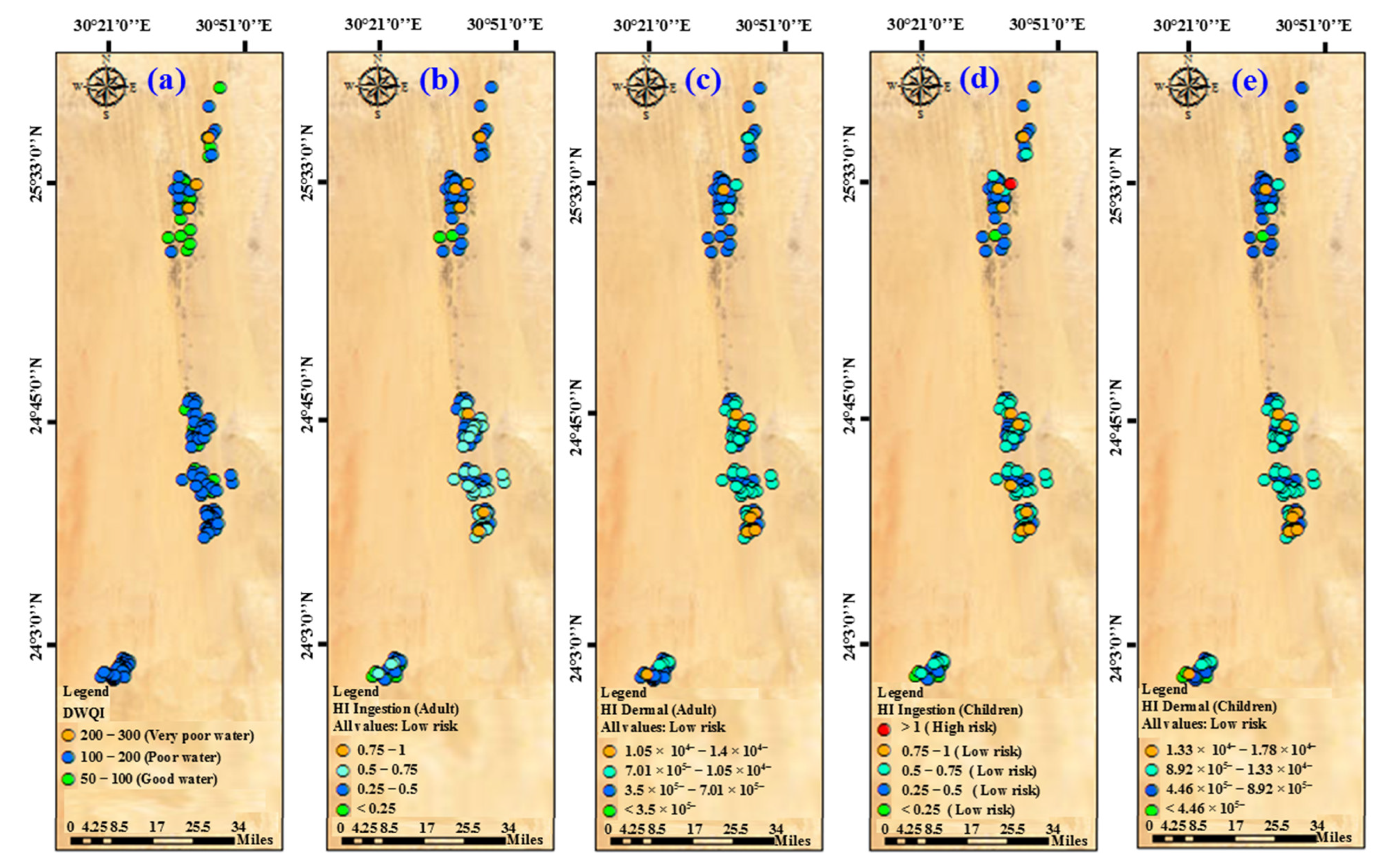
3.4. Water Quality Indices (WQIs)

Table 5. Statistical analysis and classes of water quality indices.

	Indices	Min	Max	Mean	Range	Class	No. of Samples (%)
					<50	Excellent water	0.0 (0.0%)
					50–100	Good water	37 (26.4%)
	DWQI	55.06	239.03	121.19	100–200	Poor water	100(71.5%)
					200–300	Very poor water	3.0 (2.1%)
					>300	Unsuitable	0.0 (0.0%)
Children	HI (ingestion)	0.084	1.045	0.467	<1	Low risk	139 (99.2%) 1.0 (0.8%)
					>1	High risk
	HI (dermal)	1.72 × 10−5	1.78 × 10−4	8.74 × 10−5	<1	Low risk	140 (100%) 0.0 (0.0%)
					>1	High risk
Adult	HI (ingestion)	0.08	0.97	0.43	<1	Low risk	140 (100%) 0.0 (0.0%)
					>1	High risk
	HI (dermal)	1.4 × 10−5	1.4 × 10−4	6.9 × 10−5	<1	Low risk	140 (100%) 0.0 (0.0%)
					>1	High risk

provides statistical information on various WQIs, such as the DWQI, HI (ingestion), and HI (dermal). The range of DWQI values was from 55.06 to 239.03, with an average value of 121.19. The results showed that 26.4% of GW samples were classified as good-quality water (northern and central parts of El Kharga Oasis), while 71.5% fell into the poor-quality water category (from north to south of El Kharga Oasis), and 2.1% were categorized as very poor-quality water for drinking (in the northern part of El Kharga Oasis). The spatial distribution map of the DWQI indicated that most of the degradation in GW quality was observed in three locations in the northern part of the study area (Figure 8a). Even though drinkable GW was found in certain areas of the northern and central parts of the study location, the majority of the samples highlighted that water treatment was necessary for the entire area, particularly in the southern portion.

3.5. Assessing Health Risk

The potential health risks associated with exposure to heavy metals for both adults and children were evaluated using the chronic daily intake (CDI), hazard quotient (HQ), and hazard index (HI). CDI measures the daily exposure of humans to metal contaminants in mg L⁻¹ day⁻¹, while HQ assesses the potential risk to human health from heavy metal exposure, with values greater than one (>1) considered harmful. Similarly, HI evaluates the risk posed by various heavy metals.

Table 6. Statistical description of the CDI and HQ for Fe and Mn in adults and children.

Parameters	Type	Min	Max	Mean
CDI ingestion (Fe)	Child	0.006	0.499	0.113
	Adult	0.006	0.46	0.105
CDI ingestion (Mn)	Child	0.001	0.015	0.007
	Adult	0.001	0.014	0.007
CDI dermal (Fe)	Child	6.2 × 10−8	5.1 × 10−6	1.2 × 10−6
	Adult	4.9 × 10−8	4 × 10−6	9.2 × 10−7
CDI dermal (Mn)	Child	1.5 × 10−8	1.6 × 10−7	7.6 × 10−8
	Adult	1.2 × 10−8	1.3 × 10−7	6 × 10−8
HQ ingestion (Fe)	Child	0.009	0.712	0.162
	Adult	0.008	0.659	0.147
HQ ingestion (Mn)	Child	0.06	0.64	0.31
	Adult	0.06	0.6	0.28
HQ dermal (Fe)	Child	4.4 × 10−7	3.7 × 10−5	8.3 × 10−6
	Adult	3.5 × 10−7	2.9 × 10−5	6.6 × 10−6
HQ dermal (Mn)	Child	1.6 × 10−5	1.7 × 10−4	7.9 × 10−5
	Adult	1.3 × 10−5	1.3 × 10−4	6.2 × 10−5

provides a summary of the CDI and HQ values observed for the two groups. The CDI ingestion values for Fe and Mn were within the limits (<1) and do not currently pose a serious threat to human health. However, the CDI Ingestion values for Fe were higher than those for Mn, with average values of 0.105 mg L⁻¹ day⁻¹ and 0.113 mg L⁻¹ day⁻¹ for adults and children, respectively. The CDI dermal values were also less than one for both groups. The HQ ingestion and HQ dermal values showed a similar trend to CDI, with higher ingestion values than dermal. The mean HQ ingestion values for Fe and Mn were less than one for both adults and children, but Mn had the highest mean HQ ingestion values for both groups (0.31 for children and 0.28 for adults). The maximum HQ ingestion values for Fe were 0.659 and 0.712 for adults and children, respectively. HQ dermal values were also higher for children compared to adults, as presented in Table 6.

Figure 8b–e depict the calculated water quality indices, HI ingestion and HI dermal values for both adults and children. For adults, the mean value of HI ingestion was 0.43, ranging from 0.08 to 0.97, while for children the mean value was higher, ranging from 0.084 to 1.045. The outcomes revealed that heavy metal contamination through the consumption of GW posed a low human health risk, with 99.2% of samples exhibiting HI ingestion values below 1. Nonetheless, one sample had a HI Ingestion value exceeding 1, indicating high-risk exposure to heavy metals, which could harm children’s health since they consume more water per unit of body weight than adults. Children may be more sensitive to certain contaminants than adults. For example, their developing bodies may be more susceptible to the effects of certain chemicals or toxins such as Fe and Mn. The contaminants could be from natural sources, such as minerals leaching from rocks and soil, or from human activities, such as agricultural or industrial practices. The HI dermal values for all samples in the study area were within permissible limits, and they all fell into the low-risk category. However, the mean value for children (8.74 × 10⁻⁵) was greater than that for adults (6.9 × 10⁻⁵). Treatment is recommended for areas with a high health risk to protect children’s health.

3.6. The Performance of ANN to Predict Drinking Water Quality and Health Risk

Table 7. Performance criteria of the simulation models for Drinking Water Quality and Health Risk.

		Parameters	Training		Cross-Validation		Test
Variable	Ranking *	(h1, h2, fn)	R2	RMSE	R2	RMSE	R2	RMSE
DWQI	pH, CO32−, K+, Ca2+, Na+, Cl−, EC, Mn, HCO3−, Mg2+, SO42−, TDS, Fe	(6, 12, relu)	0.999 ***	0.00024	0.999	0.00018	0.999 ***	0.00044
HI ingestion (adult)	Mn, Fe	(21, 9, identity)	1.000 ***	4.031 × 10−7	1.0	1.609 × 10−7	1.000 ***	3.995 × 10−7
HI dermal (adult)	Mn, Fe	(9, 18, identity)	0.999 ***	1.859 × 10−6	0.999	2.233 × 10−6	0.999 ***	1.641 × 10−6
HI ingestion (children)	Mn, Fe	(12, 18, identity)	1.000 ***	2.406 × 10−7	1.0	1.413 × 10−7	1.000 ***	1.259 × 10−7
HI dermal (children)	Mn, Fe	(9, 18, identity)	0.999 ***	1.777 × 10−6	0.999	1.601 × 10−6	0.999 ***	1.584 × 10−6

Note(s): h₁ and h₂ are the number of neurons in the two hidden layers, fn is the activation function, and * indicates the most important variables in ascending order. ***, significant at p ≤ 0.001 level.

presents the amalgamation of analyzed characteristics (AC), optimal parameters, and the outputs of the ANN model concerning the RMSE and R² for the training, cross-validation (CV), and test data sets. These elements received high marks for measuring the criteria under consideration. Training the neural network using the super elements’ characteristics (independent variables) allowed for accurate prediction of the investigated parameters (dependent variable). Based on its results, ANN-SC-13 was the most accurate prediction model, since it demonstrated the strongest correlation between the best characteristics and the DWQI. This model’s thirteen characteristics were extremely important for predicting DWQI.

Its value of R² was 0.99 for the training, CV, and test data. The ANN-SC-2 model was the best for measuring HI ingestion in adults. The R² values for the training, CV, and test data were 1, 1, and 1, respectively. The ANN-SC-2 model was the most accurate at detecting HI dermal in adults (R² = 0.99, 0.99, and 0.99 for the training, CV, and test data sets, respectively). The ANN-SC-2 model outperformed the others in predicting HI ingestion in children. This model increased the R² value to 100% for the training, CV, and test data sets. For projecting HI dermal for children, the ANN-SC-2 model exceeded expectations. The value of R² was 0.99 for the training, CV, and test data sets. Elsherbiny et al. [98] reported that the performance of the regression model was enhanced by implementing a series of steps during the training process, including the filtration of high-level features and the tuning of model hyperparameters, to ensure robust prediction. After obtaining senior study features, the optimal neural network topology was determined and is presented in Figure 9. This diagram illustrates the network designs that were chosen for the model.

4. Conclusions

This research assessed GW quality using a combination of physicochemical parameters and WQIs, supported with multivariate analysis, ANN models, and GIS tools to categorize the GW of the NSSA of El Kharga Oasis into distinct hydrogeochemical classes, with a particular focus on its suitability for drinking and the health risk it posed. Through analysis of the collected physicochemical data, various hydrochemical facies of GW were identified, including Ca–Mg–SO₄, mixed Ca–Mg–Cl–SO₄, Na–Cl, Ca–Mg–HCO₃, and mixed Na–Ca–HCO₃ types. These facies were found to be a result of silicate weathering; the dissolution of gypsum, calcite, and dolomite; halite; rock–water interactions; and reverse ion exchange processes. The DWQI results showed that GW samples could be classified for drinking purposes into various levels. The DWQI categorized most of the samples as not suitable for drinking (poor to very poor class), while some samples fell in the good water class. The GW in El Kharga Oasis had high levels of heavy metals, particularly iron and manganese. The average concentrations of these heavy metals were above the limits recommended by the WHO for drinking water. The results of HI analysis indicated a potential health risk due to ingesting GW, with the risk being higher for children in only one location. However, for both children and adults, there was a low risk of dermal and ingestion exposure to the water in all locations.

The ANN models showed good performance in predicting the DWQI and HI with reasonable accuracy. The ANN-SC-2 model outperformed the others in predicting HI ingestion in children. This model increased the R² value to 100% for the training, CV, and test data sets. For projecting HI dermal for children, the ANN-SC-2 model exceeded expectations. The value of R² was 0.99 for the training, CV, and test data sets. The evaluation and prediction of GW quality are very important for managing GW resources. Thus, the WQIs approach integrated with ANN models was introduced to estimate and forecast the GW quality in the NSSA. Therefore, the implemented approach model structure in this context accurately estimated the GW quality using physicochemical variables with relatively minor errors and proved a quite robust performance.

References

1. Liu, J.; Gao, M.; Jin, D.; Wang, T.; Yang, J. Assessment of Groundwater Quality and Human Health Risk in the Aeolian-Sand Area of Yulin City, Northwest China. Expo. Health 2020, 12, 671–680. [Google Scholar] [CrossRef]
2. Snousy, M.G.; Wu, J.; Su, F.; Abdelhalim, A.; Ismail, E. Groundwater Quality and Its Regulating Geochemical Processes in Assiut Province, Egypt. Expo. Health 2022, 14, 305–323. [Google Scholar] [CrossRef]
3. Li, P. To Make the Water Safer. Expo. Health 2020, 12, 337–342. [Google Scholar] [CrossRef] [PubMed]
4. Salameh, M.T.B.; Alraggad, M.; Harahsheh, S.T. The Water Crisis and the Conflict in the Middle East. Sustain. Water Resour. Manag. 2021, 7, 69. [Google Scholar] [CrossRef]
5. Wang, Z.-Y.; Qiu, J.; Li, F.-F. Hybrid Models Combining EMD/EEMD and ARIMA for Long-Term Streamflow Forecasting. Water 2018, 10, 853. [Google Scholar] [CrossRef] [Green Version]
6. Liu, J.; Han, G. Distributions and Source Identification of the Major Ions in Zhujiang River, Southwest China: Examining the Relationships Between Human Perturbations, Chemical Weathering, Water Quality and Health Risk. Expo. Health 2020, 12, 849–862. [Google Scholar] [CrossRef]
7. Keesari, T.; Roy, A.; Pant, D.; Sinha, U.K.; Kumar, P.V.N.; Rao, L.V. Major Ion, Trace Metal and Environmental Isotope Characterization of Groundwater in Selected Parts of Uddanam Coastal Region, Andhra Pradesh, India. J. Earth Syst. Sci. 2020, 129, 205. [Google Scholar] [CrossRef]
8. Katla, S.; Gugulothu, S.; Dhakate, R. Spatial Assessment of Major Ion Geochemistry in the Groundwater around Suryapet Region, Southern Telangana, India. Environ. Sustain. 2021, 4, 107–122. [Google Scholar] [CrossRef]
9. Arafa, N.A.; Salem, Z.E.-S.; Ghorab, M.A.; Soliman, S.A.; Abdeldayem, A.L.; Moustafa, Y.M.; Ghazala, H.H. Evaluation of Groundwater Sensitivity to Pollution Using GIS-Based Modified DRASTIC-LU Model for Sustainable Development in the Nile Delta Region. Sustainability 2022, 14, 14699. [Google Scholar] [CrossRef]
10. Gad, M.; Dahab, K.; Ibrahim, H. Applying of a Geochemical Model on the Nubian Sandstone Aquifer in Siwa Oasis, Western Desert, Egypt. Environ. Earth Sci. 2018, 77, 401. [Google Scholar] [CrossRef]
11. Eid, M.H.; Elbagory, M.; Tamma, A.A.; Gad, M.; Elsayed, S.; Hussein, H.; Moghanm, F.S.; Omara, A.E.-D.; Kovács, A.; Péter, S. Evaluation of Groundwater Quality for Irrigation in Deep Aquifers Using Multiple Graphical and Indexing Approaches Supported with Machine Learning Models and GIS Techniques, Souf Valley, Algeria. Water 2023, 15, 182. [Google Scholar] [CrossRef]
12. Gaagai, A.; Aouissi, H.A.; Bencedira, S.; Hinge, G.; Athamena, A.; Haddam, S.; Gad, M.; Elsherbiny, O.; Elsayed, S.; Eid, M.H.; et al. Application of Water Quality Indices, Machine Learning Approaches, and GIS to Identify Groundwater Quality for Irrigation Purposes: A Case Study of Sahara Aquifer, Doucen Plain, Algeria. Water 2023, 15, 289. [Google Scholar] [CrossRef]
13. Gad, M.; El Osta, M. Geochemical Controlling Mechanisms and Quality of the Groundwater Resources in El Fayoum Depression, Egypt. Arab. J. Geosci. 2020, 13, 861. [Google Scholar] [CrossRef]
14. Ibrahim, H.; Yaseen, Z.M.; Scholz, M.; Ali, M.; Gad, M.; Elsayed, S.; Khadr, M.; Hussein, H.; Ibrahim, H.H.; Eid, M.H.; et al. Evaluation and Prediction of Groundwater Quality for Irrigation Using an Integrated Water Quality Indices, Machine Learning Models and GIS Approaches: A Representative Case Study. Water 2023, 15, 694. [Google Scholar] [CrossRef]
15. Mester, T.; Szabó, G.; Bessenyei, É.; Karancsi, G.; Barkóczi, N.; Balla, D. The Effects of Uninsulated Sewage Tanks on Groundwater. A Case Study in an Eastern Hungarian Settlement. J. Water Land Dev. 2017, 33, 123–129. [Google Scholar] [CrossRef] [Green Version]
16. Abdel-Galil, F.A.; Amro, M.A.; Abdel-Moniem, A.S.H.; El-Fandary, O.O. Population Fluctuations and Interspecific Competition between Tephritid Flies Attacking Fruit Crops in the New Valley Oases, Egypt. Arch. Phytopathol. Plant Prot. 2010, 43, 647–659. [Google Scholar] [CrossRef]
17. Balat, E.G. Environmental Assessment Report for New Valley Governorate El Mounira and Naser El Thowra Villages, Kharga Oasis. 2007. Environmental Assessment Report. National Organization for Potable Water and Sanitary Drainage (NOPWASD). Available online: https://pdf.usaid.gov/pdf_docs/Pnadj893.pdf (accessed on 7 March 2023).
18. El Osta, M.; Hussein, H.; Tomas, K. Numerical Simulation of Groundwater Flow and Vulnerability in Wadi El-Natrun Depression and Vicinities, West Nile Delta, Egypt. J. Geol. Soc. India 2018, 92, 235–247. [Google Scholar] [CrossRef]
19. Hassan, I.; Elhassan, B. Heavy Metals Pollution and Trend in the River Nile System. Am. Sci. Res. J. Eng. Technol. Sci. 2016, 21, 69–76. [Google Scholar]
20. Peng, H.; Yang, W.; Nadine Ferrer, A.S.; Xiong, S.; Li, X.; Niu, G.; Lu, T. Hydrochemical Characteristics and Health Risk Assessment of Groundwater in Karst Areas of Southwest China: A Case Study of Bama, Guangxi. J. Clean. Prod. 2022, 341, 130872. [Google Scholar] [CrossRef]
21. Jabbo, J.N.; Isa, N.M.; Aris, A.Z.; Ramli, M.F.; Abubakar, M.B. Geochemometric Approach to Groundwater Quality and Health Risk Assessment of Heavy Metals of Yankari Game Reserve and Its Environs, Northeast Nigeria. J. Clean. Prod. 2022, 330, 129916. [Google Scholar] [CrossRef]
22. Mackay, D.M.; Cherry, J.A. Groundwater Contamination: Pump-and-Treat Remediation. Environ. Sci. Technol. 1989, 23, 630–636. [Google Scholar] [CrossRef]
23. Medici, G.; West, L.J. Review of Groundwater Flow and Contaminant Transport Modelling Approaches for the Sherwood Sandstone Aquifer, UK; Insights from Analogous Successions Worldwide. Q. J. Eng. Geol. Hydrogeol. 2022, 55, qjegh2021-176. [Google Scholar] [CrossRef]
24. Gad, M.; El-Hattab, M. Integration of Water Pollution Indices and DRASTIC Model for Assessment of Groundwater Quality in El Fayoum Depression, Western Desert, Egypt. J. Afr. Earth Sci. 2019, 158, 103554. [Google Scholar] [CrossRef]
25. Gad, M.; Dahab, K.; Ibrahim, H. Impact of Iron Concentration as a Result of Groundwater Exploitation on the Nubian Sandstone Aquifer in El Kharga Oasis, Western Desert, Egypt. NRIAG J. Astron. Geophys. 2016, 5, 216–237. [Google Scholar] [CrossRef] [Green Version]
26. Singh, R.; Sao, S. Evaluation of Water Quality by Physicochemical Parameters, Heavy Metal and Use of Metal Resistant Property of Bacteria for Bioremediation of Heavy Metals. World J. Environ. Pollut. 2015, 5, 23–28. [Google Scholar]
27. Alqarawy, A.; El Osta, M.; Masoud, M.; Elsayed, S.; Gad, M. Use of Hyperspectral Reflectance and Water Quality Indices to Assess Groundwater Quality for Drinking in Arid Regions, Saudi Arabia. Water 2022, 14, 2311. [Google Scholar] [CrossRef]
28. El Osta, M.; Masoud, M.; Alqarawy, A.; Elsayed, S.; Gad, M. Groundwater Suitability for Drinking and Irrigation Using Water Quality Indices and Multivariate Modeling in Makkah Al-Mukarramah Province, Saudi Arabia. Water 2022, 14, 483. [Google Scholar] [CrossRef]
29. Cieszynska, M.; Wesolowski, M.; Bartoszewicz, M.; Michalska, M.; Nowacki, J. Application of Physicochemical Data for Water-Quality Assessment of Watercourses in the Gdansk Municipality (South Baltic Coast). Environ. Monit. Assess. 2012, 184, 2017–2029. [Google Scholar] [CrossRef] [Green Version]
30. Farid, S.; Baloch, M.K.; Ahmad, S.A. Water Pollution: Major Issue in Urban Areas. Int. J. Water Resour. Environ. Eng. 2012, 4, 55–65. [Google Scholar]
31. Sadashivaiah, C.; Ramakrishnaiah, C.; Ranganna, G. Hydrochemical Analysis and Evaluation of Groundwater Quality in Tumkur Taluk, Karnataka State, India. Int. J. Environ. Res. Public Health 2008, 5, 158–164. [Google Scholar] [CrossRef]
32. Khadr, M.; Gad, M.; El-Hendawy, S.; Al-Suhaibani, N.; Dewir, Y.H.; Tahir, M.U.; Mubushar, M.; Elsayed, S. The Integration of Multivariate Statistical Approaches, Hyperspectral Reflectance, and Data-Driven Modeling for Assessing the Quality and Suitability of Groundwater for Irrigation. Water 2020, 13, 35. [Google Scholar] [CrossRef]
33. Batarseh, M.; Imreizeeq, E.; Tilev, S.; Al Alaween, M.; Suleiman, W.; Al Remeithi, A.M.; Al Tamimi, M.K.; Al Alawneh, M. Assessment of Groundwater Quality for Irrigation in the Arid Regions Using Irrigation Water Quality Index (IWQI) and GIS-Zoning Maps: Case Study from Abu Dhabi Emirate, UAE. Groundw. Sustain. Dev. 2021, 14, 100611. [Google Scholar] [CrossRef]
34. WHO. Guidelines for Drinking-Water Quality; World Health Organization: Geneva, Switzerland, 2004; Volume 1, ISBN 92-4-154638-7. [Google Scholar]
35. Wasserman, G.A.; Liu, X.; Parvez, F.; Ahsan, H.; Levy, D.; Factor-Litvak, P.; Kline, J.; van Geen, A.; Slavkovich, V.; LoIacono, N.J.; et al. Water Manganese Exposure and Children’s Intellectual Function in Araihazar, Bangladesh. Environ. Health Perspect. 2006, 114, 124–129. [Google Scholar] [CrossRef] [Green Version]
36. Kell, D.B. Towards a Unifying, Systems Biology Understanding of Large-Scale Cellular Death and Destruction Caused by Poorly Liganded Iron: Parkinson’s, Huntington’s, Alzheimer’s, Prions, Bactericides, Chemical Toxicology and Others as Examples. Arch. Toxicol. 2010, 84, 825–889. [Google Scholar] [CrossRef] [Green Version]
37. Powers, K.M.; Smith-Weller, T.; Franklin, G.M.; Longstreth, W.T.; Swanson, P.D.; Checkoway, H. Parkinson’s Disease Risks Associated with Dietary Iron, Manganese, and Other Nutrient Intakes. Neurology 2003, 60, 1761–1766. [Google Scholar] [CrossRef]
38. Abuzaid, A.S.; Jahin, H.S. Combinations of multivariate statistical analysis and analytical hierarchical process for indexing surface water quality under arid conditions. J. Contam. Hydrol. 2022, 248, 104005. [Google Scholar] [CrossRef]
39. Athamena, A.; Gaagai, A.; Aouissi, H.A.; Burlakovs, J.; Bencedira, S.; Zekker, I.; Krauklis, A.E. Chemometrics of the Environment: Hydrochemical Characterization of Groundwater in Lioua Plain (North Africa) Using Time Series and Multivariate Statistical Analysis. Sustainability 2023, 15, 20. [Google Scholar] [CrossRef]
40. Roubil, A.; El Ouali, A.; Bülbül, A.; Lahrach, A.; Mudry, J.; Mamouch, Y.; Essahlaoui, A.; El Hmaidi, A.; El Ouali, A. Groundwater Hydrochemical and Isotopic Evolution from High Atlas Jurassic Limestones to Errachidia Cretaceous Basin (Southeastern Morocco). Water 2022, 14, 1747. [Google Scholar] [CrossRef]
41. Gaagai, A.; Boudoukha, A.; Boumezbeur, A.; Benaabidate, L. Hydrochemical Characterization of Surface Water in the Babar Watershed (Algeria) Using Environmetric Techniques and Time Series Analysis. Int. J. River Basin Manag. 2017, 15, 361–372. [Google Scholar] [CrossRef]
42. Beltran, N.H.; Duarte-Mermoud, M.A.; Soto Vicencio, V.A.; Salah, S.A.; Bustos, M.A. Chilean Wine Classification Using Volatile Organic Compounds Data Obtained with a Fast GC Analyzer. IEEE Trans. Instrum. Meas. 2008, 57, 2421–2436. [Google Scholar] [CrossRef] [Green Version]
43. Guyon, I.; Elisseeff, A. An Introduction to Variable and Feature Selection. J. Mach. Learn. Res. 2003, 3, 1157–1182. [Google Scholar]
44. Schulze, F.H.; Wolf, H.; Jansen, H.W.; van der Veer, P. Applications of Artificial Neural Networks in Integrated Water Management: Fiction or Future? Water Sci. Technol. 2005, 52, 21–31. [Google Scholar] [CrossRef] [PubMed]
45. ElMasry, G.; Sun, D.-W.; Allen, P. Near-Infrared Hyperspectral Imaging for Predicting Colour, PH and Tenderness of Fresh Beef. J. Food Eng. 2012, 110, 127–140. [Google Scholar] [CrossRef]
46. Strobl, C.; Boulesteix, A.-L.; Kneib, T.; Augustin, T.; Zeileis, A. Conditional Variable Importance for Random Forests. BMC Bioinform. 2008, 9, 307. [Google Scholar] [CrossRef] [Green Version]
47. Glorfeld, L. A Methodology for Simplification and Interpretation of Backpropagation-Based Neural Network Models. Expert Syst. Appl. 1996, 10, 37–54. [Google Scholar] [CrossRef]
48. Melis, G.; Dyer, C.; Blunsom, P. On the State of the Art of Evaluation in Neural Language Models. arXiv 2017. [Google Scholar] [CrossRef]
49. Bergstra, J.; Yamins, D.; Cox, D. Making a Science of Model Search: Hyperparameter Optimization in Hundreds of Dimensions for Vision Architectures. In Proceedings of the 30th International Conference on Machine Learning, Atlanta, GA, USA, 16–21 June 2013; Dasgupta, S., McAllester, D., Eds.; PMLR: Proceedings of Machine Learning Research. Volume 28, pp. 115–123. [Google Scholar]
50. Wu, J.; Chen, X.-Y.; Zhang, H.; Xiong, L.-D.; Lei, H.; Deng, S.-H. Hyperparameter Optimization for Machine Learning Models Based on Bayesian Optimization. J. Electron. Sci. Technol. 2019, 17, 26–40. [Google Scholar]
51. Assaad, F.A. Hydrogeological Aspects and Environmental Concerns of the New Valley Project, Western Desert, Egypt, with Special Emphasis on the Southern Area. Environ. Geol. Water Sci. 1988, 12, 141–161. [Google Scholar] [CrossRef]
52. Kehl, H.; Bornkamm, R. Landscape Ecology and Vegetation Units of the Western Desert of Egypt. Catena. Suppl. 1993, Num. 26, pp. 155–178; Illustration; ref. 84 ref. ISSN 0722-0723. Available online: https://pascal-francis.inist.fr/vibad/index.php?action=getRecordDetail&idt=6318102 (accessed on 7 March 2023).
53. Salman, A.B.; Howari, F.M.; El-Sankary, M.M.; Wali, A.M.; Saleh, M.M. Environmental Impact and Natural Hazards on Kharga Oasis Monumental Sites, Western Desert of Egypt. J. Afr. Earth Sci. 2010, 58, 341–353. [Google Scholar] [CrossRef]
54. Lamoreaux, P.E.; Memon, B.A.; Idris, H. Groundwater Development, Kharga Oases, Western Desert of Egypt: A Long-Term Environmental Concern. Environ. Geol. Water Sci. 1985, 7, 129–149. [Google Scholar] [CrossRef]
55. Elewa, H.H.; Fathy, R.G.; Qaddah, A.A. The Contribution of Geographic Information Systems and Remote Sensing in Determining Priority Areas for Hydrogeological Development, Darb El-Arbain Area, Western Desert, Egypt. Hydrogeol. J. 2010, 18, 1157–1171. [Google Scholar] [CrossRef] [Green Version]
56. El-Rawy, M.; De Smedt, F. Estimation and Mapping of the Transmissivity of the Nubian Sandstone Aquifer in the Kharga Oasis, Egypt. Water 2020, 12, 604. [Google Scholar] [CrossRef] [Green Version]
57. Fathy, R.G.; El Nagaty, M.; Atef, A.; El Gammal, N. Contributions to the Hydrogeological and Hydrochemical Characteristics of Nubia Sandstone Aquifer in Darb Al-Arbeain, South Western Desert, Egypt. Al-Azhar. Bull. Sci. 2002, 13, 69–100. [Google Scholar]
58. El Saeed, G.H.; Abdelmageed, N.B.; Riad, P.; Komy, M. Confined aquifer piezometric head depletion in the dynamic state. Jokull 2019, 69, 56–67. [Google Scholar]
59. Gummadi, S.; Swarnalatha, G.; Vishnuvardhan, Z.; Harika, D. Statistical Analysis of the Groundwater Samples from Bapatla Mandal, Guntur District, Andhra Pradesh, India. IOSR J. Environ. Sci. Toxicol. Food Technol. 2014, 8, 27–32. [Google Scholar] [CrossRef]
60. Karakuş, C.B. Evaluation of Water Quality of Kızılırmak River (Sivas/Turkey) Using Geo-Statistical and Multivariable Statistical Approaches. Environ. Dev. Sustain. 2020, 22, 4735–4769. [Google Scholar] [CrossRef]
61. Barkat, A.; Bouaicha, F.; Bouteraa, O.; Mester, T.; Ata, B.; Balla, D.; Rahal, Z.; Szabó, G. Assessment of Complex Terminal Groundwater Aquifer for Different Use of Oued Souf Valley (Algeria) Using Multivariate Statistical Methods, Geostatistical Modeling, and Water Quality Index. Water 2021, 13, 1609. [Google Scholar] [CrossRef]
62. Chen, K.; Yu, S.; Ma, T.; Ding, J.; He, P.; Li, Y.; Dai, Y.; Zeng, G. Modeling the Water and Nitrogen Management Practices in Paddy Fields with HYDRUS-1D. Agriculture 2022, 12, 924. [Google Scholar] [CrossRef]
63. Cho, Y.-C.; Choi, H.; Lee, M.-G.; Kim, S.-H.; Im, J.-K. Identification and Apportionment of Potential Pollution Sources Using Multivariate Statistical Techniques and APCS-MLR Model to Assess Surface Water Quality in Imjin River Watershed, South Korea. Water 2022, 14, 793. [Google Scholar] [CrossRef]
64. Chounlamany, V.; Tanchuling, M.A.; Inoue, T. Spatial and Temporal Variation of Water Quality of a Segment of Marikina River Using Multivariate Statistical Methods. Water Sci. Technol. 2017, 76, 1510–1522. [Google Scholar] [CrossRef]
65. Mohanty, C.R.; Nayak, S.K. Assessment of Seasonal Variations in Water Quality of Brahmani River Using PCA. Adv. Environ. Res. 2017, 6, 53–65. [Google Scholar] [CrossRef]
66. Wu, J.; Li, P.; Qian, H. Hydrochemical Characterization of Drinking Groundwater with Special Reference to Fluoride in an Arid Area of China and the Control of Aquifer Leakage on Its Concentrations. Environ. Earth Sci. 2015, 73, 8575–8588. [Google Scholar] [CrossRef]
67. Yu, S.; Shang, J.; Zhao, J.; Guo, H. Factor Analysis and Dynamics of Water Quality of the Songhua River, Northeast China. Water Air Soil Pollut. 2003, 144, 159–169. [Google Scholar] [CrossRef]
68. Bryant, F.B.; Yarnold, P.R. Principal-Components Analysis and Exploratory and Confirmatory Factor Analysis. In Reading and Understanding Multivariate Statistics; American Psychological Association: Washington, DC, USA, 1995. [Google Scholar]
69. Patil, V.B.B.; Pinto, S.M.; Govindaraju, T.; Hebbalu, V.S.; Bhat, V.; Kannanur, L.N. Multivariate Statistics and Water Quality Index (WQI) Approach for Geochemical Assessment of Groundwater Quality—A Case Study of Kanavi Halla Sub-Basin, Belagavi, India. Environ. Geochem. Health 2020, 42, 2667–2684. [Google Scholar] [CrossRef] [PubMed]
70. Brown, R.M.; McClelland, N.I.; Deininger, R.A.; Tozer, R.G. A Water Quality Index-Do We Dare. Water Sew. Work. 1970, 117. [Google Scholar]
71. Giri, S.; Singh, A.K. Human Health Risk Assessment via Drinking Water Pathway Due to Metal Contamination in the Groundwater of Subarnarekha River Basin, India. Environ. Monit. Assess. 2015, 187, 63. [Google Scholar] [CrossRef]
72. Singh, U.K.; Kumar, B. Pathways of Heavy Metals Contamination and Associated Human Health Risk in Ajay River Basin, India. Chemosphere 2017, 174, 183–199. [Google Scholar] [CrossRef]
73. Mitra, S.; Sarkar, S.K.; Raja, P.; Biswas, J.K.; Murugan, K. Dissolved Trace Elements in Hooghly (Ganges) River Estuary, India: Risk Assessment and Implications for Management. Mar. Pollut. Bull. 2018, 133, 402–414. [Google Scholar] [CrossRef]
74. Wu, B.; Zhao, D.Y.; Jia, H.Y.; Zhang, Y.; Zhang, X.X.; Cheng, S.P. Preliminary Risk Assessment of Trace Metal Pollution in Surface Water from Yangtze River in Nanjing Section, China. Bull. Environ. Contam. Toxicol. 2009, 82, 405–409. [Google Scholar] [CrossRef]
75. Saha, N.; Rahman, M.S.; Ahmed, M.B.; Zhou, J.L.; Ngo, H.H.; Guo, W. Industrial Metal Pollution in Water and Probabilistic Assessment of Human Health Risk. J. Environ. Manag. 2017, 185, 70–78. [Google Scholar] [CrossRef]
76. Adimalla, N. Spatial Distribution, Exposure, and Potential Health Risk Assessment from Nitrate in Drinking Water from Semi-Arid Region of South India. Hum. Ecol. Risk Assess. Int. J. 2020, 26, 310–334. [Google Scholar] [CrossRef]
77. EPA. Risk Assessment Guidance for Superfund. Volume I: Human Health Evaluation Manual (Part E, Supplemental Guidance for Dermal Risk Assessment); USEPA/540/R/99; EPA: Washington, DC, USA, 2004. [Google Scholar]
78. NSCEP. Supplemental Guidance for Developing Soil Screening Levels for Superfund Sites; United States Environmental Protection Agency: Washington, DC, USA, 2002; Volume 12, pp. 1–187. [Google Scholar]
79. Exposure Factors Handbook—Front Matter; U.S. Environmental Protection Agency: Washington, DC, USA, 2011.
80. Kopylev, L.; Kadry, A.-R. Approaches to Cancer Assessment in EPA’s Integrated Risk Information System. Toxicol. Appl. Pharmacol. 2011, 254, 170–180. [Google Scholar]
81. Schalkoff, R.J. Artificial Neural Networks; PHI Learning Pvt. Ltd.: New York, NY, USA, 1997; ISBN 0-07-057118-X. [Google Scholar]
82. Haykin, S. Self-Organizing Maps. In Neural Networks—A Comprehensive Foundation; Prentice Hall: Hoboken, NJ, USA, 1999; pp. 443–483. [Google Scholar]
83. Li, J.; Yoder, R.E.; Odhiambo, L.O.; Zhang, J. Simulation of Nitrate Distribution under Drip Irrigation Using Artificial Neural Networks. Irrig. Sci. 2004, 23, 29–37. [Google Scholar] [CrossRef]
84. Byrd, R.H.; Lu, P.; Nocedal, J.; Zhu, C. A Limited Memory Algorithm for Bound Constrained Optimization. SIAM J. Sci. Comput. 1995, 16, 1190–1208. [Google Scholar] [CrossRef]
85. Malone, B.P.; Styc, Q.; Minasny, B.; McBratney, A.B. Digital Soil Mapping of Soil Carbon at the Farm Scale: A Spatial Downscaling Approach in Consideration of Measured and Uncertain Data. Geoderma 2017, 290, 91–99. [Google Scholar] [CrossRef]
86. Saggi, M.K.; Jain, S. Reference Evapotranspiration Estimation and Modeling of the Punjab Northern India Using Deep Learning. Comput. Electron. Agric. 2019, 156, 387–398. [Google Scholar] [CrossRef]
87. Zhu, J.; Huang, Z.; Sun, H.; Wang, G. Mapping Forest Ecosystem Biomass Density for Xiangjiang River Basin by Combining Plot and Remote Sensing Data and Comparing Spatial Extrapolation Methods. Remote Sens. 2017, 9, 241. [Google Scholar] [CrossRef] [Green Version]
88. Freeze, R.A.; Cherry, J. Physical Properties and Principles. Groundwater; Prentice-Hall Inc.: Englewood Cliffs, NJ, USA, 1979; pp. 14–79. [Google Scholar]
89. Piper, A.M. A Graphic Procedure in the Geochemical Interpretation of Water-Analyses. Trans. AGU 1944, 25, 914. [Google Scholar] [CrossRef]
90. Gibbs, R.J. Mechanisms Controlling World Water Chemistry. Science 1970, 170, 1088–1090. [Google Scholar] [CrossRef]
91. Schoeller, H. Geochemistry of Groundwater. In Groundwater Studies, an International Guide for Research and Practice; UNESCO: Paris, France, 1977; pp. 1–18. [Google Scholar]
92. Güler, C.; Thyne, G.D.; McCray, J.E.; Turner, K.A. Evaluation of Graphical and Multivariate Statistical Methods for Classification of Water Chemistry Data. Hydrogeol. J. 2002, 10, 455–474. [Google Scholar] [CrossRef]
93. Sneath, P.H.A.; Sokal, R.R. Numerical Taxonomy: The Principles and Practice of Numerical Classification; A Series of books in biology; W. H. Freeman: San Francisco, CA, USA, 1973; ISBN 978-0-7167-0697-7. [Google Scholar]
94. Mustapha, A.; Aris, A.Z.; Ramli, M.F.; Juahir, H. Spatial-Temporal Variation of Surface Water Quality in the Downstream Region of the Jakara River, North-Western Nigeria: A Statistical Approach. J. Environ. Sci. Health Part A 2012, 47, 1551–1560. [Google Scholar] [CrossRef] [PubMed]
95. Hinge, G.; Bharali, B.; Baruah, A.; Sharma, A. Integrated Groundwater Quality Analysis Using Water Quality Index, GIS and Multivariate Technique: A Case Study of Guwahati City. Environ. Earth Sci. 2022, 81, 412. [Google Scholar] [CrossRef]
96. Srivastava, S.K.; Ramanathan, A.L. Geochemical Assessment of GroundwaterQuality in Vicinity of Bhalswa Landfill, Delhi, India, Using Graphical and Multivariate Statistical Methods. Environ. Geol. 2008, 53, 1509–1528. [Google Scholar] [CrossRef]
97. Kraiem, Z.; Zouari, K.; Chkir, N.; Agoune, A. Geochemical Characteristics of Arid Shallow Aquifers in Chott Djerid, South-Western Tunisia. J. Hydro-Environ. Res. 2014, 8, 460–473. [Google Scholar] [CrossRef]
98. Elsherbiny, O.; Zhou, L.; Feng, L.; Qiu, Z. Integration of Visible and Thermal Imagery with an Artificial Neural Network Approach for Robust Forecasting of Canopy Water Content in Rice. Remote Sens. 2021, 13, 1785. [Google Scholar] [CrossRef]
Figure 1. A map depicting the location of the investigated region and the collection sites for GW samples.
Water 15 01216 g001
Figure 2. The hydrogeological context for the NSSA aquifer in El Kharga Oasis.
Water 15 01216 g002
Figure 3. Schematic representation of the technique employed in this investigation.
Water 15 01216 g003
Figure 4. Two diagrams were employed to visually represent the hydrochemical facies and mechanisms influencing the water quality: (a) Piper diagram and (b) Gibbs diagram.
Water 15 01216 g004
Figure 5. Ionic relations between different physicochemical parameters and chloro-alkaline indices: (a) Ca2+ + Mg2+ and SO42− + HCO3, (b) Ca2+ + Mg2+ and Na+ + K+, (c) CAI-I, and (d) CAI-II.
Water 15 01216 g005
Figure 6. Cluster dendrogram for variables. (a) 140 Cases, (b) 10 variables, G1 (group 1), G2 (group 2), G3 (group 3) and the groups could be distinguished in terms of their hydrochemical variable at the red line.
Water 15 01216 g006
Figure 7. Plots of PCA across the NSSA in the study area: (a) scores for F2 vs. F1 (left), (b) F3 vs. F1 (center), and (c) F4 vs. F1 (right).
Water 15 01216 g007
Figure 8. Spatial distribution maps of WQIs: (a) DWQI, (b) HI ingestion (adult), (c) HI dermal (adult), (d) HI ingestion (children), and (e) HI dermal (children).
Water 15 01216 g008
Figure 9. The ANN structure.
Water 15 01216 g009