Article

Downscaling and Merging of Daily Scale Satellite Precipitation Data in the Three River Headwaters Region Fused with Cloud Attributes and Rain Gauge Data

1
Key Laboratory of Digital Earth Science, Aerospace Information Research Institute, Chinese Academy of Sciences, Beijing 100094, China
2
International Research Center of Big Data for Sustainable Development Goals, Beijing 100094, China
3
University of Chinese Academy of Sciences, Beijing 100049, China
*
Author to whom correspondence should be addressed.
These authors contributed equally to this work.
Water 2023, 15(6), 1233; https://doi.org/10.3390/w15061233
Submission received: 8 March 2023 / Revised: 19 March 2023 / Accepted: 20 March 2023 / Published: 21 March 2023

Abstract

:
Complex terrain, the sparse distribution of rain gauges, and the poor resolution and quality of satellite data in remote areas severely restrict the development of watershed hydrological modeling, meteorology, and ecological research. In this study, based on the relationship between cloud optical and physical properties and precipitation, a daily geographically weighted regression (GWR) precipitation downscaling model was constructed for the Three Rivers Source region, China, for the period from 2010 to 2014. The GWR precipitation downscaling model combined three different satellite precipitation datasets (CMORPH, IMERG, and ERA5) which were downscaled from a coarse resolution (0.25° and 0.1°) to a fine resolution (1 km). At the same time, the preliminary downscaling results were calibrated and verified by employing the geographic difference analysis (GDA) and geographic ratio analysis (GRA) methods combined with rainfall data. Finally, the analytical hierarchy process (AHP) and the entropy weight method (EW) were adopted to fuse the three downscaled and calibrated satellite precipitation datasets into the merged satellite precipitation dataset (MSP), which provides a higher quality of data (CC = 0.790, RMSE = 2.189 mm/day, and BIAS = 0.142 mm). In summary, the downscaling calibration and precipitation fusion scheme proposed in this study is suitable for obtaining high-resolution daily precipitation data in the Three Rivers Source region with a complex climate and topography.

1. Introduction

Precipitation data are critical in the study of the hydrological cycle and climate change; however, obtaining accurate spatial precipitation data is challenging due to the occurrence of high temporal and spatial variability [1,2,3]. Rain gauge measurements are commonly used to obtain accurate precipitation data [1,4,5]. However, the spatial distribution of rain gauges, especially at high altitudes, is relatively sparse due to the influence of various topographic conditions and climatic factors [6,7]. Therefore, the spatial interpolation of rain gauge data in alpine mountainous areas, where observations are sparse, cannot effectively reflect the spatial variation of precipitation, and extreme precipitation is ignored [8,9]. With the advancement of remote sensing techniques and the application of satellite precipitation datasets, this problem has been solved to a certain extent [10,11]. Since the 1980s, an increasing number of satellite precipitation datasets have been applied to regional- and global-scale research, such as the Tropical Rainfall Measuring Mission (TRMM) [12], the Climate Prediction Center (CPC) morphing technique (CMORPH) [13], the fifth generation of atmospheric reanalysis (ERA5) rainfall data by the European Centre for Medium Range Weather Forecasts (ECMWF) [14], Global Satellite Mapping of Precipitation (GSMaP) [15], the Global Precipitation Climatology Project (GPCP) [16,17], the Precipitation Estimation from Remotely Sensed Information Using Artificial Neural Networks (PERSIANN) [18], the Climate Hazards Group InfraRed Precipitation with Station data (CHIRPS) [19] and Global Precipitation Measurement (GPM) [20]. Compared with rain gauge observations, remote sensing-based satellite technologies could provide large-scale, continuous, high-frequency observations of precipitation data [21]. Relying on the strengths and availability of satellite precipitation datasets, satellite precipitation data have been widely used in applications such as drought monitoring, flood prediction, modelling of hydrological processes and the estimation of extreme precipitation events [22,23,24,25,26,27,28]. The application of different satellite data products in different regions has been shown to have different effects; however, two common shortcomings of these satellite precipitation datasets greatly limit their application scope [29,30]. Firstly, satellite precipitation datasets are not able to reflect the fine-scale changes in precipitation distribution due to their coarse resolution, which limits their hydrological or meteorological applications at some regional scales [31,32,33]. Among the above satellite precipitation datasets, the PERSIANN-CCS dataset has the highest spatial resolution of 0.04° × 0.04° [34]. However, this still could not meet the application needs of regional hydrology and meteorology. For example, a catastrophic hurricane in Europe failed to be reproduced by any remotely sensed precipitation dataset, according to a new study [35]. Secondly, due to the influence of regional climate types, data sources, inversion algorithms, timescales, and topographic factors, satellites underestimate or overestimate actual precipitation data to varying degrees compared with rain gauge observations [36,37,38]. For example, due to its own mechanism, TRMM precipitation was systematically overestimated for Asian inland water bodies [39]. CMORPH performed best in delineating the spatial pattern and temporal variation of precipitation in China [40]. CHIRPS data is the best choice when rainfall is less than 1 mm/day in dry areas of Egypt [41]. Therefore, in order to improve the availability of satellite precipitation data, it is essential to downscale datasets and merge them with the rain gauge observations to further improve the accuracy of the precipitation dataset [42,43,44,45].
Usually, spatial downscaling mainly relies on constructing the regression relationship between the target variable and the control variable/influencing variable under the coarse-scale condition. Then, on this basis, the control variable/influence variable under the fine-scale condition is used to predict the target variable under the fine-scale condition [46]. For instance, the relationship between the vegetation index and the surface radiation temperature was used to achieve the spatial downscaling of the surface temperature [47]. Similarly, a regression model was proposed to improve the resolution of soil moisture data from 40 to 1 km. This method was based on the response relationship between surface temperature, vegetation index and soil moisture [48]. The spatial downscaling of satellite precipitation data is mainly achieved by establishing the regression relationship between precipitation and land vegetation cover, temperature, terrain, geographic location, and altitude through different methods [49]. Considering the response relationship between satellite precipitation data and the normalized difference vegetation index (NDVI), a downscaling regression model was introduced to downscale TRMM precipitation data to a 1 km resolution [50]. Based on the regression relationship between the monthly scale precipitation dataset, digital elevation model (DEM) and NDVI in the tropical mountainous areas of Ecuador, the resolution of satellite precipitation data not only realizes the transformation from 0.25° to 1 km on the spatial scale, but also downscales the temporal resolution from monthly to weekly [51]. The artificial neural network model was employed to correlate satellite precipitation datasets with elevation information and NDVI correlations to accomplish the downscaling of satellite data [52]. The non-stationary relationship between vegetation index, terrain factor, surface temperature and precipitation was applied to the Cubist spatial mining algorithm to obtain annual-scale precipitation downscaling data for the Qinghai–Tibet Plateau [53]. A machine learning-based random forest spatial algorithm is proposed for precipitation downscaling that establishes a non-linear relationship between fine-resolution precipitation and coarse/fine-resolution covariates to better describe the observed precipitation structure and distribution [54].
Among the above-mentioned precipitation downscaling methods, downscaling methods for building regression models of precipitation and other auxiliary factors (NDVI, DEM, latitude and longitude, surface temperature, slope, etc.) are widely employed. Based on the non-linear relationship between the annual mean NDVI and annual precipitation, a new downscaling exponential regression model was established for downscaling annual precipitation from TRMM data [31]. Scholars substituted the non-linear relationship between precipitation and multiple surface features into a multiple linear regression model with a calibration procedure in northern China to downscale TRMM data to a 1 km resolution [55]. The above downscaling regression models apply global regression techniques and it is assumed that the functional relationship between precipitation and other auxiliary variables is consistent. However, according to Toppler’s first law, the relationship between precipitation and other auxiliary variables is unstable and determined by the scale of the data [56,57,58]. Therefore, the application of global regression techniques to construct functions between precipitation and other auxiliary variables ignores crucial local relationships and has considerable limitations. In response to this problem, the proposal of the local regression model of geographically weighted regression (GWR) is particularly important for downscaling of satellite precipitation data [59]. Geographically weighted regression models have been introduced to downscale satellite data in many regions of China. Compared with other downscaling methods, the NDVI, DEM and TRMM methods provide data that fit better and obtain more accurate precipitation data [60,61].
The GWR model precipitation downscaling method mainly relies on the correlation between precipitation and other environmental factors, which improves the spatial resolution of satellite precipitation data to a certain extent. However, the robustness of GWR model is affected by the different geographical conditions and the accuracy of the original satellite data, which limits the improvement of its downscaling accuracy [43,62]. Therefore, it is necessary to combine satellite precipitation data with rain gauge observations to improve the quality of precipitation data products [63,64]. Commonly proposed statistical merging schemes primarily include statistical objective analysis [65], kriging with external drift [64], Kalman filter [66], minimum error estimation [67], optimal interpolation method [68], geographic ratio analysis (GRA) [31] and geographic difference analysis (GDA) [4]. Based on the relationship between precipitation and other environmental variables, these downscaling methods that fuse the GWR precipitation downscaling model with rain gauge data have achieved satisfactory results; however, they also have some deficiencies. The above-mentioned downscaling methods are mainly conducted at the climatic scale, such as monthly and annually [20,31], ignoring the influence of extreme precipitation events, which are still not suitable for use in climate applications such as hydrological modeling and flood prediction. Due to the short-term invariant nature of auxiliary variables such as DEM and slope, and the hysteresis effect of NDVI on precipitation events [69], it is hard to directly show the impact of the above surface environmental variables on daily precipitation events. Research has shown that there is a strong response relationship between cloud optical thickness (COT) and precipitation rate and precipitation amount [70,71]. For example, based on the optical and physical properties of clouds and precipitation in northeastern Austria, multiple linear regression and artificial neural network methods were applied to downscale the satellite precipitation data for 5 days in 2015, and good results were obtained (correlation coefficients from 0.30 to 0.56) [72]. The Geographic Moving Window Weight Decomposition Analysis (GMWWDA) method was also proposed in another study to explore the relationship between precipitation and four cloud characteristics in the southeast coast of China. The hourly precipitation data for 17 August 2018, were downscaled and the results show that cloud effective radius (CER) downscaling works best (correlation coefficients from 0.53 to 0.57) [73]. Therefore, it should be feasible to select cloud attributes as auxiliary environmental variables for precipitation downscaling.
Meanwhile, the fusion of multi-source precipitation data was also employed as a method to further improve satellite precipitation data [74], and improved analysis results were achieved [30,44]. A variety of fusion methods have been proposed, including weighted fusion [75], optimal interpolation [64], a framework based on triple collocation [76] and a random-forest-based merging procedure [77]. The determination of weight in data fusion is a critical issue, and the selection of the weight index directly influences the result of data fusion [78]. The subjective and objective combination weighting method shows great potential in solving the problem of weight determination [79]. It is not only based on the information of the data itself and the relationship between various indicators, but also considers the influence of actual conditions and empirical judgments [80].
Considering the available period of precipitation datasets, the update of precipitation retrieval algorithms and the reliability of datasets [81,82,83,84], this paper selects three daily satellite precipitation data of ERA5, IMERG and CMORPH for the period of 2010–2014 in the Three River Headwaters region of western China. Cloud Water Path (CWP) and CER were employed as auxiliary variables on a daily scale. According to the relationship between daily scale precipitation and the physical, optical properties of clouds, the GWR Model was constructed to downscale the precipitation data. Finally, the downscaling data were calibrated and validated by integrating the rain gauge data through the GDA and GRA methods. On this basis, combined with the validation data, the analytic hierarchy process (AHP) and entropy weight (EW) method were employed to merge different satellite precipitation data to obtain daily high-resolution precipitation data in the study area for the period of 2010–2014.

2. Materials and Methods
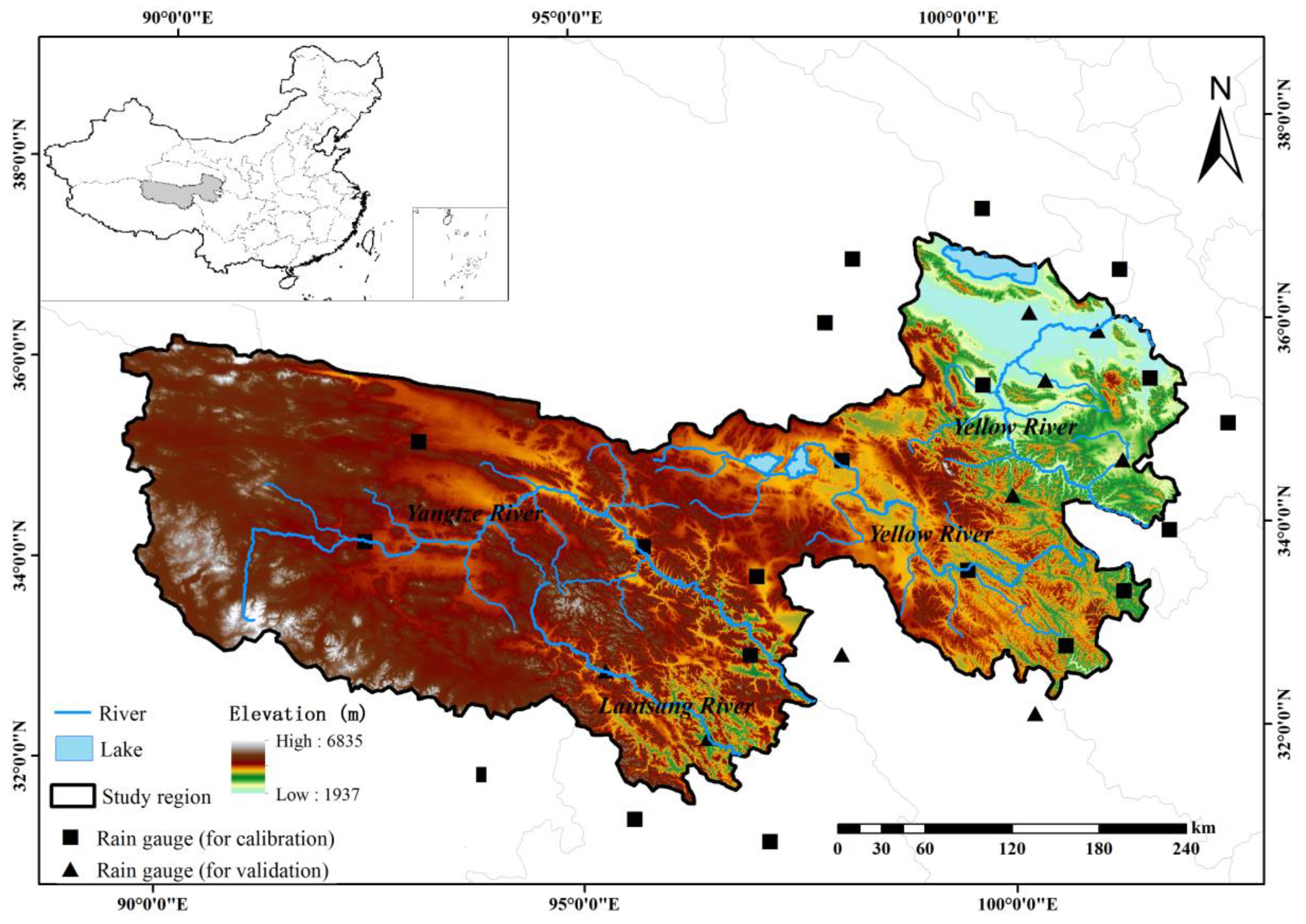
2.1. Study Area

The Three-River Headwaters region is located in the southern part of Qinghai Province in western China (31°39′–36°16′ N, 89°24′–102°23′ E), and is the source of the Yangtze River, Yellow River and Lantsang River, with a total area of approximately 360,000 km2 and an average altitude of more than 4000 m (Figure 1). The regional climate corresponds to the plateau continental climate; the elevation increases from southeast to northwest; the annual average temperature is between −5.6 and 7.8 °C [85]; and the annual average precipitation ranges from 262.2 to 772.8 mm [86]. The complex river systems in the region supply 25%, 49%, and 15% of the runoff the Yangtze River, Yellow River, and Lantsang River, respectively [87]. There are different soil types at low and high altitudes, including primarily alpine cold desert soil and alpine meadow soil [88], and the land cover is mainly meadow, steppe and alpine vegetation [11].

2.2. Data

2.2.1. Satellite Precipitation Dataset

The GPM Mission uses an international satellite network that provides a new generation of global rainfall and snowfall observations based on the TRMM. The core observation satellite, launched by the National Aeronautics and Space Administration (NASA) and the Japan Aerospace Exploration Agency (JAXA) in February 2014, carried the GPM Microwave Imager (GMI) and the Dual Frequency Precipitation Radar (DPR) [89]. Compared to TRMM data, it combined GPM, multiple satellite precipitation datasets, and microwave-calibrated infrared (IR) satellite estimates, and improved the ability to measure light rain and solid precipitation, resulting in higher-quality precipitation data. This study adopted the final half-hourly scale of GPM-3IMERGM precipitation data from 2010–2014 [90], covering a global scale with a spatial resolution of 0.1° × 0.1°. The dataset can be obtained from https://pmm.nasa.gov/data-access/downloads/gpm (accessed on 26 August 2022).
CMORPH is a global satellite precipitation data product developed by the CPC as part of the National Oceanic and Atmospheric Administration (NOAA) that estimates precipitation using microwave data from the U.S. Defense Weather Satellite, the U.S. Marine Weather Service, and the TRMM Microwave Radiometer. The coverage ranged from 60° S to 60° N, 180° E–180° W [13]. Currently, CMORPH offers two precipitation data products—one with 30 min and 8 km × 8 km resolutions, and the other with 3 h and 0.25° × 0.25° resolutions. In this paper, the 3 h scale, 0.25° CMORPH dataset in 2010–2014 was employed and data were accumulated as part of a daily scale. The information has been made publicly available at https://www.cpc.ncep.noaa.gov (accessed on 26 August 2022).
ERA5 is the latest fifth-generation global atmospheric reanalysis dataset of the ECMWF. It provided dozens of commonly used land-surface and atmospheric variables. It adopts data assimilation technology and integrates a large number of ground observations, atmospheric sounding data and remote sensing data [14]. In this paper, the hourly ERA5-land precipitation data in 2010 were selected with a spatial resolution of 0.1° × 0.1° and accumulated as daily scale data. The dataset is publicly available at https://cds.climate.copernicus.eu (accessed on 26 August 2022).
The cloud attribute data were obtained from the Moderate Resolution Image Spectrometer (MODIS) cloud product, MOD06/MYD06, developed by NASA, with a spatial resolution of 1 to 5 km, and can provide 1–4 images per day. The products (MOD06 and MYD06 for Terra and Aqua MODIS, respectively) combine infrared and visible light technologies to enable the pixel-level retrieval of cloud optical and physical properties based on unique spectral and spatial capabilities [72]. In this study, daily cloud product data with a spatial resolution of 1 km from the period of 2010–2014 were selected and accumulated on a daily scale. CER, COT, and CWP are auxiliary variables in the cloud product. The dataset is publicly accessible at https://ladsweb.modaps.eosdis.nasa.gov (accessed on 26 August 2022).

2.2.2. Rain Gauge Data
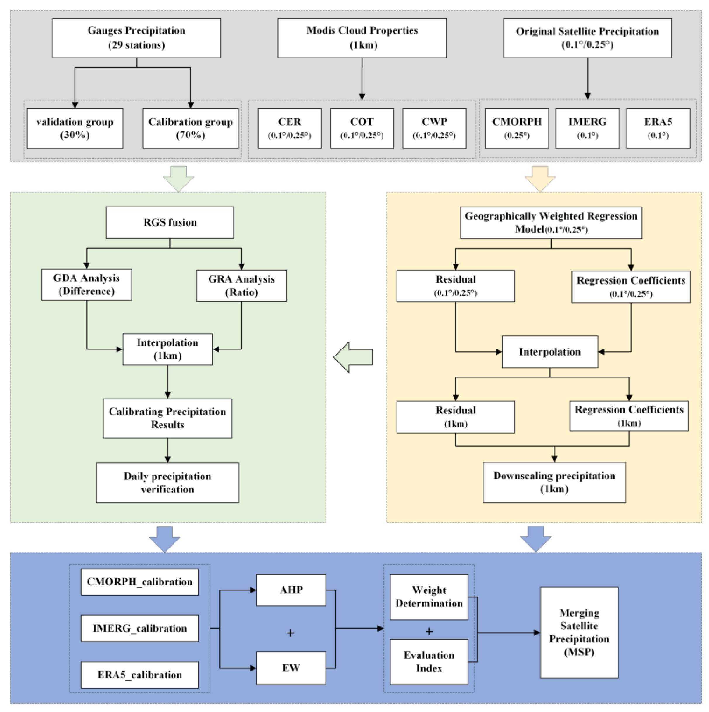
The daily scale rain gauge data from the China Meteorological Administration (CMA) were collected from the National Meteorological Science Data Center of China (http://data.cma.cn/ (accessed on 26 August 2022) to calibrate and validate the downscaled precipitation in this paper. The Chinese standard precipitation gauge (CSPG) was used to observe precipitation at 08:00 and 20:00 Beijing time every day. The precipitation data observed by meteorological stations will be released regularly with a lag of approximately three months for data compilation and quality control [91]. Due to the high altitude, complex terrain and inconvenient transportation in the Three-River Headwaters region, the available weather stations are sparse in and around the area. Although observed precipitation data at CMA weather stations are reliable, there are only 29 rain gauges in the area of 360,000 km2. Therefore, creating a gridded precipitation dataset for this region by simply interpolating the station observations to the grid points is not accurate [91]. As a result, it is necessary to combine station data with remote sensing datasets to obtain higher-quality precipitation data. In this study, the precipitation data collected at 20 stations and 9 stations were utilized to calibrate and validate the performance of downscaled precipitation, correspondingly. The spatial distribution of stations used in this study area is shown in Figure 1, and the basic information of selected stations is shown in Table 1.

2.3. Methodology

This section introduces the specific steps of the research method in this paper. The flow chart of the research scheme is shown in Figure 2, which mainly consists of the following two parts: downscaling and calibration. In the first step, based on the cloud optical attributes and the physical properties, namely CER, COT, and CWP, three satellite precipitation datasets, namely IMERG, CMORPH, and ERA5, were used to construct GWR models and were downscaled to a 1 km resolution, respectively. In the second step, based on the GDA and GRA methods, the downscaled satellite precipitation data were calibrated using the calibration group rain gauge data, and the inverse distance weight (IDW), ordinary kriging interpolation (OK) and radial basis function (RBF) were employed to interpolate the calibration residual results to a 1 km resolution and fused with the downscaled results to obtain three final satellite precipitation downscaling results. Finally, the validation group rain gauge data were used to evaluate the final precipitation downscaling result, and combined with the verification data. The AHP and EW method were employed to determine the weights to obtain the merged satellite precipitation (MSP) data.

2.3.1. Geographically Weighted Regression Models

Traditional regression models, such as the ordinary least square method, assume that the target variable and auxiliary variables are stationary over the entire region. Precipitation is the result of the interaction of various factors, and there exists typical spatial non-stationarity. The traditional global regression model could not reflect the spatial characteristics of precipitation. The GWR model is a regional regression method that can be used to construct non-stationary correlations between target and auxiliary variables [56]. The GWR model assumes that the regression coefficient varies with geographic location, and estimates the regression coefficient for each location and establishes a regression equation to explore spatial heterogeneity [59,92,93]. Its mathematical expression is as follows:
y i   = β 0 ( u i , v i ) + p = 1 j β p ( u i , v i )   x ip   + ε ( u i , v i ) i = 1 , 2 n
where yi is the precipitation at position i as a dependent variable; x ip is the observed value at position i of the p th auxiliary variable; ( u i , v i ) is the geographic coordinate at position I; β 0 ( u i , v i ) is the intercept at position I; β p ( u i , v i ) is the regression coefficient at position i, which is a function of geographic location; p is the number of auxiliary variables; and ε ( u i , v i ) is the independent normal distribution with zero mean errors.
The regression coefficient at position i can be estimated by solving the following matrix equation:
β ( u i , v i ) = ( X T ( W ( u i , v i ) ) X ) 1 X T W ( u i , v i ) y
where β ( u i , v i ) denotes the estimated local coefficient at position I; X and y are the auxiliary variables (cloud optical and physical properties) and dependent variable (precipitation); superscript T represents matrix transpose; and W ( u i , v i ) is the weight coefficient matrix, which mainly depends on the selection of the spatial kernel function [94]. It is vital to note in the GWR model that there is a linear dependence of the column vectors in X, i.e., a collinearity problem in terms of regression, which can cause errors in the solution of Equation (2) [1]. There are two main types of spatial kernel functions, namely the Gaussian function and Bi-square function.
(1)
Gaussian function
The Gaussian function uses a continuous monotonically decreasing function to describe the relationship between W ij and d ij . The mathematical relationship is expressed as follows:
W ij = exp ( ( d ij / b ) 2 )
where W ij is the observation weight at position j used to estimate the coefficient at position i; d ij is the distance between position i and position j; and b is the bandwidth, i.e., a non-negative attenuation parameter describing the relationship between the weight and the distance function [95], which could be confirmed by the Corrected Akaike Information Criterion (AICc) or cross-validation (CV) method.
(2)
Bi-square function
The Bi-square function may help to reduce the computational cost compared with the Gaussian function [86,90], and its expression is as follows:
W ij = { ( 1     ( d ij / b ) 2 ) 2   d ij     b 0   d ij   >   b  
The validation methods of adaptive bandwidth b mainly include AICc and CV methods. The AICc method is widely employed in the GWR model, which could be expressed as follows:
AICc = 2 Nlog e ( SSE N tr ( S ) ) + Nlog e ( 2 π ) + N ( N + tr ( S ) N 2 tr ( S ) )
where SSE represents the residual sum of squares, and tr(S) represents the trace of the hat matrix. The CV method expression is as follows:
CV = 1 n i = 1 n ( y i y ^ ( i ) ( b ) ) 2
where CV is the result of cross-validation, y i represents the observed value of the dependent variable at spatial position i; y ^ ( i ) ( b ) represents that in the case of bandwidth b, when estimating regression parameters, the regression calculation is performed only based on the observation points around position i. The Gaussian function and the AICc method were selected in this paper.
The GWR model downscaling algorithm assumes that the GWR relationship between precipitation and explanatory variables (CER, COT, and CWP) constructed at the original coarse resolution can be used to predict precipitation using the explanatory variables at higher resolutions. At the same time, due to the weak correlation between daily scale precipitation and environmental variables, we constructed a GWR model of cloud attributes and precipitation on the daily scale. Therefore, the specific steps of the downscaling algorithm in this study are as follows:
According to the resolutions of the three kinds of satellite precipitation data (IMERG: 0.1°, ERA5: 0.1°, and CMORPH: 0.25°), the three cloud attributes (CER, COT, CWP: 1 km) are resampled to the corresponding resolutions ( CER 0 . 25 ° , COT 0 . 25 ° , CWP 0 . 25 ° and CER 0 . 1 ° , COT 0 . 1 ° , CWP 0 . 1 ° ) by performing bilinear interpolation. Taking the resampled cloud attributes as auxiliary variables, a daily scale GWR model is constructed at the original resolution scale, and its expression is as follows:
P i , d original , SAT = β i , d SAT , 0 + β i , d SAT , 1 CER i , d SAT + β i , d SAT , 2 COT i , d SAT + β i , d SAT , 3 CWP i , d SAT + ε i , d original , SAT
where β i , d SAT , 0 , β i , d SAT , 1 , β i , d SAT , 2 and β i , d SAT , 3 are the regression coefficients of day d at position i (d = 1,2,3... 365 in 2010–2014), and ε i , d original , SAT represents the residual of day d at position i, respectively.   CER i , d SAT , COT i , d SAT , and CWP i , d SAT represent the corresponding resolution (0.1° and 0.25°) cloud attribute observations at position i, respectively, and P i , d original , SAT represents the observations of satellite precipitation data at the original resolution (0.1° and 0.25°).
By resampling the regression coefficients to a 1 km resolution, respectively, and establishing a GWR model on the 1 km scale to estimate the precipitation from satellite data with a 1 km resolution, the following expression is obtained:
P i , d 1   km , SAT = β i , d 1   km , SAT , 0   + β i , d 1   km , SAT , 1 CER i , d 1   km + β i , d 1   km , SAT , 2 COT i , d 1   km + β i , d 1   km , SAT , 3 CWP i , d 1   km
For the residual error generated in Equation (7) of the coarse-resolution GWR model, the IDW method is applied to interpolate it to a 1 km resolution ( ε i , d 1   km , SAT ) and fuse it with the 1 km resolution precipitation data estimated by Equation (8) to obtain the modified satellite precipitation data ( P ^ i , d 1   km , SAT ).
P ^ i , d 1   km , SAT = P i , d 1   km , SAT   + ε i , d 1   km , SAT  
It is worth noting that other researchers believe that the residuals generated by the GWR correlation model are spatially correlated and can be interpolated to help explain the spatial variation of the target variable [96,97]. In our fusion scheme, the residuals produced by the GWR model were interpolated to the downscaled precipitation resolution by employing an inverse distance weighted method and incorporated into the model estimate (residual correction) to improve prediction accuracy. In this study, after verifying the residual correction results of satellite downscaling, the data quality of IMERG and CMORPH improved to a certain extent, and ERA5 was negatively optimized. It is speculated that residual correction after precipitation downscaling is not applicable to ERA5 in this research scheme [33,53]. Therefore, in the follow-up research, in order to ensure the downscaling accuracy, ERA5, IMERG, and CMORPH are used to employ the downscaled precipitation data before and after residual correction, respectively, as the final precipitation downscaling result.

2.3.2. Geographic Difference Analysis and Geographic Ratio Analysis

Both GDA and GRA can be used to reduce the difference between satellite precipitation data and rain gauge measurement data [31,98]. In this study, we selected the validation group rain gauges (RGS) data to compare the calibration effect of GDA and GRA on downscaled data. The principle and expression are as follows:
(1)
Calculate the difference/ratio between downscaled precipitation and RGS measurements:
P ratio point = RGS / P i , d 1   km , SAT
P sub point = RGS P i , d 1   km , SAT
(2)
Interpolate the difference/ratio to 1 km resolution using interpolation techniques (GDA: IDW, Kriging, RBF; GRA: IDW).
(3)
Calibrate downscaled precipitation to obtain the final downscaled results:
P GRA 1   km , SAT = P i , d 1   km , SAT P ratio 1   km
P GDA 1   km , SAT   = P i , d 1   km , SAT + P sub 1   km
where P i , d 1   km , SAT represents the downscaled satellite precipitation data (CMORPH, ERA5, and IMERG), P sub 1   km is the difference interpolated to a 1 km resolution, P ratio 1   km is the difference ratio interpolated to a 1 km resolution, and P GRA 1   km , SAT and P GDA 1   km , SAT are the final downscale precipitation results.

2.3.3. Satellite Precipitation Data Fusion

The AHP method is a powerful and flexible decision theory, and it is the most commonly used subjective method to determine the weights of criteria/structures; it can also help researchers find the most suitable solution among numerous combination options [80,99,100]. Its main steps are as follows:
(1)
Construct a hierarchical structure, determine the judgment matrix according to the quality evaluation indicators and prior knowledge, and assign different values to represent the difference in the importance of the indicators.
(2)
Calculate the eigenvalues and eigenvectors of the judgment matrix:
λ max = 1 n i = 1 n ( X ω ) i ω i  
where λ max indicates the largest eigen value of the matrix,   ω indicates the weight vector, ω i indicates the weight of the i-th evaluation index, and n indicates the number of rating indicators.
(3)
Consistency verification:
CR = CI RI
where CR is the Consistency Ratio, and RI represents the average stochastic consistency index for the judgment matrix. The CI is the consistency index of the judgment matrix, which can be calculated using Equation (16):
CI = λ max     n n     1
where λ max is the largest eigen value of the matrix, and n is the number of indicators. If CR < 0.1, it means that the result has passed verification; otherwise, the judgment is inconsistent and the weight needs to be re-estimated.
AHP is widely employed in multidisciplinary fields, but its subjectivity is a disadvantage that cannot be ignored, which brings uncertainty to the results [101]. The EW method is currently used as the most common objective method for determining standard/structural weights [102]. EW does not consider information other than the data, and the determination of the weight of each indicator is based on the information of the data itself and the relationship between the indicators [103]. It reflects the amount of information provided by the indicator by calculating the information entropy of an indicator, so as to determine the role of the indicator in the comprehensive evaluation [104]. It can be implemented according to the following steps:
(1)
Standardize evaluation indicators.
Positive impact indicators:
Y ij   = X ij     min ( X ij ) max ( X ij )   min ( X ij )
Negative impact indicators:
Y ij = max ( X ij )   X ij max ( X ij )   min ( X ij )
where X ij is the value of the j-th evaluation indicator of the i-th evaluation object; and Y ij is the standardization of the standardization. max ( X ij ) and min ( X ij ) represent the maximum and minimum values of X ij , respectively.
(2)
Calculate indicator proportion:
P ij   = Y ij i = 1 n Y ij   i = 1 , 2 n ; j = 1 , 2 m
where P ij is the proportion of the indicator value of the j-th indicator of the first i-th evaluation object.
(3)
Calculate the entropy value and information entropy redundancy corresponding to each index as follows:
E j = 1 ln ( n ) i = 1 n P ij ln ( P ij )
D j   = 1   E j
where Ej is the entropy value of the j-th indicator, n is the value of the evaluation index number, and D j is the information entropy redundancy of the j-th indicator.
(4)
Calculate the weight of the indicator as follows:
ω j = D j j = 1 m D j
where ω j is the weight of index j, and m is the number of evaluation objects.
The weight obtained by a single evaluation method is not comprehensive. Combining subjective and objective methods does not only reflect the judgment of experts on the importance of indicators, but also objectively reflects the differences in actual data changes, making the evaluation results more appropriate to the real situation.
W j = ω j ω j j = 1 m ω j ω j
where W j denotes the comprehensive weight, ω j is the objective weight, and ω j is the subjective weight.

2.3.4. Validation

The effectiveness of the downscaling method is measured by using the following metrics: root mean square error (RMSE), BIAS (Bias) and Correlation Coefficient (CC). CC ranges from 0 to 1, with an optimal value of 1, which indicates the strength of the correlation between station observations and downscaled precipitation values. Bias describes the degree to which downscale precipitation estimates are over or underestimated, with an optimal value of 0. RMSE represents the size of the error estimate, and the smaller the RMSE, the more reliable the downscaled precipitation. Its mathematical expression is as follows:
CC = i = 1 N ( O i O _ i ) ( P i P _ i ) i = 1 N ( O i O _ i ) ( P i P _ i )
BIAS = i N P i i N O i     1
RMSE = i = 1 N ( P i     M i ) 2 N
where O i (mm) and P i (mm) are the observed precipitation and reduced precipitation at the location of the i-th weather station, respectively; O _ (mm) and P _ (mm) represent the mean values of O i and P i , respectively; N is the total number of values in the corresponding dataset.

3. Results

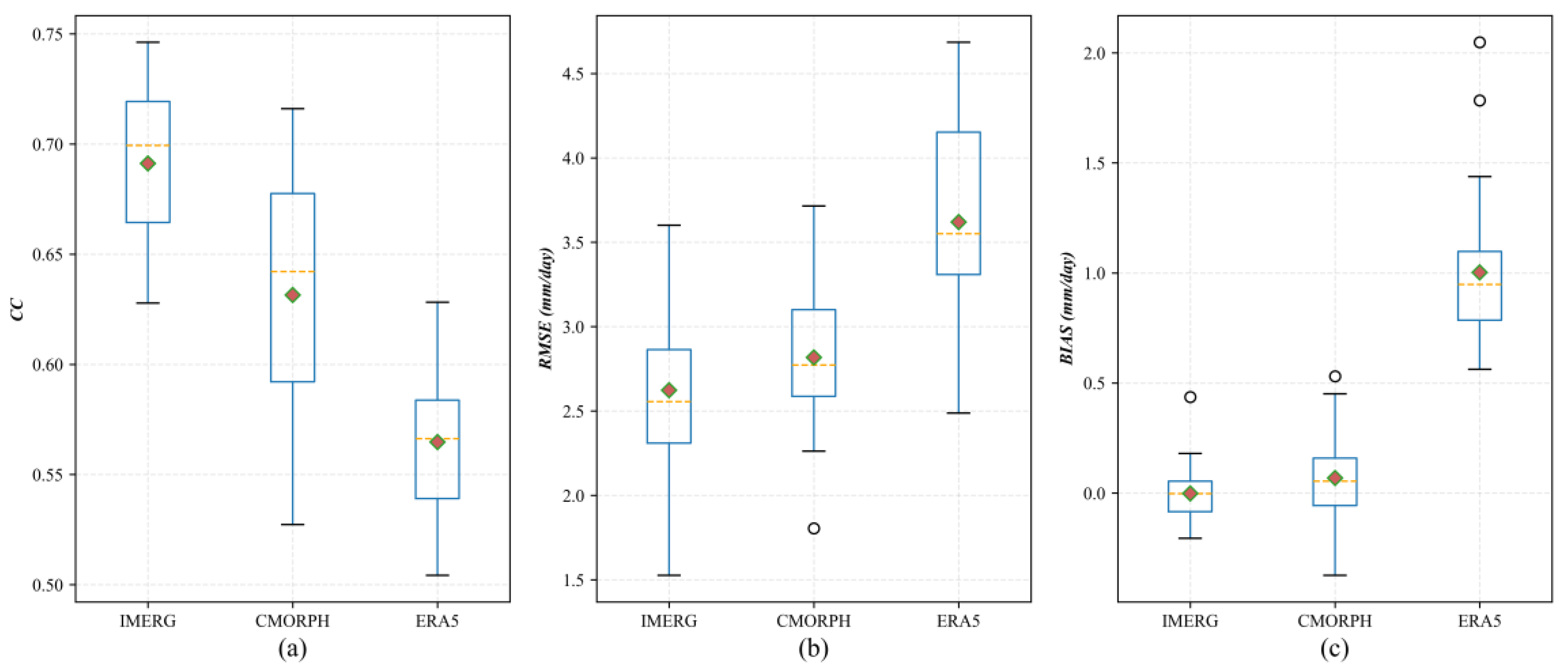
3.1. Accuracy of the Original Satellite Precipitation Dataset

The reliability of the raw satellite precipitation dataset is verified with observations from 29 rain gauges. According to the time when the daily precipitation data are obtained from the rain gauge results (8:00 p.m. the previous day to 8:00 p.m. on the current day), the obtained satellite precipitation data with original time resolution (30 min and 1 h) are converted according to Coordinated Universal Time (UTC) and Beijing time, and accumulated to the corresponding time period to obtain daily satellite precipitation data.
Figure 3 describes the relationship between original satellite precipitation and the rain gauge measurement value according to the daily time scale at one selected station location in the period of 2010–2014. The CC, BIAS and RMSE of these three satellite precipitation data and rain gauge data in the period of 2010–2014 are shown in Table 2. The CCs are as follows: 0.542 (ERA5), 0.615 (CMORPH), and 0.644 (IMERG), all of which pass the significance test at the 0.01 level, indicating that there is an obvious linear correlation and consistency between the three initial satellite rainfall data and rain gauge data. The BIAS results for CMORPH, IMERG, and ERA5 are 0.050, −0.013, and 0.885, respectively, implying that all three datasets overestimate or underestimate the precipitation to some extent compared with the RGS observations. Among them, the IMERG data are of the best quality. The lowest-scoring data quality was found for ERA5, which considerably overestimates precipitation.

3.2. The Relationship between Cloud Physical and Optical Properties and Precipitation

Before downscaling precipitation through the correlation between cloud attributes and satellite precipitation data, the correlations between selected auxiliary variables and three types of satellite data were analyzed, as shown in Table 3. The results shows that the CWP has the best correlation with the satellite precipitation data, and the lowest correlation was found for the CER. Among the satellite precipitation data, ERA5 and IMERG show a fine correlation with cloud attributes, and the CMORPH shows the weakest. It can be inferred that the GWR downscaling model constructed based on cloud attributes and satellite precipitation data should be better applied to ERA5 and IMERG. The validation of the precipitation downscaling results of the GWR model below also proves this.

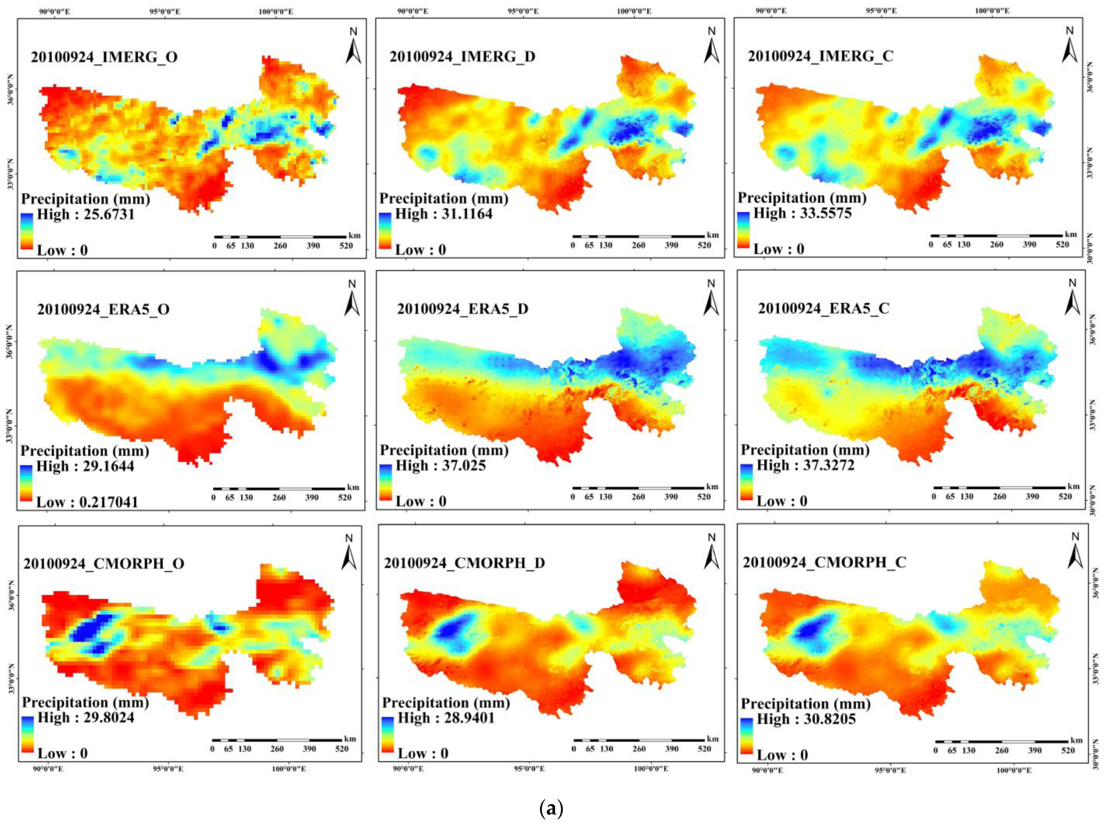
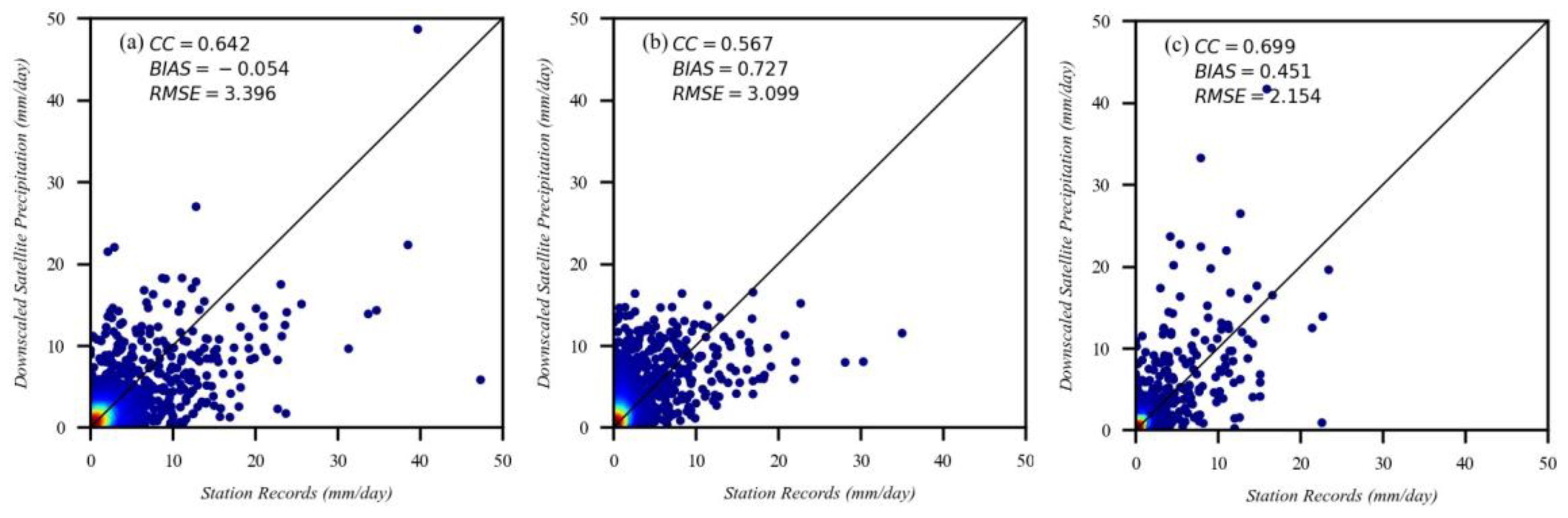
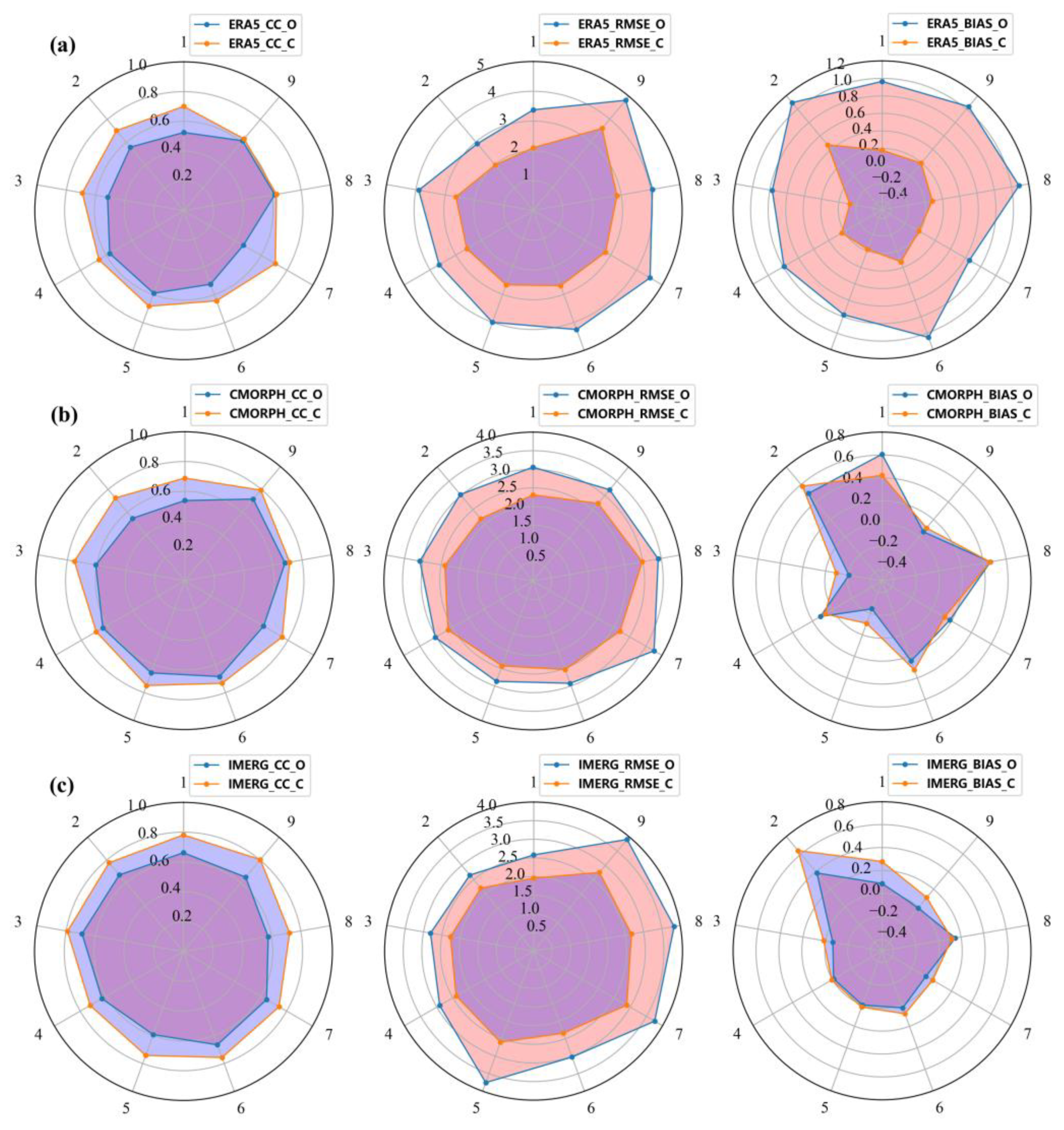
3.3. Evaluation of Downscaling Accuracy of Daily Scale Satellite Precipitation Datasets Based on GWR Model

The downscaled results of daily precipitation for three different satellites are shown in Figure 4, and the accuracy validation results with 29 rain gauge observations are shown in Table 4. Compared with original satellite data, the GWR model combines satellite-based precipitation observations with corresponding cloud properties, and the downscaled results improve the accuracy of precipitation data while reducing RMSE and BIAS (Table 4). Downscaled satellite precipitation based on cloud attributes describes spatial precipitation distribution in more detail at a 1 km resolution (Figure 5). After downscaling, the best correlation coefficients for CC are IMERG (CC: 0.691), the ones with the lowest RMSE and BIAS are also obtained for IMERG (IMERG_RMSE: 2.623 mm/day, IMERG_BIAS: 0.002 mm/day, respectively). The improvement of the three satellite precipitation data after downscaling are as follows: IMERG—CC from 0.644 to 0.691; CMORPH—CC from 0.615 to 0.631; and ERA5—CC from 0.542 to 0.565 (Table 4). These results also prove that our previous point of inferring the effect of downscaling based on the correlation between cloud attributes and different satellite precipitation data is correct. By analyzing the precision of the downscaled precipitation, it was found that the downscaled precipitation data obtained better data quality and smaller errors compared with the original satellite precipitation data (Figure 6). The quality of daily precipitation data after downscaling through the GWR model has improved; however, there is still an overestimation of the actual precipitation levels. Since the quality of downscaled predictions is restricted by the inherent precision of the original satellite precipitation product, it is vital to combine the downscaled precipitation data with the RGS data to improve the quality of the precipitation data.

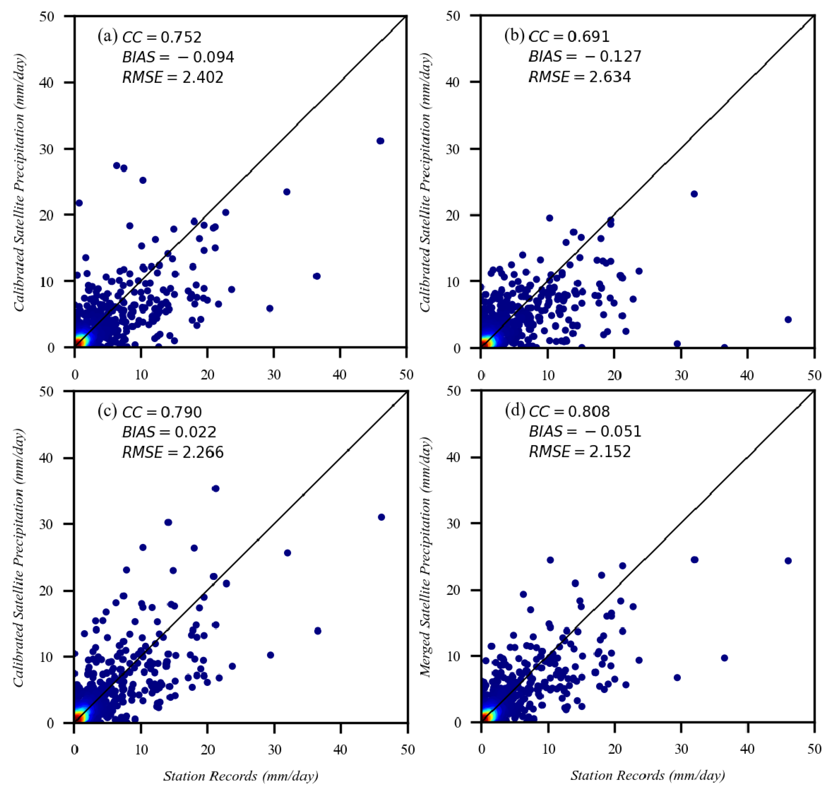
3.4. Data Fusion of Downscaled Precipitation with Rain Gauge Observations

Due to the difference between satellite precipitation data and RGS during downscaling, there may be a deviation between the downscaled data based on GWR and the actual precipitation. At the same time, owing to the difficulty of accessibility and the influence of other limiting factors, the observation of the data of rain gauges in high-altitude areas usually suffers from insufficient data acquisition. Therefore, the precipitation inferred from the observation data of rain gauges also has great uncertainty [105]. Therefore, the RGS data should be fused with the downscaled satellite precipitation data to obtain more accurate precipitation data. In this study, we employed two calibration methods based on RGS data, namely GDA and GRA. RGS data are divided into the following two groups: the calibration group (twenty stations) and validation group (nine stations).
Table 5 describes the validation statistics for three different satellite precipitation data calibrated with RGS over the entire time period and the original downscaled results before calibration. As shown in the analysis of the above results, both the GDA and GRA calibration methods could further improve the accuracy by increasing the CC and decreasing the RMSE and BIAS. There are differences in the calibration effects of GRA and GDA between various data sources. For the three kinds of satellite precipitation data, the calibration result of GDA is obviously better than that of GRA in the process of fusion RGS calibration. Figure 7 shows the comparison between the accuracy of the three satellite precipitation data after downscaling and the calibration of rain gauges and the accuracy of the original data. It can be concluded that the data quality after downscaling and rain gauge calibration has been significantly improved.
Similarly, the results of different interpolation methods (i.e., IDW, RBF, and OK) for GDA calibration are also quite different. Table 6 reveals the statistical results obtained by different interpolation methods when GDA calibrates the three satellite downscaled precipitation data. It can be found that among the three interpolation methods, GDA_RBF achieves better results in the calibration of CMORPH, IMERG and ERA5 downscaled data, and GDA_IDW performs well in the calibration of CMORPH downscaled data. The calibration result of GDA_OK is more common. In general, the ERA5 data have the lowest original accuracy, but the data quality improvement after downscaling and rain gauge calibration is the highest. While maintaining the highest raw accuracy, the IMERG data displays a good response to GWR downscaling and rain gauge calibration operations and achieves optimal data results. CMORPH data have high raw data precision and fine downscaling and calibration results, but they are not sensitive to the GWR downscaling method based on cloud attributes. GDA_RBF performs best in the calibration verification process of downscaled satellite data based on RGS.

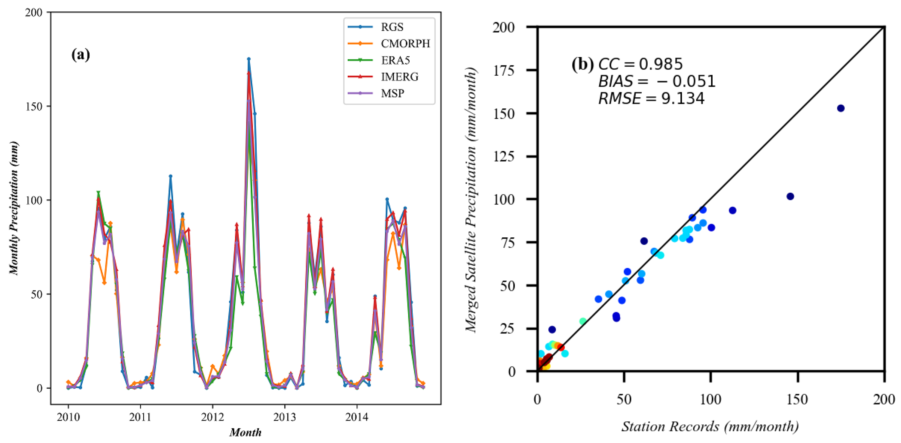
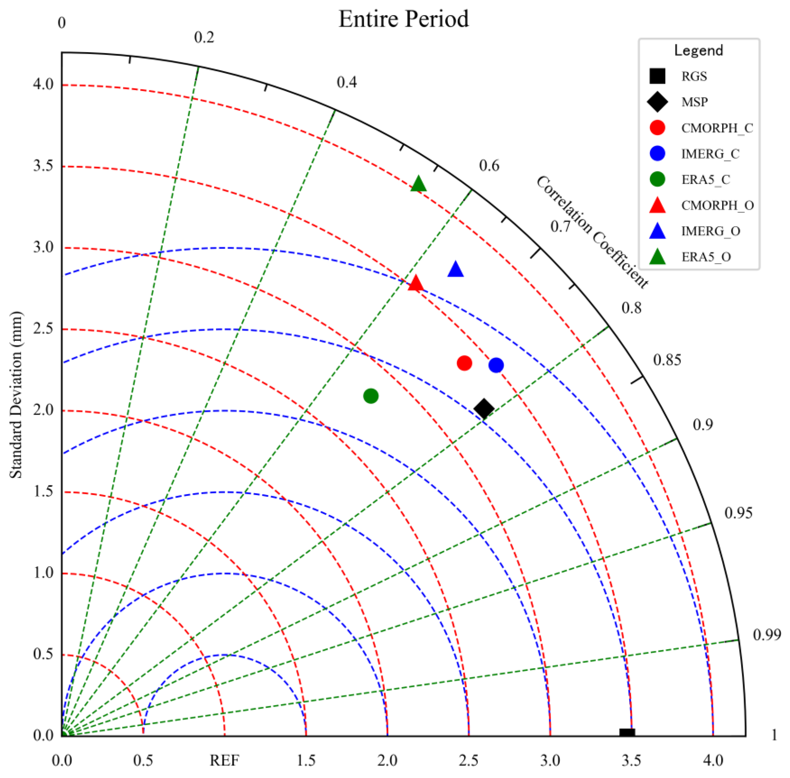
3.5. Performance of the Merged Satellite Precipitation

In this paper, based on three kinds of calibration data and quality evaluation indicators, different methods, including the principal component analysis (PCA), EW, AHP, and fusion of AHP and EW, were used to determine the weight of the target point and promote the whole region to merge multi-source satellite calibration data. Figure 8 and Figure 9 and Table 7 show the accuracy changes in different calibration data and multiple fusion data from 2010 to 2014. As one of the most widely used weight determination method, the EW method results are better than those of AHP and PCA; however, the performance of the EW method is worse than the subjective and objective weighting method that combines AHP and EW, which is consistent with the results in the literature [106,107]. It can be concluded that the merged satellite precipitation data, obtained when fusing AHP with EW, provide the most accurate estimation on a diurnal scale compared to calibration data and other fused data due to their lower RMSE and BIAS values (RMSE = 2.189 mm, BIAS = 0.142 mm); furthermore, the CC value (CC = 0.790) is higher than in the calibration data and any other fused precipitation product. The results show that the data fusion technique can significantly reduce the systematic error [108]. They also prove the applicability of the subjective and objective weighting method combined with the AHP and EW method, as introduced in this study in the fusion of multi-source satellite calibration data.
PCA, EW, and AHP, as the most widely used methods for determining the weighting of data structures, have shown superior performance in different scientific fields [100,109]; however, in this research, their performances seem to be weaker than that of the subjective and objective weighting method combining AHP and EW, which may be because individually they only consider the amount of data information or the prior knowledge of experts [110]. Although the subjective and objective weighting method has achieved the best fusion results, it needs to combine the AHP and EW methods to determine the weight. The associated time cost and calculation cost are also higher than for other weighting methods [106,111].

3.6. Temporal and Spatial Characteristics of Precipitation Data

Figure 10 indicates the calibrated annual precipitation of the three satellite precipitation data and the merged annual precipitation. Figure 10 shows the calibrated and merged monthly cumulative precipitation changes in different satellite precipitation data during the study period, and the correlation analysis between MSP monthly precipitation and rain gauge data, respectively. From the above image analysis, the calibrated and merged satellite precipitation based on the three satellite data show similar spatial trends to the original satellite precipitation estimates. There is greater precipitation in the southeast and less in the northwest. Precipitation decreases from southeast to northwest, consistent with the influence of the southeast monsoon. Compared with the coarse resolution of the original satellite data, both the calibrated and merged satellite precipitation results show a greater amount of spatial detail and more obvious local spatial variation; furthermore, the merged satellite precipitation data provide more complete precipitation spatial information than single satellite precipitation data, and the precipitation distribution is more accurate (Figure 10) [27]. It is worth noting that, according to the previous article and the interannual precipitation cumulative distribution map, it can be concluded that the spatial variation of the downscaled and the merged satellite precipitation is more in line with the real precipitation distribution.
From the monthly cumulative precipitation results, it could be concluded that the downscaled and calibrated precipitation has a consistent correlation with the rain gauge observations (Figure 11). The quality of the calibrated monthly cumulative satellite precipitation data has also been improved (ERA5: CC from 0.925 to 0.945, CMORPH: CC from 0.895 to 0.951, IMERG: CC from 0.967 to 0.971, MSP: CC = 0.969). Areas with a higher level of precipitation after downscaling and calibration also have greater levels of actual precipitation. Rainfall overestimation mainly occurs in periods of sufficient precipitation (summer). The merged satellite precipitation corrects the original satellite data to a certain extent, thereby reducing the difference between it and the rain gauge observation data, meaning the merged precipitation data are more accurate.
The result of the merged satellite precipitation data is influenced by elevation. As shown in Table 8, among the nine rain gauges in the validation group, the average CC of rain gauges above 3500 m is 0.783, and the average CC of rain gauges below 3500 m is 0.80. The results demonstrate that the downscaling, calibration and merging effect of precipitation data basically presents a trend of worsening quality with the increase in altitude. On the one hand, due to the sparse and uneven distribution of rain gauges in high-altitude areas, it is hard to satisfy the needs of rain gauge calibration. On the other hand, the estimation of precipitation data by satellites in high-altitude areas is influenced by the terrain and other complex environmental and climatic factors [112].

4. Discussion

4.1. Feasibility of a GWR Downscaling Model Based on the Correlation between Cloud Attributes and Daily Precipitation Data

The relationship between precipitation and the environment is spatially heterogeneous and scale dependent, especially in mountainous areas with a dramatic topography [33]. Therefore, considering the relationship between precipitation and the spatial variation of environmental variables, it may be more appropriate to establish a local regression downscaling model than a global regression downscaling model. The GWR model describes the relationship between precipitation and auxiliary environmental variables by means of local regression, and has been widely used in satellite precipitation data downscaling. Auxiliary environmental variables such as elevation, terrain, slope, latitude and longitude, and NDVI are adopted to construct the GWR precipitation downscaling model to downscale the annual and monthly satellite precipitation data [4,49,56,60,112].
However, few studies have directly constructed GWR models through daily scale environmental variables and precipitation to downscale daily scale precipitation data. Relevant studies have shown that the correlation between cloud attribute data and precipitation is useful in achieving precipitation downscaling [71,72]. Therefore, this study selects the daily cloud attributes, and realizes daily scale precipitation downscaling according to the local regression relationship between them and precipitation, which is of significant importance. The traditional method for obtaining daily and monthly precipitation is to employ the daily fraction and monthly fraction methods [30]. This method mainly relies on the accuracy of the original satellite precipitation data, and there are uncertainties. This paper introduces cloud attribute variables based on the accuracy of the original satellite data, which improves the reliability of daily scale precipitation downscaling to a certain extent. At the same time, after introducing cloud attributes as auxiliary environmental variables in the GWR model, the quality of the three satellite downscale precipitation data improved, which also proves the universality and feasibility of this research scheme.
By constructing the GWR model of cloud attributes and precipitation data, we obtain downscaled satellite precipitation data as the basic data, which also reduces the impact of the original satellite data errors in the GDA and GRA methods, as shown in Figure 11. Simultaneously, the GDA and GRA methods that integrate the rain gauge observation data further improve the quality of the downscaled precipitation data.

4.2. Evaluation of Merged Satellite Precipitation

Fusion methods based on different datasets or different members of the same model could be used to effectively reduce estimation uncertainty in meteorology and hydrology [113]. Typically, merged datasets contain information about multiple members and possess superior data quality than any single dataset [114,115]. The basic data commonly used for precipitation data fusion are mostly raw satellite data with low precision and rough resolution, which has a great impact on the quality and application of the final fusion data. In this paper, the precipitation data obtained after downscaling and calibration are selected, which is also an essential factor for obtaining the final high-quality precipitation data.
On this basis, the AHP and EW method are combined to merge different satellite precipitation data. This method not only incorporates experts’ experience and prior knowledge, but also includes the correlation between data information and evaluation indicators. The use of this method is critical to obtain more reasonable results (Figure 12).

4.3. Sources of Error and Uncertainty in GWR Downscaling Models

The GWR precipitation downscaling model calibrated with rain gauge data has achieved good results in the Three-River Headwaters region, but there are still some uncertainties and errors that limit the improvement of the quality of downscaled precipitation data. Spatial precipitation downscaling assumes that the regression relationship between precipitation and auxiliary variables constructed under coarse-scale conditions is still applicable at a fine scale. However, there are regional and seasonal deviations in the original satellite precipitation data [29,116], which may seriously interfere with the relationship between precipitation at coarse-resolution scales and auxiliary environmental variables, and further affect the precision of precipitation at the fine scale. For example, in the ERA5 data selected in this paper, there is a serious overestimation of the precipitation data, which limits its quality improvement in the downscaling process to a certain extent. At the same time, when performing residual correction on some downscaled precipitation data in this study, the results show that the correction effect has a negative optimization phenomenon [33], which indicates that the model residual correction after downscaling should be discussed. According to this paper, we speculate that it may be the influence of the spatial density and residual spatial structure of satellite precipitation data.
In the process of spatial precipitation downscaling, the calibration of rain gauge observations is essential. Studies have shown that the number of rain gauges plays a critical role in the calibration of precipitation downscaling models [31,117,118]. GDA and GRA have been widely used and proved to be of great significance in reducing precipitation downscaling errors. The sparse distribution of rain gauges and the high elevation of the region often influence the acquisition of precipitation data, meaning the calibration results of GDA and GRA are lower than expected. The Three-River Headwaters region covers an area of 360,000 square kilometers, with an average elevation of more than 4000 m. Only 29 rain gauge data are available, which greatly increases the difficulty of precipitation downscaling and calibration in this region. At the same time, some of the MODIS cloud attribution data were missing; therefore, the data does not completely cover the entire time period in the study area, which also has a certain impact on the results of the precipitation downscaling model.

4.4. Directions for Future Research Improvement

In the future, further improvement of the daily scale satellite precipitation downscaling model, incorporating the calibration of rain gauges, could be achieved by taking the following factors into consideration. First, the correlation between some other auxiliary environmental variables and precipitation should be considered as much as possible to construct a daily scale for the GWR model to achieve precipitation downscaling, such as soil moisture, evapotranspiration, temperature, humidity, and atmospheric circulation [4,119]. In addition, related studies have shown that, based on the linear relationship between cloud attributes and precipitation, hourly or sub-hourly precipitation downscaling could be achieved to satisfy the multi-scale application of precipitation data, which should be the focus of future research [73]. At the same time, the errors in the original satellite precipitation products should not be ignored; they can instead be discussed by combining the bias-corrected satellite estimates with rain gauge observations [64]. Secondly, according to the above research results, the GWR downscaling calibration model illustrates various downscaling accuracies at different geographical locations. For example, the altitude has a significant influence on the downscaling calibration results [112], and the GWR model should be further improved and developed to resolve related issues. Finally, the introduction of auxiliary variables and multi-source satellite data, coupled with numerical weather prediction (NWP) models, and the development of new data fusion algorithms and precipitation data fusion models referenced by auxiliary variables are conducive to improving the quality of precipitation products [1,74].

5. Conclusions

In this study, a daily scale GWR precipitation downscaling model based on the correlation between cloud optical, physical properties (CER, COT, and CWP) and precipitation is proposed. Three different types of satellite precipitation data (i.e., CMORPH, IMERG, and ERA5) were used for downscaling (from 0.25° and 0.1° to 1 km). Based on the downscaled results, the GDA and GRA methods were employed to integrate rainfall data for calibration and verification. Meanwhile, the subjective and objective weighting method combining AHP and EW was adopted to merge multi-source satellite calibration data to further improve the quality of the precipitation data products. The scheme was applied to the Three-River Headwaters region for the period of 2010–2014, and the research results are as follows.
The three kinds of original satellite precipitation data and rain gauge data have an obvious linear correlation and consistency (CC: 0.542, 0.615, and 0.644, respectively); however, there were various levels of underestimation or overestimation of the actual precipitation.
Among the original satellite data, ERA5 and IMERG had good correlation with cloud attributes, and the data quality was significantly improved after downscaling (IMERG: CC from 0.644 to 0.691, and ERA5: CC from 0.542 to 0.565). The remaining satellite data were also improved on the basis of the original data accuracy (CMORPH: CC from 0.615 to 0.631), which indicates that it is feasible to construct a GWR model of the correlation between cloud attributes and precipitation on a daily scale. This also demonstrates the applicability of this model to various satellite data.
The calibration and validation of downscaled precipitation with integrated rain gauge data are critical steps to help improve the quality of downscaled precipitation data. After the calibration and validation of the downscaling results of different satellite precipitation data using GDA and GRA methods, the accuracy of the downscaling results was significantly improved (IMERG: CC from 0.691 to 0.760, CMORPH: CC from 0.631 to 0.733, and ERA5: CC from 0.565 to 0.672). The IMERG data achieved the best downscaling and calibration results. For different satellite data, the GDA method obtained the optimal calibration results compared with the GRA method. In this study, the GDA_RBF method was better.
In the fusion step, considering the data quality evaluation index, the subjective and objective weighting method combining AHP and EW was adopted to merge the multi-source satellite-calibrated precipitation data. Compared with any single-satellite calibrated precipitation datum, the merged satellite precipitation had better performance (CC = 0.790, RMSE = 2.189 mm/day, and BIAS = 0.142 mm).
In summary, the solution proposed in this research based on the daily scale cloud attribute, precipitation GWR downscaling model and the fusion rain gauge calibration scheme is applicable in the Three-River Headwaters region, which has a complex terrain and harsh climatic conditions. At the same time, the combination of AHP and EW in the multi-source satellite data fusion technology method utilized in this paper further improved the quality of daily scale satellite precipitation data in the study area.

Author Contributions

Conceptualization, W.Z.; methodology, C.X. and C.L.; software, C.X. and C.L.; validation, C.X. and C.L.; data curation, Z.L. and B.A.; writing—original draft preparation, C.X. and C.L.; writing—review and editing, W.Z.; supervision, W.Z. All authors have read and agreed to the published version of the manuscript.

Funding

This research was jointly funded by the Innovative Research Program of the International Research Center of Big Data for Sustainable Development Goals [Grant No. CBAS2022IRP08] and the Key R&D and Transformation Program of Qinghai Province [Grant No. 2020-SF-C37].

Data Availability Statement

The data presented in this study are available on request from the corresponding author.

Conflicts of Interest

The authors declare no conflict of interest.

References

  1. Chen, S.; Xiong, L.; Ma, Q.; Kim, J.-S.; Chen, J.; Xu, C.-Y. Improving Daily Spatial Precipitation Estimates by Merging Gauge Observation with Multiple Satellite-Based Precipitation Products Based on the Geographically Weighted Ridge Regression Method. J. Hydrol. 2020, 589, 125156. [Google Scholar] [CrossRef]
  2. Hussain, Y.; Satgé, F.; Hussain, M.B.; Martinez-Carvajal, H.; Bonnet, M.-P.; Cárdenas-Soto, M.; Roig, H.L.; Akhter, G. Performance of CMORPH, TMPA, and PERSIANN Rainfall Datasets over Plain, Mountainous, and Glacial Regions of Pakistan. Theor. Appl. Climatol. 2018, 131, 1119–1132. [Google Scholar] [CrossRef]
  3. Bohnenstengel, S.I.; Schlünzen, K.H.; Beyrich, F. Representativity of in Situ Precipitation Measurements—A Case Study for the LITFASS Area in North-Eastern Germany. J. Hydrol. 2011, 400, 387–395. [Google Scholar] [CrossRef]
  4. Arshad, A.; Zhang, W.; Zhang, Z.; Wang, S.; Zhang, B.; Cheema, M.J.M.; Shalamzari, M.J. Reconstructing High-Resolution Gridded Precipitation Data Using an Improved Downscaling Approach over the High Altitude Mountain Regions of Upper Indus Basin (UIB). Sci. Total Environ. 2021, 784, 147140. [Google Scholar] [CrossRef]
  5. Wang, S.; Xu, C.; Zhang, W.; Chen, H.; Zhang, B. Human-Induced Water Loss from Closed Inland Lakes: Hydrological Simulations in China’s Daihai Lake. J. Hydrol. 2022, 607, 127552. [Google Scholar] [CrossRef]
  6. Gao, Z.; Long, D.; Tang, G.; Zeng, C.; Huang, J.; Hong, Y. Assessing the Potential of Satellite-Based Precipitation Estimates for Flood Frequency Analysis in Ungauged or Poorly Gauged Tributaries of China’s Yangtze River Basin. J. Hydrol. 2017, 550, 478–496. [Google Scholar] [CrossRef]
  7. Jiang, S.; Ren, L.; Hong, Y.; Yong, B.; Yang, X.; Yuan, F.; Ma, M. Comprehensive Evaluation of Multi-Satellite Precipitation Products with a Dense Rain Gauge Network and Optimally Merging Their Simulated Hydrological Flows Using the Bayesian Model Averaging Method. J. Hydrol. 2012, 452–453, 213–225. [Google Scholar] [CrossRef]
  8. Aslami, F.; Ghorbani, A.; Sobhani, B.; Esmali, A. Comprehensive Comparison of Daily IMERG and GSMaP Satellite Precipitation Products in Ardabil Province, Iran. Int. J. Remote Sens. 2019, 40, 3139–3153. [Google Scholar] [CrossRef]
  9. Skaugen, T.; Andersen, J. Simulated Precipitation Fields with Variance-Consistent Interpolation. Hydrol. Sci. J. 2010, 55, 676–686. [Google Scholar] [CrossRef] [Green Version]
  10. Darand, M.; Amanollahi, J.; Zandkarimi, S. Evaluation of the Performance of TRMM Multi-Satellite Precipitation Analysis (TMPA) Estimation over Iran. Atmospheric Res. 2017, 190, 121–127. [Google Scholar] [CrossRef]
  11. Zhang, T.; Li, B.; Yuan, Y.; Gao, X.; Sun, Q.; Xu, L.; Jiang, Y. Spatial Downscaling of TRMM Precipitation Data Considering the Impacts of Macro-Geographical Factors and Local Elevation in the Three-River Headwaters Region. Remote Sens. Environ. 2018, 215, 109–127. [Google Scholar] [CrossRef]
  12. Huffman, G.J.; Bolvin, D.T.; Nelkin, E.J.; Wolff, D.B.; Adler, R.F.; Gu, G.; Hong, Y.; Bowman, K.P.; Stocker, E.F. The TRMM Multisatellite Precipitation Analysis (TMPA): Quasi-Global, Multiyear, Combined-Sensor Precipitation Estimates at Fine Scales. J. Hydrometeorol. 2007, 8, 38–55. [Google Scholar] [CrossRef]
  13. Joyce, R.J.; Janowiak, J.E.; Arkin, P.A.; Xie, P. CMORPH: A Method That Produces Global Precipitation Estimates from Passive Microwave and Infrared Data at High Spatial and Temporal Resolution. J. Hydrometeorol. 2004, 5, 487–503. [Google Scholar] [CrossRef]
  14. Hersbach, H.; Bell, B.; Berrisford, P.; Hirahara, S.; Horányi, A.; Muñoz-Sabater, J.; Nicolas, J.; Peubey, C.; Radu, R.; Schepers, D.; et al. The ERA5 Global Reanalysis. Q. J. R. Meteorol. Soc. 2020, 146, 1999–2049. [Google Scholar] [CrossRef]
  15. Ushio, T.; Sasashige, K.; Kubota, T.; Shige, S.; Okamoto, K.; Aonashi, K.; Inoue, T.; Takahashi, N.; Iguchi, T.; Kachi, M.; et al. A Kalman Filter Approach to the Global Satellite Mapping of Precipitation (GSMaP) from Combined Passive Microwave and Infrared Radiometric Data. J. Meteorol. Soc. Jpn. Ser II 2009, 87A, 137–151. [Google Scholar] [CrossRef] [Green Version]
  16. Huffman, G.J.; Adler, R.F.; Bolvin, D.T.; Gu, G. Improving the Global Precipitation Record: GPCP Version 2.1. Geophys. Res. Lett. 2009, 36, L17808. [Google Scholar] [CrossRef] [Green Version]
  17. Huffman, G.J.; Adler, R.F.; Arkin, P.; Chang, A.; Ferraro, R.; Gruber, A.; Janowiak, J.; McNab, A.; Rudolf, B.; Schneider, U. The Global Precipitation Climatology Project (GPCP) Combined Precipitation Dataset. Bull. Am. Meteorol. Soc. 1997, 78, 5–20. [Google Scholar] [CrossRef]
  18. Ashouri, H.; Hsu, K.-L.; Sorooshian, S.; Braithwaite, D.K.; Knapp, K.R.; Cecil, L.D.; Nelson, B.R.; Prat, O.P. PERSIANN-CDR: Daily Precipitation Climate Data Record from Multisatellite Observations for Hydrological and Climate Studies. Bull. Am. Meteorol. Soc. 2015, 96, 69–83. [Google Scholar] [CrossRef] [Green Version]
  19. Liu, J.; Zhang, W.; Nie, N. Spatial Downscaling of TRMM Precipitation Data Using an Optimal Subset Regression Model with NDVI and Terrain Factors in the Yarlung Zangbo River Basin, China. Adv. Meteorol. 2018, 2018, 3491960. [Google Scholar] [CrossRef] [Green Version]
  20. Zhan, C.; Han, J.; Hu, S.; Liu, L.; Dong, Y. Spatial Downscaling of GPM Annual and Monthly Precipitation Using Regression-Based Algorithms in a Mountainous Area. Adv. Meteorol. 2018, 2018, 1506017. [Google Scholar] [CrossRef] [Green Version]
  21. Massari, C.; Crow, W.; Brocca, L. An Assessment of the Performance of Global Rainfall Estimates without Ground-Based Observations. Hydrol. Earth Syst. Sci. 2017, 21, 4347–4361. [Google Scholar] [CrossRef] [Green Version]
  22. Li, L.; Hong, Y.; Wang, J.; Adler, R.F.; Policelli, F.S.; Habib, S.; Irwn, D.; Korme, T.; Okello, L. Evaluation of the Real-Time TRMM-Based Multi-Satellite Precipitation Analysis for an Operational Flood Prediction System in Nzoia Basin, Lake Victoria, Africa. Nat. Hazards 2009, 50, 109–123. [Google Scholar] [CrossRef]
  23. Ringard, J.; Becker, M.; Seyler, F.; Linguet, L. Temporal and Spatial Assessment of Four Satellite Rainfall Estimates over French Guiana and North Brazil. Remote Sens. 2015, 7, 16441–16459. [Google Scholar] [CrossRef] [Green Version]
  24. Sohn, B.J.; Han, H.-J.; Seo, E.-K. Validation of Satellite-Based High-Resolution Rainfall Products over the Korean Peninsula Using Data from a Dense Rain Gauge Network. J. Appl. Meteorol. Climatol. 2010, 49, 701–714. [Google Scholar] [CrossRef]
  25. Tong, K.; Su, F.; Yang, D.; Hao, Z. Evaluation of Satellite Precipitation Retrievals and Their Potential Utilities in Hydrologic Modeling over the Tibetan Plateau. J. Hydrol. 2014, 519, 423–437. [Google Scholar] [CrossRef]
  26. Wang, W.; Lu, H.; Yang, D.; Sothea, K.; Jiao, Y.; Gao, B.; Peng, X.; Pang, Z. Modelling Hydrologic Processes in the Mekong River Basin Using a Distributed Model Driven by Satellite Precipitation and Rain Gauge Observations. PLoS ONE 2016, 11, e0152229. [Google Scholar] [CrossRef] [Green Version]
  27. Yaduvanshi, A.; Srivastava, P.K.; Pandey, A.C. Integrating TRMM and MODIS Satellite with Socio-Economic Vulnerability for Monitoring Drought Risk over a Tropical Region of India. Phys. Chem. Earth Parts ABC 2015, 83–84, 14–27. [Google Scholar] [CrossRef]
  28. Tang, G.; Clark, M.P.; Papalexiou, S.M.; Ma, Z.; Hong, Y. Have Satellite Precipitation Products Improved over Last Two Decades? A Comprehensive Comparison of GPM IMERG with Nine Satellite and Reanalysis Datasets. Remote Sens. Environ. 2020, 240, 111697. [Google Scholar] [CrossRef]
  29. Maggioni, V.; Meyers, P.C.; Robinson, M.D. A Review of Merged High-Resolution Satellite Precipitation Product Accuracy during the Tropical Rainfall Measuring Mission (TRMM) Era. J. Hydrometeorol. 2016, 17, 1101–1117. [Google Scholar] [CrossRef]
  30. Sun, Q.; Miao, C.; Duan, Q.; Ashouri, H.; Sorooshian, S.; Hsu, K. A Review of Global Precipitation Data Sets: Data Sources, Estimation, and Intercomparisons. Rev. Geophys. 2018, 56, 79–107. [Google Scholar] [CrossRef] [Green Version]
  31. Duan, Z.; Bastiaanssen, W.G.M. First Results from Version 7 TRMM 3B43 Precipitation Product in Combination with a New Downscaling–Calibration Procedure. Remote Sens. Environ. 2013, 131, 1–13. [Google Scholar] [CrossRef]
  32. Ma, Z.; Tan, X.; Yang, Y.; Chen, X.; Kan, G.; Ji, X.; Lu, H.; Long, J.; Cui, Y.; Hong, Y. The First Comparisons of IMERG and the Downscaled Results Based on IMERG in Hydrological Utility over the Ganjiang River Basin. Water 2018, 10, 1392. [Google Scholar] [CrossRef] [Green Version]
  33. Xu, S.; Wu, C.; Wang, L.; Gonsamo, A.; Shen, Y.; Niu, Z. A New Satellite-Based Monthly Precipitation Downscaling Algorithm with Non-Stationary Relationship between Precipitation and Land Surface Characteristics. Remote Sens. Environ. 2015, 162, 119–140. [Google Scholar] [CrossRef]
  34. Hong, Y.; Hsu, K.-L.; Sorooshian, S.; Gao, X. Precipitation Estimation from Remotely Sensed Imagery Using an Artificial Neural Network Cloud Classification System. J. Appl. Meteorol. 2004, 43, 1834–1853. [Google Scholar] [CrossRef] [Green Version]
  35. Tegos, A.; Ziogas, A.; Bellos, V.; Tzimas, A. Forensic Hydrology: A Complete Reconstruction of an Extreme Flood Event in Data-Scarce Area. Hydrology 2022, 9, 93. [Google Scholar] [CrossRef]
  36. Ma, Z.; Zhou, Y.; Hu, B.; Liang, Z.; Shi, Z. Downscaling Annual Precipitation with TMPA and Land Surface Characteristics in China. Int. J. Climatol. 2017, 37, 5107–5119. [Google Scholar] [CrossRef]
  37. Zhang, S.; Wang, D.; Qin, Z.; Zheng, Y.; Guo, J. Assessment of the GPM and TRMM Precipitation Products Using the Rain Gauge Network over the Tibetan Plateau. J. Meteorol. Res. 2018, 32, 324–336. [Google Scholar] [CrossRef]
  38. Zhang, T.; Yang, Y.; Dong, Z.; Gui, S. A Multiscale Assessment of Three Satellite Precipitation Products (TRMM, CMORPH, and PERSIANN) in the Three Gorges Reservoir Area in China. Adv. Meteorol. 2021, 2021, 9979216. [Google Scholar] [CrossRef]
  39. Tang, G.; Long, D.; Hong, Y. Systematic Anomalies Over Inland Water Bodies of High Mountain Asia in TRMM Precipitation Estimates: No Longer a Problem for the GPM Era? IEEE Geosci. Remote Sens. Lett. 2016, 13, 1762–1766. [Google Scholar] [CrossRef]
  40. Shen, Y.; Xiong, A.; Wang, Y.; Xie, P. Performance of High-Resolution Satellite Precipitation Products over China. J. Geophys. Res. 2010, 115, D02114. [Google Scholar] [CrossRef]
  41. Nashwan, M.S.; Shahid, S.; Dewan, A.; Ismail, T.; Alias, N. Performance of Five High Resolution Satellite-Based Precipitation Products in Arid Region of Egypt: An Evaluation. Atmos. Res. 2020, 236, 104809. [Google Scholar] [CrossRef]
  42. Beck, H.E.; van Dijk, A.I.J.M.; Levizzani, V.; Schellekens, J.; Miralles, D.G.; Martens, B.; de Roo, A. MSWEP: 3-Hourly 0.25° Global Gridded Precipitation (1979–2015) by Merging Gauge, Satellite, and Reanalysis Data. Hydrol. Earth Syst. Sci. 2017, 21, 589–615. [Google Scholar] [CrossRef] [Green Version]
  43. Chen, Y.; Huang, J.; Sheng, S.; Mansaray, L.R.; Liu, Z.; Wu, H.; Wang, X. A New Downscaling-Integration Framework for High-Resolution Monthly Precipitation Estimates: Combining Rain Gauge Observations, Satellite-Derived Precipitation Data and Geographical Ancillary Data. Remote Sens. Environ. 2018, 214, 154–172. [Google Scholar] [CrossRef]
  44. Park, N.-W.; Kyriakidis, P.C.; Hong, S. Geostatistical Integration of Coarse Resolution Satellite Precipitation Products and Rain Gauge Data to Map Precipitation at Fine Spatial Resolutions. Remote Sens. 2017, 9, 255. [Google Scholar] [CrossRef] [Green Version]
  45. Zhang, J.; Qi, Y.; Langston, C.; Kaney, B.; Howard, K. A Real-Time Algorithm for Merging Radar QPEs with Rain Gauge Observations and Orographic Precipitation Climatology. J. Hydrometeorol. 2014, 15, 1794–1809. [Google Scholar] [CrossRef] [Green Version]
  46. Chen, C.; Zhao, S.; Duan, Z.; Qin, Z. An Improved Spatial Downscaling Procedure for TRMM 3B43 Precipitation Product Using Geographically Weighted Regression. IEEE J. Sel. Top. Appl. Earth Obs. Remote Sens. 2015, 8, 4592–4604. [Google Scholar] [CrossRef]
  47. Kustas, W.P.; Norman, J.M.; Anderson, M.C.; French, A.N. Estimating Subpixel Surface Temperatures and Energy Fluxes from the Vegetation Index–Radiometric Temperature Relationship. Remote Sens. Environ. 2003, 85, 429–440. [Google Scholar] [CrossRef]
  48. Piles, M.; Sánchez, N.; Vall-llossera, M.; Camps, A.; Martínez-Fernández, J.; Martínez, J.; González-Gambau, V. A Downscaling Approach for SMOS Land Observations: Evaluation of High-Resolution Soil Moisture Maps Over the Iberian Peninsula. IEEE J. Sel. Top. Appl. Earth Obs. Remote Sens. 2014, 7, 3845–3857. [Google Scholar] [CrossRef] [Green Version]
  49. Xie, W.; Yi, S.; Leng, C. A Study to Compare Three Different Spatial Downscaling Algorithms of Annual TRMM 3B43 Precipitation. In Proceedings of the 2018 26th International Conference on Geoinformatics, Kunming, China, 28–30 June 2018; pp. 1–6. [Google Scholar]
  50. Immerzeel, W.W.; Rutten, M.M.; Droogers, P. Spatial Downscaling of TRMM Precipitation Using Vegetative Response on the Iberian Peninsula. Remote Sens. Environ. 2009, 113, 362–370. [Google Scholar] [CrossRef]
  51. Hunink, J.E.; Immerzeel, W.W.; Droogers, P. A High-Resolution Precipitation 2-Step Mapping Procedure (HiP2P): Development and Application to a Tropical Mountainous Area. Remote Sens. Environ. 2014, 140, 179–188. [Google Scholar] [CrossRef]
  52. Retalis, A.; Tymvios, F.; Katsanos, D.; Michaelides, S. Downscaling CHIRPS Precipitation Data: An Artificial Neural Network Modelling Approach. Int. J. Remote Sens. 2017, 38, 3943–3959. [Google Scholar] [CrossRef]
  53. Ma, Z.; Shi, Z.; Zhou, Y.; Xu, J.; Yu, W.; Yang, Y. A Spatial Data Mining Algorithm for Downscaling TMPA 3B43 V7 Data over the Qinghai–Tibet Plateau with the Effects of Systematic Anomalies Removed. Remote Sens. Environ. 2017, 200, 378–395. [Google Scholar] [CrossRef]
  54. He, X.; Chaney, N.W.; Schleiss, M.; Sheffield, J. Spatial Downscaling of Precipitation Using Adaptable Random Forests. Water Resour. Res. 2016, 52, 8217–8237. [Google Scholar] [CrossRef]
  55. Zheng, X.; Zhu, J. A Methodological Approach for Spatial Downscaling of TRMM Precipitation Data in North China. Int. J. Remote Sens. 2015, 36, 144–169. [Google Scholar] [CrossRef]
  56. Foody, G.M. Geographical Weighting as a Further Refinement to Regression Modelling: An Example Focused on the NDVI–Rainfall Relationship. Remote Sens. Environ. 2003, 88, 283–293. [Google Scholar] [CrossRef]
  57. Tobler, W.R. A Computer Movie Simulating Urban Growth in the Detroit Region. Econ. Geogr. 1970, 46, 234. [Google Scholar] [CrossRef]
  58. Zhao, Z.; Gao, J.; Wang, Y.; Liu, J.; Li, S. Exploring Spatially Variable Relationships between NDVI and Climatic Factors in a Transition Zone Using Geographically Weighted Regression. Theor. Appl. Climatol. 2015, 120, 507–519. [Google Scholar] [CrossRef]
  59. Brunsdon, C.; Fotheringham, A.S.; Charlton, M.E. Geographically Weighted Regression: A Method for Exploring Spatial Nonstationarity. Geogr. Anal. 2010, 28, 281–298. [Google Scholar] [CrossRef]
  60. Chen, F.; Liu, Y.; Liu, Q.; Li, X. Spatial Downscaling of TRMM 3B43 Precipitation Considering Spatial Heterogeneity. Int. J. Remote Sens. 2014, 35, 3074–3093. [Google Scholar] [CrossRef]
  61. Zhang, Y.; Li, Y.; Ji, X.; Luo, X.; Li, X. Fine-Resolution Precipitation Mapping in a Mountainous Watershed: Geostatistical Downscaling of TRMM Products Based on Environmental Variables. Remote Sens. 2018, 10, 119. [Google Scholar] [CrossRef] [Green Version]
  62. Sun, X.; Wang, J.; Zhang, L.; Ji, C.; Zhang, W.; Li, W. Spatial Downscaling Model Combined with the Geographically Weighted Regression and Multifractal Models for Monthly GPM/IMERG Precipitation in Hubei Province, China. Atmosphere 2022, 13, 476. [Google Scholar] [CrossRef]
  63. Chao, L.; Zhang, K.; Li, Z.; Zhu, Y.; Wang, J.; Yu, Z. Geographically Weighted Regression Based Methods for Merging Satellite and Gauge Precipitation. J. Hydrol. 2018, 558, 275–289. [Google Scholar] [CrossRef]
  64. Xie, P.; Xiong, A.-Y. A Conceptual Model for Constructing High-Resolution Gauge-Satellite Merged Precipitation Analyses. J. Geophys. Res. Atmos. 2011, 116, 21106. [Google Scholar] [CrossRef]
  65. Rozante, J.R.; Moreira, D.S.; de Goncalves, L.G.G.; Vila, D.A. Combining TRMM and Surface Observations of Precipitation: Technique and Validation over South America. Weather Forecast. 2010, 25, 885–894. [Google Scholar] [CrossRef] [Green Version]
  66. Shi, L.; Liang, S.; Cheng, J.; Zhang, Q. Integrating ASTER and GLASS Broadband Emissivity Products Using a Multi-Resolution Kalman Filter. Int. J. Digit. Earth 2016, 9, 1098–1116. [Google Scholar] [CrossRef]
  67. McKee, J.L.; Binns, A.D. A Review of Gauge–Radar Merging Methods for Quantitative Precipitation Estimation in Hydrology. Can. Water Resour. J. Rev. Can. Ressour. Hydr. 2016, 41, 186–203. [Google Scholar] [CrossRef]
  68. Shen, Y.; Zhao, P.; Pan, Y.; Yu, J. A High Spatiotemporal Gauge-Satellite Merged Precipitation Analysis over China. J. Geophys. Res. Atmos. 2014, 119, 3063–3075. [Google Scholar] [CrossRef]
  69. Cheema, M.J.M.; Bastiaanssen, W.G.M.; Rutten, M.M. Validation of Surface Soil Moisture from AMSR-E Using Auxiliary Spatial Data in the Transboundary Indus Basin. J. Hydrol. 2011, 405, 137–149. [Google Scholar] [CrossRef]
  70. Kobayashi, T.; Masuda, K. Changes in Cloud Optical Thickness and Cloud Drop Size Associated with Precipitation Measured with TRMM Satellite. J. Meteorol. Soc. Jpn. Ser II 2009, 87, 593–600. [Google Scholar] [CrossRef] [Green Version]
  71. VanZanten, M.C.; Stevens, B.; Vali, G.; Lenschow, D.H. Observations of Drizzle in Nocturnal Marine Stratocumulus. J. Atmospheric Sci. 2005, 62, 88–106. [Google Scholar] [CrossRef]
  72. Sharifi, E.; Saghafian, B.; Steinacker, R. Downscaling Satellite Precipitation Estimates with Multiple Linear Regression, Artificial Neural Networks, and Spline Interpolation Techniques. J. Geophys. Res. Atmos. 2019, 124, 789–805. [Google Scholar] [CrossRef] [Green Version]
  73. Ma, Z.; Xu, J.; He, K.; Han, X.; Ji, Q.; Wang, T.; Xiong, W.; Hong, Y. An Updated Moving Window Algorithm for Hourly-Scale Satellite Precipitation Downscaling: A Case Study in the Southeast Coast of China. J. Hydrol. 2020, 581, 124378. [Google Scholar] [CrossRef]
  74. Li, W.; Jiang, Q.; He, X.; Sun, H.; Sun, W.; Scaioni, M.; Chen, S.; Li, X.; Gao, J.; Hong, Y. Effective Multi-Satellite Precipitation Fusion Procedure Conditioned by Gauge Background Fields over the Chinese Mainland. J. Hydrol. 2022, 610, 127783. [Google Scholar] [CrossRef]
  75. Sapiano, M.R.P.; Smith, T.M.; Arkin, P.A. A New Merged Analysis of Precipitation Utilizing Satellite and Reanalysis Data. J. Geophys. Res. 2008, 113, D22103. [Google Scholar] [CrossRef] [Green Version]
  76. Chen, C.; He, M.; Chen, Q.; Zhang, J.; Li, Z.; Wang, Z.; Duan, Z. Triple Collocation-Based Error Estimation and Data Fusion of Global Gridded Precipitation Products over the Yangtze River Basin. J. Hydrol. 2022, 605, 127307. [Google Scholar] [CrossRef]
  77. Baez-Villanueva, O.M.; Zambrano-Bigiarini, M.; Beck, H.E.; McNamara, I.; Ribbe, L.; Nauditt, A.; Birkel, C.; Verbist, K.; Giraldo-Osorio, J.D.; Xuan Thinh, N. RF-MEP: A Novel Random Forest Method for Merging Gridded Precipitation Products and Ground-Based Measurements. Remote Sens. Environ. 2020, 239, 111606. [Google Scholar] [CrossRef]
  78. Pamučar, D.; Stević, Ž.; Sremac, S. A New Model for Determining Weight Coefficients of Criteria in MCDM Models: Full Consistency Method (FUCOM). Symmetry 2018, 10, 393. [Google Scholar] [CrossRef] [Green Version]
  79. Aykut, T. Determination of Groundwater Potential Zones Using Geographical Information Systems (GIS) and Analytic Hierarchy Process (AHP) between Edirne-Kalkansogut (Northwestern Turkey). Groundw. Sustain. Dev. 2021, 12, 100545. [Google Scholar] [CrossRef]
  80. Sivrikaya, F.; Küçük, Ö. Modeling Forest Fire Risk Based on GIS-Based Analytical Hierarchy Process and Statistical Analysis in Mediterranean Region. Ecol. Inform. 2022, 68, 101537. [Google Scholar] [CrossRef]
  81. Pradhan, R.K.; Markonis, Y.; Vargas Godoy, M.R.; Villalba-Pradas, A.; Andreadis, K.M.; Nikolopoulos, E.I.; Papalexiou, S.M.; Rahim, A.; Tapiador, F.J.; Hanel, M. Review of GPM IMERG Performance: A Global Perspective. Remote Sens. Environ. 2022, 268, 112754. [Google Scholar] [CrossRef]
  82. Lu, C.; Fang, G.; Ye, J.; Huang, X. Accuracy Assessment of IMERG and TRMM Remote Sensing Precipitation Data under the Influence of Monsoon over the Upper and Middle Lancang River Basin, China. Arab. J. Geosci. 2022, 15, 372. [Google Scholar] [CrossRef]
  83. Jiang, Q.; Li, W.; Wen, J.; Qiu, C.; Sun, W.; Fang, Q.; Xu, M.; Tan, J. Accuracy Evaluation of Two High-Resolution Satellite-Based Rainfall Products: TRMM 3B42V7 and CMORPH in Shanghai. Water 2018, 10, 40. [Google Scholar] [CrossRef] [Green Version]
  84. Jiang, Q.; Li, W.; Fan, Z.; He, X.; Sun, W.; Chen, S.; Wen, J.; Gao, J.; Wang, J. Evaluation of the ERA5 Reanalysis Precipitation Dataset over Chinese Mainland. J. Hydrol. 2021, 595, 125660. [Google Scholar] [CrossRef]
  85. Yi, X.; Li, G.; Yin, Y. Temperature Variation and Abrupt Change Analysis in the Three-River Headwaters Region during 1961–2010. J. Geogr. Sci. 2012, 22, 451–469. [Google Scholar] [CrossRef]
  86. Yi, X.; Li, G.; Yin, Y. Spatio-Temporal Variation of Precipitation in the Three-River Headwater Region from 1961 to 2010. J. Geogr. Sci. 2013, 23, 447–464. [Google Scholar] [CrossRef]
  87. Jiang, C.; Zhang, L. Ecosystem Change Assessment in the Three-River Headwater Region, China: Patterns, Causes, and Implications. Ecol. Eng. 2016, 93, 24–36. [Google Scholar] [CrossRef]
  88. Yi, X.; Li, G.; Yin, Y. Comparison of Three Methods to Develop Pedotransfer Functions for the Saturated Water Content and Field Water Capacity in Permafrost Region. Cold Reg. Sci. Technol. 2013, 88, 10–16. [Google Scholar] [CrossRef]
  89. Sims, E.M.; Liu, G. A Parameterization of the Probability of Snow–Rain Transition. J. Hydrometeorol. 2015, 16, 1466–1477. [Google Scholar] [CrossRef]
  90. Huffman, G.J.; Stocker, E.F.; Bolvin, D.T.; Nelkin, E.J.; Tan, J. GPM IMERG Final Precipitation L3 Half Hourly 0.1 Degree x 0.1 Degree V06; Goddard Earth Sciences Data and Information Services Center (GES DISC): Greenbelt, MD, USA, 2019. [Google Scholar]
  91. Zhang, L.; Gao, L.; Chen, J.; Zhao, L.; Zhao, J.; Qiao, Y.; Shi, J. Comprehensive Evaluation of Mainstream Gridded Precipitation Datasets in the Cold Season across the Tibetan Plateau. J. Hydrol. Reg. Stud. 2022, 43, 101186. [Google Scholar] [CrossRef]
  92. Fotheringham, A.S.; Charlton, M.E.; Brunsdon, C. Geographically Weighted Regression: A Natural Evolution of the Expansion Method for Spatial Data Analysis. Environ. Plan. Econ. Space 1998, 30, 1905–1927. [Google Scholar] [CrossRef]
  93. Lu, B.; Charlton, M.; Harris, P.; Fotheringham, A.S. Geographically Weighted Regression with a Non-Euclidean Distance Metric: A Case Study Using Hedonic House Price Data. Int. J. Geogr. Inf. Sci. 2014, 28, 660–681. [Google Scholar] [CrossRef]
  94. Gao, Y.; Huang, J.; Li, S.; Li, S. Spatial Pattern of Non-Stationarity and Scale-Dependent Relationships between NDVI and Climatic Factors—A Case Study in Qinghai-Tibet Plateau, China. Ecol. Indic. 2012, 20, 170–176. [Google Scholar] [CrossRef]
  95. Tu, J.; Xia, Z. Examining Spatially Varying Relationships between Land Use and Water Quality Using Geographically Weighted Regression I: Model Design and Evaluation. Sci. Total Environ. 2008, 407, 358–378. [Google Scholar] [CrossRef] [PubMed]
  96. Kumar, S.; Lal, R.; Liu, D. A Geographically Weighted Regression Kriging Approach for Mapping Soil Organic Carbon Stock. Geoderma 2012, 189–190, 627–634. [Google Scholar] [CrossRef]
  97. Ye, H.; Huang, W.; Huang, S.; Huang, Y.; Zhang, S.; Dong, Y.; Chen, P. Effects of Different Sampling Densities on Geographically Weighted Regression Kriging for Predicting Soil Organic Carbon. Spat. Stat. 2017, 20, 76–91. [Google Scholar] [CrossRef]
  98. Cheema, M.J.M.; Bastiaanssen, W.G.M. Local Calibration of Remotely Sensed Rainfall from the TRMM Satellite for Different Periods and Spatial Scales in the Indus Basin. Int. J. Remote Sens. 2012, 33, 2603–2627. [Google Scholar] [CrossRef]
  99. Saaty, T.L. Multicriteria Decision Making: The Analytic Hierarchy Process: Planning, Priority Setting Resource Allocation; RWS Pubns: Pittsburgh, PA, USA, 1990; ISBN 0-9620317-2-0. [Google Scholar]
  100. Wu, R.M.X.; Zhang, Z.; Yan, W.; Fan, J.; Gou, J.; Liu, B.; Gide, E.; Soar, J.; Shen, B.; Fazal-e-Hasan, S.; et al. A Comparative Analysis of the Principal Component Analysis and Entropy Weight Methods to Establish the Indexing Measurement. PLoS ONE 2022, 17, e0262261. [Google Scholar] [CrossRef] [PubMed]
  101. Heydarizad, M.; Minaei, M.; Ichiyanagi, K.; Sorí, R. The Effects of Local and Regional Parameters on the Δ18O and Δ2H Values of Precipitation and Surface Water Resources in the Middle East. J. Hydrol. 2021, 600, 126485. [Google Scholar] [CrossRef]
  102. Kumar, R.; Bilga, P.S.; Singh, S. Multi Objective Optimization Using Different Methods of Assigning Weights to Energy Consumption Responses, Surface Roughness and Material Removal Rate during Rough Turning Operation. J. Clean. Prod. 2017, 164, 45–57. [Google Scholar] [CrossRef]
  103. Teixeira, S.J.; Ferreira, J.J.; Wanke, P.; Moreira Antunes, J.J. Evaluation Model of Competitive and Innovative Tourism Practices Based on Information Entropy and Alternative Criteria Weight. Tour. Econ. 2021, 27, 23–44. [Google Scholar] [CrossRef]
  104. Mukhametzyanov, I. Specific Character of Objective Methods for Determining Weights of Criteria in MCDM Problems: Entropy, CRITIC and SD. Decis. Mak. Appl. Manag. Eng. 2021, 4, 76–105. [Google Scholar] [CrossRef]
  105. Sieck, L.C.; Burges, S.J.; Steiner, M. Challenges in Obtaining Reliable Measurements of Point Rainfall. Water Resour. Res. 2007, 43, WR004519. [Google Scholar] [CrossRef]
  106. Wang, X.; Wang, S.; Ren, L.; Zeng, Z. Spatial Distribution of Rainstorm Hazard Risk Based on EW-AHP in Mountainous Scenic Area of China. Hum. Ecol. Risk Assess. Int. J. 2017, 23, 925–943. [Google Scholar] [CrossRef]
  107. Hu, Y.; Li, W.; Wang, Q.; Liu, S.; Wang, Z. Evaluation of Water Inrush Risk from Coal Seam Floors with an AHP–EWM Algorithm and GIS. Environ. Earth Sci. 2019, 78, 290. [Google Scholar] [CrossRef]
  108. Ma, Y.; Shi, T.; Zhang, W.; Hao, Y.; Huang, J.; Lin, Y. Comprehensive Policy Evaluation of NEV Development in China, Japan, the United States, and Germany Based on the AHP-EW Model. J. Clean. Prod. 2019, 214, 389–402. [Google Scholar] [CrossRef]
  109. Asbahi, A.A.M.H.A.; Gang, F.Z.; Iqbal, W.; Abass, Q.; Mohsin, M.; Iram, R. Novel Approach of Principal Component Analysis Method to Assess the National Energy Performance via Energy Trilemma Index. Energy Rep. 2019, 5, 704–713. [Google Scholar] [CrossRef]
  110. Sun, B.; Yang, X.; Zhang, Y.; Chen, X. Evaluation of Water Use Efficiency of 31 Provinces and Municipalities in China Using Multi-Level Entropy Weight Method Synthesized Indexes and Data Envelopment Analysis. Sustainability 2019, 11, 4556. [Google Scholar] [CrossRef] [Green Version]
  111. Wang, P.; Bai, X.; Wu, X.; Yu, H.; Hao, Y.; Hu, B.X. GIS-Based Random Forest Weight for Rainfall-Induced Landslide Susceptibility Assessment at a Humid Region in Southern China. Water 2018, 10, 1019. [Google Scholar] [CrossRef] [Green Version]
  112. Wang, H.; Zang, F.; Zhao, C.; Liu, C. A GWR Downscaling Method to Reconstruct High-Resolution Precipitation Dataset Based on GSMaP-Gauge Data: A Case Study in the Qilian Mountains, Northwest China. Sci. Total Environ. 2022, 810, 152066. [Google Scholar] [CrossRef]
  113. Raftery, A.E.; Gneiting, T.; Balabdaoui, F.; Polakowski, M. Using Bayesian Model Averaging to Calibrate Forecast Ensembles. Mon. WEATHER Rev. 2005, 133, 20. [Google Scholar] [CrossRef] [Green Version]
  114. Ma, Y.; Hong, Y.; Chen, Y.; Yang, Y.; Tang, G.; Yao, Y.; Long, D.; Li, C.; Han, Z.; Liu, R. Performance of Optimally Merged Multisatellite Precipitation Products Using the Dynamic Bayesian Model Averaging Scheme Over the Tibetan Plateau. J. Geophys. Res. Atmos. 2018, 123, 814–834. [Google Scholar] [CrossRef] [Green Version]
  115. Wu, H.; Yang, Q.; Liu, J.; Wang, G. A Spatiotemporal Deep Fusion Model for Merging Satellite and Gauge Precipitation in China. J. Hydrol. 2020, 584, 124664. [Google Scholar] [CrossRef]
  116. Prakash, S.; Mitra, A.K.; AghaKouchak, A.; Pai, D.S. Error Characterization of TRMM Multisatellite Precipitation Analysis (TMPA-3B42) Products over India for Different Seasons. J. Hydrol. 2015, 529, 1302–1312. [Google Scholar] [CrossRef]
  117. Shi, Y.; Song, L. Spatial Downscaling of Monthly TRMM Precipitation Based on EVI and Other Geospatial Variables Over the Tibetan Plateau From 2001 to 2012. Mt. Res. Dev. 2015, 35, 180–194. [Google Scholar] [CrossRef]
  118. Zhang, Q.; Shi, P.; Singh, V.P.; Fan, K.; Huang, J. Spatial Downscaling of TRMM-based Precipitation Data Using Vegetative Response in Xinjiang, China. Int. J. Clim. 2017, 37, 3895–3909. [Google Scholar] [CrossRef]
  119. Zhang, H.; Loáiciga, H.A.; Ha, D.; Du, Q. Spatial and Temporal Downscaling of TRMM Precipitation with Novel Algorithms. J. Hydrometeorol. 2020, 21, 1259–1278. [Google Scholar] [CrossRef]
Figure 1. The geographical location, topographical overview, major rivers and lakes, and distribution of meteorological stations used in this study in the Three River Headwaters region.
Water 15 01233 g001
Figure 2. Comprehensive flow chart of a geographically weighted regression (GWR) downscaling and rain gauge calibration method based on cloud attributes in this study.
Water 15 01233 g002
Figure 3. Scatter plots showing relationship between daily rain gauge observations and (a) the original CMORPH, (b) the original ERA5, (c) the original IMERG at one selected station location in the period of 2010–2014.
Water 15 01233 g003
Figure 4. Boxplots of statistical metrics of downscaled daily IMERG, CMORPH, and ERA5 precipitation data from 29 rain gauge stations: (a) CC, (b) RMSE, and (c) BIAS.
Water 15 01233 g004
Figure 5. Spatial distribution of original daily scale precipitation data from different satellites, downscaled data, and calibrated rain gauge data: (a) 24 September 2010, (b) 11 August 2012, and (c) 7 July 2014. O represents the original satellite data; D stands for the downscaled satellite data. C denotes the satellite data after rain gauge calibration.
Water 15 01233 g005aWater 15 01233 g005bWater 15 01233 g005c
Figure 6. Scatter plots between rain gauge daily observations and (a) the downscaled CMORPH, (b) the downscaled ERA5, and (c) the downscaled IMERG at one selected station location for the period of 2010–2014.
Water 15 01233 g006
Figure 7. The correlation coefficient (CC), bias (BIAS), and root mean square error (RMSE) of the observed, downscaled and calibrated daily precipitation from (a) ERA5, (b) CMORPH and (c) IMERG data. C represents the calibrated precipitation data and O denotes the original satellite precipitation data.
Water 15 01233 g007
Figure 8. Scatter plots showing relationship between rain gauge daily observations and (a) the calibrated CMORPH, (b) the calibrated ERA5, (c) the calibrated IMERG, (d) the MSP data at one selected station location for the period of 2010–2014.
Water 15 01233 g008
Figure 9. Scatter plots showing relationship between rain gauge daily observations and (a) PCA fused data, (b) EW fused data, (c) AHP fused data, and (d) MSP data at one selected station location for the period of 2010–2014.
Water 15 01233 g009
Figure 10. Spatial distribution map of annual precipitation data after three types of satellite downscaling and calibration in the Three-River Headwaters region in (a): 2011 and (b): 2013. C denotes the calibrated precipitation data and MSP means the merged satellite precipitation data.
Water 15 01233 g010aWater 15 01233 g010b
Figure 11. (a) Comparison of monthly cumulative precipitation data, calibrated IMERG data, calibrated ERA5 data, calibrated CMORPH data and merged satellite precipitation data at 52,955 rain gauge station; (b) scatter plots between cumulative monthly observations of meteorological stations and merged satellite precipitation data monthly cumulative observations in 2010–2014.
Water 15 01233 g011
Figure 12. Taylor diagrams for daily precipitation of Rain gauge observation, original satellite (i.e., CMORPH, IMERG and ERA5) and calibration during 2010–2014: O represents the original satellite data, C means the calibrated precipitation data and RGS denotes the rain gauge data.
Water 15 01233 g012
Table 1. The list of meteorological stations in and around the Three River Headwaters region.
Station IDLongitude (°E)Latitude (°N)Elevation (m)Average Annual Precipitation (mm/Year)
52754100.1337.333301.5427.8
5283398.4836.922950.0199.6
52866101.7736.622261.2420.3
5283698.1036.303191.1240.6
52856100.6236.272835.0320.6
52868101.4336.032237.1264.9
5294399.9835.583323.2378.6
52955100.7535.583200.6455.2
52974102.0235.522491.4421.6
5290893.0835.224612.2369.2
5603398.2234.924272.3362.1
56065101.6034.733500.0582.1
56080102.9035.002910.0589.2
56043100.2534.473719.0520.2
5600492.4334.224533.1355.7
5602195.7834.134175.0497.5
5603497.1333.804415.4602.1
5604699.6533.753967.5599.1
56067101.4833.433628.5758.5
56074102.0834.003471.6612.4
5601895.3032.904067.5567.7
5602997.0233.023681.2528.8
5603898.1032.984200.0631.2
56151100.7532.933750.0708.4
56152100.3332.283893.9694.0
5612596.4832.203643.7570.4
5610693.7831.884022.8668.0
5611695.6031.423873.1684.1
5613797.1731.153306.0491.7
Table 2. Original quality of three satellite precipitation data in the period of 2010–2014.
CCRMSE (mm)BIAS (mm)
IMERG0.6443.091−0.013
CMORPH0.6153.0810.050
ERA50.5423.8520.885
Table 3. Correlation between three kinds of original satellite precipitation data and cloud attribute data.
CERCOTCWPAverage
CMORPH0.1200.2120.2290.187
ERA50.1690.2700.2520.230
IMERG0.1440.2400.2590.214
Table 4. Accuracy estimation before and after downscaling three satellite precipitation data.
CCRMSE (mm)BIAS (mm)
IMERG_O0.6443.091−0.013
IMERG_D0.6912.6230.002
CMORPH_O0.6153.0810.050
CMORPH_D0.6312.8170.076
ERA5_O0.5423.8520.885
ERA5_D0.5653.6201.008
Note: CMORPH_O, IMERG_O and ERA5_O represent the original satellite data, CMORPH_D, IMERG_D and ERA5_D stand for the downscaled satellite data.
Table 5. The statistical results of un-calibrated and calibrated satellite precipitation data with rain gauge station data.
CCRMSE (mm)BIAS (mm)
IMERG_D0.6912.6230.002
IMERG_GDA0.7602.4530.147
IMERG_GRA0.7192.5620.075
CMORPH_D0.6312.8170.076
CMORPH_GDA0.7332.5440.211
CMORPH_GRA0.6693.1340.257
ERA5_D0.5653.6201.008
ERA5_GDA0.6722.6560.103
ERA5_GRA0.6632.6570.065
Note: D represents the downscaled precipitation data, GDA denotes precipitation data using the GDA calibration method and GRA denotes precipitation data using the GRA calibration method.
Table 6. Statistics of rain gauge calibration results using different interpolation methods in GDA for three satellite precipitation downscaling data.
CCRMSE (mm)BIAS (mm)
IMERG_IDW0.7542.3950.126
IMERG_RBF0.7582.4820.144
IMERG_OK0.7502.4580.133
CMORPH_IDW0.7292.5590.222
CMORPH_RBF0.7292.5750.204
CMORPH_OK0.7212.5770.201
ERA5_IDW0.6602.7000.143
ERA5_RBF0.6682.6890.086
ERA5_OK0.6562.7130.105
Note: IDW represents the calibrated precipitation data using the Inverse distance weight interpolation method, RBF denotes the calibrated precipitation data using the radial basis function interpolation method and OK describes the calibrated precipitation data using the ordinary kriging interpolation method.
Table 7. Evaluation statistics of three calibration precipitation data and combined precipitation data with different methods from 2010 to 2014.
CCRMSE (mm)BIAS (mm)
IMERG_C0.7602.4530.147
CMORPH_C0.7332.5440.211
ERA5_C0.6722.6560.103
EW0.7862.2030.155
AHP0.7802.1970.148
PCA0.7852.2020.150
MSP0.7902.1890.142
Table 8. The list of statistical data of the rain gauge in the validation group and the corresponding altitude.
Station IDElevation (m)CCRMSE (mm)BIAS (mm)
5285628350.8001.7630.252
5286822370.7891.8640.560
5295532000.8082.152−0.051
5601840670.7552.2300.028
5603842000.7902.220−0.040
5604337190.7852.1540.163
5606535000.8012.3860.034
5612536430.7612.4290.219
5615238930.8242.5060.115
Disclaimer/Publisher’s Note: The statements, opinions and data contained in all publications are solely those of the individual author(s) and contributor(s) and not of MDPI and/or the editor(s). MDPI and/or the editor(s) disclaim responsibility for any injury to people or property resulting from any ideas, methods, instructions or products referred to in the content.

