Article

Quantifying the Impact of Model Selection When Examining Bank Retreat and Sediment Transport in Stream Restoration

1
Department of Biological and Agricultural Engineering, North Carolina State University, Raleigh, NC 27695, USA
2
Division of Mitigation Services, North Carolina Department of Environmental Quality, Raleigh, NC 27603, USA
*
Author to whom correspondence should be addressed.
Water 2023, 15(8), 1448; https://doi.org/10.3390/w15081448
Submission received: 9 March 2023 / Revised: 31 March 2023 / Accepted: 5 April 2023 / Published: 7 April 2023
(This article belongs to the Special Issue Sediment Transport in Open Channel Flow)

Abstract

:
The objective of this study was to assess the performance of form-based and process-based models, and of local-scale and reach-scale models, used to examine bank retreat and sediment transport in stream restoration. The evaluated models were the Bank Erosion Hazard Index (BEHI), Bank Assessment for Nonpoint Source Consequences of Sediment (BANCS), Bank Stability and Toe Erosion Model (BSTEM), and HEC River Analysis System (HEC-RAS 1D). Model-to-model assessments were conducted to quantify the impact of model selection when predicting applied stress and geomorphic change in a restored stream in North Carolina, USA. Results indicated that the mobility of the bed dictated model selection at the reach-scale. The process-based HEC-RAS 1D was needed to accurately analyze the sand-bed stream, predicting amounts of geomorphic change comparable to measured data and up to three orders of magnitude higher than those from local-scale models. At the local-scale, results indicated that the bank retreat mechanism and flow variability constrained model selection. The form-based BEHI and BANCS did not directly account for geotechnical failure nor capture severe floods, underpredicting amounts of geomorphic change by an order of magnitude when compared to the process-based BSTEM, and failing to characterize erosion potential and applied stresses after short-term morphodynamic adjustments.

1. Introduction

Stream restoration is an applied science that seeks to improve water quality, enhance aquatic habitats, protect infrastructure, and provide flood reduction in streams that have been impacted by anthropogenic activities, such as agriculture, urbanization, dam construction, and mining [1,2]. Its implementation frequently involves a combination of modifications to the channel planform, cross-sectional geometry, and longitudinal profile, as well as the use of in-stream structures and bank stabilization practices (e.g., [3,4,5,6]). Even though post-restoration morphodynamic adjustments are expected to occur, if pronounced, these adjustments have the potential to impact the stability and function of restored streams. Over time, they can lead to excessive bed erosion and deposition, severe bank retreat, reduced efficiency of in-stream structures, and poor water quality and habitat conditions (e.g., [7,8,9]). As the interest in stream restoration continues to grow, there is a critical need to strengthen scientific understanding of how streams respond to restoration efforts; important when considering the effects that climate change is having on the amounts of water and sediment delivered to and transported by streams [10,11,12].
Bank retreat and sediment transport are among the main drivers of restoration projects and are key components of performance metrics used to evaluate their success [13]. Among currently used models to examine these morphodynamic processes in stream restoration are the Bank Erosion Hazard Index (BEHI) [14], the Bank Assessment for Nonpoint Source Consequences of Sediment (BANCS) [14], the USDA Bank Stability and Toe Erosion Model (BSTEM) [15], and the USACE Hydrologic Engineering Center—River Analysis System (HEC-RAS) [16]. Based on their formulation, the models can be separated into two categories, form-based and process-based. Form-based models, such as BEHI and BANCS, use stream geometric characteristics, in-situ measurements, and visual estimates to empirically examine bank retreat and sediment transport. Alternatively, process-based models, such as BSTEM and HEC-RAS, numerically solve the physics-based equations governing these morphodynamic processes to achieve predictions. Moreover, based on their scale, the models can be further grouped into local-scale and reach-scale. Local-scale models, such as BEHI, BANCS, and BSTEM, focus on a single channel cross-section at a time, whereas reach-scale models, such as HEC-RAS, focus on the cumulative and simultaneous effect of multiple channel cross-sections.
Due to their practicality, form-based, local-scale models have been extensively used by state and federal agencies, practitioners, and decision makers as a tool for examining bank retreat and sediment transport in stream restoration [17,18,19]. However, several studies have highlighted important limitations associated with the use of these types of models, including inaccurate predictions, input parameter subjectivity, and regional dependence [20,21,22,23,24,25]. While process-based models offer a more robust, physics-based alternative to examine bank retreat and sediment transport [26], these types of models are also limited by the assumptions embedded in their formulation [27]. For example, the local-scale BSTEM is unable to simulate the streamwise effect of sediment transport [28], whereas the one-dimensional (1D) reach-scale HEC-RAS is unable to capture the effect of secondary currents that increase the near-bank applied stress [29].
The objective of this study was to assess the performance of BEHI, BANCS, BSTEM, and HEC-RAS 1D when used to examine bank retreat and sediment transport in a restored stream in the Piedmont region of North Carolina, USA. Model-to-model assessments were conducted to quantify the impact of model selection when predicting applied stress and volumetric amounts of geomorphic change. To assess the models’ performance, numerical predictions were compared to measured data obtained from six years of post-restoration monitoring reports. By highlighting key similarities and differences among the evaluated models, this study aims to shed light on the importance of model selection based on a stream’s geomorphic characteristics and water-sediment regimes. Therefore, results reported herein are useful for scholars and industry professionals working on stream restoration who want to overcome the use of one-size-fits-all approaches [30].

2. Study Area

The study reach consisted of 905 m of restored channel along Richland Creek, which is located within the Neuse River basin (USGS Hydrologic Unit 03020201) in the Northern Outer Piedmont ecoregion of the Piedmont physiographic region of North Carolina, USA (Figure 1). Richland Creek is a second-order, sand-bed stream with a drainage area of 20.2 km2. Its watershed is characterized by 35% forest land, 35% agricultural land, and 30% developed land, with less than 10% impervious area [31]. The 905 m restored reach extended from Stadium Drive at its upstream end (35°59′5.1″ N, 78°31′10.93″ W) to Durham Road at its downstream end (35°58′41.9″ N, 78°31′25.6″ W), located within the Town of Wake Forest in Wake County. Along the restored reach, average channel slope was measured as 0.0026 m/m, average channel width as 8.4 m, average bankfull depth as 1.07 m, and channel sinuosity as 1.1. The restoration project was completed in 2010 for mitigation administered by the Division of Mitigation Services (DMS) from the North Carolina Department of Environmental Quality (NCDEQ). The project focused on the modification of channel cross-sectional geometry and longitudinal alignment, the installation of in-stream structures (including rock cross vanes, riffle grade controls, and rock sills) and the planting of vegetation along the banks. The study reach was selected because measured data obtained from six years of post-restoration monitoring reports showed pronounced morphodynamic adjustments that included bed erosion and deposition, and bank retreat [32]. When compared to baseline conditions in 2010, reported reach-scale adjustments through 2016 included reductions of approximately 26% in bankfull cross-sectional area, 7.5% in bankfull width, and 4.6% in bankfull depth. Post-restoration measured data also suggested a highly dynamic bed. When compared to baseline conditions in 2010, the reach-scale bankfull depth decreased by 35% through 2011, then increased by 10% through 2012, reducing again by 43% through 2014. Further details about the restoration project (e.g., pre-project existing conditions) can be found in the publicly available NCDEQ-DMS post-restoration annual monitoring reports [33].

3. Methodology

3.1. River Terrain Model

3.1.1. Cross-Sectional Geometry

Eight cross-sections were chosen along the study reach of Richland Creek (Figure 1). These cross-sections were chosen in consultation with NCDEQ-DMS at locations of interest where banks had been actively retreating. Moreover, they were selected to cover a similar reach length to that considered in the post-restoration monitoring reports. The evaluated models were applied using three different geometries that represented different degrees of morphodynamic adjustment. The first geometry analyzed was the design geometry (DES) provided by NCDEQ-DMS. This geometry reflected the idealized design geometry for the restored reach, rather than post-construction, as built conditions. The second geometry analyzed, referred to as Post-Restoration (PR), was measured in July 2018, nearly eight years after the construction of the restoration project was completed. The remaining geometry analyzed, referred to as Post-Hurricane (PH), was surveyed in October 2018, capturing the channel form after two major floods associated with Hurricane Florence (formed 31 August; dissipated 18 September) and Hurricane Michael (formed 7 October; dissipated 16 October). The inclusion of the PH geometry provided an opportunity to evaluate short-term morphodynamic adjustments in the study reach following severe floods. An illustrative comparison among the DES, PR, and PH geometries is shown in Figure 2 for cross-sections XS #4, XS #7, and XS #8. The comparison among geometries for the remining cross-sections shown in Figure 1 can be found in Kassa [34].

3.1.2. Bed and Bank Material Characterization

Samples of bed and bank material were collected at the eight cross-sections shown in Figure 1 to determine grain size distributions. For the bed material, volumetric samples were collected close to the centerline of the channel. For the bank material, single soil cores were collected from the bank sides indicated in Figure 1. Samples were oven dried and sieve analyses were performed according to the “Standard Test Methods for Particle-Size Distribution (Gradation) of Soils Using Sieve Analysis” procedure (ASTM 6913). Moreover, Jet Erosion Tests (JET) [35,36,37] were conducted in-situ using a mini-JET device [38] to measure bank material erodibility. JETs were performed at the eight cross-sections on the bank sides indicated in Figure 1, right next to the location from where the bank material samples were collected. The Blaisdell solution methodology [39,40] was implemented to calculate the bank material’s critical boundary shear stress (τc) and erodibility coefficient (kd), which are collectively known as erodibility parameters. This methodology was selected because the scour depth [41] and iterative [42] solution methodologies tend to overestimate erosion rates for applied stresses (τo) that are larger than those applied during JETs [37]. The median grain size (d50) and corresponding classification according to the ASCE Sedimentation Engineering Manual [43] for the bed and bank material are presented in Table 1 and Table 2, respectively. JET-derived erodibility parameters τc and kd for the bank material are also included in Table 2. Material characterization indicated that d50 of the bed material varied from 1.6 mm (very coarse sand) to 2.4 mm (very fine gravel), and d50 of the bank material ranged between 0.062 mm (coarse silt to very fine sand) and 0.5 mm (medium to coarse sand) along the study reach. Likewise, it categorized bank material erodibility as erodible to very erodible according to the classification system suggested by Hanson and Simon [44] based on τc and kd.

3.2. Discharge Data

Stage-discharge predictor curves were developed to estimate proxy discharges for bankfull conditions. Proxy discharges for bankfull conditions were needed, first, because of the lack of a USGS streamflow gage close to the study reach, and second, to allow for a consistent comparison between the evaluated process-based and form-based models, given that the latter simulated conditions at or near bankfull. Proxy discharges were estimated at the eight cross-sections (Figure 1) for each geometry using a constant flow depth approach, corresponding to the reach-averaged bankfull depth determined in-situ. Therefore, the estimated proxy discharges did not reflect the traditional geomorphic concept of a bankfull (dominant or channel-forming) discharge (e.g., [45,46]). Rather, these estimates were indicative of spatial and temporal changes in flow conveyance caused by the measured morphodynamic adjustments, while accounting for dynamic alluvial channel effects captured by the stage-discharge predictor curves (e.g., type of dominant roughness).
The methodology proposed by Brownlie [47] for sand-bed channels was used to develop state-discharge predictor curves at the eight cross-sections shown in Figure 1. Brownlie’s methodology, which has been effectively applied in similar studies (e.g., [48]), is based on laboratory and field data that included bed material characteristics such as those of the study reach. The required sediment properties, which included d50 and the geometric standard deviation [49], were determined from the obtained grain size distributions. The stage-discharge predictor curves depicted a very similar relationship between hydraulic radius and flow velocity because of the low variability in bed material grain sizes along the study reach (Table 1). An illustrative example of such similarity is presented in Figure 3, which shows the state-discharge predictor curves developed for cross-sections XS #4, XS #7, and XS #8. Moreover, the stage-discharge predictor curves indicated that the study reach was controlled by the lower flow regime at conditions near bankfull, implying that bedforms were present (e.g., ripples and dunes) and that form roughness predominated [49].
At each of the eight cross-sections (Figure 1), bankfull depth was determined in-situ following indicators, such as point of rested vegetation, scour lines, and formation of bench features. Proxy discharges for bankfull conditions were then estimated using the reach-averaged bankfull depth of 1.07 m. The following procedure was implemented to estimate proxy discharges for bankfull conditions at each cross-section: (1) cross-sectional areas and length of wetted perimeters were calculated using the different geometries (i.e., DES, PR, and PH) and the reach-averaged bankfull depth of 1.07 m; (2) hydraulic radii were calculated as the ratio of cross-sectional areas to length of wetted perimeters; (3) corresponding flow velocities were determined using stage-discharge predictor curves (e.g., Figure 3); and (4) proxy discharges for bankfull conditions were computed by applying the continuity equation using flow velocities determined in step 3 and cross-sectional areas calculated in step 1. The reach-averaged proxy discharges for bankfull conditions were estimated as 13.7 m3/s for the DES geometry, 12.9 m3/s for the PR geometry, and 9.4 m3/s for the PH geometry, indicating a decrease over time in flow conveyance capacity at conditions near bankfull.

3.3. Form-Based Models

3.3.1. Bank Erosion Hazard Index (BEHI)

BEHI is a form-based, local-scale model that assesses bank conditions and erosion potential [14]. The application of the BEHI assessment is based on five metrics and two adjustment factors. The five metrics, which can be directly measured or visually estimated, include bank height to bankfull height ratio, root depth to bankfull height ratio, root density (as a percentage), bank angle, and surface protection (as a percentage). The two adjustment factors account for bank material and bank material stratification. A detailed description of the BEHI assessment is provided by Rosgen [14]. Once these metrics and adjustment factors are estimated, they are converted into a BEHI score, and its corresponding rating is determined. BEHI metrics and adjustment factors were estimated in-situ for the bank sides indicated in Figure 1 simultaneously with the collection of the PR and PH geometries. BEHI scores and ratings for these geometries are presented in Table 3. BEHI ratings indicated the degree of bank erosion potential along the study reach, ranging from low (score < 19.5) to moderate (score < 29.5) to high (score < 39.5) to very high (score < 45). BEHI scores and ratings were not estimated for the DES geometry because of the static nature of the BEHI assessment, which requires in-situ measurements and observations at a given point in time.

3.3.2. Bank Assessment for Nonpoint Source Consequences of Sediment (BANCS)

BANCS is a form-based, local-scale empirical model that can be used to predict annual bank erosion rates at or near bankfull conditions for a study hydro-physiographic region [14,50]. Its application is centered on two components: the BEHI rating and the near-bank stress (NBS) rating. The NBS rating is a parameterization of applied stresses (τo) acting on the near-bank region, and it can be determined through seven different methods, ranging in application from relatively simple (e.g., qualitative description of channel patterns) to highly complex (e.g., development of velocity isovels). A description of the methods to determine NBS ratings is provided by Rosgen [14]. Herein, NBS ratings were determined using Method #5, estimated as the ratio of the near-bank maximum depth to bankfull mean depth. Method #5 was selected because it was considered to provide an adequate representation of the study reach conditions [14]. Moreover, this method has been applied in similar studies that evaluated BANCS for examining bank retreat (e.g., [23,24,51,52]). As discussed by Bigham et al. [25], NBS method selection is a variable that can influence BANCS predictions, meaning that, when feasible and practical, all methods should be considered when obtaining dominant NBS ratings.
The required measurements to determine NBS ratings were performed in-situ for the bank sides indicated in Figure 1 simultaneously with the collection of the PR and PH geometries. NBS ratings for these geometries are presented in Table 4. NBS ratings indicated the degree of τo acting on the near-bank region along the study reach, ranging from low at the upstream cross-sections to moderate to high at the downstream cross-sections. NBS ratings were not estimated for the DES geometry because NBS requires in-situ measurements at a given point in time. Lastly, annual bank erosion rates at or near bankfull conditions were calculated by applying the North Carolina Bank Erodibility curve [53], which used BEHI and NBS ratings as predictor variables.

3.4. Process-Based Models

3.4.1. Bank Stability and Toe Erosion Model (BSTEM)

BSTEM is a process-based, local-scale numerical model that simulates bank retreat due to geotechnical failure and fluvial erosion [15,54]. BSTEM is divided into a bank stability model and a bank toe erosion model. The bank stability model calculates a geotechnical factor of safety (FS) that accounts for the relative contribution of applied and resisting forces for a failure plane in single- or multi-layer banks. The bank is stable if FS > 1.3, conditionally stable if 1.3 > FS > 1, and unstable if FS < 1. If the bank is conditionally stable or unstable (i.e., FS < 1.3), BSTEM calculates a volume of dislodged material based on the geometry of the predicted failure. The bank toe erosion model predicts an erosion rate caused by applied stresses by means of the linear excess shear stress equation [55], which uses τo, τc, and kd as predictor variables. Therein, τo is calculated as a cross-sectionally averaged value under the assumption of steady and uniform flow, while accounting for the distribution of applied stress along different soil layers and corrections for the effects of curvature and effective stress [15,27]. A detailed description of BSTEM is provided by Klavon et al. [56].
To apply BSTEM (Static-Version 5.4), the input geometry was defined using the measured channel cross-sectional geometry for the DES, PR, and PH geometries. For the bank stability model, default values provided in BSTEM were used for defining the friction angle, cohesion, and saturated unit weight based on the obtained bank material characterization (Table 2). JET-derived erodibility parameters τc and kd were used as input for the bank toe erosion model. The numerical simulations were performed at conditions near bankfull using the reach-averaged bankfull depth of 1.07 m and the average channel slope of 0.0026 m/m. Using a constant flow depth for the simulations allowed for isolating the impact of measured morphodynamic adjustments on τo, flow conveyance capacity, and volumetric amount of geomorphic change. Lastly, time-depending predictions from the BSTEM toe erosion model, such as bank eroded area, were normalized by the input duration of flow. This normalization was needed to set a consistent basis when comparing predictions among the evaluated models because flow duration was not considered in form-based models.

3.4.2. Hydrologic Engineering Center—River Analysis System (HEC-RAS)

HEC-RAS is a process-based, reach-scale numerical model designed to perform hydraulic computations through rivers and channels [16]. The one-dimensional (1D) cross-sectionally averaged version of the model couples a variety of transport functions with quasi-unsteady flow computations to simulate vertical changes of the bed in response to reach-scale sediment dynamics. In HEC-RAS 1D, τo is calculated as a cross-sectionally averaged value based on the effective depth in the channel and the (local or averaged) friction slope [16]. Moreover, HEC-RAS 1D was recently coupled with BSTEM to allow for the computation of lateral changes due to bank retreat [57].
HEC-RAS 1D (Version 5.0) was applied for the DES, PR, and PH geometries at bankfull conditions. The model was first applied as a stand-alone model considering only bed material transport (referred to as HEC-RAS 1D), and then it was coupled with BSTEM to account for bank erosion and failure (referred to as HEC-RAS 1D & BSTEM). This twofold approach was implemented to isolate the effects of bed mobility on the streamwise variability of τo and volumetric amounts of geomorphic change. For the geometric data, interpolated cross-sections were added to generate a maximum spacing of 10 m between consecutive cross-sections. The Manning’s n boundary roughness coefficient was estimated as 0.04 for the channel, having winding meander bends with few pools and stones [58]. For the upstream flow boundary condition, steady flow series based on the reach-averaged proxy discharges for bankfull conditions estimated for each geometry were used to perform quasi-unsteady flow simulations. Thus, during these simulations, a constant discharge was maintained while updating the channel geometry after each computational increment, effectively accounting for feedback effects between water flow and sediment transport. Normal depth was set as the downstream flow boundary condition.
The bed gradation along the study reach was set based on the grain size distributions obtained from the bed material characterization (Table 1). The Yang bed material load transport equation [59,60] was selected as the transport function, the Thomas mixing method [61] was chosen to account for channel-bed material sorting, and equilibrium load was set as the upstream sediment boundary condition. The flow duration was selected to be sufficiently long such that the simulations reached quasi-equilibrium conditions based on the steady flow series and equilibrium sediment load set at the upstream boundary. Using a quasi-equilibrium approach implied that HEC-RAS 1D predictions reflected how the input water discharge and sediment load were accommodated by the different cross-sectional geometries, accounting for the impact of measured morphodynamic adjustments. Furthermore, similar to the application of BSTEM, this approach was needed to set a consistent basis when comparing predictions among the evaluated models because flow duration was not considered in form-based models. Lastly, the data that were used as input for the stand-alone application of BSTEM were also used as input for HEC-RAS 1D & BSTEM.

3.5. Model-to-Model Assessments

As presented in Figure 4, multiple model-to-model assessments were conducted to quantify the impact of model selection when predicting τo and volumetric amounts of geomorphic change. In the case of τo, the model-to-model assessments included: (1) examining the streamwise variability of τo as predicted by local-scale and reach-scale process-based models such as BSTEM and HEC-RAS 1D, respectively; (2) correlating local-scale, process-based predictions of τo from BSTEM to local-scale, form-based NBS parameterizations of τo; and (3) correlating local-scale, process-based predictions of τo from BSTEM to changes in flow conveyance capacity estimated from stage-discharge predictor curves. For the volumetric amount of geomorphic change, the model-to-model assessments included: (1) correlating local-scale, process-based predictions of bank erosion from BSTEM to local-scale, form-based BEHI scores; and (2) comparing predictions of volumetric amounts of geomorphic change by local-scale, form-based models such as BANCS with those from local-scale and reach-scale process-based models such as BSTEM and HEC-RAS 1D, respectively. It should be noted that the process-based models could not be calibrated because of the lack of data with adequate spatial and temporal resolution for this purpose (e.g., lack of USGS streamflow gage or discrete measurements of stage-discharge). As a result, the focus was on thoroughly measuring channel geometry and characterizing bed and bank material properties, so that model-to-model assessments were based on the same input data and reflected similar conditions.

4. Results and Discussion

4.1. Applied Stress

4.1.1. Streamwise Variability

The streamwise variability of τo was examined based on predictions from process-based models of local-scale and reach-scale, namely, BSTEM, HEC-RAS 1D, and HEC-RAS 1D & BSTEM. Reach-averaged values of τo (τo-reach) for the DES, PR, and PH geometries are presented in Table 5. BSTEM results indicated that the highest τo-reach corresponded to the DES geometry, with τo-reach decreasing by 11.4% for the PR geometry and then increasing by 2.7% for the PH geometry. Overall, BSTEM results suggested a decrease in τo-reach—and thereby in bed material transport capacity—from the DES to the PH geometry, reflecting how measured morphodynamic adjustments impacted τo at a local-scale. Results from HEC-RAS 1D and HEC-RAS 1D & BSTEM indicated that the lowest τo-reach corresponded to the DES geometry, whereas higher and similar values of τo-reach were predicted for the PR and PH geometries. Additionally, results from HEC-RAS 1D and HEC-RAS 1D & BSTEM showed that τo-reach values were considerably lower than those predicted by BSTEM, independently of the cross-sectional geometry. These differences in τo-reach were a direct result of the bed material transport dynamics. As predicted by HEC-RAS 1D, τo-reach was accompanied by bed erosion for the DES geometry, with a maximum invert change of −0.36 m. In the case of the PR and PH geometries, τo-reach was linked to bed deposition, with reach-averaged invert changes of +0.28 m and +0.49 m, respectively. A similar behavior was predicted by HEC-RAS 1D & BSTEM, with a maximum invert change of −0.40 m for the DES geometry, and reach-averaged invert changes of +0.50 m and +0.61 m for the PR and PH geometries, respectively. Similar to BSTEM results, HEC-RAS 1D and HEC-RAS 1D & BSTEM results suggested an overall reduction in bed material transport capacity from the DES to the PH geometry.
The streamwise variation of τo at each cross-section (τo-xs) normalized by τo-reach is shown in Figure 5 for the DES, PR, and PH geometries as predicted by BSTEM, HEC-RAS 1D, and HEC-RAS 1D & BSTEM. Such a normalization highlighted locations that were prone to experience geomorphic change as indicated by the magnitude of τo-xs/τo-reach. BSTEM results suggested that the three geometries performed similar to their reach-averaged behavior (i.e., τo-xs/τo-reach~1) (Figure 5a). Alternatively, HEC-RAS 1D and HEC-RAS 1D & BSTEM results showed cross-sections where τo-xs/τo-reach > 2, highlighting locations that were prone to experience pronounced geomorphic change due to the effect of bed material transport dynamics (Figure 5b,c). For the DES geometry, XS #4 experienced the highest relative level of τo, with τo-xs/τo-reach equal to 2.07 and 2.14 as predicted by HEC-RAS 1D and HEC-RAS 1D & BSTEM, respectively. As shown in Figure 2a, XS #4 had indeed undergone severe bank retreat between 2010 and 2018 (average RB retreat was 0.9 m). Moreover, for the PR and PH geometries, XS #5 had the highest relative level of τo, with values of τo-xs/τo-reach ranging between 2.27 and 2.78 as predicted by HEC-RAS 1D and HEC-RAS 1D & BSTEM. Cross-sectional measurements for these geometries showed that XS #5 experienced severe bank retreat following the severe floods in 2018 (average LB retreat was 0.6 m) [34]. Moreover, for the PR and PH geometries, τo-xs/τo-reach < 1 for XS #4, consistent with the relatively lower degree of geomorphic change experienced following the severe floods in 2018 (average RB change was 0.2 m) (Figure 2a).
From a physics-based perspective, differences in predictions from BSTEM and HEC-RAS 1D (both with and without BSTEM) represented the impact of spatial and temporal feedback effects between water flow and sediment transport on τo. BSTEM values were computed at a local-scale with a fixed-bed approach that did not consider the cumulative effect of bed material transport dynamics. Therefore, BSTEM results represented close to maximum values of τo. In contrast, HEC-RAS 1D values accounted for reach-scale changes in bed material transport dynamics, meaning that erosion and deposition patterns in upstream cross-sections affected the downstream response. However, because the numerical simulations assumed equilibrium sediment load at the upstream boundary and an input steady flow series based on a constant discharge over a sufficiently long time, HEC-RAS 1D results represented quasi-equilibrium values of τo. In practice, such values would only be reached if the driving flow conditions were associated with sufficiently large temporal scales (e.g., hydrograph duration) so that quasi-equilibrium could be attained.

4.1.2. Correlation to NBS

At a local scale, the Pearson’s correlation coefficient (ρcoeff) [62] was calculated to examine the linear dependence between BSTEM process-based predictions of τo at each cross-section (τo-xs) and NBS (Method #5) form-based parameterizations of τo. These data are shown in Figure 6 and corresponded to ρcoeff of 0.85 for the PR geometry (Figure 6a) and ρcoeff of 0.83 for the PH geometry (Figure 6b). Statistically, the high values of ρcoeff suggested that a satisfactory and positive correlation existed between the variables, meaning that as the NBS (Method #5) parameterization values increased, so did the BSTEM-predicted τo-xs. However, from a physics-based perspective, the NBS (Method #5) parameterization did not provide a quantitative understanding of the magnitude of τo-xs; rather, it only provided a qualitative assessment of banks that were likely to experience high applied stresses. Additionally, this qualitative assessment did not capture site-specific conditions that impacted the magnitude of τo-xs, such as its distribution along the bank profile included in BSTEM [57].
A closer look at the data shown in Figure 6 revealed some discrepancies in the correlation between BSTEM predictions of τo-xs and their corresponding NBS (Method #5) parameterizations. For the PR geometry, XS #2 and XS #3 were categorized with an NBS rating of low (Table 4), while having τo-xs values that differed by nearly 50% (Figure 5a). Likewise, XS #4 had an NBS rating of high (Table 4), despite its associated τo-xs being similar to that of XS #2 (Figure 5a). In the case of the PH geometry (Figure 6b), excluding the cross-sections that were rated as high revealed that there was a poor correlation among the banks categorized with NBS ratings of low and moderate, rendering a lower ρcoeff of 0.55. Furthermore, examining results at XS #4, specifically, showed that the NBS rating changed from high to moderate from the PR to the PH geometry, while the BSTEM-predicted τo-xs increased by nearly 30% after geomorphic changes following the severe floods in 2018 (Figure 5a). While reach-scale correlations suggested that NBS (Method #5) parameterizations did generally capture the variation of τo-xs, individual cross-sectional analyses showed that the form-based approach was not able to fully characterize the behavior of applied stresses at certain banks. It should be noted, however, that the correlations in Figure 5 could change based on the applied NBS method (e.g., [14,25,50]).

4.1.3. Relationship to Flow Conveyance

As a local-scale model, a shortcoming of BSTEM is that water discharge is not conserved because flow depth is used as an input variable. Therefore, BSTEM is not able to account for changes in flow conveyance capacity. To address this shortcoming, the estimated proxy discharges for bankfull conditions at each of the eight cross-sections were used for examining the local-scale relationship between BSTEM-predicted τo-xs and changes in flow conveyance capacity due to measured morphodynamic adjustments. Let us consider the case of three cross-sections that provided representative examples of such relationship, namely, XS #4, XS #7, and XS #8 (Figure 2). The estimated proxy discharge for bankfull conditions at each cross-section (Qxs) and the corresponding values of τo-xs are presented in Table 6. At XS #4, Qxs was similar between the DES and PR geometries, but then it reduced by nearly 45% for the PH geometry. This reduction in Qxs was accompanied by an increase of approximately 30% in τo-xs (Table 6). Physically, the coupled variation in τo-xs and Qxs suggested that XS #4 had incised—reducing the volume of water that it could convey at a given flow depth—and that it was prone to experience bank retreat during ensuing floods. These results were consistent with measured morphodynamic adjustments (Figure 2a). Moreover, values of Qxs and τo-xs remained relatively similar at XS #7 among the different geometries (Table 6), despite exhibiting bed erosion and bank retreat (Figure 2b), suggesting that its morphodynamic behavior had not significantly changed at the local scale. Alternatively, results at XS #8 indicated a marked increase of 67% in Qxs and 40% in τo-xs from the DES to the PR geometry, followed by a decrease of 7% in Qxs and 22% in τo-xs from the PR to the PH geometry. Physically, the coupled variation in τo-xs and Qxs suggested that XS #8 had significantly widened—increasing the volume of water that it could convey at a given flow depth—and that it was prone to continue experiencing bank retreat during ensuing floods. These results were consistent with measured morphodynamic adjustments (Figure 2c).
At the local scale, the relationship between BSTEM-predicted τo-xs and changes in flow conveyance capacity was used to develop a quantitative understanding of the trajectory of morphodynamic adjustment relative to an initial reference state. Values of Qxs and τo-xs for the PR and PH geometries were normalized by those corresponding to the DES geometry (i.e., Qxs-DES and τo-xs-DES). Results are shown in Figure 7 for XS #4, XS #7, and XS #8. Therein, normalized ratios of unity implied that no morphodynamic adjustment had occurred relative to the DES geometry, whereas normalized ratios diverged from unity according to changes in Qxs and τo-xs for the PR and PH geometries (Table 6). In Figure 7, Qxs/Qxs-DES > 1 and τo-xs/τo-xs-DES > 1 (Quadrant I) indicated cross-sections that had widened and were prone to undergo bed erosion and bank retreat (e.g., XS #8 as illustrated in Figure 7c). Moreover, Qxs/Qxs-DES > 1 and τo-xs/τo-xs-DES < 1 (Quadrant II) also denoted cross-sections that had widened, but were prone to experience bed deposition. Such behavior was partly exhibited by XS #7 (Figure 7b), which had slightly widened (Qxs/Qxs-DES > 1) while undergoing both bed deposition and bank retreat (τo-xs/τo-xs-DES~1). Qxs/Qxs-DES < 1 and τo-xs/τo-xs-DES < 1 (Quadrant III) indicated cross-sections that had narrowed because of depositional processes and were prone to experience bed deposition, whereas Qxs/Qxs-DES < 1 and τo-xs/τo-xs-DES > 1 (Quadrant IV) suggested cross-sections that had narrowed (incised) because of erosional processes and were prone to undergo bed erosion and bank retreat. The morphodynamic behavior exhibited by XS #4 had changed from Quadrant III, showing narrowing due to bed deposition for the PR geometry, to Quadrant IV after its bed had incised because of bed erosion and bank retreat for the PH geometry (Figure 7a).
The quadrant analysis illustrated in Figure 7 can be implemented as a process-based, practical tool to monitor the evolution, infer the trajectory of future changes, and examine the impact of severe floods at cross-sections. The impact caused by Hurricane Florence and Hurricane Michael on the morphodynamic behavior of the study reach is readily observed in Figure 7, even though the PR and PH geometries were measured approximately three months apart. Such an impact highlights the importance of severe floods in determining a stream’s water conveyance and sediment transport capacity, particularly in urbanized and highly impacted watersheds, beyond a single discharge (e.g., bankfull flow) that is assumed to dictate reach-averaged behavior and channel dimensions [63].
Although the quadrant analysis is performed at a local scale, it allows to understand changes that may take place at the reach scale. For example, cross-sections where a reduced flow conveyance capacity has been identified (Qxs/Qxs-DES < 1) will require a larger or a smaller flood event to reach a given flow depth depending on if the cross-section had incised (Quadrant IV) or aggraded (Quadrant III), respectively. The former scenario is likely to be associated with an increase in bed slope, and in turn in sediment transport capacity, whereas the latter scenario will cause the opposite behavior. Both types of adjustments will affect the morphodynamic behavior of nearby cross-sections by altering the local water conveyance and sediment transport capacity of the stream.

4.2. Geomorphic Change

4.2.1. Bank Erosion Correlation to BEHI

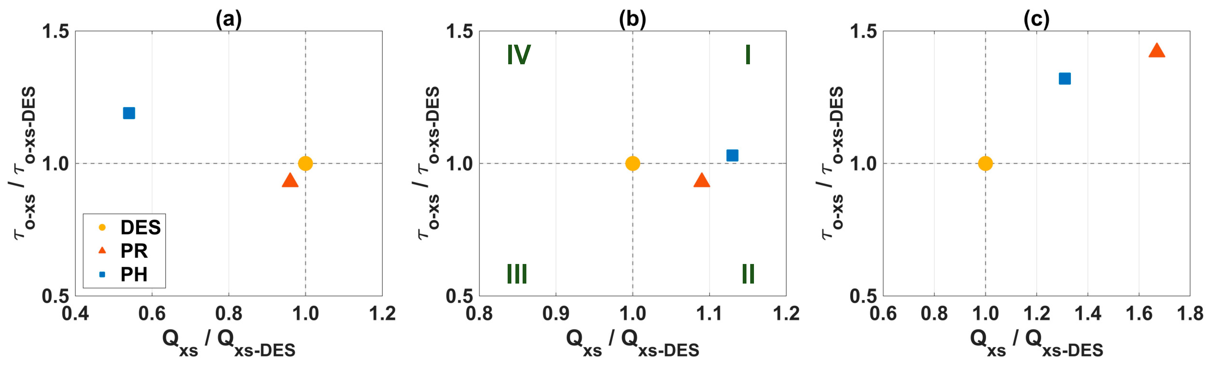
Previous analyses indicated that the applied stresses were affected by the local degree of measured morphodynamic adjustment (Figure 5). If changes associated with bank properties and conditions were not as pronounced, this implied that a given cross-section would experience more or less erosion depending primarily on the trajectory of the adjustment (Figure 7). Physically, BEHI scores (Table 3) did not provide a quantitative understanding of the erodibility phenomenon, neither in terms of resisting (e.g., τc and kd), nor applied (e.g., τo) forces; rather, they only provided a qualitative assessment of how likely a bank was to undergo erosion. In contrast, BSTEM erosion predictions were based on the excess shear stress acting on banks, balancing resisting and applied forces as dictated by cross-sectional geometry, soil properties, and flow characteristics. A process-based representation such as this acknowledged that erodibility was a compound phenomenon, in which highly erodible banks were necessary, but not sufficient, as applied stresses capable of generating erosion were also required. In the BANCS model, the compound phenomenon was considered through erodibility curves that used both BEHI and NBS as predictor variables [25]. However, BEHI scores had also been applied as stand-alone parameters to estimate bank erosion rates (e.g., [23,52,64]).
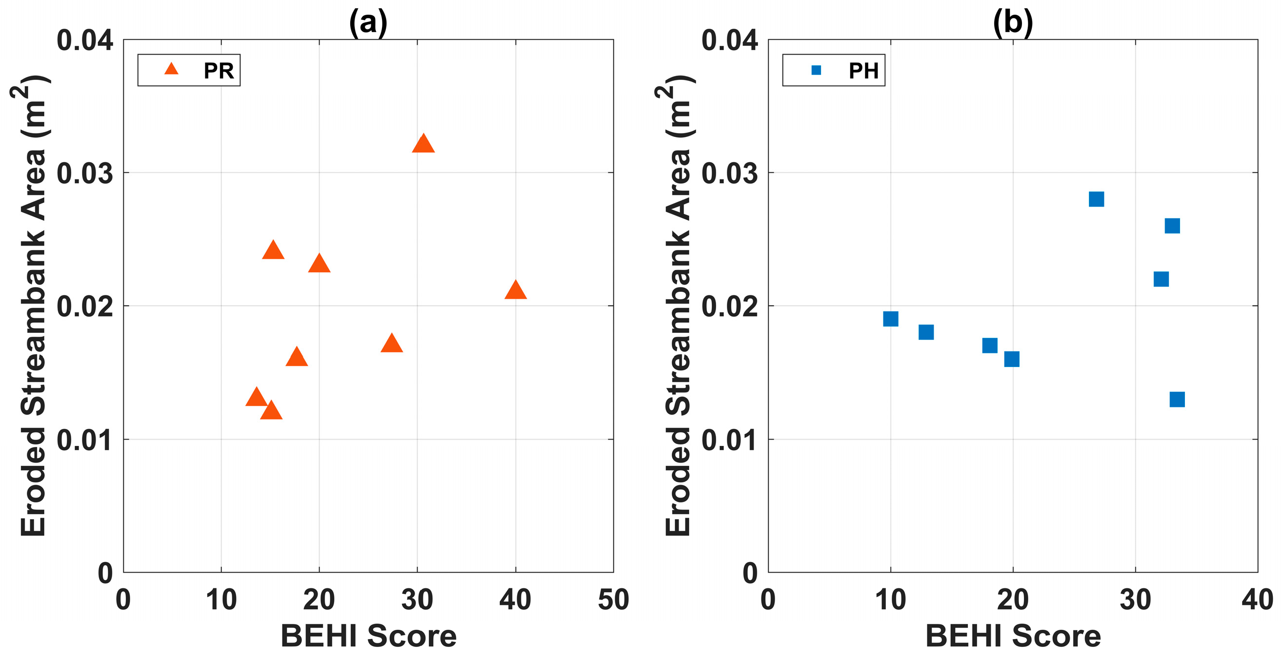
At the local-scale, the Pearson’s correlation coefficient (ρcoeff) [
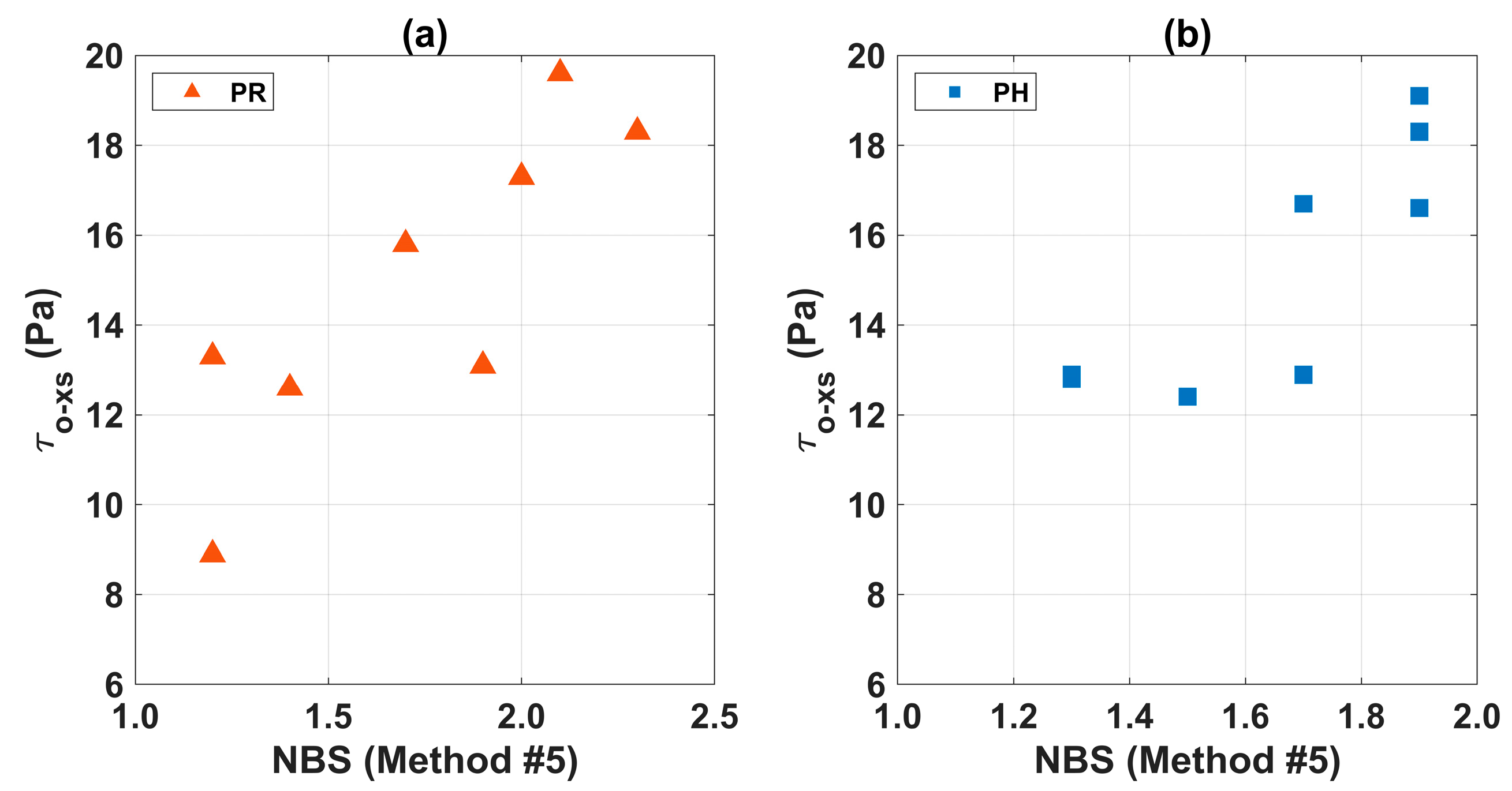
62] was calculated to examine the linear dependence between BSTEM process-based predictions of eroded bank area at each cross-section and form-based BEHI scores for bank erosion potential. These data are shown in Figure 8, where the eroded bank area represented the detached area in the direction perpendicular to the flow normalized by the input duration of flow. Results corresponded to ρcoeff of 0.47 for the PR geometry (Figure 8a) and ρcoeff of 0.29 for the PH geometry (Figure 8b). Statistically, the low values of ρcoeff indicated that the correlation between these variables was not strong, meaning that the eroded bank area computed by BSTEM did not consistently increase with increasing BEHI scores. Results in Figure 8 suggested that BEHI scores were not able to capture the measured morphodynamic adjustments following the severe floods in 2018. Even though the correlation was not strong for the PR geometry with ρcoeff = 0.47, it significantly deteriorated for the PH geometry with ρcoeff = 0.29. This trend suggested that BEHI scores may not have the resolution to accurately describe these types of short-term morphodynamic adjustments.

4.2.2. Volumetric Amount

Volumetric amounts of geomorphic change were calculated based on the predictions from BANCS, BSTEM, HEC-RAS 1D, and HEC-RAS 1D & BSTEM. Results are presented in Table 7 for the DES, PR, and PH geometries. These results corresponded to cumulative volumetric amounts of geomorphic change across the eight cross-sections as dictated by morphodynamic processes included in each modeling approach. Volumetric amounts from BANCS were computed using erosion rates (which were converted into volumes based on bank height and length) from the North Carolina Bank Erodibility Curve [53] that applied BEHI and NBS (Method #5) as predictor variables. BANCS volumetric amounts were given on an annual basis, accounted only for bank erosion, and were based on the evaluated bank (i.e., RB or LB) at the eight cross-sections. Furthermore, it should be noted that BANCS volumetric amounts were computed using NBS Method #5 and could change depending on the applied method (e.g., [14,25,50]). BSTEM volumetric amounts were calculated using eroded bank areas that were converted into volumes based on bank length, as well as dislodged sediment volumes due to bank geotechnical failure. Similar to BANCS predictions, BSTEM volumetric amounts were based on the evaluated bank (i.e., RB or LB) at the eight cross-sections. For HEC-RAS 1D, volumetric amounts were based on predicted changes over entire cross-sections along the study reach, either by accounting only for bed material transport (i.e., HEC-RAS 1D) or by adding the contribution of bank erosion and failure (i.e., HEC-RAS 1D & BSTEM). In contrast to BANCS predictions, volumetric amounts of geomorphic change from BSTEM and HEC-RAS 1D were given on an event basis.
At a local scale, BANCS and BSTEM predictions indicated that a process-based approach to directly account for bank failure increased the volumetric amount by an order of magnitude (Table 7). In the BANCS model, the potential for bank failure was indirectly considered through metrics that included bank height and angle as part of BEHI assessments. The volumetric amount varied from −2.4 m3 to −18.6 m3 for the PR geometry, and from −2.7 m3 to −26.7 m3 for the PH geometry (where the negative sign indicated erosion). Beyond the driving morphodynamic processes, note the different time scales associated with BANCS and BSTEM results. BANCS volumetric amounts were given on an annual basis following the time resolution of the applied bank erodibility curve. In general, as discussed by Bigham et al. [25], available erodibility curves show marked variability in terms of number of sites, years of measurements, and range of discharges that occurred during measurements. Hence, the accuracy of BANCS predictions is closely related to the amount and quality of data that were used to develop a specific curve. For North Carolina, the applied bank erodibility curve was based on measurements at 20 cross-sections distributed across six stream reaches that represented various land uses [53,65]. According to the summary provided in Bigham et al. [25], the measurements corresponded to one year of data with no reported range of discharges. Doll et al. [53] noted this limitation, indicating the need for expanding the North Carolina Bank Erodibility curve by lengthening the monitoring period and increasing the range of discharges experienced during measurements.
Depending on the frequency of measurements, the contribution of severe or rare floods may not be accurately captured by erodibility curves developed from the BANCS methodology. As shown by the PH geometry results, these types of events can have a pronounced impact on the stream’s water conveyance and sediment transport capacity (Figure 7). Similar findings were reported by Dave et al. [66] in the Cedar River, Nebraska, USA, where 29% of the bank retreat experienced over a period of 10 years was caused by a single flood following a dam breach. These observations suggest that predictions from the BANCS model may be more suitable for streams that show limited variability in flow distribution where a single discharge is more representative of reach-averaged conditions, unless data for constructing bank erodibility curves are collected over an extended period and at a higher frequency to capture the contribution of severe or rare floods. BSTEM volumetric amounts, alternatively, can account for the process-based response of streams to individual floods (i.e., event basis), which is fundamental to improve our understanding of how non-stationary climatic conditions affect geomorphic change [67]. In this study, for example, BSTEM results for the PR and PH geometries indicated that a single bankfull flood event had the capacity to generate higher volumetric amounts than those predicted by BANCS on an annual basis (Table 7).
Among process-based models, BSTEM and HEC-RAS 1D predictions indicated that considering bed material transport increased the volumetric amount by two orders of magnitude (Table 7). Based on HEC-RAS 1D, the volumetric amount varied from −18.6 m3 to +1374.2 m3 for the PR geometry, and from −26.7 m3 to +1138.2 m3 for the PH geometry (where the positive sign indicated deposition). The pronounced variation in magnitude showed that bed material transport dominated geomorphic changes along the sand-bed study reach. Additionally, changes in sign denoted a different stream response from erosion (as predicted by BSTEM) to deposition (as predicted by HEC-RAS 1D). Physically, these observations suggested that the stream did not have enough bed material transport capacity. Numerically, they emphasized the need for applying process-based, reach-scale models to analyze streams with highly mobile bed material.
Among reach-scale models, HEC-RAS 1D and HEC-RAS 1D & BSTEM predictions indicated that considering bed material transport coupled with bank erosion and failure produced the highest volumetric amounts of geomorphic change (Table 7). The volumetric amount varied from +1374.2 m3 to +2043.6 m3 for the PR geometry, and from +1138.2 m3 to +1726.7 m3 for the PH geometry. Physically, results suggested that bank retreat led to cross-sectional widening, which in turn led to a reduction in water conveyance and sediment transport capacity, resulting in more pronounced deposition levels. Moreover, feedback effects between bed material transport and bank retreat had a non-linear impact on the magnitude of volumetric amounts of geomorphic change. When comparing HEC-RAS 1D and HEC-RAS 1D & BSTEM predictions, the volumetric amount increased by approximately 50% for both geometries, which represented an increase in volume that was much larger than the stand-alone amount predicted by BSTEM. Numerically, these observations suggested that process-based, reach-scales models that simultaneously account for bed material transport and bank retreat should be used to analyze streams with highly erosional cross-sectional boundaries.
Lastly, for the DES geometry, BSTEM predicted a volumetric amount of −2.6 m3, which was driven by erosion given that no bank was found geotechnically unstable or conditionally stable (i.e., FS > 1.3 along the study reach). Similar to the PR and PH geometries, the volumetric amount increased to −463.3 m3 when accounting for bed material transport (i.e., HEC-RAS 1D) and to −759.9 m3 when adding the contribution of bank retreat (i.e., HEC-RAS 1D & BSTEM). However, as denoted by the negative sign, HEC-RAS 1D and HEC-RAS 1D & BSTEM results showed a different stream response in the case of the DES geometry. Physically, the DES geometry results suggested that initial bed erosion led to incision, localized steeper bottom slopes, and higher and unstable banks, which eventually led to bank failure, widening, and bed deposition. These results emphasized the importance of adequate model selection both, in terms of formulation and scale, to capture dominant morphodynamic processes and improve the quantitative understanding of stream response to restoration efforts.

4.3. Comparison to Measured Post-Restoration Data

To assess the models’ performance, numerical predictions were compared to measured data obtained annually at six-cross-sections as part of the post-restoration monitoring efforts [32]. Consistent with the model-to-model assessments, the comparison focused on the field-based variation of τo and the volumetric amount of geomorphic change. The measured reach-averaged cross-sectional area, channel width, flow depth, and friction slope (Sf) at bankfull conditions are presented in Table 8, where the year 2010 corresponded to the baseline (as-built) monitoring report. Over a period of six years, the response of the study reach was dominated by reductions in cross-sectional area and flow depth. These field measurements indicated that the stream had primarily aggraded, as dictated by feedback effects between bed material transport and bank retreat.
The reach-averaged τo and volumetric amounts were estimated based on the field measurements presented in Table 8. The reach-averaged τo was computed as follows [49]:
τo = ρgRhSf,
where ρ is the density of water, g is the gravitational acceleration, and Rh is the hydraulic radius. Volumetric amounts were calculated based on the difference in cross-sectional area between consecutive monitoring periods and the length of the study reach. The estimated values for both variables are presented in Table 9. In the case of τo, results showed an initial increase in magnitude from 2010 to 2012, followed by a reduction of approximately 30% by 2016, with an overall average magnitude of 17.8 Pa. When compared to process-based modeling predictions, the estimated reach-averaged variation of τo was similar to that predicted by BSTEM, which ranged from 14.8 Pa to 16.7 Pa depending on the geometry. Similar to BSTEM predictions, the estimated field-based τo did not account for the effect of bed material transport dynamics; rather, it was based on erosion and deposition patterns that existed at the time of measurement (i.e., fixed-bed approach). Therefore, the estimated field-based values also represented close to maximum values of τo at bankfull conditions.
Results corresponding to volumetric amounts of geomorphic change indicated that it had significantly fluctuated from 2010 to 2016, showing a threefold increase from 2010 to 2013 and then reducing by approximately 50% by 2016, with an overall average value of +2321.9 m3 (where the positive sign indicated deposition). When compared to modeling predictions, the estimated volumetric amount was similar to that predicted by HEC-RAS 1D & BSTEM, which varied between +1726.7 m3 and +2043.6 m3 for the PR and PH geometries. Reductions in cross-sectional area and flow depth along with increased channel width measured in 2011 (Table 8) suggested that bed erosion and unstable banks could have initially governed the study reach response, causing subsequent widening, reductions in sediment transport capacity, and overall deposition. Albeit available field measurements did not allow for direct comparisons, a similar erosion-driven morphodynamic behavior was predicted by HEC-RAS 1D & BSTEM for the DES geometry. Overall, the comparison between modeling results and measured post-restoration data highlighted the importance of adequate model selection as dictated by the morphodynamic processes and geomorphic conditions that governed stream response.

5. Conclusions

Model-to-model assessments were conducted to quantify the impact of model selection when predicting applied stress and volumetric amounts of geomorphic change in a restored sand-bed stream in North Carolina, USA. Specifically, models that differ in their formulation (form-based vs. process-based) and scale (local-scale vs. reach-scale) were applied, including BEHI, BANCS, BSTEM, and HEC-RAS 1D. Models’ performance was assessed using measured data from six years of post-restoration monitoring reports.
At the reach scale, model selection was dictated by the degree of mobility of the bed material. It was shown that a process-based, reach-scale model, such as HEC-RAS 1D, was needed to accurately analyze streams with fine-grained beds, in which feedback effects between sediment transport and bank retreat are important. Results indicated that failing to account for these feedback effects underpredicted volumetric amounts of geomorphic change by up to three orders of magnitude. In the case of applied stresses, comparisons against measured post-restoration data suggested that fixed-bed approaches, such as BSTEM, rendered a more accurate quantification of maximum values that were experienced for a given cross-sectional geometry. As implemented herein, values of applied shear stress obtained from the quasi-unsteady, mobile-bed HEC-RAS 1D simulations were representative of quasi-equilibrium conditions, which could be attained in practice only if the incoming water discharge was associated with a sufficiently large temporal scale.
At the local scale, model selection was dictated by the dominant mechanism for bank retreat and the variability in flow distribution. It was shown that predictor variables, such as BEHI and NBS (Method #5), used in form-based models, such as BANCS to characterize bank erosion potential and applied stresses, did not fully capture morphodynamic adjustments following severe floods. Results suggested that form-based models such as BANCS may be more suitable for streams with limited flow variability, unless annual bank erodibility curves are constructed with data that accommodate severe or rare floods. Moreover, the application of form-based models such as BANCS rendered the lowest volumetric amounts of geomorphic change, failing to directly account for the contribution of dislodged sediment due to bank geotechnical failure without providing a quantitative measure of applied stresses.
It was shown that process-based models such as BSTEM can be effectively combined with stage-discharge predictor curves as a practical tool to monitor the evolution, infer the trajectory of future changes, and examine the impact of severe floods at the local scale. In addition to providing a quantitative and predictive understanding of the stream’s morphodynamic behavior, the application of process-based, local-scale models, such as BSTEM, did not require a significant amount of additional field data when compared to that already required for form-based models such as BANCS. Moreover, the combination of process-based, local-scale models, such as BSTEM, with stage-discharge predictor curves addressed the limitation that local-scale models did not conserve water discharge, while providing insights on reach-scale morphodynamic behavior.
The application of more advanced process-based models will provide an improved quantification of applied stresses, impacting in turn predicted volumetric amounts of geomorphic change. For example, two-dimensional numerical models (e.g., HEC-RAS 2D [68] and SHR-2D [69]) simulate the variation along the cross-section of depth-averaged applied stresses, whereas three-dimensional models (e.g., [70]) simulate the spatial distribution of applied stresses along the wetted bank. However, the application of these models is still constrained by required extensive parameterization using site-specific data that have not been readily available and simplifying assumptions needed to perform the numerical simulations [69,70]. Moreover, another key factor that may be difficult to parameterize in process-based models is the effect of bank vegetation on applied stresses. For example, Liu et al. [71] showed through a series of flume experiments that turbulence intensity can increase in the main channel and decrease in the bank toe region as bank vegetation density increases. Therefore, the selection and application of process-based models should consider the tradeoff among data requirements, computational costs, prediction uncertainty, and desired accuracy.
The main local and regional factors influencing the results of this study were the stream’s geomorphic characteristics and the climatic features to which the stream is subjected because of its location in the Northern Outer Piedmont ecoregion of the Piedmont physiographic region of North Carolina, USA [72]. Relevant to the models’ application, these factors are important when characterizing the bed and bank material composition and erodibility, as well as the discharge data used to perform the numerical simulations. Importantly, the Jet Erosion Test was applied in this study to measure in-situ bank material erodibility. Alternatively, a number of empirical equations exist that can be used to estimate erodibility parameters based on the bank material composition (e.g., [73]). Moreover, regional climatic features drive daily and seasonal changes in environmental conditions, such as temperature and moisture content, which have been shown to impact the magnitude of soil erodibility parameters [74]. Consideration should be given to these factors when transferring results and findings from this study to other regions.

Author Contributions

Conceptualization, C.C.-B., G.A.F., L.G. and P.R.; methodology, K.K., C.C.-B. and E.D.B.; software, K.K.; validation, K.K. and C.C.-B.; formal analysis, K.K. and C.C.-B.; investigation, K.K. and C.C.-B.; resources, C.C.-B. and P.R.; data curation, K.K. and C.C.-B.; writing—original draft preparation, K.K. and C.C.-B.; writing—review and editing, C.C.-B., G.A.F., L.G., P.R. and E.D.B.; visualization, K.K. and C.C.-B.; supervision, C.C.-B.; project administration, C.C.-B.; funding acquisition, C.C.-B. All authors have read and agreed to the published version of the manuscript.

Funding

This research was funded by the North Carolina Department of Environmental Quality Division of Mitigation Services (DEQ Contract No. 7542) and the USDA National Institute of Food and Agriculture (Hatch Project 1016113).

Institutional Review Board Statement

Not applicable.

Informed Consent Statement

Not applicable.

Data Availability Statement

The data presented in this study are available on request from the corresponding author.

Acknowledgments

The authors would like to acknowledge Casey Haywood (NCDEQ) and Alexis Swanson (NCSU BAE) for their support with field measurements, as well as Kris Bass (Kris Bass Engineering) for his assistance with numerical modeling.

Conflicts of Interest

The authors declare no conflict of interest.

References

  1. Bernhardt, E.S.; Palmer, M.A.; Allan, J.D.; Alexander, G.; Barnas, K.; Brooks, S.; Carr, J.; Clayton, S.; Dahm, C.; Follstad-Shah, J.; et al. Synthesizing U.S. River Restoration Efforts. Science 2005, 308, 636–637. [Google Scholar] [CrossRef] [PubMed]
  2. Wohl, E.; Angermeier, P.L.; Bledsoe, B.; Kondolf, G.M.; MacDonnell, L.; Merritt, D.M.; Palmer, M.A.; Poff, N.L.; Tarboton, D. River restoration. Water Resour. Res. 2005, 41, W10301. [Google Scholar] [CrossRef]
  3. Wohl, E.; Lane, S.N.; Wilcox, A.C. The Science and Practice of River Restoration. Water Resour. Res. 2015, 51, 5974–5997. [Google Scholar] [CrossRef] [Green Version]
  4. Enlow, H.K.; Fox, G.A.; Boyer, T.A.; Stoecker, A.; Storm, D.E.; Starks, P.; Guertault, L. A Modeling Framework for Evaluating Streambank Stabilization Practices for Reach-Scale Sediment Reduction. Environ. Model. Softw. 2018, 100, 201–212. [Google Scholar] [CrossRef]
  5. Bigham, K.A. Streambank Stabilization Design, Research, and Monitoring: The Current State and Future Needs. Trans. ASABE 2020, 63, 351–387. [Google Scholar] [CrossRef]
  6. Russell, M.V.; Mittelstet, A.R.; Joeckel, R.M.; Korus, J.T.; Castro-Bolinaga, C.F. Impact of Bank Stabilization Structures on Upstream and Downstream Bank Mobilization at Cedar River, Nebraska. Trans. ASABE 2021, 64, 1555–1567. [Google Scholar] [CrossRef]
  7. Miller, J.R.; Kochel, R.C. Assessment of Channel Dynamics, In-Stream Structures and Post-Project Channel Adjustments in North Carolina and its Implications to Effective Stream Restoration. Environ. Earth Sci. 2010, 59, 1681–1692. [Google Scholar] [CrossRef]
  8. Castro-Bolinaga, C.F.; Fox, G.A. Streambank Erosion: Advances in Monitoring, Modeling and Management. Water 2018, 10, 1346. [Google Scholar] [CrossRef] [Green Version]
  9. Papangelakis, E.; MacVicar, B. Process-based Assessment of Success and Failure in a Constructed Riffle-Pool River Restoration Project. River Res Applic. 2020, 36, 1222–1241. [Google Scholar] [CrossRef]
  10. Mal, S.; Singh, R.B.; Huggel, C.; Grover, A. Introducing Linkages between Climate Change, Extreme Events, and Disaster Risk Reduction. In Climate Change, Extreme Events and Disaster Risk Reduction, Towards Sustainable Development Goals; Mal, S., Singh, R.B., Huggel, C., Eds.; Springer: Cham, Switzerland, 2018; pp. 1–14. [Google Scholar] [CrossRef]
  11. Fox, G.A. Process-Based Design Strengthens the Analysis of Stream and Floodplain Systems under a Changing Climate. Trans. ASABE 2019, 62, 1735–1742. [Google Scholar] [CrossRef]
  12. Syvitski, J.; Ángel, J.R.; Saito, Y.; Overeem, I.; Vörösmarty, C.J.; Wang, H.; Olago, D. Earth’s sediment cycle during the Anthropocene. Nat. Rev. Earth Environ. 2022, 3, 179–196. [Google Scholar] [CrossRef]
  13. Jacobson, R.B.; Berkley, J. Conceptualizing and Communicating Ecological River Restoration. In Stream Restoration in Dynamic Fluvial Systems: Scientific Approaches, Analyses, and Tools; Simon, A., Bennett, S.J., Castro, J.M., Eds.; John Wiley & Sons: Hoboken, NJ, USA, 2011; Volume 194, pp. 9–27. [Google Scholar] [CrossRef]
  14. Rosgen, D.L. Watershed Assessment of River Stability and Sediment Supply (WARSSS); Wildland Hydrology: Fort Collins, CO, USA, 2009. [Google Scholar]
  15. USDA-ARS. Bank Stability and Toe Erosion Model (BSTEM); U.S. Department of Agriculture, Agricultural Research Service: Washington, DC, USA, 2023. Available online: https://www.ars.usda.gov/southeast-area/oxford-ms/national-sedimentation-laboratory/watershed-physical-processes-research/research/bstem/overview/ (accessed on 8 March 2023).
  16. Brunner, G.W. HEC-RAS River Analysis System User’s Manual, Version 5.0; U.S. Army Corps of Engineers, Institute for Water Resources, Hydrologic Engineering Center: Davis, CA, USA, 2016.
  17. USDA. Stream Restoration Design, National Engineering Handbook 654; U.S. Department of Agriculture, Natural Resources Conservation Service: Washington, DC, USA, 2007. Available online: https://directives.sc.egov.usda.gov/viewerFS.aspx?hid=21433 (accessed on 8 March 2023).
  18. Harman, W.; Starr, R.; Carter, M.; Tweedy, K.; Clemmons, M.; Suggs, K.; Miller, C. A Function-Based Framework for Stream Assessment & Restoration Projects; U.S. Environmental Protection Agency, Office of Wetlands, Oceans, and Watersheds: Washington, DC, USA, 2012; EPA 843-K-12-006.
  19. Yochum, S.E. Guidance for Stream Restoration and Rehabilitation, Technical Note TN-102.4; U.S. Department of Agriculture, Forest Service, National Stream & Aquatic Ecology Center: Fort Collins, CO, USA, 2018.
  20. Smith, S.M.; Prestegaard, K.L. Hydraulic Performance of a Morphology-Based Stream Channel Design. Water Resour. Res. 2005, 41, W11413. [Google Scholar] [CrossRef] [Green Version]
  21. Simon, A.; Doyle, M.; Kondolf, M.; Shields, F.D., Jr.; Rhoads, B.; McPhillips, M. Critical Evaluation of How the Rosgen Classification and Associated “Natural Channel Design” Methods Fail to Integrate and Quantify Fluvial Processes and Channel Response. JAWRA J. Am. Water Resour. Assoc. 2007, 43, 1117–1131. [Google Scholar] [CrossRef]
  22. Roper, B.B.; Buffington, J.M.; Archer, E.; Moyer, C.; Ward, M. The Role of Observer Variation in Determining Rosgen Stream Types in Northeastern Oregon Mountain Streams. JAWRA J. Am. Water Resour. Assoc. 2008, 44, 417–427. [Google Scholar] [CrossRef]
  23. Ghosh, K.G.; Pal, S.; Mukhopadhyay, S. Validation of BANCS Model for Assessing Stream Bank Erosion Hazard Potential (SBEHP) in Bakreshwar River of Rarh Region, Eastern India. Model. Earth Syst. Environ. 2016, 2, 95. [Google Scholar] [CrossRef] [Green Version]
  24. McMillan, M.; Liebens, J.; Metcalf, C. Evaluating the BANCS Streambank Erosion Framework on the Northern Gulf of Mexico Coastal Plain. JAWRA J. Am. Water Resour. Assoc. 2017, 53, 1393–1408. [Google Scholar] [CrossRef]
  25. Bigham, K.A.; Moore, T.L.; Vogel, J.R.; Keane, T.D. Repeatability, Sensitivity, and Uncertainty Analyses of the BANCS Model Developed to Predict Annual Streambank Erosion Rates. JAWRA J. Am. Water Resour. Assoc. 2018, 54, 423–439. [Google Scholar] [CrossRef]
  26. Shields, F.D.; Copeland, R.R.; Klingeman, P.C.; Doyle, M.W.; Simon, A. Design for Stream Restoration. J. Hydraul. Eng. 2003, 129, 575–584. [Google Scholar] [CrossRef]
  27. Lammers, R.W.; Bledsoe, B.P.; Langendoen, E.J. Uncertainty and sensitivity in a bank stability model: Implications for estimating phosphorus loading. Earth Surf. Process. Landf. 2017, 42, 612–623. [Google Scholar] [CrossRef] [Green Version]
  28. Simon, A.; Pollen-Bankhead, N.; Thomas, R.E. Development and Application of a Deterministic Bank Stability and Toe Erosion Model for Stream Restoration. In Stream Restoration in Dynamic Fluvial Systems: Scientific Approaches, Analyses, and Tools; Simon, A., Bennett, S.J., Castro, J.M., Eds.; John Wiley & Sons: Hoboken, NJ, USA, 2011; Volume 194, pp. 453–474. [Google Scholar] [CrossRef]
  29. Papanicolaou, A.N.; Elhakeem, M.; Hilldale, R. Secondary Current Effects on Cohesive River Bank Erosion. Water Resour. Res. 2007, 43, W12418. [Google Scholar] [CrossRef]
  30. Tullos, D.; Baker, D.W.; Crowe Curran, J.; Schwar, M.; Schwartz, J. Enhancing resilience of river restoration design in systems undergoing change. J. Hydraul. Eng. 2021, 147, 03121001. [Google Scholar] [CrossRef]
  31. USGS. StreamStats: Streamflow Statistics and Spatial Analysis Tools for Water-Resources Applications; U.S. Geological Survey: Reston, VA, USA, 2023. Available online: https://streamstats.usgs.gov/ss/ (accessed on 8 March 2023).
  32. NCDEQ-DMS. Paschal Golf Course (Richland Creek) Stream Restoration Monitoring Report, Monitoring Year 05; KCI Associates of North Carolina: Raleigh, NC, USA, 2016. [Google Scholar]
  33. NCDEQ-DMS. DMS Project Documents Table; Division of Mitigation Services, North Carolina Department of Environmental Quality: Raleigh, NC, USA, 2023. Available online: https://deq.nc.gov/about/divisions/mitigation-services/dms-project-documents-table (accessed on 8 March 2023).
  34. Kassa, K.H. A Multi-Scale Modeling Approach to Examine Bank Erosion and Sediment Transport in Stream Restoration: A Case Study in the North Carolina Piedmont Region. Master’s Thesis, North Carolina State University, Raleigh, NC, USA, 2019. Available online: http://www.lib.ncsu.edu/resolver/1840.20/36717 (accessed on 8 March 2023).
  35. Hanson, G.J. Surface erodibility of earthen channel at high stresses: Part II. Developing an in-situ testing device. Trans. ASAE 1990, 33, 132–137. [Google Scholar] [CrossRef]
  36. Hanson, G.J. Development of a jet index to characterize erosion resistance of soils in earthen spillways. Trans. ASAE 1991, 34, 2015–2020. [Google Scholar] [CrossRef]
  37. Fox, G.A.; Guertault, L.; Castro-Bolinaga, C.F.; Allen, P.; Bigham, K.A.; Bonelli, S.; Hunt, S.L.; Kassa, K.; Langendoen, E.J.; Porter, E.; et al. Perspectives on the Jet Erosion Test (JET): Lessons Learned, Challenges and Opportunities in Quantifying Cohesive Soil Erodibility. J. ASABE 2022, 65, 197–207. [Google Scholar] [CrossRef]
  38. Al-Madhhachi, A.-T.; Hanson, G.J.; Fox, G.A.; Tyagi, A.K.; Bulut, R. Measuring soil erodibility using a laboratory “mini” JET. Trans. ASABE 2013, 56, 901–910. [Google Scholar] [CrossRef]
  39. Hanson, G.J.; Cook, K.R. Development of Excess Shear Stress Parameters for Circular Jet Testing. In ASAE Paper No. 972227, Proceedings of the ASAE Meeting, Minneapolis, MN, USA, 10–14 August 1997; ASAE: St. Joseph, MI, USA, 1997. [Google Scholar]
  40. Hanson, G.J.; Cook, K.R. Apparatus, Test Procedures, and Analytical Methods to Measure Soul Erodibility in Situ. Appl. Eng. Agric. 2004, 20, 455–462. [Google Scholar] [CrossRef]
  41. Daly, E.R.; Fox, G.A.; Miller, R.B.; Al-Madhhachi, A.S.T. A scour depth approach for deriving erodibility parameters from jet erosion tests. Trans. ASABE 2013, 56, 1343–1351. [Google Scholar] [CrossRef]
  42. Simon, A.; Thomas, R.E.; Klimetz, L. Comparison and Experiences with Field Techniques to Measure Critical Shear Stress and Erodibility of Cohesive Deposits. In Proceedings of the 2nd Joint Federal Interagency Conference, Las Vegas, NV, USA, 27 June–1 July 2010. [Google Scholar]
  43. ASCE. Sedimentation Engineering Manual: Processes, Measurements, Modeling, and Practice, ASCE Manuals and Reports on Engineering Practice No. 110; Garcia, M.H., Ed.; American Society of Civil Engineers: Reston, VA, USA, 2008. [Google Scholar]
  44. Hanson, G.J.; Simon, A. Erodibility of cohesive streambeds in the loess area of the midwestern USA. Hydrol. Process. 2001, 15, 23–38. [Google Scholar] [CrossRef]
  45. Doll, B.A.; Wise-Frederick, D.E.; Buckner, C.M.; Wilkerson, S.D.; Harman, W.A.; Smith, R.E.; Spooner, J. Hydraulic Geometry Relationships for Urban Streams Throughout the Piedmont of North Carolina. JAWRA J. Am. Water Resour. Assoc. 2002, 38, 641–651. [Google Scholar] [CrossRef]
  46. Sholtes, J.S.; Bledsoe, B.P. Half-yield discharge: Process-based predictor of bankfull discharge. J. Hydraul. Eng. 2016, 142, 04016017. [Google Scholar] [CrossRef] [Green Version]
  47. Brownlie, W.R. Flow depth in sand-bed channels. J. Hydraul. Eng. 1983, 109, 959–990. [Google Scholar] [CrossRef]
  48. Castro-Bolinaga, C.F.; Diplas, P. Hydraulic Modeling of Extreme Hydrologic Events: Case study in Southern Virginia. J. Hydraul. Eng. 2014, 140, 05014007. [Google Scholar] [CrossRef]
  49. Chang, H.H. Fluvial Processes in River Engineering, 1st ed.; Wiley: New York, NY, USA, 1988. [Google Scholar]
  50. Rosgen, D.L.; Keane, T.D.; Geenen, D. Discussion “Evaluating the BANCS Streambank Erosion Framework on the Northern Gulf of Mexico Coastal Plain” by Mitchell McMillan, Johan Liebens, and Chris Metcalf. JAWRA J. Am. Water Resour. Assoc. 2019, 55, 274–280. [Google Scholar] [CrossRef]
  51. Kwan, H.; Swanson, S. Prediction of annual streambank erosion for Sequoia National Forest, California. JAWRA J. Am. Water Resour. Assoc. 2014, 50, 1439–1447. [Google Scholar] [CrossRef]
  52. Allmanová, Z.; Vlčková, M.; Jankovský, M.; Allman, M.; Merganič, J. How can stream bank erosion be predicted on small water courses? Verification of BANCS model on the Kubrica watershed. Int. J. Sediment Res. 2021, 36, 419–429. [Google Scholar] [CrossRef]
  53. Doll, B.A.; Grabow, G.L.; Hall, K.R.; Halley, J.; Harman, W.A.; Jennings, G.D.; Wise, D.E. Stream Restoration: A Natural Channel Design Handbook; North Carolina Stream Restoration Institute and North Carolina Sea Grant: Raleigh, NC, USA, 2003; Available online: https://www.bae.ncsu.edu/extension/srp/technical-resources/ (accessed on 8 March 2023).
  54. Midgley, T.L.; Fox, G.A.; Heeren, D.M. Evaluation of the bank stability and toe erosion model (BSTEM) for predicting lateral retreat on composite streambanks. Geomorphology 2012, 145, 107–114. [Google Scholar] [CrossRef] [Green Version]
  55. Simon, A.; Curini, A.; Darby, S.E.; Langendoen, E.J. Bank and Near-Bank Processes in an Incised Channel. Geomorphology 2000, 35, 193–217. [Google Scholar] [CrossRef]
  56. Klavon, K.; Fox, G.; Guertault, L.; Langendoen, E.; Enlow, H.; Miller, R.; Khanal, A. Evaluating a process-based model for use in streambank stabilization: Insights on the Bank Stability and Toe Erosion Model (BSTEM). Earth Surf. Process. Landf. 2017, 42, 191–213. [Google Scholar] [CrossRef]
  57. CEIWR-HEC. HEC-RAS USDA-ARS Bank Stability & Toe Erosion Model (BSTEM), Technical Reference & User’s Manual; U.S. Army Corps of Engineers, Institute for Water Resources, Hydrologic Engineering Center (HEC): Davis, CA, USA, 2015. [Google Scholar]
  58. Chow, V.T. Open-Channel Hydraulics, 1st ed.; McGraw-Hill: New York, NY, USA, 1959. [Google Scholar]
  59. Yang, C.T. Incipient Motion and Sediment Transport. Journal of the Hydraulics Division. J. Hydraul. Div. 1973, 99, 1679–1704. [Google Scholar] [CrossRef]
  60. Yang, C.T. Unit stream power equation for gravel. J. Hydraul. Eng. 1984, 110, 1783–1797. [Google Scholar] [CrossRef]
  61. Thomas, W.A. Mathematical modeling of sediment movement. In Gravel Bed Rivers; Hey, R.D., Bathurst, J.C., Thorne, C.R., Eds.; John Wiley & Sons: Hoboken, NJ, USA, 1982; pp. 487–508. [Google Scholar]
  62. Maity, R. Statistical Methods in Hydrology and Hydroclimatology; Springer Nature: Singapore, 2018. [Google Scholar]
  63. Davidson, S.L.; Eaton, B.C. Beyond regime: A stochastic model of floods, bank erosion, and channel migration. Water Resour. Res. 2018, 54, 6282–6298. [Google Scholar] [CrossRef]
  64. Dick, B.M.; Hey, R.; Peralta, P.; Jewell, I.; Simon, P.; Peszlen, I. Estimating Annual Riverbank Erosion Rates—A Dendrogeomorphic Method. River Res. Applic. 2014, 30, 845–856. [Google Scholar] [CrossRef]
  65. Jennings, G.D.; Harman, W.A. Measurement and Stabilization of Streambank Erosion in North Carolina. In Soil Erosion Research, Proceedings of the 21st Century, Proceedings of the International Symposium, Honolulu, HI, USA, 3–5 January 2001; Ascough, J.C., Flanagan, D.C., Eds.; ASAE: St. Joseph, MI, USA, 2001; pp. 537–540. [Google Scholar] [CrossRef]
  66. Dave, N.; Mittelstet, A.; Korus, J.; Waszgis, M. Impact of an Extreme Flood Event on Streambank Retreat: Cedar River, Nebraska, USA. JAWRA J. Am. Water Resour. Assoc. 2020, 56, 528–541. [Google Scholar] [CrossRef]
  67. NASEM. A Vision for NSF Earth Sciences 2020-2030: Earth in Time; National Academies of Sciences, Engineering, and Medicine (NASEM); The National Academies Press: Washington, DC, USA, 2020. [Google Scholar]
  68. USACE. HEC-RAS 2D User’s Manual, Version 6.3. U.S. Army Corps of Engineers, Hydrologic Engineering, Center, 2023. Available online: https://www.hec.usace.army.mil/confluence/rasdocs/r2dum/latest (accessed on 31 March 2023).
  69. Lai, Y.G. Modeling stream bank erosion: Practical stream results and future needs. Water 2017, 9, 950. [Google Scholar] [CrossRef] [Green Version]
  70. Khosronejad, A.; Limaye, A.B.; Zhang, Z.; Kang, S.; Yang, X.; Sotiropoulos, F. On the Morphodynamics of a Wide Class of Large-Scale Meandering Rivers: Insights Gained by Coupling LES with Sediment-Dynamics. J. Adv. Model. Earth Syst. 2023, 15, e2022MS003257. [Google Scholar] [CrossRef]
  71. Liu, D.; Valyrakis, M.; Williams, R. Flow hydrodynamics across open channel flows with riparian zones: Implications for riverbank stability. Water 2017, 9, 720. [Google Scholar] [CrossRef] [Green Version]
  72. NCCO. About North Carolina’s Climate. North Carolina Climate Office. 2023. Available online: https://climate.ncsu.edu/learn/about-our-climate/ (accessed on 31 March 2023).
  73. Mahalder, B.; Schwartz, J.S.; Palomino, A.M.; Zirkle, J. Relationships between physical-geochemical soil properties and erodibility of streambanks among different physiographic provinces of Tennessee, USA. Earth Surf. Process. Landf. 2018, 43, 401–416. [Google Scholar] [CrossRef]
  74. Hoomehr, S.; Akinola, A.I.; Wynn-Thompson, T.; Garnand, W.; Eick, M.J. Water temperature, pH, and road salt impacts on the fluvial erosion of cohesive streambanks. Water 2018, 10, 302. [Google Scholar] [CrossRef] [Green Version]
Figure 1. Restored reach of Richland Creek located within the Neuse River basin (USGS Hydrologic Unit 03020201) in the Northern Outer Piedmont ecoregion of the Piedmont physiographic region of North Carolina, USA. Chosen cross-sections (XS) are shown, indicating the banks that were evaluated using local-scale models as right-bank (RB) or left-bank (LB).
Water 15 01448 g001
Figure 2. Comparison among the Design (DES), Post-Restoration (PR), and Post-Hurricane (PH) geometries at cross-sections (a) XS #4, (b) XS #7, and (c) XS #8.
Water 15 01448 g002
Figure 3. Stage-discharge predictor curves developed for cross-sections XS #4, XS #7, and XS #8 following the methodology proposed by Brownlie [47] for sand-bed channels.
Water 15 01448 g003
Figure 4. Model-to-model assessments conducted for quantifying the impact of model selection when predicting applied stresses and volumetric amounts of geomorphic change.
Water 15 01448 g004
Figure 5. Streamwise variation of τo at each cross-section (τo-xs) normalized by the reach-averaged τo (τo-reach) for the Design (DES), Post-Restoration (PR), and Post-Hurricane (PH) geometries as predicted by (a) BSTEM, (b) HEC-RAS 1D, and (c) HEC-RAS 1D & BSTEM.
Water 15 01448 g005
Figure 6. Correlation between BSTEM process-based predictions of τo at each cross-section (τo-xs) and NBS (Method #5) form-based parameterizations of τo for the (a) Post-Restoration (PR) and (b) Post-Hurricane (PH) geometries. Ratings for NBS (Method #5) are: Very Low (<1.0); Low (1.0–1.5); Moderate (1.5–1.8); High (1.8–2.5); Very High (2.5–3.0); and Extreme (<3.0) [14].
Water 15 01448 g006
Figure 7. Values of Qxs and τo-xs for the Post-Restoration (PR) and Post-Hurricane (PH) geometries normalized by those corresponding to the Design (DES) geometry (Qxs-DES and τo-xs-DES) for (a) XS #4, (b) XS #7, and (c) XS #8. Quadrant Descriptions: I—widening with bed erosion and bank retreat; II—widening with bed deposition; III—narrowing with bed deposition; and IV—incision with bed erosion and bank retreat.
Water 15 01448 g007
Figure 8. Correlation between BSTEM process-based predictions of eroded bank area at each cross-section and form-based BEHI scores for bank erosion potential for the (a) Post-Restoration (PR) and (b) Post-Hurricane (PH) geometries. Ratings for BEHI Scores are: Very Low (5–9.5); Low (10–19.5); Moderate (20–29.5); High (30–39.5); Very High (40–45); and Extreme (46–50) [14].
Water 15 01448 g008
Table 1. Median grain size (d50) and classification of the bed material at the chosen cross-section.
XSd50 (mm)Classification 1
12.15Very fine gravel
21.60Very coarse sand
31.60Very coarse sand
42.40Very fine gravel
52.15Very fine gravel
61.60Very coarse sand
72.00Very coarse sand to very fine gravel
82.40Very fine gravel
1 ACSE Sedimentation Engineering Manual [43].
Table 2. Median grain size (d50), classification, and JET-derived erodibility parameters τc and kd of the bank material at the chosen cross-sections.
XSSided50 (mm)Classification 1τc (Pa) 2kd (cm3/N·s) 2
1LB0.320Medium sand0.145.82
2RB0.350Medium sand2.188.89
3LB0.300Medium sand3.295.68
4RB0.125Very fine to fine sand0.144.72
5LB0.125Very fine to fine sand0.154.65
6RB0.062Coarse silt to very fine sand7.362.60
7RB0.100Very fine sand0.018.60
8LB0.500Medium to coarse sand0.814.69
1 ACSE Sedimentation Engineering Manual [43]; 2 Blaisdell Solution Methodology.
Table 3. Bank Erosion Hazard Index (BEHI) scores and ratings at the chosen cross-section for the Post-Restoration (PR) and Post-Hurricane (PH) geometries.
XSSidePRPH
ScoreRatingScoreRating
1LB15.1Low12.9Low
2RB17.7Low18.1Low
3LB13.6Low19.9Moderate
4RB40.0Very High32.1High
5LB27.4Moderate33.4High
6RB15.3Low10.0Low
7RB20.0Moderate26.8Moderate
8LB30.6High33.0High
Table 4. Near-bank stress (NBS) ratings at the chosen cross-section for the Post-Restoration (PR) and Post-Hurricane (PH) geometries.
XSSidePRPH
Ratio 1RatingRatio 1Rating
1LB1.4Low1.3Low
2RB1.2Low1.3Low
3LB1.2Low1.5Low
4RB1.9High1.7Moderate
5LB2.3High1.9High
6RB1.7Moderate1.7Moderate
7RB2.0High1.9High
8LB2.1High1.9High
1 Method #5—ratio of near-bank maximum depth to bankfull mean depth.
Table 5. Reach-averaged values of τo (τo-reach) for the Design (DES), Post-Restoration (PR), and Post-Hurricane (PH) geometries as predicted by BSTEM, HEC-RAS 1D, and HEC-RAS 1D & BSTEM.
Geometryτo-reach (Pa)
BSTEMHEC-RAS 1DHEC-RAS 1D & BSTEM
DES16.73.33.3
PR14.85.85.8
PH15.25.04.6
Table 6. Estimated proxy discharge for bankfull conditions (Qxs) and BSTEM process-based predictions of τo (τo-xs) at cross-sections XS #4, XS #7, and XS #8 for the Design (DES), Post-Restoration (PR), and Post-Hurricane (PH) geometries.
XSDESPRPH
τo-xs (Pa)Qxs (m3/s)τo-xs (Pa)Qxs (m3/s)τo-xs (Pa)Qxs (m3/s)
414.012.513.112.016.76.8
718.610.817.311.719.112.2
813.914.319.623.818.318.7
Table 7. Volumetric amounts of geomorphic change for the Design (DES), Post-Restoration (PR), and Post-Hurricane (PH) geometries based on predictions from BANCS, BSTEM, HEC-RAS 1D, and HEC-RAS 1D & BSTEM.
GeometryVolumetric Amounts (m3)
BANCS 1BSTEM 2HEC-RAS 1D 2HEC-RAS 1D & BSTEM 2
Bank ErosionBank Erosion and FailureBed Material TransportBed Material Transport; Bank Erosion and Failure
DESn/a−2.6−463.3−759.9
PR−2.4−18.6+1374.2+2043.6
PH−2.7−26.7+1138.2+1726.7
1 Annual basis; 2 Event basis; “+” Indicates deposition; “−” Indicates erosion.
Table 8. Reach-averaged cross-sectional area, channel width, flow depth, and friction slope (Sf) at bankfull conditions obtained from post-restoration monitoring reports [32].
YearReach-Averaged Bankfull Variables
Area (m2)Width (m)Depth (m)Sf (m/m)
20108.239.831.210.0027
20118.0010.140.790.0031
20127.528.921.340.0031
20136.839.910.710.0030
20146.469.660.690.0030
20166.099.091.160.0027
Table 9. Estimated values of the reach-averaged τo (τo-reach) and volumetric amounts of geomorphic change based on field observations from post-restoration monitoring reports.
Yearτo-reach (Pa)Volumetric Amounts (m3)
201017.8-
201120.5+1235.3
201219.5+2609.1
201317.9+3786.5
201417.4+1992.8
201613.9+1985.6
Disclaimer/Publisher’s Note: The statements, opinions and data contained in all publications are solely those of the individual author(s) and contributor(s) and not of MDPI and/or the editor(s). MDPI and/or the editor(s) disclaim responsibility for any injury to people or property resulting from any ideas, methods, instructions or products referred to in the content.

