
Determination of Runoff Curve Numbers for the Growing Season Based on the Rainfall–Runoff Relationship from Small Watersheds in the Middle Mountainous Area of Romania
 , and
, and
Abstract
:1. Introduction
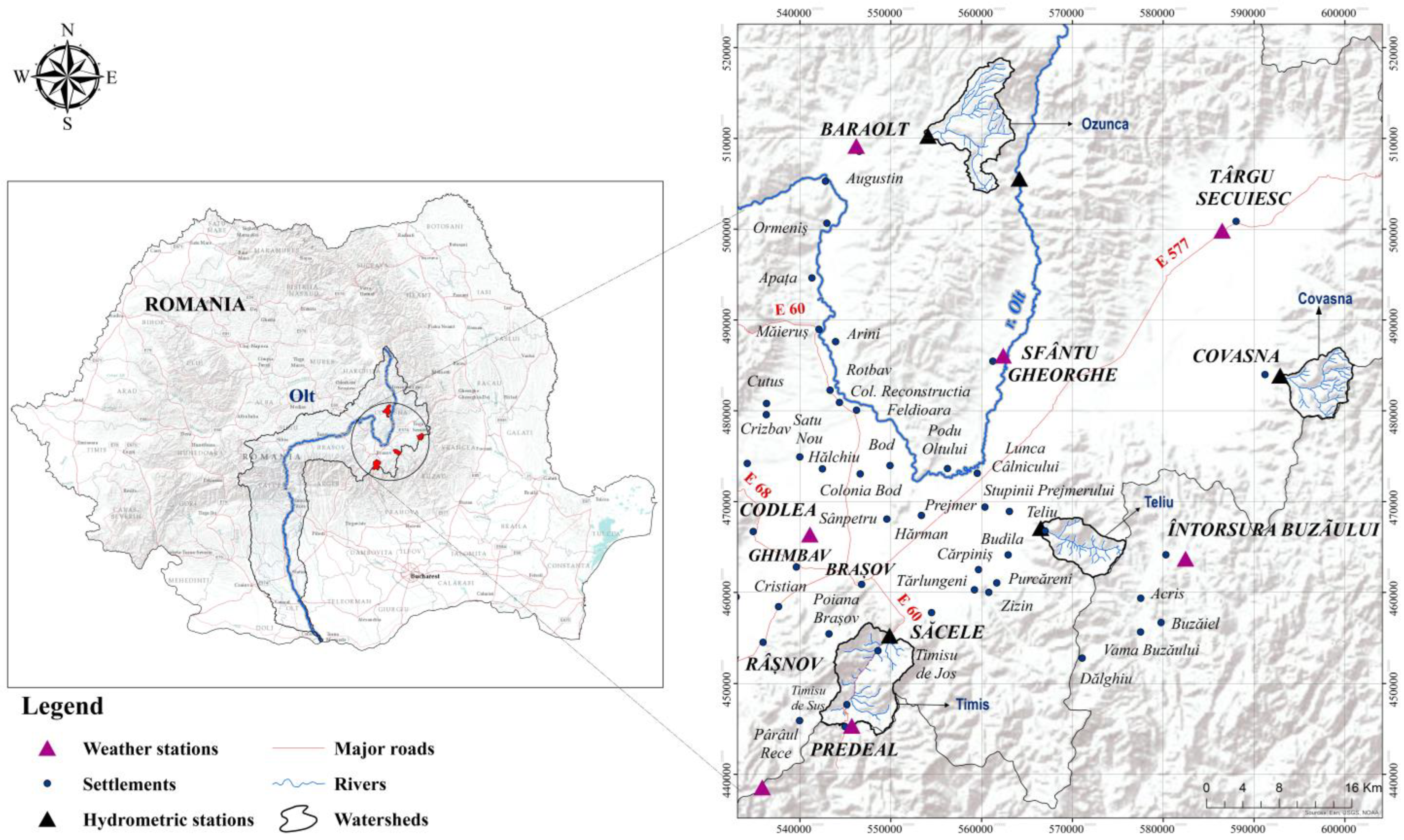
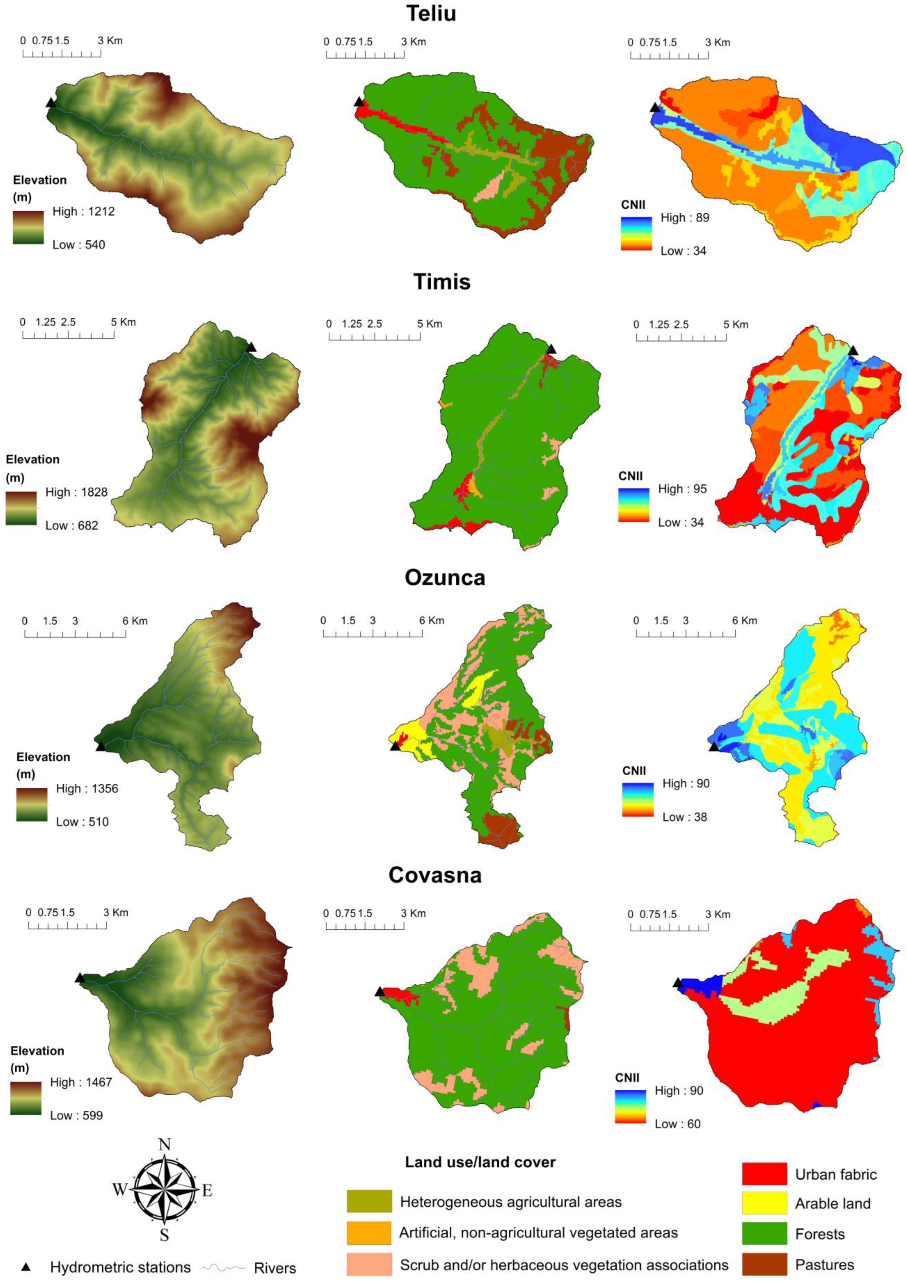
2. Study Area
3. Data and Methodology
3.1. Data
- -
- historical daily records gathered from April to October were selected, when the watersheds are predominantly rain-dominated;
- -
- -
- partial data pairs were manually removed (e.g., only Q data with missing or inconsistent P data, such as in the case of records from 1993 for the Teliu hydrometric station).
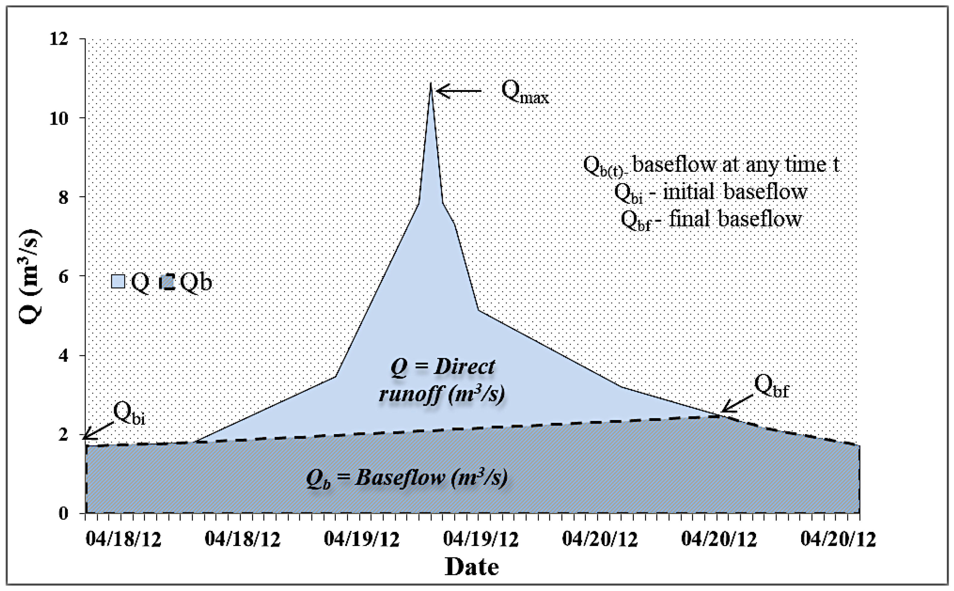
3.2. NRCS-CN Method
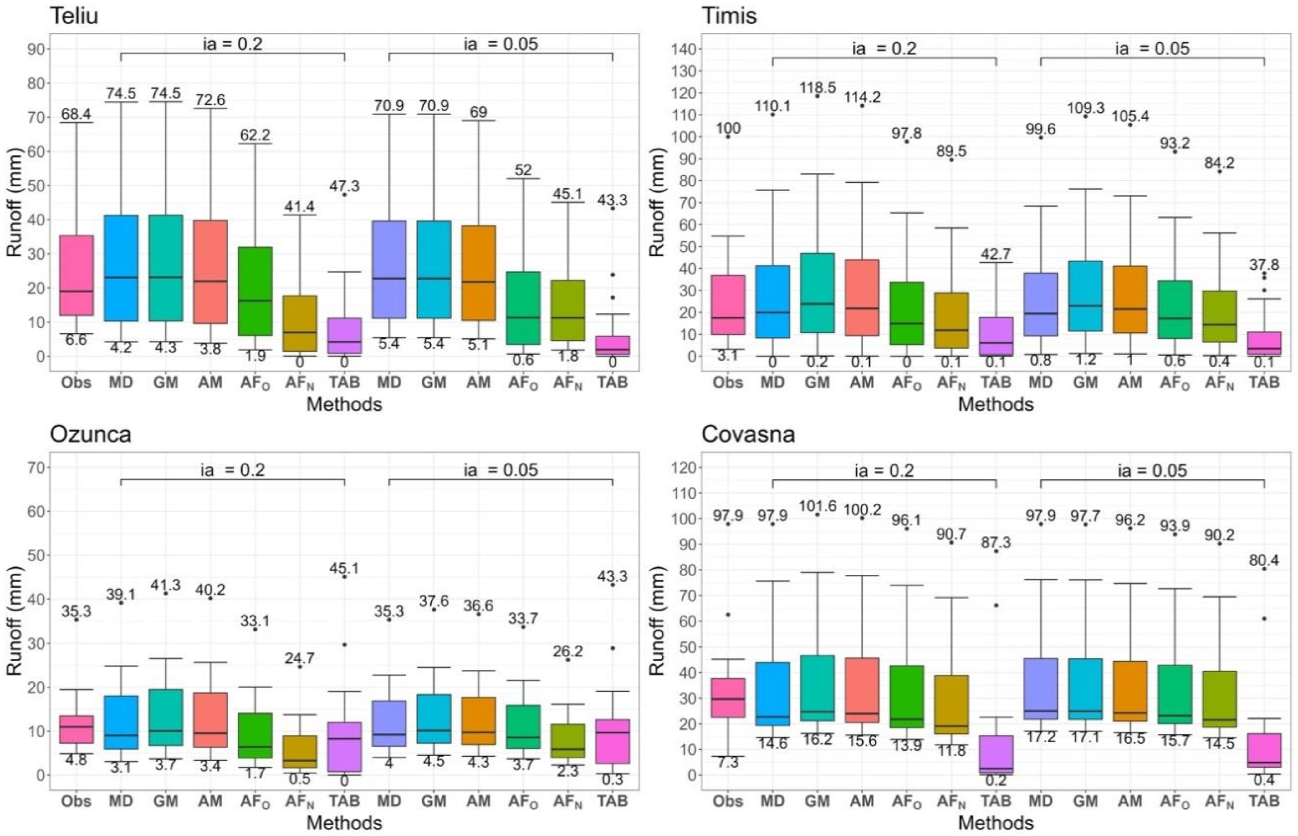
3.3. CN Determination Methods
3.3.1. Tabulated CN Method (TAB; CN Values Selected from NRCS Tables)
3.3.2. Median CN Method (MD)
3.3.3. Geometric Mean CN Method (GM)
3.3.4. Arithmetic Mean CN Method (AM)
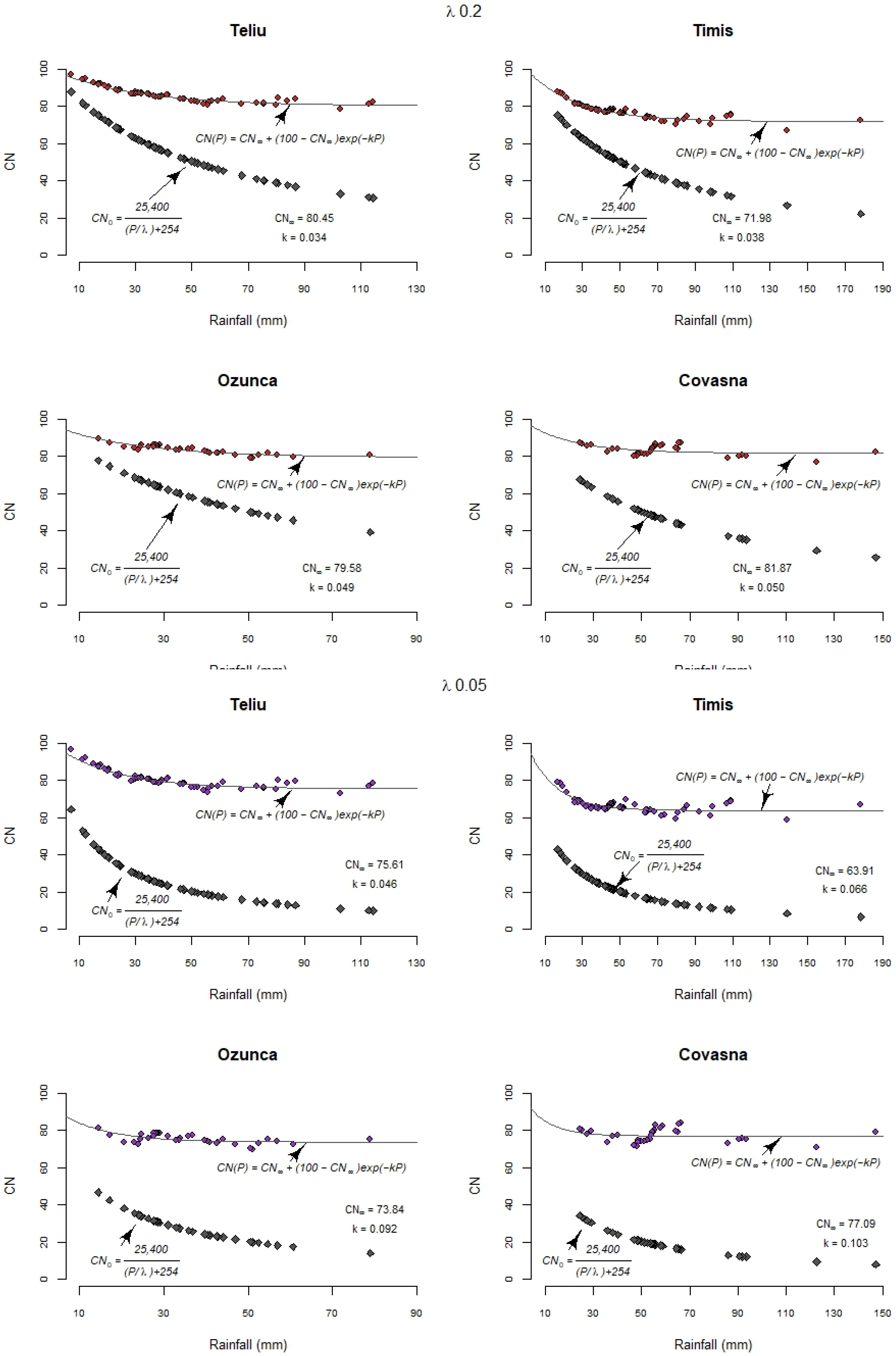
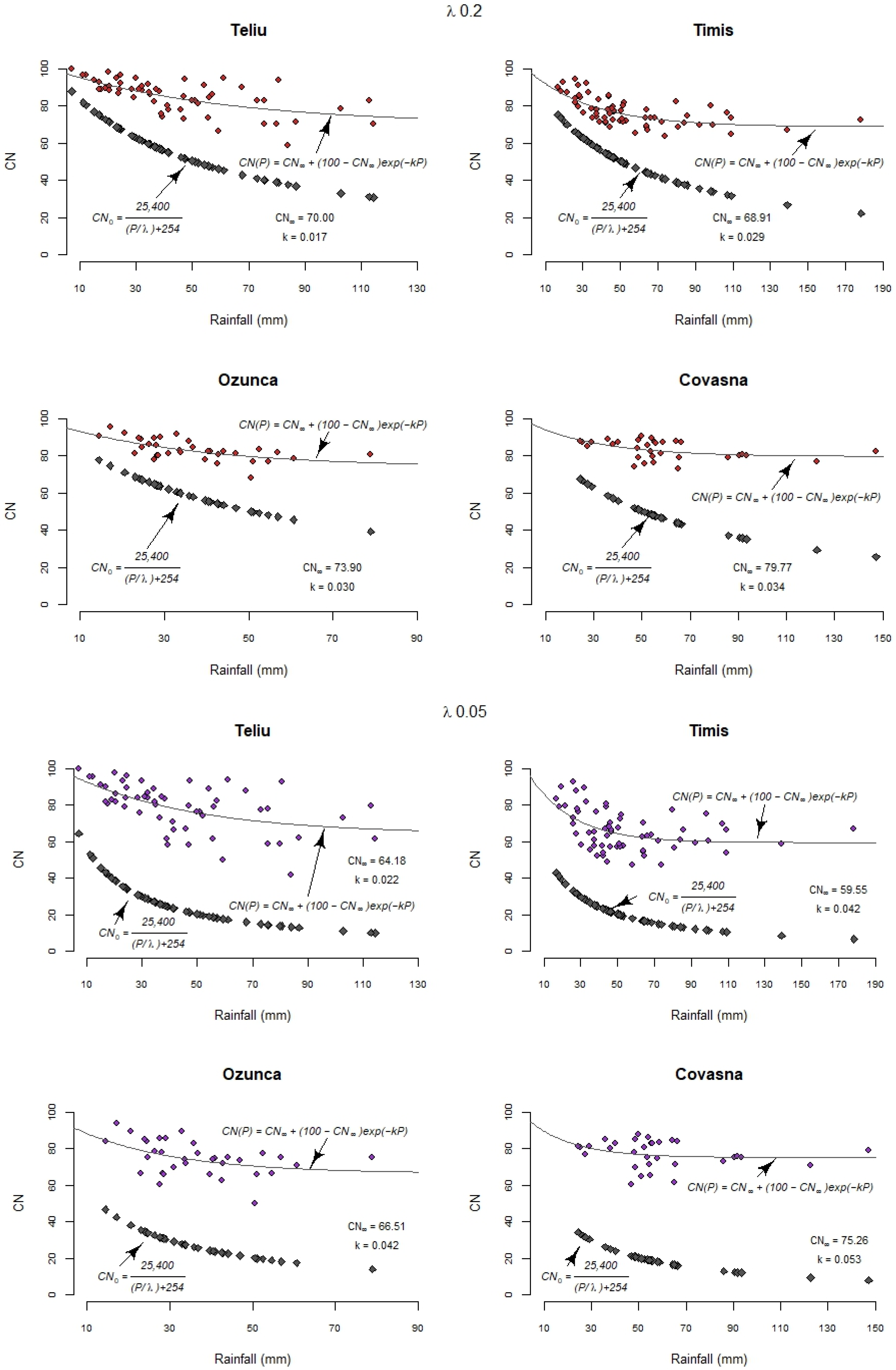
3.3.5. Asymptotic Fitting Method (AF)
3.4. Statistical Analysis for Performance Evaluation
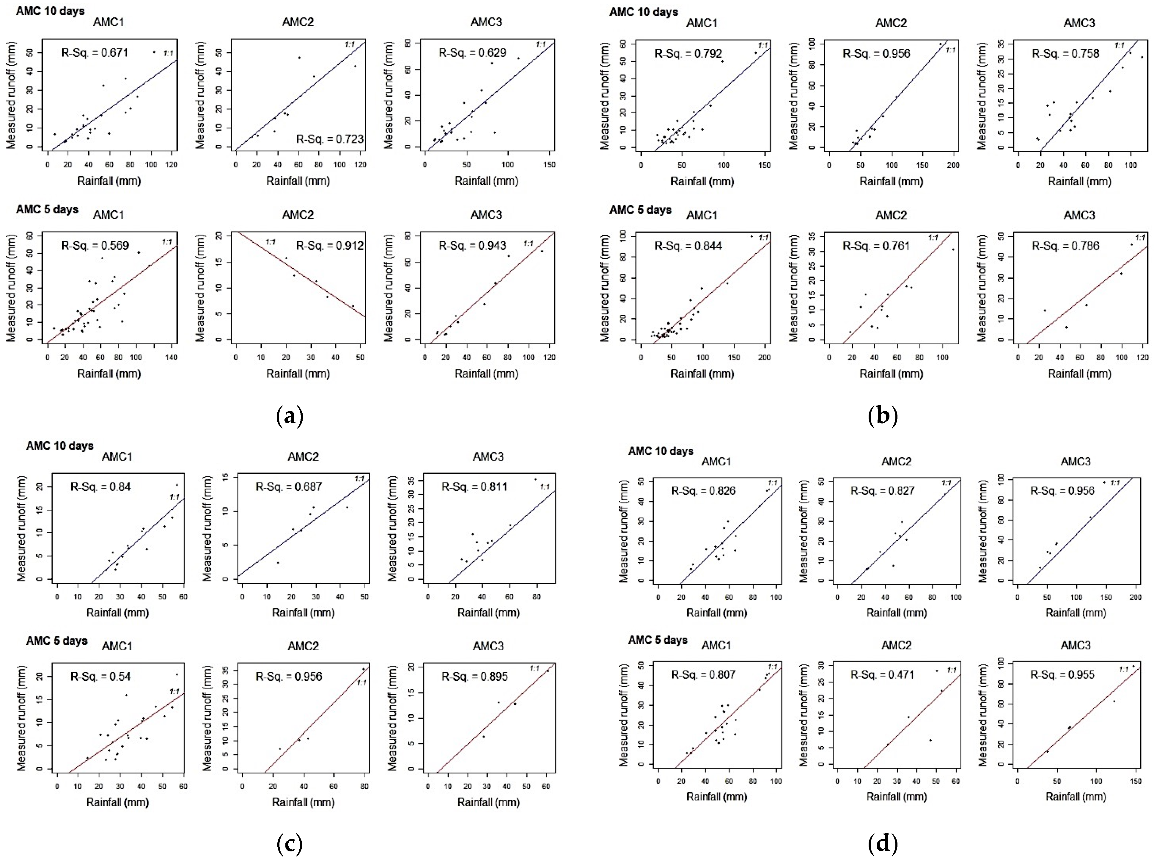
4. Results
5. Discussion
Limitations
6. Conclusions
Author Contributions
Funding
Data Availability Statement
Acknowledgments
Conflicts of Interest
References
- Hänsel, S.; Hoy, A.; Brendel, C.; Maugeri, M. Record summers in Europe: Variations in drought and heavy precipitation during 1901–2018. Int. J. Climatol. 2022, 42, 6235–6257. [Google Scholar] [CrossRef]
- Marchi, L.; Borga, M.; Preciso, E.; Gaume, E. Characterisation of selected extreme flash floods in Europe and implications for flood risk management. J. Hydrol. 2010, 394, 118–133. [Google Scholar] [CrossRef]
- Mrozik, K. Assessment of Retention Potential Changes as an Element of Suburbanization Monitoring on Example of an Ungauged Catchment in Poznan Metropolitan Area (Poland). Rocz. Ochr. Sr. 2016, 18, 188–200. [Google Scholar]
- Krvavica, N.; Rubinić, J. Evaluation of design storms and critical rainfall durations for flood prediction in partially urbanized catchments. Water 2020, 12, 2044. [Google Scholar] [CrossRef]
- Scopesi, C.; Maerker, M.; Bachofer, F.; Rellini, I.; Firpo, M. Assessment of flash floods in a small Mediterranean catchment using terrain analysis and remotely sensed data: A case study in the Torrente Teiro, Liguria, Italy. Z. Geomorphol. 2017, 61, 137–163. [Google Scholar] [CrossRef]
- Chatzichristaki, C.; Stefanidis, S.; Stefanidis, P.; Stathis, D. Analysis of the flash flood in Rhodes Island (South Greece) on 22 November 2013. Silva Balc. 2015, 16, 76–86. [Google Scholar]
- Sapountzis, M.; Stathis, D. Relationship between rainfall and run-off in the Stratoni Region (N. Greece) after the storm of 10th February 2010. Glob. Nest J. 2014, 16, 420–431. [Google Scholar]
- Petrović, A.M.; Novković, I.; Kostadinov, S. Hydrological analysis of the September 2014 torrential floods of the Danube tributaries in the Eastern Serbia. Nat. Hazards 2021, 108, 1373–1387. [Google Scholar] [CrossRef]
- Bucała-Hrabia, A.; Kijowska-Strugała, M.; Bryndal, T.; Cebulski, J.; Kiszka, K.; Kroczak, R. An integrated approach for investigating geomorphic changes due to flash flooding in two small stream channels (Western Polish Carpathians). J. Hydrol. Reg. Stud. 2020, 31, 100731. [Google Scholar] [CrossRef]
- Vojtek, M.; Vojtekova, J. Land use change and its impact on surface runoff from small basins: A case of Radiša Basin. Folia Geogr. 2019, 61, 104–125. [Google Scholar]
- Crăciun, A.I. Estimarea indirectă, cu ajutorul GIS, a umezelii solului în scopul modelării viiturilor pluviale. Aplicații în Munții Apuseni. Ph.D. Thesis, Babeș-Bolyai University, Cluj-Napoca, Romania, 2011; p. 278. [Google Scholar]
- Singh, C.B.; Kumre, S.K.; Mishra, S.K.; Singh, P.K. Effect of land use on curve number in steep watersheds. In Water Management and Water Governance: Hydrological Modeling; Pandey, A., Mishra, S.K., Kansal, M.L., Singh, R.D., Singh, V.P., Eds.; Springer: Cham, Switzerland, 2021; Volume 96, pp. 361–374. [Google Scholar]
- Ahmadi-Sani, N.; Razaghnia, L.; Pukkala, T. Effect of Land-Use Change on Runoff in Hyrcania. Land 2022, 11, 220. [Google Scholar] [CrossRef]
- Zhang, X.; Cao, W.; Guo, Q.; Wu, S. Effects of landuse change on surface runoff and sediment yield at different watershed scales on the Loess Plateau. Int. J. Sediment Res. 2010, 25, 283–293. [Google Scholar] [CrossRef]
- Admas, M.; Melesse, A.M.; Abate, B.; Tegegne, G. Soil Erosion, Sediment Yield, and Runoff Modeling of the Megech Watershed Using the GeoWEPP Model. Hydrology 2022, 9, 208. [Google Scholar] [CrossRef]
- Parhizkar, M.; Shabanpour, M.; Lucas-Borja, M.E.; Zema, D.A.; Li, S.; Tanaka, N.; Cerdà, A. Effects of Length and Application Rate of Rice Straw Mulch on Surface Runoff and Soil Loss under Laboratory Simulated Rainfall. Int. J. Sediment Res. 2021, 36, 468–478. [Google Scholar] [CrossRef]
- Ponce, V.M.; Hawkins, R.H. Runoff curve number: Has it reached maturity? J. Hydrol. Eng. 1996, 1, 11–19. [Google Scholar] [CrossRef]
- Mishra, S.K.; Singh, V.P. Soil Conservation Service Curve Number (SCS-CN) Methodology; Springer: Dordrecht, The Netherlands, 2003; Volume 42, p. 516. [Google Scholar]
- Ajmal, M.; Kim, T.-W.; Ahn, J.H. Stability assessment of the curve number methodology used to estimate excess rainfall in forest-dominated watersheds. Arab. J. Geosci. 2016, 9, 402. [Google Scholar] [CrossRef]
- Crăciun, A.I.; Haidu, I.; Magyari-Saska, Z.; Imbroane, A.I. Estimation of runoff coefficient according to soil moisture using GIS techniques. Geogr. Techol. 2009, 4, 1–10. [Google Scholar]
- Domnița, M.; Crăciun, A.I.; Haidu, I. GIS in determination of the discharge hydrograph generated by surface runoff for small basins. Geogr. Tech. 2009, 4, 10–22. [Google Scholar]
- Domniţa, M.; Crăciun, A.I.; Haidu, I.; Magyari-Saska, Z. Geographical Information System module for deriving the flash flood hydrograph in mountainous areas. In Proceedings of the 4th European Computing Conference, Bucharest, Romania, 20–22 April 2010. [Google Scholar]
- Domniţa, M.; Crăciun, A.I.; Haidu, I.; Magyari-Saska, Z. GIS used for determination of the maximum discharge in very small basins (under 2 km2). WSEAS Trans. Environ. Dev. 2010, 6, 468–477. [Google Scholar]
- Strapazan, C.; Petruț, M. Application of Arc Hydro and HEC-HMS model techniques for runoff simulation in the headwater areas of Covasna Watershed (Romania). Geogr. Tech. 2017, 12, 95–107. [Google Scholar] [CrossRef] [Green Version]
- Strapazan, C.; Haidu, I.; Kocsis, I. Assessing Land Use/Land Cover Change and its Impact on Surface Runoff in the Southern Part of the Țibleș and Rodnei Mountains. In Proceedings of the Air and Water—Components of the Environment, Cluj-Napoca, Romania, 22–24 March 2019; pp. 225–236. [Google Scholar]
- Strapazan, C.; Haidu, I.; Irimus, A.I. A comparative assessment of different loss methods available in Mike Hydro River-UHM. Carpathian J. Earth Environ. Sci. 2021, 16, 261–273. [Google Scholar] [CrossRef]
- Haidu, I.; Strapazan, C. Flash flood prediction in small to medium-sized watersheds. Case study: Bistra river (Apuseni Mountains, Romania). Carpathian J. Earth Environ. Sci. 2019, 14, 439–448. [Google Scholar]
- Hawkins, R.H.; Ward, T.J.; Woodward, D.E.; Van Mullem, J.A. Curve Number Hydrology-State of Practice; American Society of Civil Engineers: Reston, VI, USA, 2009; p. 106. [Google Scholar]
- Hawkins, R.H. Asymptotic determination of runoff curve numbers from data. J. Irrig. Drain. Eng. 1993, 119, 334–345. [Google Scholar] [CrossRef]
- Im, S.; Lee, J.; Kuraji, K.; Lai, Y.J.; Tuankrua, V.; Tanaka, N.; Gomyo, M.; Inoue, H.; Tseng, C.W. Soil Conservation Service curve number determination for forest cover using rainfall and runoff data in experimental forests. J. For. Res. 2020, 25, 204–213. [Google Scholar] [CrossRef]
- NRCS (Natural Resources Conservation Service). Chapter 9: Hydrologic Soil-Cover complexes. In Part 630: Hydrology, National Engineering Handbook; U.S. Department of Agriculture: Washington, DC, USA, 2004. Available online: https://directives.sc.egov.usda.gov/OpenNonWebContent.aspx?content=17758.wba (accessed on 15 February 2022).
- Ajmal, M.; Waseem, M.; Kim, D.; Kim, T.-W. A Pragmatic Slope-Adjusted Curve Number Model to Reduce Uncertainty in Predicting Flood Runoff from Steep Watersheds. Water 2020, 12, 1469. [Google Scholar] [CrossRef]
- Woodward, D.E.; Hawkins, R.H.; Jiang, R.; Hjelmfelt Junior, A.T.; Van Mullem, J.A.; Quan, D.Q. Runoff curve number method: Examination of the initial abstraction ratio. In Proceedings of the World Water & Environmental Resources Congress 2003, Philadelphia, PA, USA, 23–26 June 2003; pp. 1–10. [Google Scholar]
- Beck, H.E.; de Jeu, R.A.M.; Schellekens, J.; van Dijk, A.I.J.M.; Bruijnzeel, L.A. Improving Curve Number Based Storm Runoff Estimates Using Soil Moisture Proxies. IEEE J. Sel. Top. Appl. Earth Obs. Remote Sens. 2009, 2, 250–259. [Google Scholar] [CrossRef]
- D’Asaro, F.; Grillone, G.; Hawkins, R.H. Curve number: Empirical evaluation and comparison with curve number handbook tables in Sicily. J. Hydrol. Eng. 2014, 19, 04014035. [Google Scholar] [CrossRef]
- Wałega, A.; Młynski, D.; Wachulec, K. The use of asymptotic functions for determining empirical values of CN parameter in selected catchments of variable land cover. Stud. Geotech. Mech 2017, 39, 111–120. [Google Scholar] [CrossRef] [Green Version]
- Valle Junior, L.C.G.; Rodrigues, D.B.B.; de Oliveira, P.T.S. Initial abstraction ratio and curve number estimation using rainfall and runoff data from a tropical watershed. Rev. Bras. Recur. Hídr. 2019, 24, 1–9. [Google Scholar] [CrossRef] [Green Version]
- Cao, H.; Vervoort, R.W.; Dabney, S.M. Variation of curve number derived from plot runoff data for New South Wales (Australia). Hydrol. Process. 2011, 25, 3774–3789. [Google Scholar] [CrossRef]
- Tedela, N.H.; McCutcheon, S.C.; Rasmussen, T.C.; Hawkins, R.H.; Swank, W.T.; Campbell, J.L.; Adams, M.B.; Jackson, C.R.; Tollner, E.W. Runoff curve numbers for 10 small forested watersheds in the mountains of the eastern United States. J. Hydrol. Eng. 2012, 17, 1188–1198. [Google Scholar] [CrossRef] [Green Version]
- Farran, M.M.; Elfeki, A.M. Variability of the asymptotic curve number in mountainous undeveloped arid basins based on historical data: Case study in Saudi Arabia. J. Afr. Earth Sci. 2020, 162, 103697. [Google Scholar] [CrossRef]
- Calero-Mosquera, D.; Hoyos-Villada, F.; Torres-Prieto, E. Runoff Curve Number (CN model) Evaluation Under Tropical Conditions. Earth Sci. Res. J. 2021, 25, 397–404. [Google Scholar] [CrossRef]
- Mishra, S.K.; Jain, M.K.; Babu, P.S.; Venugopal, K.; Kaliappan, S. Comparison of AMC-dependent CN-conversion formulae. Water Resour. Manag 2008, 22, 1409–1420. [Google Scholar] [CrossRef]
- Ibrahim, S.; Brasi, B.; Yu, Q.; Siddig, M.S. Curve number estimation using rainfall and runoff data from five catchments in Sudan. Open Geosci. 2022, 14, 294–303. [Google Scholar] [CrossRef]
- Hjelmfelt, A.T. Investigation of curve number procedure. J. Hydraul. Eng. 1991, 117, 725–737. [Google Scholar] [CrossRef]
- Walega, A.; Michalec, B.; Cupak, A.; Grzebinoga, M. Comparison of SCS-CN Determination Methodologies in a heterogeneous catchment. J. Mt. Sci. 2015, 12, 1084–1094. [Google Scholar] [CrossRef]
- Hawkins, R.; Hjelmfelt, J.A.; Zevenbergen, A. Runoff probability, storm depth and curve numbers. J. Irrig. Drain. Div. 1985, 111, 330–340. [Google Scholar] [CrossRef]
- Corbuș, C. Programul CAVIS pentru determinarea caracteristicilor undelor de viitură singulare. In Proceedings of the INHGA Jubilee Scientific Conference, ”Hydrology and Water Management—2025 Challenges for the Sustainable Development of Water Resources, Bucharest, Romania, 28–30 September 2010. (In Romanian). [Google Scholar]
- Chendeș, V. Resursele de apa din Subcarpatii de la Curbura. Evaluari Geospatiale; Editura Academiei Romane: Bucharest, Romania, 2011; p. 340. [Google Scholar]
- Cole, B.; Smith, G.; de la Barreda-Bautista, B.; Hamer, A.; Payne, M.; Codd, T.; Johnson, S.C.M.; Chan, L.Y.; Balzter, H. Dynamic Landscapes in the UK Driven by Pressures from Energy Production and Forestry—Results of the CORINE Land Cover Map 2018. Land 2022, 11, 192. [Google Scholar] [CrossRef]
- SCS (Soil Conservation Service). National Engineering Handbook, Section 4: Hydrology; U.S. Soil Conservation Service: Washington, DC, USA, 1964. [Google Scholar]
- Hawkins, R.H.; Theurer, F.D.; Rezaeianzadeh, M. Understanding the basis of the curve number method for watershed models and TMDLs. J. Hydrol. Eng. 2019, 24, 06019003. [Google Scholar] [CrossRef]
- Hawkins, R.H.; Ward, T.J.; Woodward, D.E.; Van Mullem, J.A. Continuing evolution of rainfall-runoff and the curve number precedent. In Proceedings of the 2nd Joint Federal Interagency Conference, Las Vegas, NV, USA, 27 June–1 July 2010; pp. 1–12. [Google Scholar]
- Gundalia, M.; Dholakia, M. Impact of antecedent runoff condition on curve number determination and performance of SCS-CN model Forozat catchment in India. Int. J. Civ. Struct. Environ. Infrastruct. Eng. Res. Dev. 2014, 4, 87–100. [Google Scholar]
- Elzhov, T.V.; Mullen, K.M.; Spiess, A.-N.; Bolker, B. Minpack.lm: R Interface to the Levenberg-Marquardt Nonlinear least-Squares Algorithm Found in MINPACK, Plus Support for Bounds. 2022. Available online: https://CRAN.R-project.org/package=minpack.lm (accessed on 3 August 2022).
- R Core Team. R: A language and environment for statistical computing. R Foundation for Statistical Computing. Vienna, Austria. Available online: https://www.R-project.org/ (accessed on 13 September 2022).
- R Studio Team. R Studio: Integrated Development for R. Rstudio. PBC, Boston, MA. Available online: http://www.rstudio.com/ (accessed on 13 September 2022).
- Moriasi, D.N.; Arnold, J.G.; Van Liew, M.W.; Bingner, R.L.; Harmel, R.D.; Veith, T.L. Model evaluation guidelines for systematic quantification of accuracy in watershed simulations. Trans. ASABE 2007, 50, 885–900. [Google Scholar] [CrossRef]
- Diaz-Ramirez, J.N.; McAnally, W.H.; Martin, J.L. Analysis of hydrological processes applying the HSPF model in selected watersheds in Alabama, Mississippi, and Puerto Rico. Appl. Eng. Agric. 2011, 27, 937–954. [Google Scholar] [CrossRef]
- Ritter, A.; Muñoz-Carpena, R. Performance evaluation of hydrological models: Statistical significance for reducing subjectivity in goodness-of-fit assessments. J. Hydrol. 2013, 480, 33–45. [Google Scholar] [CrossRef]
- Ajmal, M.; Moon, G.; Ahn, J.; Kim, T.-W. Investigation of SCS-CN and its inspired modified models for runoff estimation in South Korean watersheds. J. Hydro-Environ. Res. 2015, 9, 592–603. [Google Scholar] [CrossRef]
- Willmott, C.J. On the validation of models. Phys. Geogr. 1981, 2, 184–194. [Google Scholar] [CrossRef]
- Zambrano-Bigiarini, M. Package hydroGOF: Goodness-of-Fit Functions for Comparison of Simulated and Observed Hydrological Time Series. 2020. Available online: https://cran.r-project.org/web/packages/hydroGOF/hydroGOF.pdf (accessed on 6 September 2022).
- Randusova, B.; Markova, R.; Kohnova, S.; Hlavcova, K. Comparison of CN estimation approaches. Int. J. Eng. Res.Sc. 2015, 1, 34–40. [Google Scholar]
- Kowalik, T.; Walega, A. Estimation of CN parameter for small agricultura watersheds using asymptotic functions. Water 2015, 7, 939–955. [Google Scholar] [CrossRef] [Green Version]
- Rutkowska, A.; Kohnová, S.; Banasik, K.; Szolgay, J.; Karabova, B. Probabilistic properties of a curve number: A case study for small Polish and Slovak Carpathian Basins. J. Mt. Sci. 2015, 12, 533–548. [Google Scholar] [CrossRef]
- Niyazi, B.; Khan, A.A.; Masoud, M.; Elfeki, A.; Basahi, J.; Zaidi, S. Optimum parametrization of the soil conservation service (SCS) method for simulating the hydrological response in arid basins. Geomat. Nat. Hazards Risk 2022, 13, 1482–1509. [Google Scholar] [CrossRef]
- Baltas, E.A.; Dervos, N.A.; Mimikou, M.A. Technical Note: Determination of the SCS initial abstraction ratio in an experimental watershed in Greece. Hydrol. Earth Sys. Sci. 2007, 11, 1825–1829. [Google Scholar] [CrossRef] [Green Version]
- Mishra, S.K.; Babu, P.S.; Singh, V.P. SCS-CN Method Revisited. In Advances in Hydraulics and Hydrology; Water Resources Publications: Littleton, CO, USA, 2007. [Google Scholar]


| Watershed | Area (km2) | Mean Elevation (m) | Average Slope (%) | Hydrometric Station | The Time Range of the Observational Data Used in the Study | No. of Events |
|---|---|---|---|---|---|---|
| Teliu | 36 | 801 | 24.92 | Teliu | 1991–2020 | 57 |
| Timis | 75 | 1108 | 36.43 | Db. Morii | 1993–2020 | 64 |
| Ozunca | 66 | 746 | 16.66 | Batanii Mari | 2004–2018 | 34 |
| Covasna | 39 | 1037 | 29.39 | Covasna | 2004–2018 | 32 |
| Watershed | Forests | Urban Areas | Pastures | Heterogeneous Agricultural Areas | Scrub and/or Herbaceous Vegetation Associations | Arable Lands | Artificial, Non-Agricultural Vegetated Areas | |||||||
|---|---|---|---|---|---|---|---|---|---|---|---|---|---|---|
| km2 | % | km2 | % | km2 | % | km2 | % | km2 | % | km2 | % | km2 | % | |
| Teliu | 25.41 | 70.5 | 1.11 | 3.1 | 7.44 | 20.7 | 1.49 | 4.1 | 0.57 | 1.6 | ||||
| Timiș | 69.31 | 92.4 | 1.90 | 2.5 | 0.60 | 0.8 | 1.39 | 1.9 | 1.21 | 1.6 | 0.60 | 0.8 | ||
| Ozunca | 36.75 | 55.5 | 0.33 | 0.5 | 5.67 | 8.6 | 2.74 | 4.1 | 15.53 | 23.5 | 5.19 | 7.8 | ||
| Covasna | 31.77 | 81.5 | 0.59 | 1.5 | 0.18 | 0.5 | 6.43 | 16.5 | ||||||
| Watershed | MD | GM | AM | AFO | AFN | Behavior | TAB | ||
|---|---|---|---|---|---|---|---|---|---|
| CNAFo (R2, SE) | k (SE) | CNAFn (R2, SE) | k (SE) | ||||||
| Teliu | 85.85 | 85.89 | 85.06 | 80.45 (0.94, 0.438) | 0.034 (0.002) | 70.00 (0.43, 7.228) | 0.017 (0.007) | Standard | 54.00 |
| Timiș | 76.52 | 79.55 | 77.99 | 71.98 (0.88, 0.442) | 0.038 (0.002) | 68.91 (0.51, 2.081) | 0.029 (0.005) | Standard | 50.00 |
| Ozunca | 83.12 | 84.29 | 83.69 | 79.58 (0.80, 0.664) | 0.049 (0.004) | 73.90 (0.43, 4.970) | 0.030 (0.011) | Standard | 73.00 |
| Covasna | 82.56 | 83.98 | 83.45 | 81.87 (0.23 0.883) | 0.050 (0.011) | 79.77 (0.19 2.311) | 0.034 (0.011) | Standard | 61.00 |
| Watershed | MD | GM | AM | AFO | AFN | Behavior | TAB | ||
|---|---|---|---|---|---|---|---|---|---|
| CNAFo (R2, SE) | k (SE) | CNAFn (R2, SE) | k (SE) | ||||||
| Teliu | 80.88 | 80.89 | 79.81 | 75.61 (0.89, 0.524) | 0.046 (0.003) | 64.18 (0.33 7.504) | 0.022 (0.009) | Standard | 39.03 |
| Timiș | 66.96 | 71.43 | 69.67 | 63.91 (0.64, 0.476) | 0.066 (0.005) | 59.55 (0.30, 2.697) | 0.042 (0.009) | Standard | 34.74 |
| Ozunca | 75.27 | 77.19 | 76.36 | 73.84 (0.29, 0.687) | 0.092 (0.013) | 66.51 (0.24, 5.890) | 0.042 (0.017) | Standard | 62.56 |
| Covasna | 79.04 | 78.97 | 78.23 | 77.09 (0.03, 0.810) | 0.103 (0.051) | 75.26 (0.054, 2.470) | 0.053 (0.025) | Standard | 47.10 |
| Watershed | The Rainfall-Driven Runoff Event that Occurred from 27th of June to 4th of July 2018 | The Entire Rainfall–Runoff Series | ||||
|---|---|---|---|---|---|---|
| Runoff Coefficient (C) | q L/s/kmp | CN 0.2 | CN 0.05 | Highest Runoff Coefficient (C) Value | q L/s/kmp | |
| Timiș | 0.42 | 264 | 73.9 | 66.7 | 0.56 | 747 |
| Covasna | 0.51 | 359 | 76.8 | 71.1 | 0.67 | 669 |
| Teliu | 0.61 | 1750 | 83.3 | 79.5 | 0.8 | 1750 |
| Ozunca | 0.32 | 721 | 78.9 | 70.9 | 0.49 | 962 |
| λ = 0.2 | ||||||
|---|---|---|---|---|---|---|
| Watershed | Method | R2 | NSE | RMSE | PBIAS (%) | d |
| Teliu | MD | 0.751 | 0.678 | 9.850 | 6.6 | 0.924 |
| GM | 0.751 | 0.677 | 9.870 | 6.8 | 0.924 | |
| AM | 0.751 | 0.698 | 9.550 | 2.2 | 0.927 | |
| AFO | 0.749 | 0.650 | 10.26 | −20.1 | 0.907 | |
| AFN | 0.734 | −0.044 | 17.755 | −57.8 | 0.721 | |
| TAB | 0.387 | −0.669 | 22.45 | −69.2 | 0.596 | |
| Timis | MD | 0.925 | 0.872 | 8.096 | 4.2 | 0.973 |
| GM | 0.921 | 0.770 | 10.829 | 19.0 | 0.955 | |
| AM | 0.923 | 0.833 | 9.240 | 11.2 | 0.966 | |
| AFO | 0.929 | 0.890 | 7.487 | −15.5 | 0.974 | |
| AFN | 0.929 | 0.831 | 9.294 | −27.4 | 0.957 | |
| TAB | 0.313 | −0.122 | 23.948 | −57.5 | 0.635 | |
| Ozunca | MD | 0.769 | 0.592 | 4.487 | −0.6 | 0.920 |
| GM | 0.765 | 0.510 | 4.910 | 8.5 | 0.908 | |
| AM | 0.767 | 0.559 | 4.660 | 3.8 | 0.916 | |
| AFO | 0.780 | 0.529 | 4.820 | −24.4 | 0.897 | |
| AFN | 0.796 | −0.128 | 7.458 | −53.5 | 0.751 | |
| TAB | 0.663 | −0.169 | 7.591 | −19.5 | 0.829 | |
| Covasna | MD | 0.903 | 0.872 | 7.108 | −3.6 | 0.971 |
| GM | 0.903 | 0.861 | 7.390 | 2.9 | 0.969 | |
| AM | 0.903 | 0.868 | 7.196 | 0.4 | 0.971 | |
| AFO | 0.903 | 0.867 | 7.230 | −6.7 | 0.969 | |
| AFN | 0.906 | 0.819 | 8.439 | −15.6 | 0.957 | |
| TAB | 0.784 | −0.329 | 22.877 | −57.2 | 0.779 | |
| λ = 0.05 | ||||||
|---|---|---|---|---|---|---|
| Watershed | Method | R2 | NSE | RMSE | PBIAS (%) | d |
| Teliu | MD | 0.752 | 0.717 | 9.237 | 4.5 | 0.928 |
| GM | 0.752 | 0.717 | 9.239 | 4.5 | 0.928 | |
| AM | 0.752 | 0.729 | 9.038 | 0.5 | 0.930 | |
| AFO | 0.745 | 0.394 | 13.529 | −39.7 | 0.830 | |
| AFN | 0.745 | 0.298 | 14.558 | −43.3 | 0.785 | |
| TAB | 0.590 | −0.715 | 22.755 | −75.9 | 0.612 | |
| Timis | MD | 0.925 | 0.916 | 6.537 | −1.7 | 0.980 |
| GM | 0.921 | 0.893 | 8.414 | 12.9 | 0.970 | |
| AM | 0.923 | 0.911 | 7.396 | 7.0 | 0.976 | |
| AFO | 0.925 | 0.911 | 6.759 | −10.8 | 0.977 | |
| AFN | 0.927 | 0.853 | 8.665 | −22.9 | 0.959 | |
| TAB | 0.473 | −0.107 | 23.785 | −65.0 | 0.651 | |
| Ozunca | MD | 0.771 | 0.709 | 3.790 | −3.1 | 0.933 |
| GM | 0.767 | 0.662 | 4.083 | 5.5 | 0.927 | |
| AM | 0.769 | 0.690 | 3.913 | 1.7 | 0.931 | |
| AFO | 0.773 | 0.708 | 3.792 | −9.1 | 0.930 | |
| AFN | 0.783 | 0.391 | 5.478 | −34.8 | 0.840 | |
| TAB | 0.678 | 0.085 | 6.716 | −14.3 | 0.853 | |
| Covasna | MD | 0.905 | 0.886 | 6.699 | 1.9 | 0.973 |
| GM | 0.906 | 0.887 | 6.679 | 1.7 | 0.973 | |
| AM | 0.906 | 0.891 | 6.544 | −0.7 | 0.974 | |
| AFO | 0.906 | 0.891 | 6.556 | −4.3 | 0.974 | |
| AFN | 0.906 | 0.873 | 7.064 | −9. | 0.968 | |
| TAB | 0.791 | −0.236 | 22.068 | −56.6 | 0.775 | |
Disclaimer/Publisher’s Note: The statements, opinions and data contained in all publications are solely those of the individual author(s) and contributor(s) and not of MDPI and/or the editor(s). MDPI and/or the editor(s) disclaim responsibility for any injury to people or property resulting from any ideas, methods, instructions or products referred to in the content. |
© 2023 by the authors. Licensee MDPI, Basel, Switzerland. This article is an open access article distributed under the terms and conditions of the Creative Commons Attribution (CC BY) license (https://creativecommons.org/licenses/by/4.0/).
Share and Cite
Strapazan, C.; Irimuș, I.-A.; Șerban, G.; Man, T.C.; Sassebes, L. Determination of Runoff Curve Numbers for the Growing Season Based on the Rainfall–Runoff Relationship from Small Watersheds in the Middle Mountainous Area of Romania. Water 2023, 15, 1452. https://doi.org/10.3390/w15081452
Strapazan C, Irimuș I-A, Șerban G, Man TC, Sassebes L. Determination of Runoff Curve Numbers for the Growing Season Based on the Rainfall–Runoff Relationship from Small Watersheds in the Middle Mountainous Area of Romania. Water. 2023; 15(8):1452. https://doi.org/10.3390/w15081452
Chicago/Turabian StyleStrapazan, Carina, Ioan-Aurel Irimuș, Gheorghe Șerban, Titus Cristian Man, and Laura Sassebes. 2023. "Determination of Runoff Curve Numbers for the Growing Season Based on the Rainfall–Runoff Relationship from Small Watersheds in the Middle Mountainous Area of Romania" Water 15, no. 8: 1452. https://doi.org/10.3390/w15081452