

High Resolution Estimation of Ocean Dissolved Inorganic Carbon, Total Alkalinity and pH Based on Deep Learning

1
Institute of Earth Systems, University of Malta, MSD 2080 Msida, Malta
2
Department of Physics and Astronomy (DIFA), Alma Mater Studiorum—Università di Bologna, 40126 Bologna, Italy
3
Interdepartmental Research Centre for Environmental Sciences (CIRSA), University of Bologna, 48123 Ravenna, Italy
*
Author to whom correspondence should be addressed.
Water 2023, 15(8), 1454; https://doi.org/10.3390/w15081454
Submission received: 25 February 2023
/
Accepted: 3 April 2023
/
Published: 7 April 2023
(This article belongs to the Topic Water Management in the Era of Climatic Change)
Abstract
:This study combines measurements of dissolved inorganic carbon (DIC), total alkalinity (TA), pH, earth observation (EO), and ocean model products with deep learning to provide a good step forward in detecting changes in the ocean carbonate system parameters at a high spatial and temporal resolution in the North Atlantic region (Long. −61.00° to −50.04° W; Lat. 24.99° to 34.96° N). The in situ reference dataset that was used for this study provided discrete underway measurements of DIC, TA, and pH collected by M/V Equinox in the North Atlantic Ocean. A unique list of co-temporal and co-located global daily environmental drivers derived from independent sources (using satellite remote sensing, model reanalyses, empirical algorithms, and depth soundings) were collected for this study at the highest possible spatial resolution (0.04° × 0.04°). The resulting ANN-estimated DIC, TA, and pH obtained by deep learning shows a high correspondence when verified against observations. This study demonstrates how a select number of geophysical information derived from EO and model reanalysis data can be used to estimate and understand the spatiotemporal variability of the oceanic carbonate system at a high spatiotemporal resolution. Further methodological improvements are being suggested.
1. Introduction
The global oceans constitute an important component in the global carbon cycle. They are also a major sink of human-induced emissions of CO2. When CO2 dissolves under typical ocean surface conditions, 90% of this CO2 is formed as HCO3−, 9% as HCO32−, and only 1% as undissociated CO2 (aq) and H2CO3 [1]. The four important parameters that are needed to understand the ocean carbonic acid system include the dissolved inorganic carbon (DIC), the total alkalinity (TA), the pH, and the pCO2 in surface water.
In the past decades, most of our understanding of the ocean carbonate system is derived from in situ observations. Now, thanks to global networking programs, observations have increased widely and consistently, due to ship surveys, the ARGOS project, and mooring and autonomous platforms; furthermore, due to the availability of ever more complex biogeochemical models, the understanding of ocean global and regional carbonate system has advanced considerably. These activities provide accurate, long-term time series fCO2 datasets, such as those found in the Surface Ocean CO2 Atlas—SOCAT—[2,3] and the Global Ocean Data Analysis Project (GLODAPv2.2022), consisting of data products of biogeochemical data collected through the chemical analysis of water samples, including TA, DIC, and many others [4]. This information now shows that surface ocean waters show around a 26% increase in concentration of hydrogen ions since 1860, which is equivalent to a drop in pH from 8.2 to 8.1 [5]. This change has been mainly attributed to the rising anthropogenic emissions of CO2 [5].
From a measurement point of view, changes in pH occur on a large spatial scale and can be influenced by different environmental parameters, especially at the local scale. Due to their very nature, direct field measurements are inherently limited in spatial (time series, moored stations) and/or temporal resolution (ship surveys). Earth observation (EO), on the other hand, offers an avenue for expanding observations and analyzing the temporal and spatial variability of the global ocean and its properties. While EO has proved to be a difficult tool for the direct monitoring of seawater pH and its impact on marine organisms, satellite remote sensing can indirectly measure this by providing us with a range of related physico-chemical and biological processes occurring at the ocean surface at an unprecedented spatiotemporal scale. In addition, even though in situ surface measurements offer a geographically limited representation of the entire oceanic volume and its contents, remote sensing observations of the global ocean become very important for the study of the carbonate system, due to the fact that the change in ocean chemistry arises first in the ocean surface. Thus, environmental satellites have great potential in this field.
At the local level, coastal communities are most vulnerable to a lowering pH, especially where the ocean chemistry is changing most rapidly due to multiple stressors. These communities have the potential of being the worst hit, both economically and socially, especially those who derive benefits from calcifying organisms and other vulnerable species [6]. This explains the need for the rapid monitoring of such coastal waters.
This study asks the following research questions: (1) how can we provide information on the state of ocean carbonate information (such as pH and other important carbonate chemistry parameters) at suitable geographical scales that are useful for the management of marine resources? and (2) how can a more robust monitoring of the ocean carbonate system be made available; one that is chemically, biologically, and physically linked to a good number of environmental drivers instead of a much smaller number of parameters, such as salinity, temperature, and chlorophyll? [7].
In seeking to address these research questions, this study moves away from others that have modeled ocean carbonate parameters at coarse temporal [8] and spatial scales (around 500–1500 km; [9]). Instead, it aims to provide ocean carbonate system parameter information at an unmatched high spatial (4 km) and temporal (such as daily) level via gridded ocean maps, with the opportunity of assimilating this into daily operational monitoring and forward the modeling that is used by a wide variety of ocean end users. This goes perfectly in line with NOAA-SOCAN’s top research priorities, i.e., “to monitor key ocean parameters across various spatial and temporal scales that will provide information on mechanistic drivers of acidification and input parameters for predictive model algorithm development” (known as ‘priority 1′) by developing “operational and qualitative models that can transition to end users and adapting existing models to understand acidification” (known as ‘priority 3′) from a “regional perspective as well as in specific systems” [10]. The end-user sectors of this data may range from artisanal and small-scale or semi-industrial fisheries and bivalve aquaculture [11] to coastal managers and policy makers whose actions need to become more adaptive in the short term.
To resolve this challenging aim, this study uses the artificial neural network (ANN) method to fix those specific, inter-related environmental conditions that can lead to particular states of the ocean carbonate system. It does so by following the approach that has been taken by the latest ocean research that uses time-finite, individual-ship-based transect measurements that cross extended oceanic areas such as the North Atlantic Ocean [12], the northwest European shelf seas [13], and the North Pacific Ocean [14], among others.
The calculations that have been carried out in this study were performed at a very high spatiotemporal resolution of a so-far unique list of environmental drivers that, in combination, are able to describe and model the much-needed detailed spatiotemporal variation of surface DIC, TA, and pH. This approach can lead to the prediction of a unique set of high-resolution, daily DIC, TA, and pH regional ocean surface grid maps, with potential applications in future studies focused on the local dynamics of the carbonate systems in both coastal and oceanic areas.
Now, the vast availability of daily EO data and related ancillary data are ideally suited for the ANN’s model-free estimators and for predictive data mining. In this study, the ANN allows the processing of different chemical, biological, and physical ocean values by estimating the most probable field values on the basis of their previous patterns, as observed out in the field. Depending on the algorithmic architecture, the ANN is able to perform its estimations through association, clustering, and prediction of the required output variables. While keeping in mind the practicality and the feasibility of this study, it is very important to create an ANN architecture that is able to learn, and ultimately model, the association between the ocean carbonate parameters and the largest possible number of oceanic physicochemical and biological processes. The potential use of such a tool can be extremely important for the validation of numerical ocean modeling and the prediction of changes in ocean carbonate chemistry.
2. Materials and Methods
2.1. Study Area
The study area covers part of the Atlantic Ocean, comprising part of the Iberian Plain, with the Canary basin on the east side and the North American basin on the western side, reaching to the Puerto Rico trench.
Time series measurements show that the North and Central Atlantic constitutes the largest reservoir of anthropogenic CO2 [15,16,17] and displays a surface ocean pH decline [18]. Moreover, a strong correlation between the pCO2 and the surface water pH was identified by Bates et al., 2012 [19], with the latter showing a definitive decrease in the North Atlantic Ocean between 1984 and 2012. Furthermore, in its 2015 and 2016 State of the Climate, NOAA reported a world record in terms of large sea surface temperature and upper ocean heat content anomalies in large swaths of the western North Atlantic Ocean [20,21]. This extreme event can offer an interesting opportunity to continue studying the changes in DIC, with respect to pH, TA, and sea temperature [22], whilst making use of the novelty of this study.
2.2. Field Data
This study made use of the best surface underway data available over the study area for the period of 2015–2016. The Ocean Carbon and Acidification Data Portal of the National Centers for Environmental Information provides only one set of surface underway data (NCEI Accession 0154382) that contains the three core study variables of DIC, TA, and pH over the study area covering the period of analysis (https://www.ncei.noaa.gov/data/oceans/ncei/ocads/metadata/0154382.html (accessed on 20 February 2023)). Additional surface underway datasets are available; however, these consist of an increasingly limited number of observations (such as NCEI Accession 0157237, 0157352, 0157312, and 0110259), for which suitable co-located and co-temporal satellite and model reanalysis data are not available.
2.2.1. In Situ Observations of the Carbonate System
From 7 March 2015 to 6 November 2016, the M/V Equinox (ID: MLCE) sailed across the North Atlantic Ocean three times. Discrete surface underway measurements of seawater DIC, TA, and pH were performed on all cruises (Figure 1). The details of the laboratory methods onboard the M/V Equinox are well documented [23] as NCEI Accession 0154382. This research was conducted in support of the coastal monitoring and research objectives of the NOAA Ocean Acidification Program (OAP) and the Climate Program Office. The research cruise covered an area from −78.9797° W to −10.3998° E and from 38.4622° N to 19.2893° S.
In addition to DIC, TA, and pH, M/V Equinox also collected sea surface temperature and sea surface salinity measurements with a documented uncertainty of ±0.001 °C and ±0.005%, respectively (see https://www.ncei.noaa.gov/data/oceans/ncei/ocads/metadata/0154382.html (accessed on 20 February 2023)). The range of the values collected during the cruise mission is shown in Table 1.
2.2.2. Remote Sensing Data and Reanalysis Data
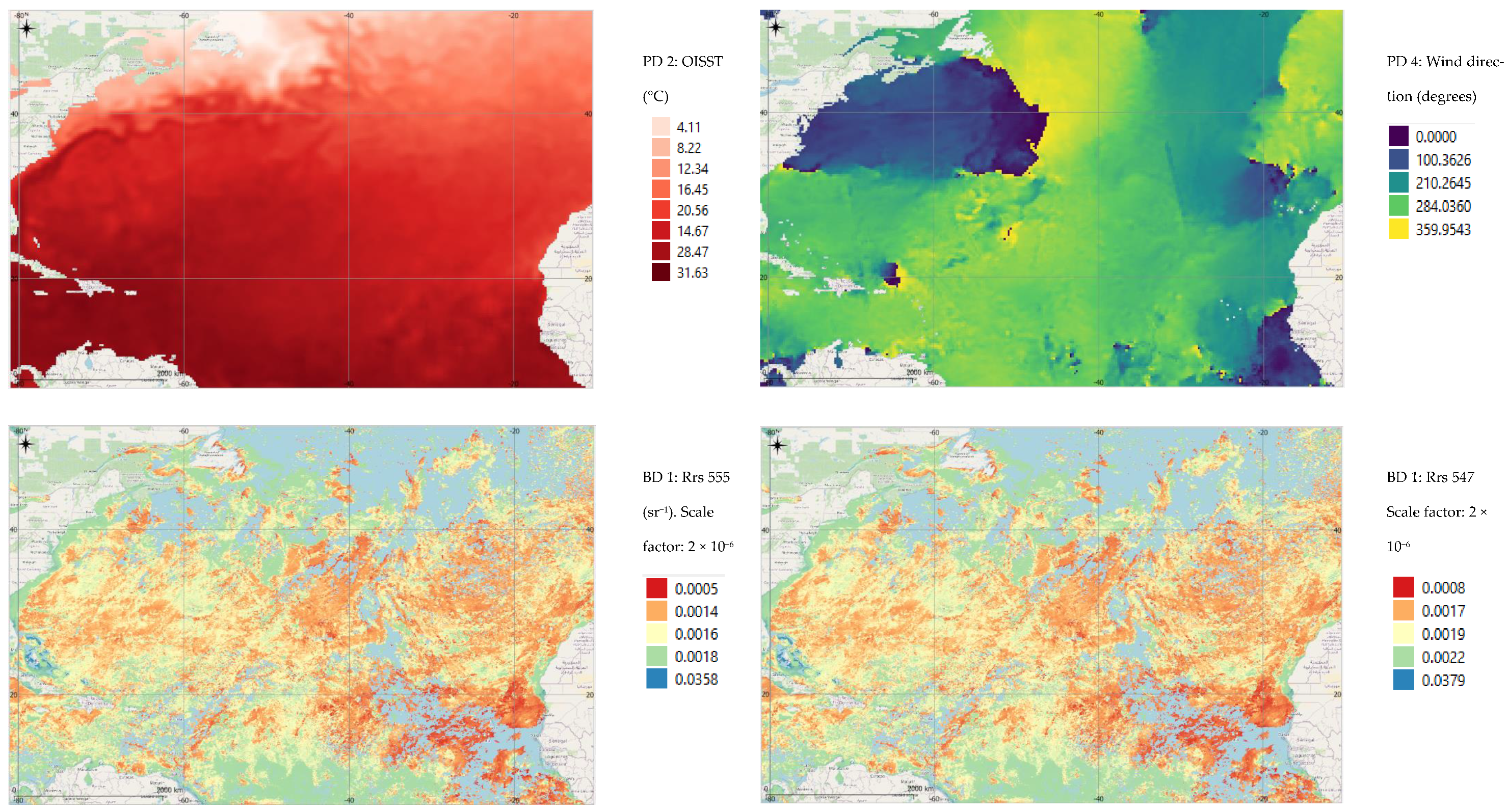
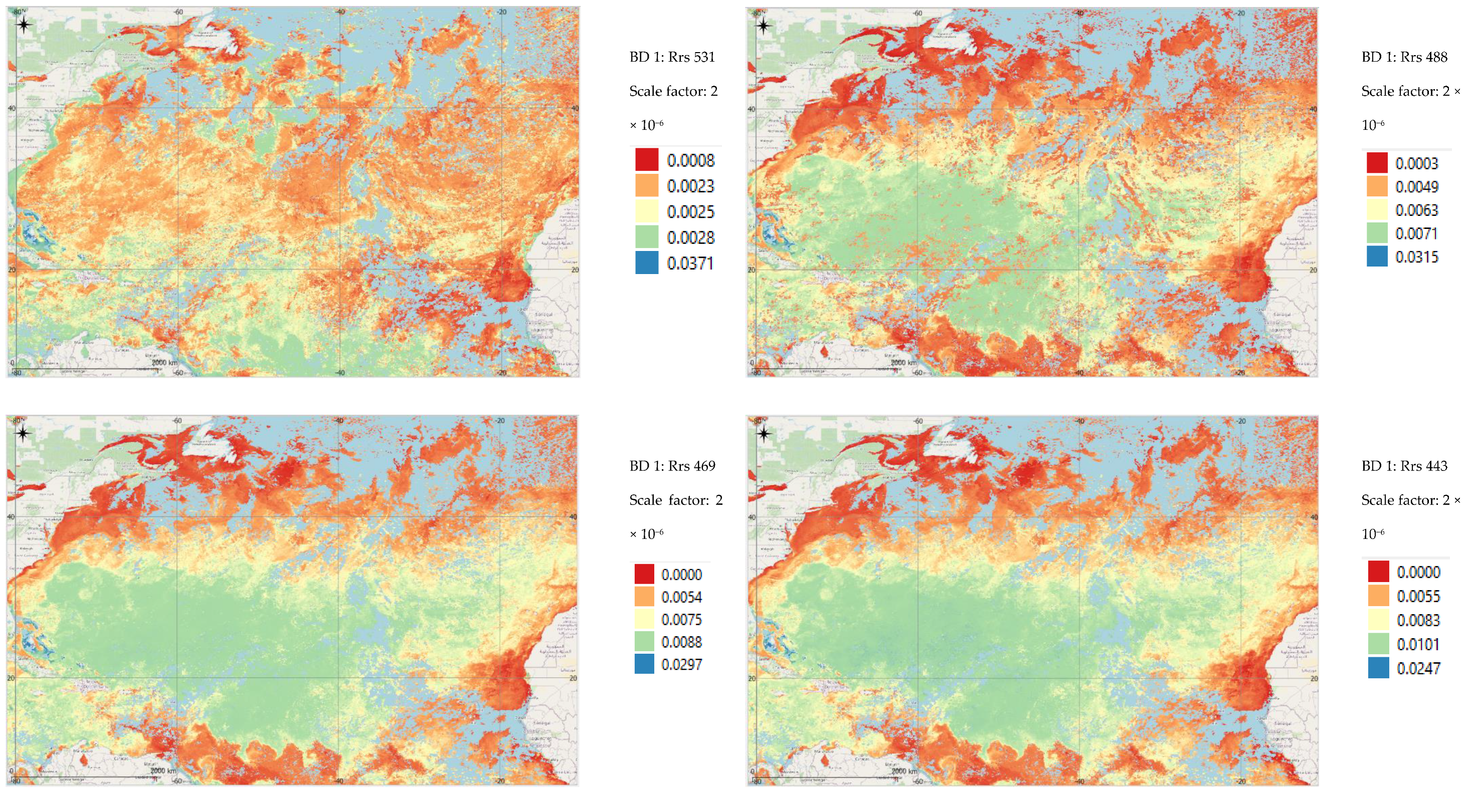
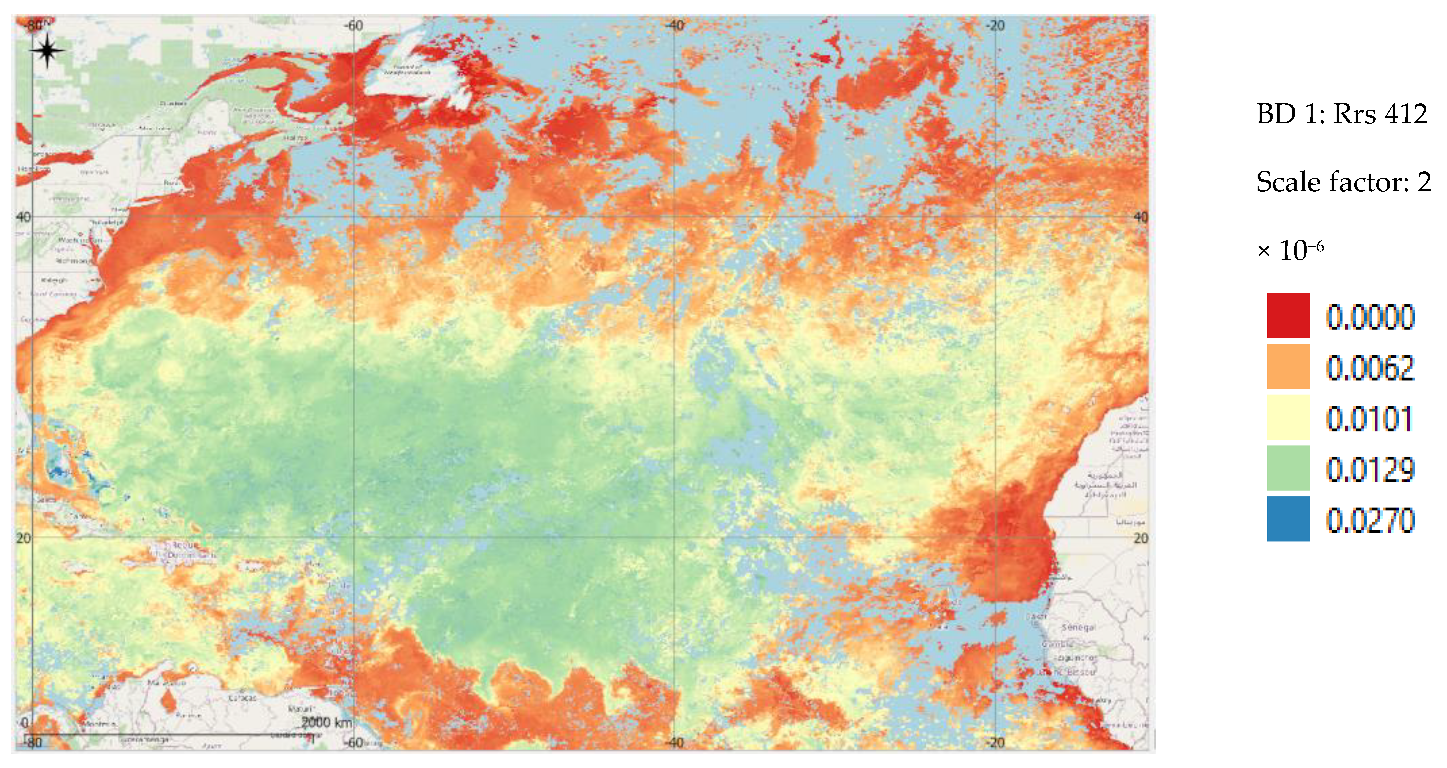
Co-temporal and co-located met-ocean parameters that are considered to be somehow connected with the ocean carbonate system were derived from independent sources using earth observation satellite remote sensing (BD 1–7; PD 1–5), model reanalyses (PD 10), and empirical algorithms (PD 6–8) (Table 2). The GEBCO bathymetry (PD 9) was derived from a mix of ship track soundings, with the interpolation between soundings guided by satellite-derived gravity data.
2.2.3. Justification for the Selection and Use of Environmental Drivers
Figure 2 shows the linkage between the various environmental drivers used in this study and how these were used to model the target ocean surface DIC, TA, and pH. The environmental drivers can be seen to represent the following three proxies of oceanic processes:
- Kinetic forcing, by looking at atmospheric stability (proxies, such as transfer velocity, that affect the partial pressure of CO2 (pCO2), wind speed, wind direction, and wind stress on the ocean surface);
- Thermohaline forcing, by looking at proxies such the sea surface temperature and the sea surface salinity;
- Biological forcing, by looking at proxies such as chlorophyll-a, surface reflectance and its ratios, and particulate organic and inorganic carbon and its ratios;
- Water-side convection and upwelling, by looking at proxies such as mixing layer depth and bathymetry.
These four processes were used to closely represent as much as possible the forcing that leads to the derivation of DIC, TA, and pH using our algorithm. Native resolution grids of all of the environmental drivers considered for this study, including PD1, were resampled to a common 0.04° × 0.04° global raster grid for a suitable retrieval of all co-located data. Table 3 provides a summarized justification for the inclusion of these drivers into the predictive algorithm.
2.3. Algorithm Development and Validation
2.3.1. Training of the ANN
For this study, a back propagation neuron (BPN) algorithm was trained by supervised learning by providing it with values of the co-located and co-temporal environmental drivers (Figure 3) and the corresponding DIC, TA, and pH (Figure 2) that constitute the final output for this study. Since the BPN algorithm is central to much current work on learning in NN, and has been independently invented several times (e.g., [75,76]), we used this algorithm to perform our desired task. The BPN algorithm feeds forward the input training pattern, which is then followed by the back propagation of the associated error, and which is finally expressed as a weight adjustment.
In order to supply training power to the BPN algorithm, the in situ Spring 2016 dataset (i.e., 16–24 April 2016) measurements (Table 1) were used as the values of the output neurons, while their corresponding (i.e., co-located and co-temporal) physico-chemical and biological drivers (Table 2), which were obtained independently, were used as the values of the input neurons. The location of the sampling points spanned across the entire North Atlantic Ocean, and thus presented the desired wide-ranging variability in both the physico-chemical and the biological conditions, which in turn led to the value range of DIC, TA, and pH observed during that period (Table 1). This process was carried out to optimize the BPN weights, such that the error function became minimal. The choice of the input (predictors) and output (predictands) dataset was targeted towards having a BPN algorithm that was able to model the output variables under different physical environmental conditions within the area of interest.
During this algorithm training, the net output was compared with the target value and the resultant error was calculated. It was here that the error factor was distributed back to the hidden layer, and the weights were updated accordingly. The error factor was calculated in a similar manner for all of the units, and their weights were updated simultaneously.
The ultimate objective here was to reduce this training error for the BPN algorithm until the ANN learned on the basis of the training data. The weights were gradually adjusted by means of a learning rule until they were capable of optimizing the predictive modeling of DIC, TA, and pH, as shown in Equation (1), as follows:
f(DIC, TA, pH) = (U10, DD, wind stress, transfer velocity, depth, SSS, chlorophyll-a, SST, Rrs 412, Rrs 443/555, Rrs 531/555, Rrs 443/48, PIC, POC, MLD)
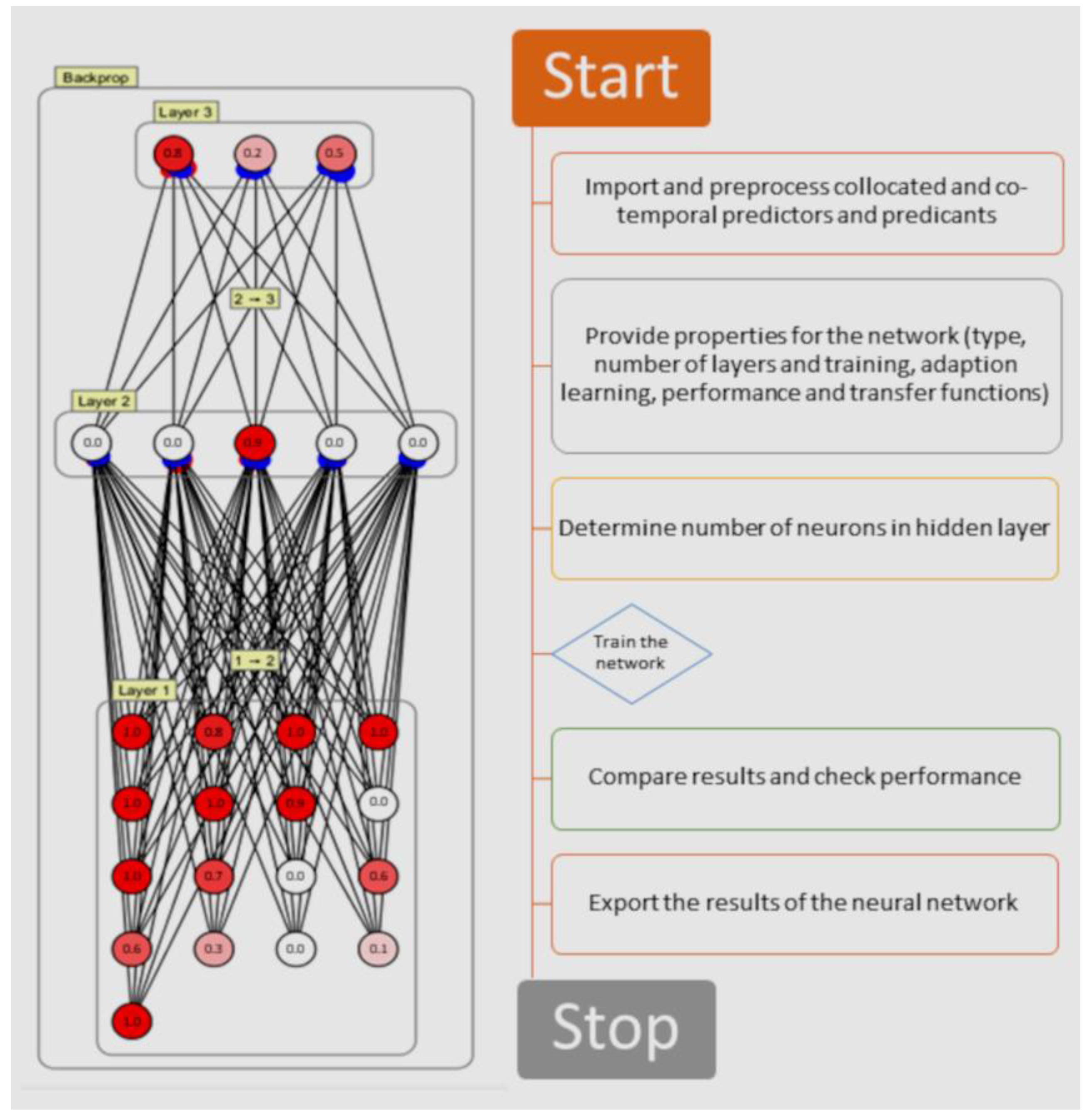
Multi-source, geo-located EO and model reanalysis datasets (Level 4, SMI format) covering the period of 16–24 April 2016 were derived (Figure 3) from the co-located and co-temporal values (corresponding to BD 1–7 and PD 1–10) at the points shown in red (i.e., Spring 2016: ANN training set) in Figure 1. Choosing the right number of hidden neurons is usually performed through trial and error [77]. The ANN optimal topology hinges on the complexity of the relations between inputs and outputs. In this study, two sets of hidden neurons were tested: n = 5 and n = 10, where the assumption was that the greater the number of nodes, the smaller the error on the training set. However, at a certain point, the generalization began to increase, and the first structure (i.e., n = 5) was chosen on the basis of the smallest value for RMSE that was achieved during the training phase. The best topology found in this study consisted of an input layer with 17 neurons, 5 neurons in the hidden layer, and an output layer consisting of 3 neurons whose output gave the scaled DIC, TA, and pH (Figure 4). The training algorithm adjusted the bias and weighting factors according to the negative gradients of the error cost function [58] for the final training pattern.
The ANN training process algorithm for DIC, TA, and pH is shown in Figure 4 as follows:
- The collection of co-located and co-temporal input (i.e., independent environmental drivers) and co-located and co-temporal output (i.e., cruise measurements of DIC, TA, and pH) datasets;
- The data were normalized and scaled to the range of 0 to 1 to suit the transfer function in the hidden (sigmoidal, discrete; logistical implementation) and output layer (linear):  = (A − Amin)/(Amax − Amin), where  is the normalized value and Amin and Amax are the minimum and maximum values of A, respectively;
- Neural network designing and training;
- The testing of the ANN topology.
The training of the BPN algorithm started by using a small, random weight. It propagated each input pattern to the output layer, compared the pattern in the output layer with the correct one, and adjusted the weights according to the back propagation learning algorithm. After the presentation of around 10,000 patterns, the weights converged, i.e., the network picked up the correct pattern, and the error-correction learning stopped. In so doing, the network systematically reduced and/or reinforced the weights of the connection architecture and all of the ‘knowledge’ in the BPN was then contained in the weights. Naturally, the magnitude of this error depended on the choice, relation, quality, and accuracy of the inputs (predictors).
The predictive power of the BPN algorithm was maximized by means of the following steps:
- A large number of iterations was used (circa 10,000) in order to minimize the processing error of the training set as much as possible. The training was stopped when a very small and stable training error was achieved (circa 0.0007);
- The number of learning samples consisted of entire sets of measurements spanning the northwestern Atlantic, with its inherent physical (including bathymetry, surface salinity, winds, wind stress, temperature, and mixed layer depths) and biological (chlorophyll-a, dissolved organic carbon, and surface-leaving reflectance) parameters, in order to model the highest possible scenario for appropriate learning under a wide range of variability. This training procedure can be further improved by including input and output variables with a greater degree of variability, such as measurements covering other regional areas and time periods;
- An optimal number of hidden units (n = 5) was found with the sigmoid activation function and a liner output unit to derive an optimal ‘expressive’ power of the network. The present training set presented a ‘smooth’ function and therefore the number of hidden units needed was kept to a minimum (n = 5). For strongly fluctuating functions, more hidden units are generally needed, which does not seem to be a requirement for our study.
2.3.2. Performance of the BPN Algorithm
Entire M/V Equinox cruise transect datasets were reserved and used as independent datasets to validate the performance of the BPN training method. This is a common practice that ensures that the model can produce reliable estimates outside the range of the learning data (generalization capabilities) [78]. Thus, by assigning the trained BPN algorithm with the values of the fixed set of co-located and co-temporal input neurons as the physico-chemical and biological drivers, the resulting ANN-output-modeled DIC, TA, and pH were validated against the assigned datasets (Table 1).
The precision of the machine learning approach was evaluated, which was based on the trained BPN model, through a comparison with the M/V Equinox dataset using the mean bias (MB; Equation (2)) and the root mean square error (RMSE; Equation (3)), as well as the slope of the linear regression between the ANN-retrieved values and the corresponding in situ measured values, as follows:
where the mean bias is how far the model is from the ground truth data and RMSE determines the error on the test set (or generalization error). The objective of the best BPN model topology was based on the lowest possible metrics for the entire test data.
MB = Σn,i = 1(xi − yi)/n
2.4. Construction of Gridded DIC, TA, and pH Gridded Data for 30 October 2016
Finally, the ability of the trained BPN algorithm to process and generate a huge number of DIC, TA, and pH data points was applied to a 1.1 million km2 subset area located in the mid-North Atlantic Ocean, represented by a total number of 63,360 gridded data points (each encompassing the full set of 17 environmental drivers when available). In view of the extensive retrieval and processing requirements, these data points were based on the validated ANN algorithm and initiated by the physico-chemical and biological drivers that were retrieved on 30 October 2016.
The geographical extent of this area was west −61.00°; east −50.04°; west–east 10.96°; south 24.99°; north 34.96°; and south–north 9.96°. This area was chosen on the basis of its interesting hydrodynamics, as well as on its inter-annual trends in CO2 concentrations. The large temporal and spatial gradients of pCO2, as well as its variability driven by a diversity of physical and biological processes, make the analysis of the carbonate chemistry over the region both interesting and challenging [79]. The study’s region of interest is influenced by the North Atlantic gyre and has a seasonal surface temperature variation of about 8 to 10 °C, occurring alongside a fluctuation in the MLD between the Northern Hemisphere’s winter and summer seasons. On average, the MLD deepens to 200 m in winter up to about 10 m in summer. Generally, nutrients remain below the euphotic zone for most of the year, resulting in low primary production. During winter convective mixing, nutrients penetrate the euphotic zone, causing a short-lived phytoplankton bloom in the spring. All of these seasonal changes ultimately influence the total amount of CO2 in the seawater.
All of the grid-point predictor variables were inserted in the BPN algorithm and the values of DIC, TA, and pH were modeled for that day for the entire area, with a native grid size of 0.04167°. On 30 October, there was a total of 7897 empty grid cells in this area that were attributed to cloud cover and, therefore, the lack of optically retrieved remotely sensed predictors (i.e., chlorophyll-a, Rrs, PIC, and POC).
3. Results and Discussion
3.1. Validation between Remotely Sensed- and Cruise-Derived SST and SSS Data
3.2. Performance of the BPN Algorithm
By means of the independent validation datasets, we evaluated the performance of the algorithm by comparing the BPN-retrieved values of DIC, TA, and pH with the measurements that were taken by M/V Equinox (NCEI Accession 0154382) elsewhere, during the different time periods.
3.2.1. M/V Equinox—7–8 March 2015
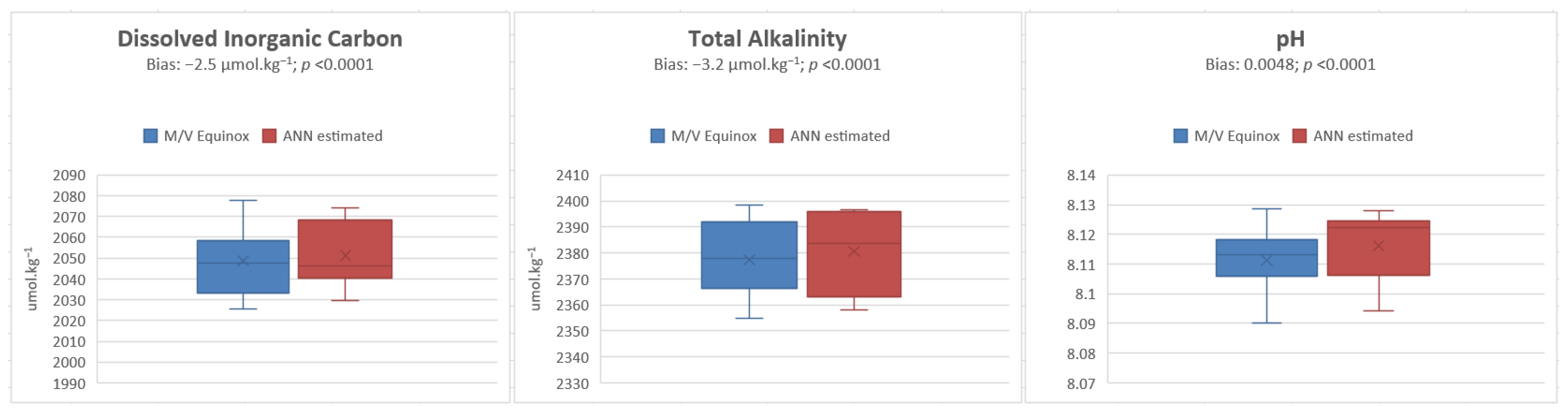
Figure 5 shows the distribution and the statistical significance of the data points within the range that is shown by both in situ and ANN-estimated values, as well as the existence of outliers. The co-located, ANN-estimated DIC, TA, and pH values were in very good agreement with the surface underway measurements given that the BPN algorithm was trained on the data that were collected during 28 April–6 May 2015 along the entire North Atlantic width. The results show that the mean biases for DIC, TA, and pH are −2.5 μmol.kg−1, −3.2 μmol.g−1, and 0.0048, respectively. Compared to the range of DIC, TA, and pH that is shown by the surface underway measurements along all of the transects (Table 1), the values for the mean bias show low variations and a good ANN algorithm performance. Importantly, apart from the fact that no outliers were detected, the overall dispersion of the ANN-estimated values is well within the range of those shown by the M/V data. Some skewness is shown by the ANN-estimated pH and, to a lesser extent, for DIC. The similarity between these three sets of data is statistically significant at the 99% confidence level.
These results point to an effective BPN algorithm that is able to capture the information provided by the chosen environmental drivers. It is important to note that for oceanic and coastal regions with a different matrix of environmental drivers (such as for areas with high chlorophyll-a, where the net productivity is likely to perturb the carbonate system more, or in areas where there are river inputs), further learning of the BPN algorithm is therefore recommended.
3.2.2. M/V Equinox—30 October to 6 November 2016, North Atlantic Ocean (20° N to 40° N; −80° W to −10° W)
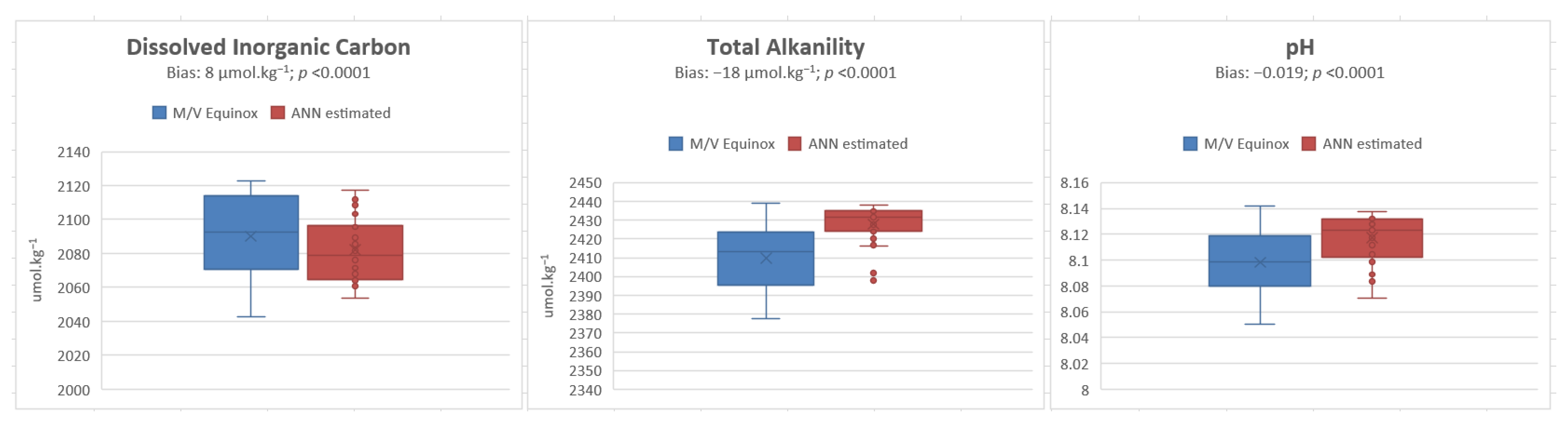
Similarly, Figure 6 shows the resultant statistical evaluation when the ANN-estimated values were compared against the corresponding in situ data. As for the previous validation set, the predictions for the October–November 2016 dataset were in good agreement with the co-located and co-temporal M/V Equinox data. Overall, the ANN-estimated data show less dispersion than the in situ values and that the spread of the former is well within that shown by the data from M/V Equinox. The few ANN-estimated outliers are well within the interquartile range of the M/V Equinox data.
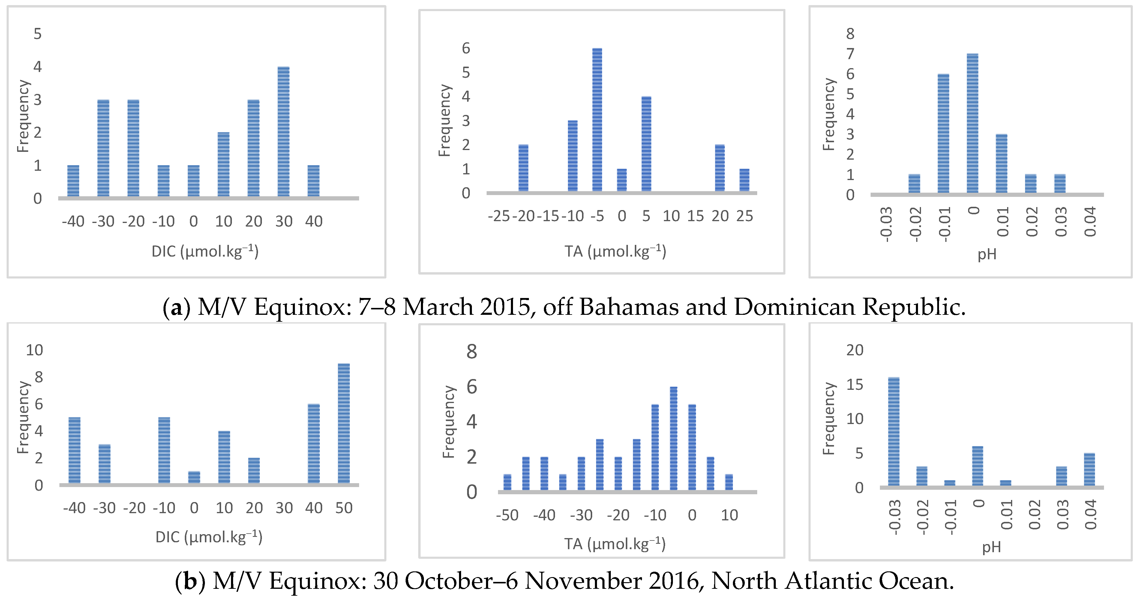
The performance indicators between the modeled and the validation dataset 1 (i.e., the 7–8 March 2015 in situ dataset) point to a stronger estimation than in the case of the second validation dataset. This is most likely because dataset 1 is based on the same seasonal variations of the carbonate chemistry when compared to the second validation sample that was collected during the Autumn of 2016. The mean bias values generally show a non-Gaussian distribution and spread, with the exception of TA for both of the validation datasets, and pH for the Spring 2015 dataset (Figure 7). In the latter case, the residuals are skewed toward lower modeled values.
The uncertainties that were inherent in the in situ measurements were not included in the metadata information within NCEI Accession 0154382, and therefore this element of uncertainty attributed to the surface underway observation could not be evaluated. Overall, however, the results’ metrics are very comparable to the validation metrics that were obtained by Fourrier et al., for their neural network estimation of pH and total alkalinity in the Mediterranean [80]. It is rather complex to identify the main sources of the observed metric errors in view of (1) the procedure that was used by this study and (2) the uncertainty embedded in the in situ data that were used for both the BNP algorithm training and its validation; however, this bias could be expected to decrease if the following steps are taken:
- The further training of the BNP algorithm. In so doing, the training process of the BNP algorithm should allow for further ‘learning’ from the local/regional variability of both the predictors and predictands;
- Although the neural networks have the ability to ‘generalize’, the additional retrieval of in situ measurements of surface DIC, TA, and pH from cruises can be carried out during other seasons over the same area, and combining this with the training set that was used for the BNP algorithm might prove useful;
- Expand the range of predictors (i.e., environmental drivers; see Section 3.3.2 below).
3.3. Model Applications: ANN-Derived Ocean Variability of DIC, TA, and pH over the Mid-North Atlantic Ocean
Based on the previous two validation studies that span different time periods and geographical areas (where each area manifests its own variability in terms of the magnitude of the environmental drivers), we were able to apply the validated ANN topology to model DIC, TA, and pH within the ROI described in Section 2.4 at a resolution of 0.04167°. The final product was a set of gridded, time-specific geophysical maps of these predictands (i.e., surface DIC, TA, and pH). The resolution of these maps took on the native resolution of the input (i.e., predictor) datasets (i.e., 17 environmental drivers). If needed, these raster outputs can be subsequently re-gridded to coarser resolutions in order to (1) further understand the spatiotemporal variability of the carbonate system over specific oceanic regions, (2) comprehensively map the carbonate system components in support of the cruise data, and (3) input the predicted values into numerical modeling systems (such as ocean forecasting models).
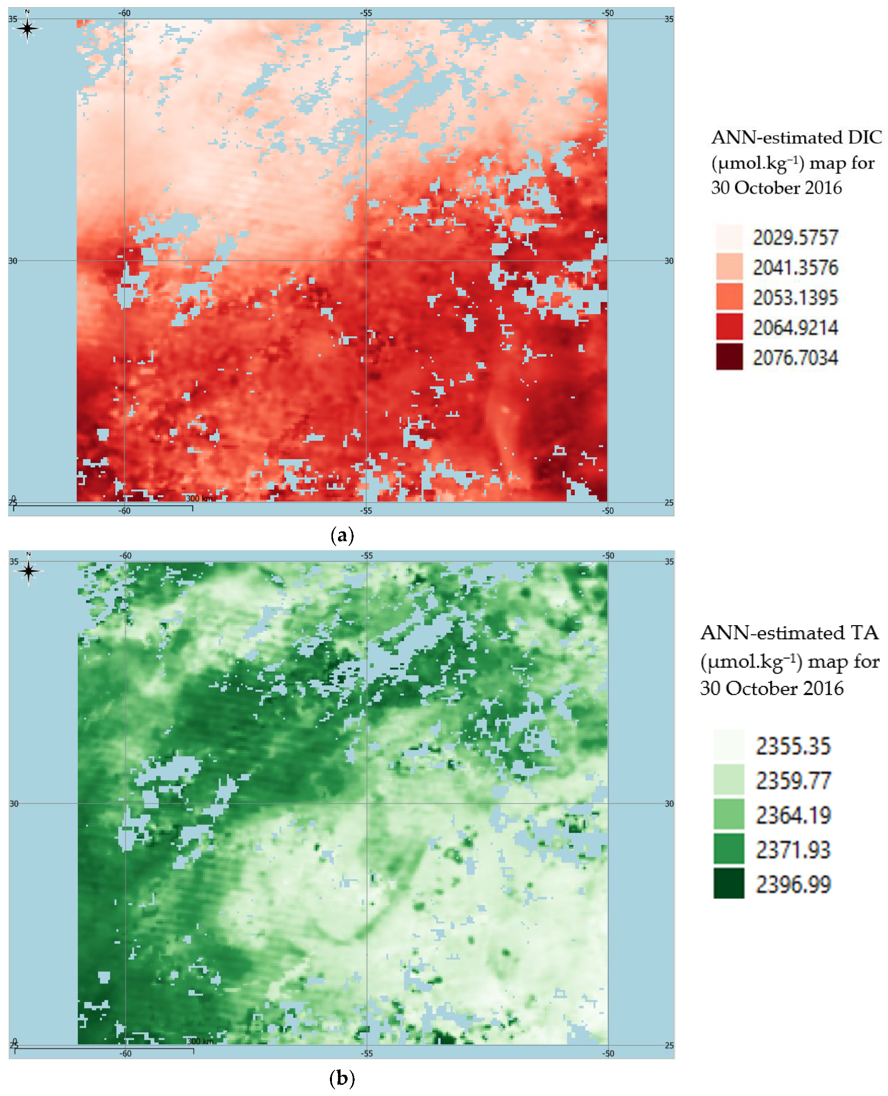
Figure 8a–d represents the gridded output of DIC, TA, and pH maps for the area of interest that were produced by the ANN algorithm. The data gaps represent that no ocean surface data are available whenever clouds obstruct part of the field of view of the optical satellite sensors, at which points the ANN algorithm nullifies the predictions. These high-resolution data representing the carbonate system of the area can be exploited by other modeling activities, including data assimilation for general circulation models [81] and improved model reanalyses [82], as well as the identification of daily trends over sensitive marine areas [83].
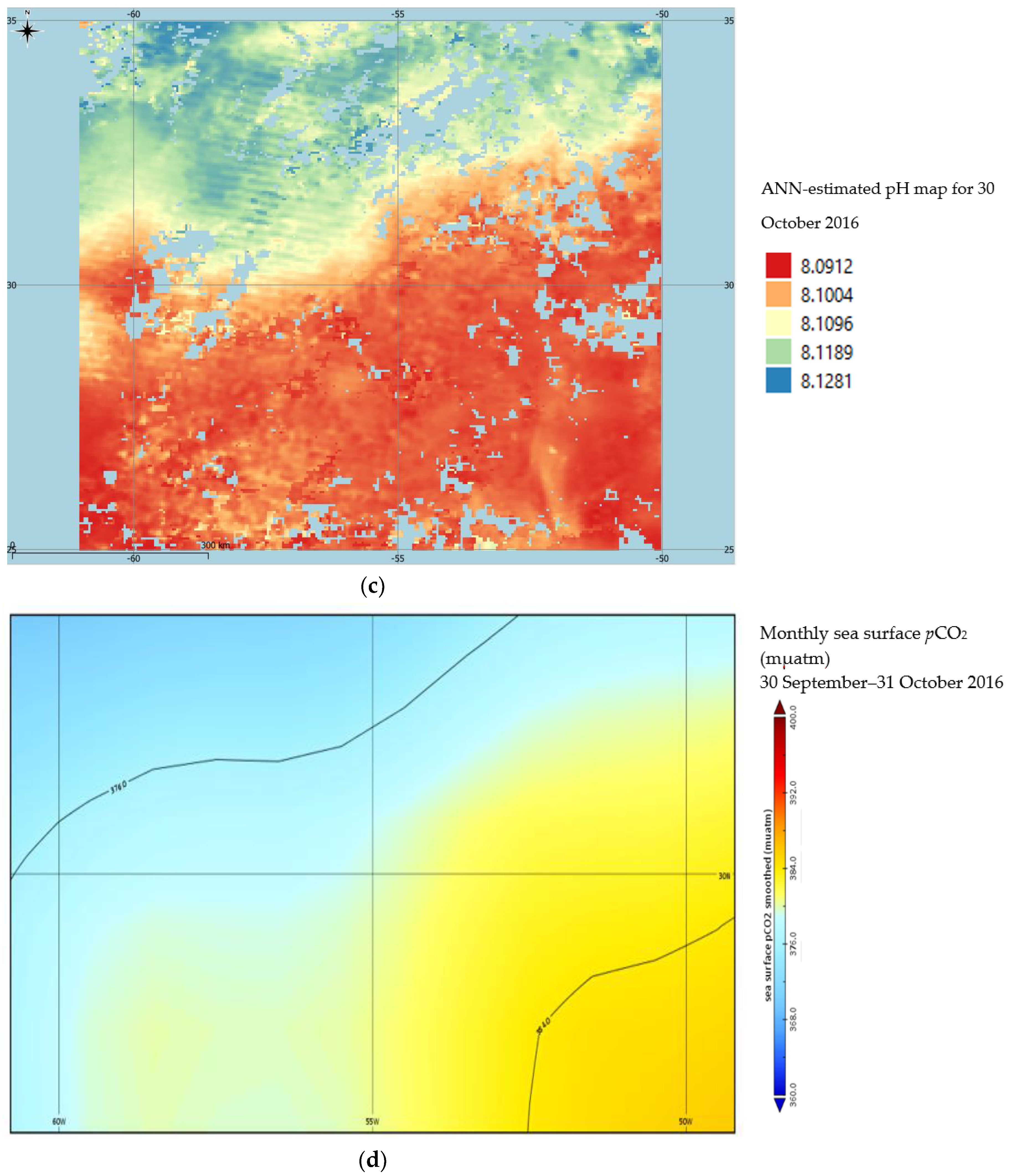
Figure 8d shows how the co-temporal spatial distribution of pCO2 that has been derived by the Landschützer et al., dataset [84] and grid-resampled over our exact area of study is similar to the way that the ANN-estimated pH is distributed. It clearly shows higher pCO2 levels over areas with a lower pH estimate (Figure 8c). This relationship corresponds with the results that were obtained by Sutton et al., (2014) and by Bates et al., (2012) when they studied the variability between pCO2 and pH over the Pacific Ocean and the Atlantic Ocean surface, respectively [19,85]. In our study, the subtle gradient in pCO2 from east to west at around 27° N in Figure 8d is well captured by the modeled spatial variation of the pH high resolution field over the same area (Figure 8c, including the relatively lower pH values corresponding to the northerly pCO2 ‘tongue’ originating from around −58° W, 26° N (Figure 8d).
3.3.1. Validation of the Modeled Data over the Mid-North Atlantic Ocean
- In Situ Cruise Data
The results of the data validation against the in situ datasets available over the same area using validation dataset 3 are shown in Table 5. The in situ cruise transect (comprising StationIDs 1120000–1160000) did not include any pH measurements along the way. The linear regression analysis shows that the correlation between the TA datasets is statistically significant (p < 0.05; 95% C.L.). Moreover, the regressed observations and ANN-estimated DIC and TA values fall within the predicted 95% confidence level of the regression line.
- Hindcast Biochemistry Data
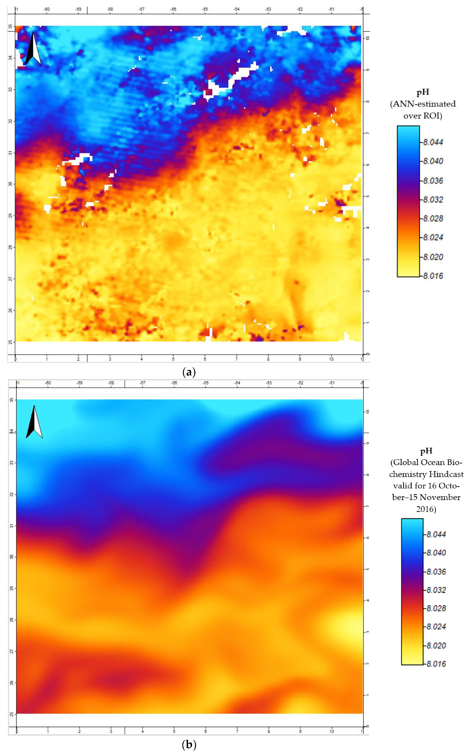
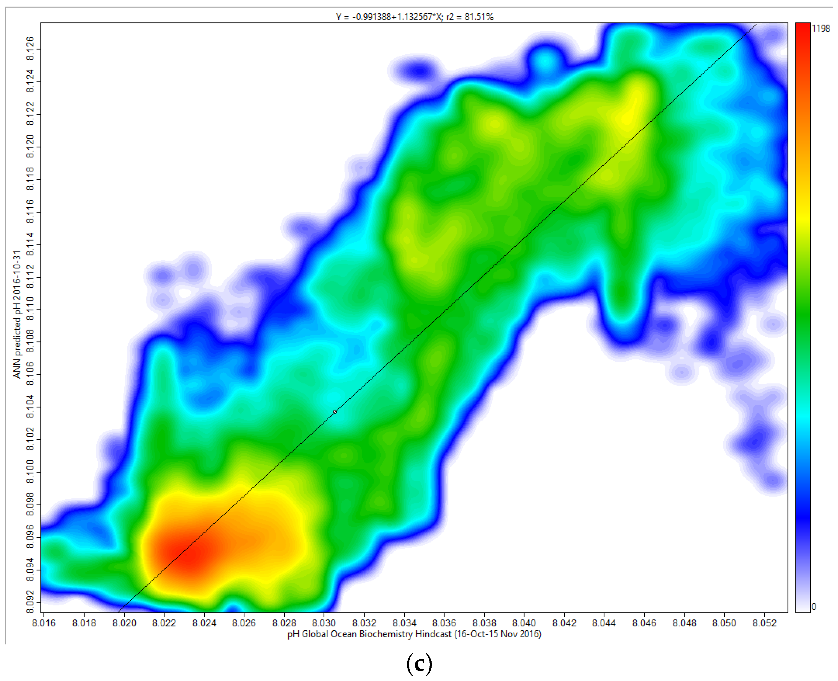
In order to extend the validation of our BPN algorithm, additional independent sources of daily and/or monthly 2016 oceanic surface pH maps were sought; however, this type of dataset proved to be scarce, whilst 2016 daily/monthly gridded oceanic TA and DIC data are non-existent. As of now, the Copernicus Marine Service (CMEMS) makes available the following three datasets: (1) the Global Ocean Biochemistry Hindcast, which consists of both daily and monthly gridded maps (however, the geographic information about pH is only available at a monthly temporal resolution at 0.25° by 0.25° grid resolution); (2) the Global Ocean—in situ reprocessed carbon observations—SOCATv2021, which provides point measurements of DIC, TA, and pH, such as NCEI Accession 0154382; and (3) the Global Ocean Surface Carbon database, which provides pH data on a monthly basis at 1° by 1° grid resolution.
The correlation between the modeled pH (for 30 November 2016) and that derived from the Global Ocean Biochemistry Hindcast (16 October–15 November 2016 at 00:00 h UT) over the area of study is shown in Figure 9. This hindcast database provides monthly data starting as of the 16th day of each month, and therefore this data represents the average value for an entire month. In spite of their slight temporal difference, the two datasets are shown to be strongly correlated together, with an R2 of 0.81 (Figure 9c), indicating a good statistical similarity, as well as an impressive spatial similarity for pH (Figure 9a,b). From an atmosphere–ocean dynamical point of view, this correlation points to a slowly changing pH distribution for the study area over a monthly scale.
3.3.2. Caveats and Recommendations
This study is limited to the estimation of some elements of the carbonate chemistry for the mid-latitude of the North Atlantic Ocean based on their variability during the late winter, spring, and autumn of 2015 and 2016. Whether this neural network algorithm is applicable to other regions of the global oceans and/or for other time periods needs further investigation. The further development and training of the ANN algorithm is therefore recommended. This can be carried out by incorporating (1) a larger scalar variability of the same environmental drivers that are used at the highest spatiotemporal resolution possible in order to improve the learning of the BPN model, and (2) new environmental drivers, such as daily air–sea surface heat fluxes, 2 m air temperature, and air pressure at the highest spatial resolution possible. These may include freshwater influx through precipitation and conditions of the air–sea interface, such as heat fluxes (latent and sensible) and related physical values (such as the sub-layer depth [46]). The atmospheric conditions at sea level are an important parameter that influence the solubility of CO2 in a unit volume of liquid [86]. Increasing the range of EO-based environmental drivers is now becoming more technically feasible, thanks to cloud servers and computing. Equally important would be the derivation of pCO2 as another predictand from our artificial neural network algorithm [87]. Due to the limited time available in obtaining high resolution atmospheric and ocean modeled data, the inclusion of these additional environmental drivers was beyond the scope of the present study. The incorporation of (3) dynamical adjustments made to numerical ocean models [88] on the basis of chosen environmental drivers may further enhance the accuracy of the BPN algorithm. For example, it is necessary to take time-dependent temperature variations into account whenever the wind stress is estimated since it varies by more than a factor of two between 0° and 30 °C because of its dependence on temperature (the Schmidt number).
It is expected that the demand for high resolution DIC, TA, and pH maps, as estimated by deep learning, will, for many reasons, increase in the future. One important use is their support in the monitoring of proposed Ocean Acidification Refugia (OAR), such as the likes of extensive seagrass meadows and dense algal beds [89,90], and algal boundary layers [91,92], slow-flow habitats [93], deep-sea mounts [94], and areas that are isolated from ocean upwelling [95,96]. These are examples of highly localized areas that can vary dramatically across spatial scales from few millimeters (in the case of algal boundary layers) to hundreds of meters squared (such as in the case of extensive seagrass beds), with no clear criteria as to what makes each area a potential OAR other than the observed transient increases in seawater pH relative to the surrounding waters. Kapsenberg and Cyronak (2019) point out the lack of clear, agreed-upon functional criteria for OAR in the context of climate change, which makes it difficult for managers, legislators, and scientists to assess where to invest management efforts [97]. In this regard, this study becomes promising as a way to provide a means by which the daily determination of carbonate chemistry can be made available across multiple spatial scales down to at least a 4 km2 horizontal resolution. In doing so, new target refugia can be proposed for research and management purposes.
4. Conclusions
Changes in ocean carbonate chemistry are a large spatiotemporal scale phenomenon that certainly needs to be monitored at the local scale. This study addresses its first research question by showing a way to produce high resolution, accurate, gridded maps of DIC, TA, and pH that are ideally suited for more localized ocean carbonate studies and applications.
Ship-based sampling remains subjected to limited ship time and human resources, costs, and weather conditions that prevent sampling in specific areas or at certain times of the year. Yet, they remain fundamental for numerical model validation and initialization tasks. This study shows a way to generate very-high-resolution gridded maps of ocean surface DIC, TA, and pH using an ANN approach in a robust and efficient way. This was carried out by addressing the second research question of this study. The future availability of more EO products hosted by cloud-serving computing environments and deep learning will soon be a determining factor towards the future automation of the synthesis of similar, highly detailed, daily carbonate chemistry maps for the global oceans. This technology will definitely help various ocean-related communities to better mitigate and adapt to the expected long-term changes. This is why we feel that high resolution EO products, coupled with deep learning, will provide us with an indirect way to monitor the chemical changes in seawater at an unprecedented resolution.
Author Contributions
Conceptualization, C.G.; Data curation, C.G.; Formal analysis, C.G.; Investigation, C.G.; Methodology, C.G.; Resources, C.G.; Software, C.G.; Validation, C.G.; Visualization, C.G.; Writing—original draft, C.G.; Writing—review and editing, C.G. and R.G. All authors have read and agreed to the published version of the manuscript.
Funding
This research was funded by COST Action CA 15217 Ocean Governance for Sustainability—Challenges, Options, and the Role of Science through short-term scientific missions (STSM) on the ‘Modeling Ocean Acidification in the Gulf of Cadiz (MOsAiGC)’ [CA15217-STSM-39764], and ‘Contemporary Acidification Trends in the coastal NorThEaStern Atlantic (ATlaNTES)’ [CA15217-STSM 40669].
Institutional Review Board Statement
IES-2022-00027. University of Malta.
Informed Consent Statement
Not applicable.
Data Availability Statement
Not applicable.
Acknowledgments
The authors would like to acknowledge Barbero, Leticia, Wanninkhof, Rik, Pierrot, and Denis for the collection of dissolved inorganic carbon, total alkalinity, pH, and other variables collected from surface and discrete observations using a flow-through pump and other instruments from M/V Equinox in the North Atlantic Ocean from 7 March 2015 to 6 November 2016 (NCEI Accession 0154382). The US DOC, NOAA, OAR, and the Atlantic Oceanographic and Meteorological Laboratory are also being acknowledged for hosting and making available this information: https://www.ncei.noaa.gov/access/metadata/landing-page/bin/iso?id=gov.noaa.nodc:0154382 (accessed on 20 February 2023). We would also like to acknowledge COST Action CA 15217 Ocean Governance for Sustainability—Challenges, Options, and the Role of Science—for supporting short-term scientific missions (STSM) on the ‘Modeling Ocean Acidification in the Gulf of Cadiz (MOsAiGC)’ DOI: 10.13140/RG.2.2.32657.99681, and ‘Contemporary Acidification Trends in the coastal NorThEaStern Atlantic (ATlaNTES)’. COST is supported by the EU Framework Program Horizon 2020.
Conflicts of Interest
The authors declare no conflict of interest.
References
- Feely, R.A.; Orr, J.; Fabry, V.J.; Kleypas, J.A.; Sabine, C.L.; Langdon, C. Present and Future Changes in Seawater Chemistry Due to Ocean Acidification. In Carbon Sequestration and Its Role in the Global Carbon Cycle; American Geophysical Union: Washington, DC, USA, 2009; Volume 183, pp. 5–8. [Google Scholar] [CrossRef]
- Bakker, D.C.E.; Pfeil, B.; O’Brien, K.M.; Currie, K.I.; Jones, S.D.; Landa, C.S.; Lauvset, S.K.; Metzl, N.; Munro, D.R.; Nakaoka, S.; et al. Surface Ocean CO2 Atlas (SOCAT) V4. Pangaea 2016. [CrossRef]
- Sabine, C.L.; Hankin, S.; Koyuk, H.; Bakker, D.C.E.; Pfeil, B.; Olsen, A.; Metzl, N.; Kozyr, A.; Fassbender, A.; Manke, A.; et al. Multispectral Remote Sensing Algorithms for Particulate Organic Carbon (POC): The Gulf of Mexico. Remote Sens. Environ. 2009, 113, 50–61. [Google Scholar] [CrossRef] [Green Version]
- Lauvset, S.K.; Lange, N.; Tanhua, T.; Bittig, H.C.; Olsen, A.; Kozyr, A.; Álvarez, M.; Becker, S.; Brown, P.J.; Carter, B.R.; et al. An updated version of the global interior ocean biogeochemical data product, GLODAPv2.2021. Earth Syst. Sci. Data 2021, 13, 5565–5589. [Google Scholar] [CrossRef]
- Tanhua, T.; Orr, J.C.; Lorenzoni, L.; Hansson, L. Monitoring ocean carbon and ocean acidification. WMO Bull. 2015, 64, 48–51. [Google Scholar]
- NRDC. Ocean Acidification Hotspots. Natural Resources Defence Council. 2022. Available online: https://www.nrdc.org/resources/ocean-acidification-hotspots (accessed on 24 September 2022).
- Zeng, J.; Matsunaga, T.; Saigusa, N.; Shirai, T.; Shin-Ichiro, N.; Zheng-Hong, T. Technical note: Evaluation of three machine learning models for surface ocean CO2 mapping. Ocean Sci. 2017, 13, 303–313. [Google Scholar] [CrossRef] [Green Version]
- Jiang, Z.; Song, Z.; Bai, Y.; He, X.; Yu, S.; Zhang, S.; Gong, F. Remote Sensing of Global Sea Surface pH Based on Massive Underway Data and Machine Learning. Remote Sens. 2022, 14, 2366. [Google Scholar] [CrossRef]
- Bittig, H.C.; Steinhoff, T.; Claustre, H.; Fiedler, B.; Williams, N.L.; Sauzède, R.; Körtzinger, A.; Gattuso, J.P. An alternative to static climatologies: Robust estimation of open ocean CO2 variables and nutrient concentrations from T, S, and O2 data using bayesian neural networks. Front. Mar. Sci. 2018, 5, 328. [Google Scholar] [CrossRef]
- Hall, E.R.; Wickes, L.; Burnett, L.E.; Scott, G.I.; Hernandez, D.; Yates, K.K.; Barbero, L.; Reimer, J.J.; Baalousha, M.; Mintz, J.; et al. Acidification in the U.S. Southeast: Causes, Potential Consequences and the Role of the Southeast Ocean and Coastal Acidification Network. Front. Mar. Sci. 2020, 7, 548. [Google Scholar] [CrossRef]
- Ekstrom, J.; Suatoni, L.; Cooley, S.; Pendleton, L.H.; Waldbusser, G.G.; Cinner, J.E.; Ritter, J.; Langdon, C.; Van Hooidonk, R.; Gledhill, D.; et al. Vulnerability and adaptation of US shellfisheries to ocean acidification. Nat. Clim. Change 2015, 5, 207–214. [Google Scholar] [CrossRef]
- Burgos, M.; Sendra, M.; Ortega, T.; Ponce, R.; Gómez-Parra, A.; Forja, J.M. Ocean-Atmosphere CO2 Fluxes in the North Atlantic Subtropical Gyre: Association with Biochemical and Physical Factors during Spring. J. Mar. Sci. Eng. 2015, 3, 891–905. [Google Scholar] [CrossRef]
- Rérolle, V.M.C.; Achterberg, E.P.; Ribas-Ribas, M.; Kitidis, V.; Brown, I.; Bakker, D.C.; Lee, G.A.; Mowlem, M.C. High-resolution pH measurements using a lab-on-chip sensor in surface waters of northwest European shelf seas. Sensors 2018, 18, 2622. [Google Scholar] [CrossRef] [Green Version]
- Palevsky, H.I.; Quay, P.D. Influence of biological carbon export on ocean carbon uptake over the annual cycle across the North Pacific Ocean. Glob. Biogeochem. Cycles 2017, 31, 81–95. [Google Scholar] [CrossRef] [Green Version]
- Liu, M.; Tanhua, T. Water masses in the Atlantic Ocean: Characteristics and distributions. Ocean Sci. 2021, 17, 463–486. [Google Scholar] [CrossRef]
- Vázquez-Rodríguez, M.; Touratier, F.; Lo Monaco, C.; Waugh, D.; Padin, X.A.; Bellerby, R.G.J.; Goyet, C.; Metzl, N.; Ríos, A.F.; Pérez, F.F. Anthropogenic carbon in the Atlantic Ocean: Comparison of four data-based calculation methods. Biogeosciences 2009, 6, 439–451. [Google Scholar] [CrossRef] [Green Version]
- Khatiwala, S.; Tanhua, T.; Mikaloff Fletcher, S.; Gerber, M.; Doney, S.C.; Graven, H.D.; Gruber, N.; McKinley, G.A.; Murata, A.; Ríos, A.F.; et al. Global ocean storage of anthropogenic carbon. Biogeosciences 2013, 10, 2169–2191. [Google Scholar] [CrossRef] [Green Version]
- Lauvset, S.K.; Gruber, N.; Landschützer, P.; Olsen, A.; Tjiputra, J. Trends and drivers in global surface ocean pH over the past 3 decades. Biogeosciences 2015, 12, 1285–1298. [Google Scholar] [CrossRef] [Green Version]
- Bates, N.R.; Best, M.H.P.; Neely, K.; Garley, R.; Dickson, A.G.; Johnson, R.J. Detecting Anthropogenic Carbon Dioxide Uptake and Ocean Acidification in the North Atlantic Ocean. Biogeosciences 2012, 9, 2509–2522. [Google Scholar] [CrossRef] [Green Version]
- NOAA. State of the Climate: Ocean Heat Storage. 2015. Available online: https://www.climate.gov/news-features/featured-images/2015-state-climate-ocean-heat-storage (accessed on 24 September 2022).
- NOAA. Reporting on the State of the Climate in 2016. Available online: https://www.ncei.noaa.gov/news/reporting-state-climate-2016 (accessed on 24 September 2022).
- Clark, D.R.; Flynn, K.J. The Relationship between the Dissolved Inorganic Carbon Concentration and Growth Rate in Marine Phytoplankton. Proc. Biol. Sci. 2000, 267, 953–959. Available online: https://www.jstor.org/stable/1571440 (accessed on 22 August 2022). [CrossRef] [Green Version]
- Barbero, L.; Wanninkhof, R.; Pierrot, D. Dissolved Inorganic Carbon, Total Alkalinity, pH, and Other Variables Collected from Surface and Discrete Observations Using Flow-Through Pump and Other Instruments from M/V Equinox in the North Atlantic Ocean from 2015-03-07 to 2016-11-06 (NCEI Accession 0154382); Dataset; NOAA National Centers for Environmental Information: Washington, DC, USA, 2016. [Google Scholar] [CrossRef]
- Ioannou, I.; Gilerson, A.; Gross, B.; Moshary, F.; Ahmed, S. Deriving ocean color products using neural networks. Remote Sens. Environ. 2013, 134, 78–91. [Google Scholar] [CrossRef]
- Stramska, M. Particulate organic carbon in the global ocean derived from SeaWIFS ocean color. Deep. Sea Res. I 2009, 56, 1459–1470. [Google Scholar] [CrossRef]
- Zhu, Y.; Shang, S.; Shai, W.; Dai, M. Satellite-derived surface water pCO2 and air-sea CO2 fluxes in the northern South China Sea in summer. Prog. Nat. Sci. 2009, 19, 775–779. [Google Scholar] [CrossRef]
- Balch, W.M.; Gordon, H.R.; Bowler, B.C.; Drapeau, D.T.; Booth, E.S. Calcium carbonate budgets in the surface global ocean based on MODIS data. J. Geophys. Res. 2005, 110, C07001. [Google Scholar] [CrossRef]
- Stramski, D.; Reynolds, R.A.; Kahru, M.; Mitchell, B.G. Estimation of particulate organic carbon in the ocean from satellite remote sensing. Science 1999, 285, 239–242. [Google Scholar] [CrossRef] [PubMed]
- Stramska, M.; Stramski, D. Variability of particulate organic carbon concentration in the north polar Atlantic based on ocean color observations with Sea-viewing Wide Field-of-view Sensor (SeaWiFS). J. Geophys. Res. 2005, 110, C10018. [Google Scholar] [CrossRef] [Green Version]
- Boutin, J.; Vergely, J.L.; Marchand, S.; D’Amico, F.; Hasson, A.; Kolodziejczyk, N.; Reul, N.; Reverdin, G.; Vialard, J. New SMOS Sea Surface Salinity with reduced systematic errors and improved variability. Remote Sens. Environ. 2018, 214, 115–134. [Google Scholar] [CrossRef] [Green Version]
- Wanninkhof, R. Relationship between wind speed and gas exchange over the ocean revisted. Limnol. Oceanogr. 2014, 12, 351–362. [Google Scholar] [CrossRef]
- Wanninkhof, R. Relationship between wind speed and gas exchange over the ocean. J. Geophys. Res. 1992, 97, 7373–7382. [Google Scholar] [CrossRef]
- Wanninkhof, R.; McGillis, W.R. A Cubic Relationship between Air-Sea CO2 Exchange and Wind Speed. Geophys. Res. Lett. 1999, 26, 1889–1892. [Google Scholar] [CrossRef]
- Iwano, K.; Takagaki, N.; Kurose, R.; Komori, S. Mass transfer velocity across the breaking air–water interface at extremely high wind speeds. Tellus B Chem. Phys. Meteorol. 2013, 65, 1. [Google Scholar] [CrossRef]
- Hall, J.K. GEBCO centennial special issue—Charting the secret world of the ocean floor: The GEBCO project 1903–2003. Mar. Geophys. Res. 2006, 27, 1–5. [Google Scholar] [CrossRef]
- Dickson, A.G.; Sabine, C.L.; Christian, J.R. Guide to Best Practices for Ocean CO2 Measurements; PICES Special Publication; NOAA: Washington, DC, USA, 2007; Volume 3, pp. 1–191. [Google Scholar]
- Turk, D.; Malacic, V.; De Grandpre, M.D.; McGillis, W.R. Carbon dioxide variability and air-sea fluxes in the northern Adriatic Sea. J. Geophys. Res. 2010, 115, C10. [Google Scholar] [CrossRef] [Green Version]
- Wanninkhof, R.; Asher, W.E.; Ho, D.T.; Sweeney, C.S.; McGillis, W.R. Advances in quantifying air-sea gas exchange and environmental forcing. Ann. Rev. Mar. Sci. 2009, 1, 213–244. [Google Scholar] [CrossRef] [Green Version]
- Macintyre, S.; Wanninkhof, R.; Chanton, J.P. Trace gas exchange across the air-water interface in freshwaters and coastal marine environments. In Biogenic Trace Gasses: Measuring Emissions from Soils and Waters; Mattson, P.A., Harris, R.C., Eds.; Blackwell: New York, NY, USA, 1995; pp. 52–57. [Google Scholar]
- Sweeney, C.; Gloor, E.; Jacobson, A.R.; Key, R.M.; McKinley, G.; Sarmiento, J.L.; Wanninkhof, R. Constraining global air–sea gas exchange for CO2 with recent bomb 14C measurements. Glob. Biogeochem. Cycles 2007, 21, GB2015. [Google Scholar] [CrossRef]
- Ho, D.T.; Law, C.S.; Smith, M.J.; Schlosser, P.; Harvey, M.; Hill, P. Measurements of air-sea gas exchange at high wind speeds in the Southern Ocean: Implications for global parameterizations. Geophys. Res. Lett. 2006, 33, L16611. [Google Scholar] [CrossRef] [Green Version]
- Fairall, C.W.; Hare, J.E.; Edson, J.B.; McGillis, W. Parameterization and Micrometeorological Measurement of Air–Sea Gas Transfer. Bound. Layer Meteorol. 2000, 96, 63–106. [Google Scholar] [CrossRef]
- Krakauer, N.Y.; Randerson, J.T.; Primeau, F.W.; Gruber, N.; Menemenlis, D. Carbon Isotope Evidence for the Latitudinal Distribution and Wind Speed Dependence of the Air–sea Gas Transfer Velocity. Tellus Ser. B Chem. Phys. Meteorol. 2006, 58, 390–417. [Google Scholar] [CrossRef] [Green Version]
- Suzuki, N.; Doneloan, M.A.; Takagaki, N.; Komori, S. Comparison of the global air-sea CO2 gas flux on the difference of transfer velocity model. J. Adv. Mar. Sci. Technol. Soc. 2015, 21, 59–63. [Google Scholar] [CrossRef]
- Boutin, J.; Quilfen, Y.; Merlivat, L.; Piolle, J.F. Global average of air-sea CO2 transfer velocity from QuikSCAT scatterometer wind speeds. J. Geophys. Res. 2009, 114, C04007. [Google Scholar] [CrossRef] [Green Version]
- Woolf, D. Bubbles and their role in gas exchange. In The Sea Surface and Global Change; Liss, P., Duce, R., Eds.; Cambridge University Press: Cambridge, UK, 1997; pp. 173–206. [Google Scholar] [CrossRef]
- Wanninkhof, R.; Knox, M. Chemical enhancement of CO2 exchange in natural waters. Limnol. Oceanogr. 1996, 41, 689–698. [Google Scholar] [CrossRef]
- McGillis, W.R.; Edson, J.B.; Zappa, C.J.; Ware, J.D.; McKenna, S.P.; Terray, E.A.; Hare, J.E.; Fairall, C.W.; Drennan, W.; Donelan, M.; et al. Air-sea CO2 exchange in the equatorial Pacific. J. Geophys. Res. 2004, 109, C08S02. [Google Scholar] [CrossRef] [Green Version]
- Zappa, C.J.; McGillis, W.R.; Raymond, P.A.; Edson, J.B.; Hintsa, E.J.; Zemmelink, H.J.; Dacey, J.W.; Ho, D.T. Environmental turbulent mixing controls on air-water gas exchange in marine and aquatic systems. Geophys. Res. Lett. 2007, 34, 28790. [Google Scholar] [CrossRef] [Green Version]
- Monahan, E.C.; Dam, H.G. Bubbles: An estimate of their role in the global oceanic flux of carbon. J. Geophys. Res. 2001, 106, 9377–9383. [Google Scholar] [CrossRef]
- McNeil, C.; D’Asaro, E. Parameterization of air–sea gas fluxes at extreme wind speeds. J. Mar. Syst. 2007, 66, 110–121. [Google Scholar] [CrossRef]
- Vogelzang, J.; Stoffelen, A.; Verhoef, A.; Figa-Saldaña, J. On the quality of high-resolution scatterometer winds. J. Geophys. Res. 2011, 116, C10033. [Google Scholar] [CrossRef] [Green Version]
- Galdies, C.; Donoghue, D.N.M. A first attempt at assimilating microwave-derived SST to improve the predictive capability of a coupled, high-resolution Eta-POM forecasting system. Int. J. Remote Sens. 2009, 30, 6169–6197. [Google Scholar] [CrossRef]
- Rutgersson, A.; Smedman, A. Enhancement of CO2 transfer velocity due to water-side convection. J. Mar. Syst. 2010, 80, 125–134. [Google Scholar] [CrossRef]
- Brostrom, G. The role of the seasonal cycles for the air–sea exchange of CO2. Mar. Chem. 2000, 72, 151–169. [Google Scholar] [CrossRef]
- Luger, H.; Wallace, D.W.R.; Kortzinger, A.; Nojiri, Y. The pCO2 variability in the midlatitude North Atlantic Ocean during a full annual cycle. Glob. Biochem. Cycles 2004, 18, GB3023. [Google Scholar] [CrossRef] [Green Version]
- Lellouche, J.-M.; Legalloudec, O.; Regnier, C.; Levier, B.; Greiner, E.; Drevillon, M. Quality Information Document for Global Sea Physical Analysis and Forecasting Product 2016. GLOBAL_ANALYSIS_FORECAST_PHY_001_024. Issue 2.0 Provided by the Copernicus Marine Environment Monitoring Service. Available online: https://hpc.niasra.uow.edu.au/dataset/550d2a5a-b66c-4318-aac2-c0fcf64370c0/resource/2d66a089-fe71-47ea-8245-6e1f1d469f59/download/global-analysis-forecast-phy-001-0241551608429013.nc (accessed on 24 September 2022).
- Zeng, J.; Nojiri, Y.; Landschützer, P.; Telszewski, M.; Nakaoka, S. A global surface ocean fCO2 climatology based on a feedforward neural network. J. Atmos. Ocean Technol. 2014, 31, 1838–1849. [Google Scholar] [CrossRef]
- Chen, S.; Hu, C.; Barnes, B.B.; Wanninkhof, R.; Cai, W.-J.; Barbero, L.; Pierrot, D. A machine learning approach to estimate surface ocean pCO2 from satellite measurements. Remote Sens. Environ. 2019, 228, 203–226. [Google Scholar] [CrossRef]
- Cosca, C.E.; Feely, R.A.; Boutin, J.; Etcheto, J.; McPhaden, M.J.; Chavez, F.P.; Strutton, P.G. Seasonal and interannual CO2 fluxes for the central and eastern equatorial Pacific Ocean as determined from fCO2-SST relationships. J. Geophys. Res. 2003, 108, 3278. [Google Scholar] [CrossRef]
- Landschützer, P.; Gruber, N.; Bakker, D.C.E.; Schuster, U.; Nakaoka, S.; Payne, M.R.; Sasse, T.P.; Zeng, J. A neural network-based estimate of the seasonal to inter-annual variability of the Atlantic Ocean carbon sink. Biogeosciences 2013, 10, 7793–7815. [Google Scholar] [CrossRef] [Green Version]
- Takahashi, T.; Olafsson, J.; Goddard, J.; Chipman, D.W.; Sutherland, S.C. Seasonal variation of CO2 and nutrients in the high-latitude surface oceans: A comparative study. Glob. Biogeochem. Cycles 1993, 7, 843–878. [Google Scholar] [CrossRef]
- Hales, B.; Takahashi, T.; Bandstra, L. Atmospheric CO2 uptake by a coastal upwelling system. Glob. Biogeochem. Cycles 2005, 19, GB1009. [Google Scholar] [CrossRef]
- Stephens, M.P.; Samuels, G.; Olson, D.B.; Fine, R.A.; Takahashi, T. Sea-air flux of CO2 in the North Pacific using shipboard and satellite data. J. Geophys. Res. 1995, 100, 13571–13583. [Google Scholar] [CrossRef]
- Ono, T.; Saino, T.; Kurita, N.; Sasaki, K. Basin-scale extrapolation of shipboard pCO2 data by using satellite SST and Chla. Int. J. Remote Sens. 2003, 25, 3803–3815. [Google Scholar] [CrossRef]
- Bates, N.R.; Takahashi, T.; Chipman, D.; Goddard, J.G.; Howse, F.; Knap, A.H. Diurnal to Seasonal Variability of pCO2 in the Sargasso Sea. Variability of PCO2 on Diel to Seasonal Timescales in the Sargasso Sea near Bermuda. J. Geophys. Res. Ocean. 1998, 1031, 15567–15586. [Google Scholar] [CrossRef]
- Watson, A.; Robinson, C.; Robinson, J.; William, P.I.B.; Fasham, M. Spatial variability in the sink for atmospheric carbon dioxide in the North Atlantic. Nature 1991, 350, 50–53. [Google Scholar] [CrossRef]
- Banzon, V.; Smith, T.M.; Chin, T.M.; Liu, C.; Hankins, W. A long-term record of blended satellite and in situ sea-surface temperature for climate monitoring, modeling and environmental studies. Earth Syst. Sci. Data 2016, 8, 165–176. [Google Scholar] [CrossRef] [Green Version]
- NOAA. What Is Upwelling? Available online: https://oceanservice.noaa.gov/facts/upwelling.html (accessed on 24 September 2022).
- Vargas, C.A.; Cuevas, L.A.; Broitman, B.R.; San Martin, V.A.; Lagos, N.A.; Gaitán-Espitia, J.D.; Dupont, S. Upper environmental pCO2 drives sensitivity to ocean acidification in marine invertebrates. Nat. Clim. Change 2022, 12, 200–207. [Google Scholar] [CrossRef]
- Duforêt-Gaurier, L.; Loisel, H.; Dessailly, D.; Nordkvist, K.; Alvain, S. Estimates of particulate organic carbon over the euphotic depth from in situ measurements. Application to satellite data over the global ocean. Deep. Sea Res. Part I Oceanogr. Res. Pap. 2010, 57, 351–367. [Google Scholar] [CrossRef]
- Findlay, H.S.; Calosi, P.; Crawfurda, K. Determinants of the PIC:POC response in the coccolithophore Emiliania huxleyi under future ocean acidification scenarios. Limnol. Oceanogr. 2011, 56, 1168–1178. [Google Scholar] [CrossRef] [Green Version]
- Ridgwell, A.; Schmidt, D.N.; Turley, C.; Brownlee, C.; Maldonado, M.T.; Tortell, P.; Young, J.R. From laboratory manipulations to Earth system models: Scaling calcification impacts of ocean acidification. Biogeosciences 2009, 6, 2611–2623. [Google Scholar] [CrossRef] [Green Version]
- Hu, C.; Lee, Z.; Franz, B. Chlorophyll-a algorithms for oligotrophic oceans: A novel approach based on three-band reflectance difference. J. Geophys. Res. 2012, 117, C01011. [Google Scholar] [CrossRef] [Green Version]
- Bryson, A.E.; Ho, Y.-C. Applied Optimal Control; Blaisdell Publishing Co.: Waltham, MA, USA, 1969. [Google Scholar]
- Rumelhart, D.E.; Hinton, G.E.; Williams, R.J. Learning representations by back-propagating errors. Nature 1986, 323, 533536. [Google Scholar] [CrossRef]
- Svozil, D.; Kvasnicka, V.; Pospichal, J. Introduction to multi-layer feed-forward neural networks. Chemom. Intell. Lab. Syst. 1997, 39, 43–62. [Google Scholar] [CrossRef]
- Bishop, C.M. Neural Networks for Pattern Recognition; Oxford University Press: New York, NY, USA, 1995. [Google Scholar]
- Chau, T.T.T.; Gehlen, M.; Chevallier, F. A seamless ensemble-based reconstruction of surface ocean pCO2 and air–sea CO2 fluxes over the global coastal and open oceans. Biogeosciences 2022, 19, 1087–1109. [Google Scholar] [CrossRef]
- Fourrier, M.; Coppola, L.; Claustre, H.; D’Ortenzio, F.; Sauzède, R.; Gattuso, J.-P. A Regional Neural Network Approach to Estimate Water-Column Nutrient Concentrations and Carbonate System Variables in the Mediterranean Sea: CANYON-MED. Front. Mar. Sci. 2020, 7, 620. [Google Scholar] [CrossRef]
- Campos Velho, H.F.; Furtado, H.C.M.; Sambatti, S.B.M.; Osthoff Ferreira de Barros, C.B.; Welter, M.E.S.; Souto, R.P.; Carvalho, D.; Cardoso, D.O. Data Assimilation by Neural Network for Ocean Circulation: Parallel Implementation. Supercomput. Front. Innov. 2022, 9, 74–86. [Google Scholar] [CrossRef]
- Irrgang, C.; Saynisch-Wagner, J.; Thomas, M. Machine Learning-Based prediction of spatiotemporal uncertainties in global wind velocity reanalyses. J. Adv. Model. Earth Syst. 2020, 12, e2019MS001876. [Google Scholar] [CrossRef] [Green Version]
- United Nations. Ocean Acidification Research on Local Scales. 2022. Available online: https://sdgs.un.org/partnerships/ocean-acidification-research-local-scales (accessed on 24 September 2022).
- Landschützer, P.; Gruber, N.; Bakker, D.C.E. Decadal variations and trends of the global ocean carbon sink. Glob. Biogeochem. Cycles 2016, 30, 1396–1417. [Google Scholar] [CrossRef] [Green Version]
- Sutton, A.J.; Feely, R.A.; Sabine, C.L.; McPhaden, M.J.; Takahashi, T.; Chavez, F.P.; Friederich, G.E.; Mathis, J.T. Natural variability and anthropogenic change in equatorial Pacific surface ocean pCO2 and pH. Glob. Biogeochem. Cycles 2014, 28, 131–145. [Google Scholar] [CrossRef]
- Kraus, E.B.; Businger, J.A. Atmosphere-Ocean Interaction; Oxford University Press: Oxford, UK, 1994; 352p. [Google Scholar]
- Galdies, C.; Garcia-Luque, E.; Guerra, R. Variability CO2 Parameters in the North Atlantic Subtropical Gyre: A Neural Network Approach; Ocean Carbon and Biogeochemistry (OCB) Summer Workshop; Woods Hole Oceanographic Institution: Falmouth, MA, USA, 2018. [Google Scholar]
- Lu, F.; Harrison, M.J.; Rosati, A.; Delworth, T.L.; Yang, X.; Cooke, W.F.; Jia, L.; McHugh, C.; Johnson, N.C.; Bushuk, M.; et al. GFDL’s SPEAR seasonal prediction system: Initialization and ocean tendency adjustment (OTA) for coupled model predictions. J. Adv. Model. Earth Syst. 2020, 12, e2020MS002149. [Google Scholar] [CrossRef]
- Hendriks, I.E.; Olsen, Y.S.; Ramajo, L.; Basso, L.; Steckbauer, A.; Moore, T.S.; Howard, J.; Duarte, C.M. Photosynthetic activity buffers ocean acidification in seagrass meadows. Biogeosciences 2014, 11, 333–346. [Google Scholar] [CrossRef] [Green Version]
- Young, C.S.; Gobler, C.J. The ability of macroalgae to mitigate the negative effects of ocean acidification on four species of North Atlantic bivalve. Biogeosciences 2018, 15, 6167–6183. [Google Scholar] [CrossRef] [Green Version]
- Cornwall, C.E.; Hepburn, C.D.; McGraw, C.M.; Currie, K.I.; Pilditch, C.A.; Hunter, K.A.; Boyd, P.W.; Hurd, C.L. Diurnal fluctuations in seawater pH influence the response of a calcifying macroalga to ocean acidification. Proc. R. Soc. B Biol. Sci. 2013, 280, 20132201. [Google Scholar] [CrossRef] [Green Version]
- Noisette, F.; Hurd, C. Abiotic and biotic interactions in the diffusive boundary layer of kelp blades create a potential refuge from ocean acidification. Funct. Ecol. 2018, 32, 1329–1342. [Google Scholar] [CrossRef] [Green Version]
- Hurd, C.L. Slow-flow habitats as refugia for coastal calcifiers from ocean acidification. J. Phycol. 2015, 51, 599–605. [Google Scholar] [CrossRef]
- Tittensor, D.P.; Baco, A.R.; Hall-Spencer, J.M.; Orr, J.C.; Rogers, A.D. Seamounts as refugia from ocean acidification for cold-water stony corals. Mar. Ecol. 2010, 31, 212–225. [Google Scholar] [CrossRef] [Green Version]
- Chan, F.; Barth, J.A.; Blanchette, C.A.; Byrne, R.H.; Chavez, F.; Cheriton, O.; Feely, R.A.; Friederich, G.; Gaylord, B.; Gouhier, T.; et al. Persistent spatial structuring of coastal ocean acidification in the California Current System. Sci. Rep. 2017, 7, 2526. [Google Scholar] [CrossRef] [Green Version]
- Kapsenberg, L.; Hofmann, G.E. Ocean pH time-series and drivers of variability along the northern Channel Islands, California, USA. Limnol. Oceanogr. 2016, 61, 953–968. [Google Scholar] [CrossRef] [Green Version]
- Kapsenberg, L.; Cyronak, T. Ocean acidification refugia in variable environments. Glob. Change Biol. 2019, 25, 3201–3214. [Google Scholar] [CrossRef] [PubMed] [Green Version]
Figure 1.
Sampling periods of in situ discrete underway samples of DIC, TA, and pH measured by M/V Equinox (source: NCEI Accession 0154382) overlaid over bathymetry (source: GEBCO) for Longitude −80° to −10° and Latitude +18° to +40°. Inset: Winter 2015: Validation dataset 1; Autumn 2016: Validation dataset 2; Spring 2015: Validation dataset 3; Spring 2016: ANN training dataset. The observations along the red transect were used to train the ANN for the prediction of DIC, TA, and pH. The surface underway measurements shown in brown, yellow, and green were used to validate the ANN algorithm against other independent datasets.

Figure 2.
Linkage between the various groups of environmental drivers and how these were used to model or predict the three target parameters of surface DIC, TA, and pH. The environmental drivers can be seen as representing some of the main met-ocean processes influencing these three target variables (based on [38]).

Figure 3.
Multi-source, composite physico-chemical and biological data covering the period of Spring 2016, from which co-located and co-temporal values at points shown in Figure 1 were extracted to train the BPN algorithm. The sources and codes of these multi-source, independent datasets are listed in Table 2.


Figure 4.
The network architecture of the BPN model (left) showing 5 neurons in the hidden layer and the respective weights (in red and blue) of each connection. The values in each of the neurons is a scaled down value (1 decimal place) of the input, hidden, and output neurons, corresponding to one possible solution between the proxy environmental drivers (predictors) and the values for DIC, TA, and pH (predictands). Layer 1 (input): 17 neurons (see Table 1 for a list of input neurons). Layer 2 (hidden): 5 neurons. Layer 3 (output): 3 neurons: DIC, TA, and pH. Steps involved in the development of the BPN model (right).

Figure 5.
Median and variability of ANN-estimated values fall within those shown by discrete underway measurements (Winter 2015 cruise transect). The means of the two datasets are similar at the 99% C.L.
Figure 5.
Median and variability of ANN-estimated values fall within those shown by discrete underway measurements (Winter 2015 cruise transect). The means of the two datasets are similar at the 99% C.L.

Figure 6.
Median and variability of ANN-estimated values fall within those shown by discrete underway measurements (Autumn 2016 cruise transect). The means of the two datasets are similar at the 99% C.L.
Figure 6.
Median and variability of ANN-estimated values fall within those shown by discrete underway measurements (Autumn 2016 cruise transect). The means of the two datasets are similar at the 99% C.L.

Figure 7.
Histogram reporting the distribution of the mean bias values for DIC, TA, and pH.

Figure 8.
Modeled, gridded (a) DIC, (b) TA, and (c) pH maps for the ROI produced by the ANN algorithm. The spatial resolution is 0.04° × 0.04°, which corresponds to the native spatial resolution of some of the predictands. The (d) pCO2 map valid for 30 September until 31 October 2016 has been inserted for reference [78]).


Figure 9.
pH distribution map (a) ANN-estimated pH valid for 30 October 2016; (b) extracted from the Global Ocean Biochemistry Hindcast valid for 16 October–15 November 2016, and (c) scatterplot between (a) and (b) (R2 = 0.81).
Figure 9.
pH distribution map (a) ANN-estimated pH valid for 30 October 2016; (b) extracted from the Global Ocean Biochemistry Hindcast valid for 16 October–15 November 2016, and (c) scatterplot between (a) and (b) (R2 = 0.81).


Table 1.
Data value range and difference Δ along the transects M/V Equinox (ID: MLCE NCEI Accession 0154382) for the entire cruise period.
Table 1.
Data value range and difference Δ along the transects M/V Equinox (ID: MLCE NCEI Accession 0154382) for the entire cruise period.
| Parameter | Range | Δ |
|---|---|---|
| SST (°C) | 15.2–27.5 | 12.3 |
| SSS (PSU) | 35.46–36.95 | 1.49 |
| DIC (μmol.kg−1) | 2025–2126 | 101 |
| TA (μmol.kg−1) | 2350–2439 | 89 |
| pH | 7.964–8.142 | 0.178 |
Table 2.
Co-temporal and co-located environmental drivers derived from independent sources that range from satellite remote sensing and model analyses to empirical algorithms were collected.
Table 2.
Co-temporal and co-located environmental drivers derived from independent sources that range from satellite remote sensing and model analyses to empirical algorithms were collected.
| Parameter | Code | Source | Resolution | Reference |
|---|---|---|---|---|
| Biological drivers | ||||
| Water-leaving surface reflectance (Rrs) at 412, … 555 nm) | BD 1 | MODIS (Aqua, Terra) | 0.042°, daily, global | [24,25] |
| Rrs 443/555 | BD 2 | MODIS (Aqua, Terra) | 0.042°, daily, global | [24,25] |
| Rrs 531/555 | BD 3 | MODIS (Aqua, Terra) | 0.042°, daily, global | [24,25] |
| Rrs 443/488 | BD 4 | MODIS (Aqua, Terra) | 0.042°, daily, global | [24,25] |
| Chlorophyll-a | BD 5 | MODIS (Aqua, Terra) | 0.042°, daily, global | [26] |
| Particulate Inorganic Carbon (PIC) | BD 6 | VIIRS | 0.042°, daily, global | [27] |
| Particulate Organic carbon (POC) | BD 7 | VIIRS | 0.042°, daily, global | [28,29] |
| Physical drivers | ||||
| Sea surface salinity | PD 1 | SMOS | 0.05°, daily, global | [30] |
| Sea surface temperature | PD 2 | OISST | 0.25°, daily, global | [26] |
| Wind speed | PD 3 | ASCAT | 0.25°, daily, global | [26] |
| Wind direction | PD 4 | ASCAT | 0.25°, daily, global | [26] |
| Wind stress | PD 5 | ASCAT | 0.25°, daily, global | [31] |
| Transfer velocity (W) | PD 6 | Based on ASCAT | 0.25°, daily, global | [32] |
| Transfer velocity | PD 7 | Based on ASCAT | 0.25°, daily, global | [33] |
| Transfer velocity | PD 8 | Based on ASCAT | 0.25°, daily, global | [34] |
| Bathymetry | PD 9 | GEBCO | 0.083°, global | [35] |
| Mean layer depth | PD 10 | Global ocean 1/12° physics analysis and forecast updated daily. Copernicus marine environment monitoring service. | 0.083°, daily mean, global analyses, 50 depth levels | [36,37] |
Table 3.
Justification of the use of the biological and physical drivers of surface DIC, TA, and pH used for this study.
Table 3.
Justification of the use of the biological and physical drivers of surface DIC, TA, and pH used for this study.
| Environmental Driver | Summary | Reference |
|---|---|---|
| Transfer velocity | The transfer velocity describes the efficiency exchange of CO2 across the air–sea interface and dissolution in water on the basis of ΔpCO2 between the water and the atmosphere. | [32,33,34,39,40,41,42,43,44,45] |
| Wind speed (U10) and direction (DD) | The wind speed determines the structure and fluxes at the air–sea interface. It has an important effect on the magnitude and direction of the CO2 flux across the air–sea interface, which differs according to the prevalent wind and turbulence regimes. | [46,47,48,49,50,51,52,53] |
| Mean layer depth | This is the depth at which the density difference from the surface reaches 0.02 kg m−3. Within this layer, the properties of density, temperature, and salinity are more uniform, due to the mixing. When this layer is well-defined, a significantly enhanced transfer velocity within it is observed. | [36,37,54,55,56,57] |
| Wind stress | Wind stress is able to affect the vertical transport of dissolved gases, such as CO2. | [31] |
| Sea surface salinity | Sea surface salinity has been used as a proxy indicator for pCO2 using statistical analysis and artificial neural networks. CO2 solubility is a function of temperature and salinity. | [31,58,59,60,61] |
| Sea surfacetemperature | Sea surface pCO2 depends on the SST, such that when the SST increases by 1 °C, the surface pCO2 increases 4-fold. | [26,62,63,64,65,66,67,68] |
| Depth | The depth and structure of the sea bottom can influence the intensity of upwelling. High levels of CO2 from deep water can be brought to the surface through upwelling and released into the atmosphere. This can be enhanced in the case of an existing deep-water circulation. | [69] |
| Biological activity | Photosynthesis acts to bind CO2 into organic matter and can affect DIC concentration. Studies show that chlorophyll-a correlates well with pCO2. | [26,67,70] |
| Particulate Organic carbon (POC) | POC is a proxy of coccolithophore production, which in turn is often used as a measure of net productivity. The phenomenon of sinking POC is part of the biological pump, which provides a mechanism for the sequestration of carbon in the deep ocean. | [25,71] |
| Particulate Inorganic Carbon (PIC) | PIC is used as a measure of net calcification by coccolithophores. The PIC:POC ratio is considered to be an important term for modeling carbon cycling in the oceans and, therefore, is a good indicator of changes in seawater CO2. | [72,73,74] |
Table 4.
Correlation between same variables obtained remotely and by M/V Equinox [ID: MLCE; 7 March 2015 to 6 November 2016] cruise-segmented datasets. Their p-value is <0.00001 and all of the correlations are significant at p < 0.05.
Table 4.
Correlation between same variables obtained remotely and by M/V Equinox [ID: MLCE; 7 March 2015 to 6 November 2016] cruise-segmented datasets. Their p-value is <0.00001 and all of the correlations are significant at p < 0.05.
| Sampling Period | Pearson Correlation R–Sea Surface Temperature | Pearson Correlation R–Sea Surface Salinity |
|---|---|---|
| 7–8 March 2015 | 0.78 | 0.93 |
| 28 April–6 May 2015 | 0.99 | 0.69 |
| 16–24 April 2016 | 0.98 | 0.90 |
Table 5.
Corresponding ship-based and ANN-estimated values for DIC, TA, and pH. In situ pH measurements were not collected by M/V Equinox during part of the transect of 28 April–6 May 2015 (Validation dataset 3). (n/a: not available). The location of the individual StationIDs is as follows: 1120000: (31.1390° N, −60.5765° W); 1130000: (31.3795° N, −59.3347° W); 1140000: (31.7085° N, −57.6472° W); 1150000: (32.1818° N, −55.2020° W); 1160000: (32.7458° N, −52.2730° W); 1200000: (34.0460° N, −45.4433° W); and 1330000: (27.5105° N, −78.8207° W).
| Discrete Underway Measurements | ANN Estimation | Mean Bias | |||||||
|---|---|---|---|---|---|---|---|---|---|
| StationID | DIC (μmol·kg−1) | TA (μmol·kg−1) | pH | DIC (μmol·kg−1) | TA (μmol·kg−1) | pH | TA (μmol·kg−1) | DIC (μmol·kg−1) | pH |
| 1120000 | 2074 | 2387 | n/a | 2064 | 2385 | 8.111 | 10 | 2 | n/a |
| 1130000 | 2078 | 2397 | n/a | 2066 | 2378 | 8.105 | 12 | 19 | n/a |
| 1140000 | 2076 | 2404 | n/a | 2071 | 2368 | 8.099 | 5 | 36 | n/a |
| 1150000 | 2081 | 2400 | n/a | 2066 | 2375 | 8.104 | 15 | 25 | n/a |
| 1160000 | 2083 | 2392 | n/a | 2062 | 2384 | 8.112 | 21 | 7 | n/a |
| 1200000 | 2078 | 2382 | 8.073 | 2075 | 2378 | 8.096 | 3 | 4 | −0.023 |
| 1330000 | 2095 | 2390 | 8.073 | 2073 | 2388 | 8.099 | 21 | 1 | −0.025 |
Disclaimer/Publisher’s Note: The statements, opinions and data contained in all publications are solely those of the individual author(s) and contributor(s) and not of MDPI and/or the editor(s). MDPI and/or the editor(s) disclaim responsibility for any injury to people or property resulting from any ideas, methods, instructions or products referred to in the content. |
© 2023 by the authors. Licensee MDPI, Basel, Switzerland. This article is an open access article distributed under the terms and conditions of the Creative Commons Attribution (CC BY) license (https://creativecommons.org/licenses/by/4.0/).
Share and Cite
MDPI and ACS Style
Galdies, C.; Guerra, R. High Resolution Estimation of Ocean Dissolved Inorganic Carbon, Total Alkalinity and pH Based on Deep Learning. Water 2023, 15, 1454. https://doi.org/10.3390/w15081454
AMA Style
Galdies C, Guerra R. High Resolution Estimation of Ocean Dissolved Inorganic Carbon, Total Alkalinity and pH Based on Deep Learning. Water. 2023; 15(8):1454. https://doi.org/10.3390/w15081454
Chicago/Turabian StyleGaldies, Charles, and Roberta Guerra. 2023. "High Resolution Estimation of Ocean Dissolved Inorganic Carbon, Total Alkalinity and pH Based on Deep Learning" Water 15, no. 8: 1454. https://doi.org/10.3390/w15081454
Note that from the first issue of 2016, this journal uses article numbers instead of page numbers. See further details here.