
Performance of Frequency-Corrected Precipitation in Ungauged High Mountain Hydrological Simulation

1
Northwest Institute of Eco-Environment and Resources, Chinese Academy of Sciences, Lanzhou 730000, China
2
State Key Laboratory of Hydraulics and Mountain River Engineering, College of Water Resource and Hydropower, Sichuan University, Chengdu 610065, China
3
Institute of Desert Meteorology, China Meteorological Administration, Urumqi 830002, China
*
Author to whom correspondence should be addressed.
Water 2023, 15(8), 1461; https://doi.org/10.3390/w15081461
Submission received: 10 March 2023
/
Revised: 31 March 2023
/
Accepted: 6 April 2023
/
Published: 8 April 2023
(This article belongs to the Special Issue The Role of Snow in High-Mountain Hydrologic Cycle)
Abstract
:Accurate precipitation data are essential for understanding hydrological processes in high mountainous regions with limited observations and highly variable precipitation events. While frequency-corrected precipitation data are expected to aid in understanding hydrological processes, its performance in ungauged high mountain hydrological simulation remains unclear. To clarify this issue, we conducted a numerical experiment that used reanalysis precipitation, frequency-corrected precipitation, and gridded precipitation to drive a distributed cold region hydrological model. We selected an ungauged basin in high mountain Asia (Manas River Basin in China) as the study area and employed a statistical parameter optimization method to avoid subjectivity in parameter selection. Our findings indicate that the frequency information from the few existing stations can aid in correcting the reanalysis precipitation data. The frequency correction approach can reduce the total volume of errors in the reanalysis precipitation data, especially when severe biases occur. Our findings show that frequency-corrected precipitation performs better in modeling discharge, runoff depth, and evaporation. Furthermore, the improvement in precipitation using frequency correction bears clear altitude differences, which implies that having more stations at different altitudes is necessary to measure precipitation accurately in similar areas. Our study provides a feasible flow for future precipitation preparation for similar ungauged high mountain areas. Frequency correction, instead of direct interpolation, may be a viable option for precipitation preparation. Our work has reference implications for future hydrological simulations in similar ungauged high mountains.
1. Introduction
Accurate precipitation data are essential for understanding the hydrological processes in high mountainous regions [1], where the precipitation data contain significant uncertainties due to scarce observation and high heterogeneity in precipitation events [2]. Some studies suggest that mountain precipitation is frequently underestimated [1,3], while other studies propose the opposite opinion based on different data sources [4]. This precipitation uncertainty leads to a lack of understanding of hydrological processes in high mountainous areas [5].
In situ observation has long been regarded as the most reliable means for obtaining accurate precipitation data. Although intensive in situ precipitation observation can improve the performance of hydrological modeling in high mountain catchments [6], most meteorological stations are located in the lower altitudes in the high Asian mountainous region, which makes the gridded precipitation from the meteorological stations difficult to reflect the real precipitation distribution of complex mountainous areas. On the other hand, remote sensing precipitation data bear a wide observation range to cover impenetrable mountains, and some of them have a high spatial resolution. An obstacle to using remotely sensed precipitation data is that they are easily affected by system errors and are insensitive to trace precipitation [7,8]. In addition to remote sensing precipitation data, reanalyzed or assimilated precipitation data based on general circulation model (GCM) and regional climate models (RCM) are also usually employed because of their stability and robustness, such as European Centre for Medium-Range Weather Forecasts (ECMWF) Re-Analysis (ERA) series of data [9], the Japanese 55-year Reanalysis (JRA-55) [10], the National Centers for Environmental Prediction (NCEP) Climate Forecast System Reanalysis (NCEP-CFSR) [11], NCAR Global Climate Four-Dimensional Data Assimilation (CFDDA [12] and High Asia Refined analysis (HAR) [13]. Some studies have proved that high-resolution atmospheric models can better reproduce precipitation than gridded data from observational networks in mountains [14]. Irrespective of whether the data are from remote sensing precipitation or reanalyzed precipitation, all have noticeable biases [15,16]. They need to be corrected using different bias-correction methods.
Different correction methods for spatially distributed precipitation include total volume correction and frequency correction. The total volume correction, such as the delta change (DC) approach [17] and the linear-scaling (LS) approach [18], can adjust the total and mean volume of the precipitation, but is less effective in revising extreme precipitation [19]. Relative to the total volume correction, the frequency correction method not only corrects the frequency distribution of precipitation intensities but also the total precipitation. The frequency correction (matching) method is one of the most important methods in precipitation correction [20]. Quantile Mapping (QM) is a typical frequency correction method with advantages in non-parameter error correction and can correct the frequency distribution of precipitation [21]. This method assumes precipitation has a relatively stable probability distribution function over a long time series, and the probability distribution of simulated precipitation should follow the probability distribution of observed precipitation. Previous studies have indicated that applying quantile mapping to temporal subsamples of data can improve the bias correction of daily precipitation [22]. Researchers in Zhang et al. [23] also suggested that the QM method can improve bias correction of global climate model daily precipitation. Ref. Cannon et al. [21] found that the quantile delta mapping algorithm can preserve relative changes in precipitation quantiles. The authors of Heo et al. [24] suggested that two-shape parameter distribution models are more effective than conventional distributions in the quantile mapping method for bias correction of precipitation data. Overall, the QM method is currently the mainstream method for precipitation correction, which can correct the mean precipitation and the variability and frequency distribution of precipitation. Since frequency-corrected precipitation can better describe the intensity and distribution, it is expected to help understand the hydrological processes in high mountain areas.
As mentioned above, the performance of frequency-corrected precipitation in ungauged high mountain hydrological simulation remains unclear. The major challenges can be summarized as follows: (1) Most current evaluations focus on existing precipitation data in simulating the discharges [25,26], but not the effect of frequency correction in hydrological simulation, especially in the change of simulated flow frequency. In addition, previous studies do not clarify the influence of frequency-corrected precipitation on simulated evaporation. (2) Although some studies have suggested that the hydrological simulated streamflow and evaporation can be used to evaluate precipitation forcing [27], there is still some confusion on how to use the hydrological model in these evaluations, especially on how the hydrological parameters should be set in a manner where they can be adjusted corresponding to different precipitation inputs. (3) The ungauged high mountain areas have few station observations, leading to considerable uncertainties in frequency correction results. This may limit the application of frequency-corrected precipitation in these regions. However, on the other hand, it also raises an interesting question of whether the frequency-corrected precipitation could improve the performance of hydrological simulation in these ungauged areas.
Aimed at tackling the above challenges, we designed a numerical experiment to examine the performance of hydrological simulation in ungauged high mountain areas using the frequency-corrected reanalysis precipitation datasets. These objectives include: (1) To evaluate the three precipitation datasets at station and basin scales.(2) To examine the performance of frequency-corrected precipitation in simulating the discharges. The reanalysis and gridded precipitation from the limited meteorological stations were also used to drive the cold region hydrological model. The simulated discharges and evaporation from three precipitation datasets were compared. (3) To evaluate the advantages of the frequency-corrected precipitation in hydrological simulation with the comparison results.
2. Methodology
2.1. Design of Experiments
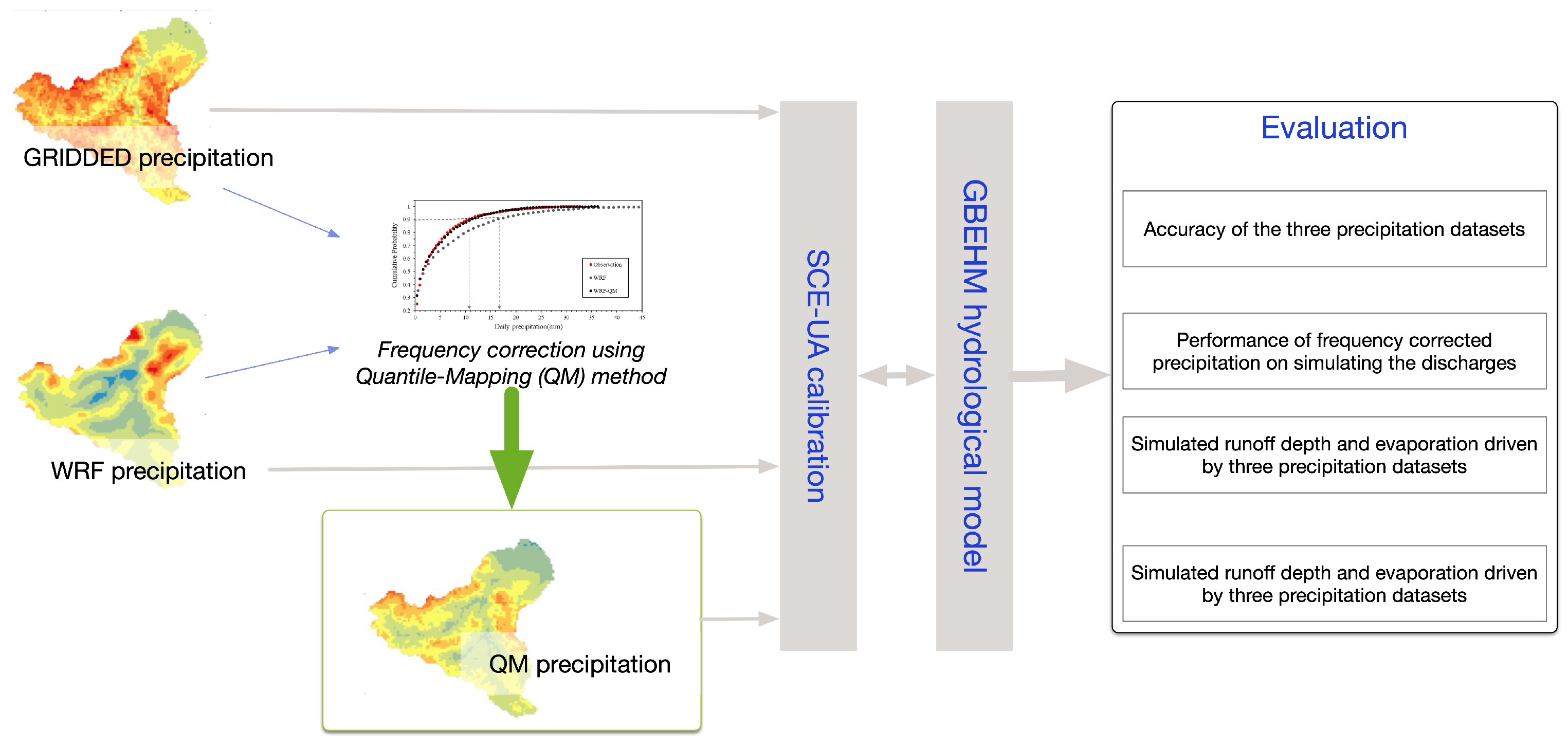
We aimed to evaluate the performance of frequency-corrected precipitation in simulating the hydrological cycle in ungauged high mountain areas. To accomplish this goal, we utilized a distributed cold region hydrological model to assess the hydrological simulation performance of three precipitation datasets: the GRIDDED precipitation, downscaled precipitation using the Weather Research and Forecasting (WRF) Model, and frequency-corrected precipitation (Figure 1).
To evaluate and compare the simulated discharge, evaporation, and inputted precipitation for the three datasets, we employed a statistical parameter optimization method to calibrate the model parameters, thus avoiding the influence of the artificial choice of model parameters. The optimization method’s role is to assess and prove the performance of the frequency-corrected reanalysis precipitation datasets.
We selected an ungauged high mountain basin in High Mountain Asia with only a few stations around the basin. We created three precipitation datasets for comparison purposes: the first is the gridded precipitation interpolated from the existing few station observations, the second is downscaled precipitation from the Weather Research and Forecasting (WRF) Model to represent the reanalysis precipitation, and the third is frequency-corrected precipitation based on the WRF precipitation. The WRF precipitation data were frequency corrected using the Quantile-Mapping method as introduced in Section 2.3.3.
For the reader’s convenience, we have included a list of abbreviations at the end of the article.
2.2. Study Area and In Situ Data
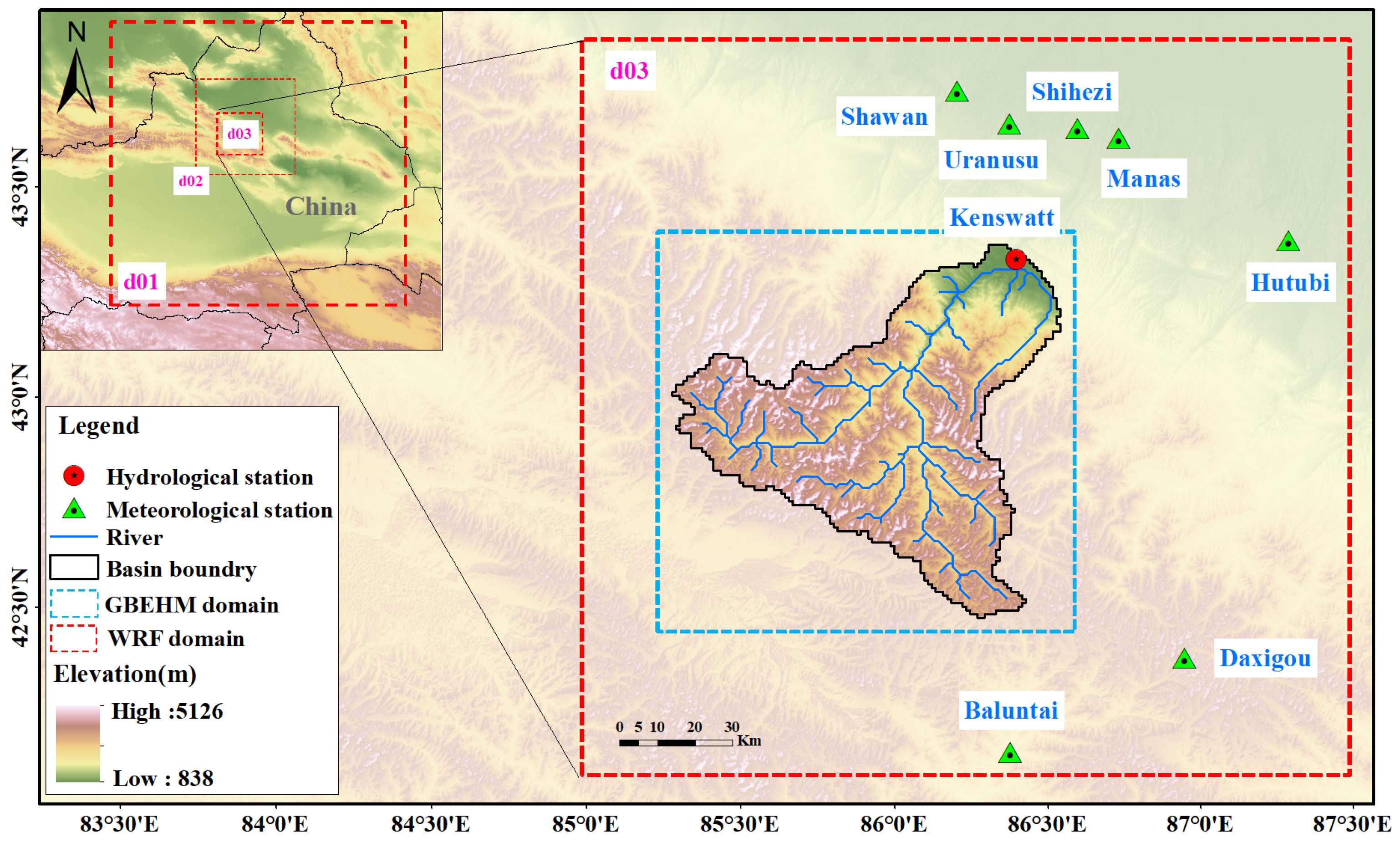
The Manas River Basin in China was selected as the study area, with a latitude and longitude range of 84.9°–86.2° E and 43.0°–44.0° N, covering an area of about 5156 km² (with Kenswat station as the basin outlet) (Figure 2). The basin is located in northwestern High Mountain Asia. The basin’s topography shows a trend of high in the south and low in the north, with elevations ranging from 875 m to 4875 m. The Manas River, the largest inland river in the Junggar Basin, originates from the glaciers and snow mountains in the middle section of the northern Tianshan Mountains. Precipitation is the Manas River basin’s primary water resource, with annual precipitation reaching 500 mm. Still, due to the influence of topography, precipitation is highly unevenly distributed, reaching 600–1000 mm in the river source area and only 100–200 mm in the mountain front [28].
The Manas river basin is a typical ungauged area without precipitation observation. There are seven meteorological stations around the north and south fringe of the basin and a hydrological station (Kenswat station) at the outlet. We selected the precipitation data from these stations as the in situ observation in frequency correction.
2.3. Frequency Correction of Precipitation Data
2.3.1. The GRIDDED Precipitation
This study used an improved three-dimensional thin plate spline (3DTPS) method to interpolate the monthly precipitation at 1 km resolution [29]. This interpolation method considers the effect of elevation on precipitation and uses altitude as a covariate for interpolation. In situ precipitation observations from the seven stations outside of the basin were chosen for the interpolation. The daily precipitation ratio is interpolated using the Ordinary Kriging method based on the monthly precipitation interpolation results. In this study, we choose an isotropic exponential variogram model to fit the semi-variance function for generating the GRIDDED daily precipitation ratio. Finally, the daily precipitation ratio is multiplied by the monthly precipitation to obtain the daily GRIDDED precipitation data with a 1 km resolution.
2.3.2. The WRF Precipitation
We used the ERA-interim reanalysis data as the initial and boundary fields, which are downscaled using the WRF model to obtain the study area’s meteorological forcing data, including precipitation. This study selected the ERA-interim reanalysis data for the Manas River basin from 2004 to 2009 with a temporal resolution of 6 hours and a spatial resolution of 0.25°. The WRF downscaling simulation uses a three-layer nesting scheme, with a resolution of 30 km for the outermost layer, 10 km for the middle layer, and 3.3 km for the innermost layer (Figure 2), with a temporal resolution of 1 h. The WRF model was run from 1 December 2003, to 31 December 2009, with 1 December 2003, to 1 January 2004, as the model warm-up period. In addition to precipitation, the final outputs for the hydrological simulation include long-wave radiation, surface atmospheric pressure, short-wave radiation, 2 m height air temperature, 10 m wind speed, and 2 m humidity. These outputted variables with 3.3 km resolution were then spatially interpolated to the 1 km grid to drive the hydrological model.
2.3.3. The QM Precipitation
The frequency correction method for precipitation is the Quantile-Mapping (QM) method [30]. The WRF precipitation data were frequency corrected using the Quantile-Mapping method which considers the observed and the simulated precipitation identical in the frequency distribution. Aside from the WRF precipitation, any other reanalysis precipitation data could be frequency corrected using the same flow.
This method revises the simulated precipitation by establishing a transfer function between two precipitation datasets (the target precipitation dataset and the precipitation dataset to be corrected).
The transfer function (TF) can be formulated as,
where is the corrected precipitation at the i interval, being assumed the same with the frequency distribution of the target precipitation dataset (here we use the GRIDDED precipitation). is the WRF precipitation to be corrected at the i interval.
This study establishes the transfer function based on the segmental fitting method. The frequency distribution from the GRIDDED precipitation was regarded as the reference and used to revise the frequency of the WRF precipitation grid-by-grid.
First, the cumulative distribution function is calculated and then a piecewise function is used to avoid over-correction [31]. In this method, the daily WRF and GRIDDED precipitation are sorted in ascending order. The precipitation days with daily precipitation greater than 0.1 mm are considered effective precipitation days, and the remaining precipitation events are divided into 100 intervals. These intervals are divided into >98%, <95%, and (95–98%) according to their precipitation values. For each part, a different linear fitting revision factor is used so that the revised cumulative distribution function is the same as the observed value. The transfer function can be written as,
where x is the WRF precipitation to be corrected, and are the correction coefficients for each interval. The correction coefficients are different from each grid of the basin.
2.4. Hydrological Simulation for Checking the Performance of Different Precipitation Datasets
This paper uses the Geomorphology-Based Eco-Hydrological Model (GBEHM) to simulate hydrological processes for the GRIDDED, WRF, and QM precipitation. The GBEHM is a distributed cold region model that uses a flexible distributed scheme to represent the basin topography, takes the flow zone as the basic unit, which can reasonably simulate the discharges in mountainous watersheds [32]. The model includes three typical cryosphere modules: glacier module [33], snow module [34], and frozen soil module [33]. These modules were built based on the water and heat balance method. The GBEHM model has been widely used in high mountain areas [35,36].
The forcing data for the GBEHM are from the WRF model, which has been introduced in Section 2.3.2. The parameters used in the model are listed in Table 1.
To avoid the influence of the artificial choice of model parameters, the SCE-UA global optimization method [40] was used to calibrate the parameters of the GBEHM model. The calibration period spans from 2004 to 2006, and the validation period is from 2007 to 2009.
The Shuffled Complex Evolution (SCE-UA) algorithm is a global optimization algorithm. It was initially developed to calibrate conceptual rainfall-runoff models [40] and has since found widespread applications across a diverse range of science and engineering fields [41]. The algorithm has been benchmarked against other optimization algorithms and has been found to be effective in exploring different regions of a search space, avoiding local optima, converging towards the global optimum, and exploiting promising regions of a search space during optimization effectively [42]. For better computational efficiency, researchers have developed parallel versions of the algorithm [43,44]. Here, we used the version restructured and parallelized by the authors in Houska et al. [43].
The SCE-UA algorithm’s parameters include the number of points in a complex, the number of points in a subcomplex, the number of consecutive offspring generated by each subcomplex, the number of evolution steps taken by each complex, the number of complexes, and the number of past evolution loops. We adopted the default values for the first four parameters, as suggested by Duan et al. [40]. For the number of complexes, we have set it to seven, which is greater than the number of analyzed six parameters in our study, as recommended by Duan et al. [40]. The number of past evolution loops is set to 50.
The SCE-UA algorithm used in this study automatically calibrates the hydrological model with three precipitation datasets, provides a relatively fair evaluation of the hydrological simulation capacity for the three precipitation datasets, and avoids subjectivity in parameter selection as much as possible. We acknowledge that the SCE-UA parameters do introduce some uncertainties, but these uncertainties would equally influence the three cases in our study.
2.5. Accuracy Measures
The root-mean-square error (), Nash–Sutcliffe efficiency coefficient (), and the volume difference () were used to evaluate the model performance in simulating the discharges. The root-mean-square error () and the total volume bias () were used to measure the precipitation error before and after the calibration.
These measures could be formulated as,
where is the mean of the observed variables (precipitation or discharge), denotes the modeled discharges or the corrected precipitation, and represents the observed variables at time t, and represent the precipitation before and after the correction at the day. n is the number of precipitation events days.
3. Results
3.1. Evaluation of the Three Precipitation Datasets
3.1.1. Validation of the WRF Downscaled Precipitation and Frequency-Corrected Precipitation
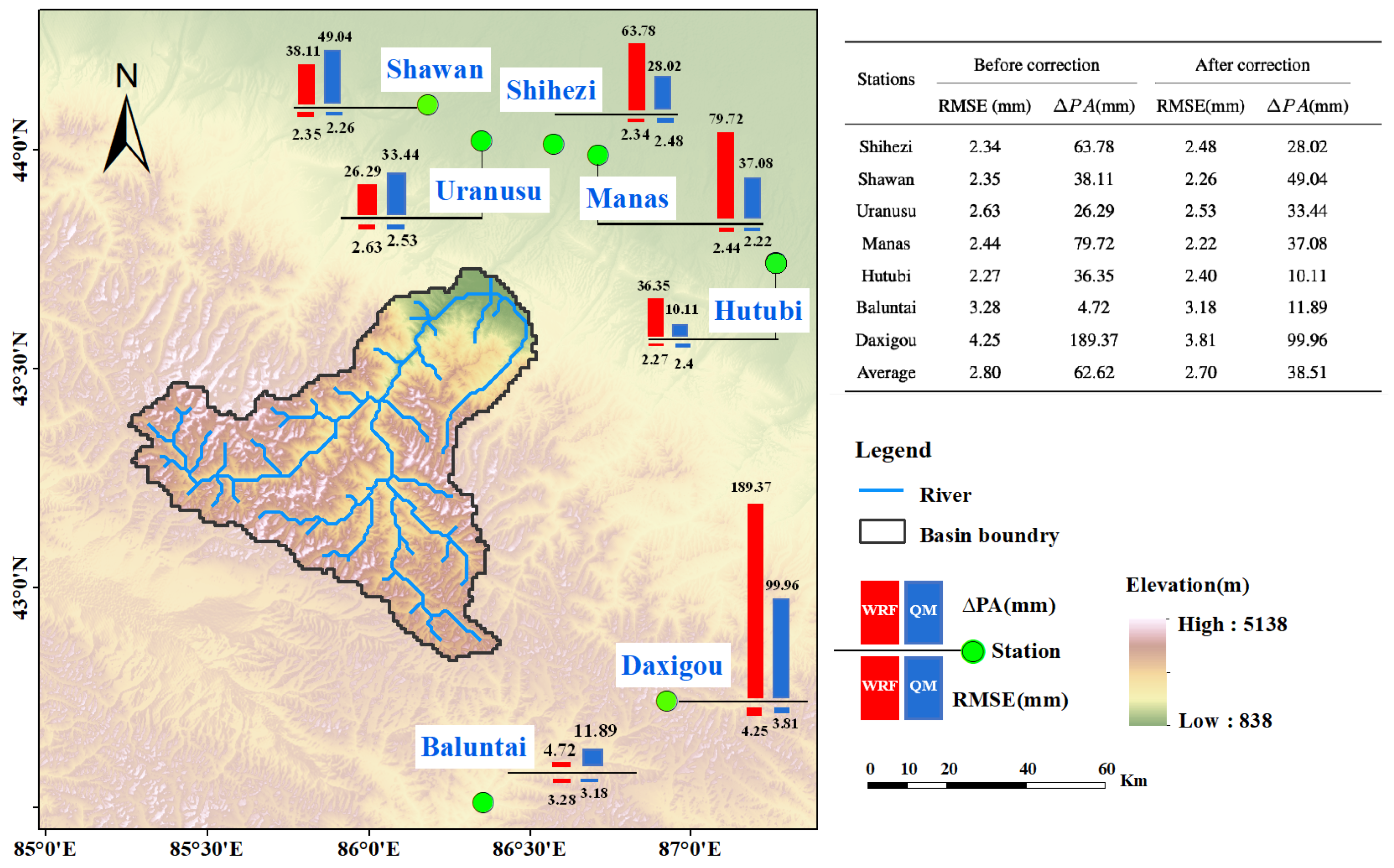
We compared the WRF downscaled precipitation and frequency-corrected precipitation (QM precipitation) with the meteorological station observations to illustrate how precipitation accuracy could be improved by frequency-correcting the WRF precipitation (Figure 3). Since there are no stations in the Manas basin, we compared them with seven stations near the basin. Here, only WRF precipitation and QM precipitation were chosen for validation because the GRIDDED precipitation results from interpolating the station observations.
For the total volume errors (), the QM precipitation performs better on four stations, whereas the of WRF precipitation has significant errors. For example, the in the Daxigou station decreased from 189.37 mm to 99.96 mm and from 79.72 mm to 37.08 mm in the Manas station. In the other three stations with lower in the WRF precipitation, the frequency-corrected QM precipitation has a slightly larger than the WRF precipitation. For example, the increases from 26.29 mm to 33.44 mm in Uranusu station. In general, frequency correction can reduce the total volume of errors, especially large ones.
The QM precipitation performs better on five stations for the Root-Mean-Square Error (). In the other two stations, the RMSE of the QM precipitation is slightly higher than that of the WRF precipitation (2.4 mm vs. 2.27 mm and 2.48 mm vs. 2.34 mm separately). This indicates that frequency correction can reduce the RMSE of precipitation data in most of the stations.
3.1.2. The Differences between the Three Precipitation Datasets at the Basin Scale
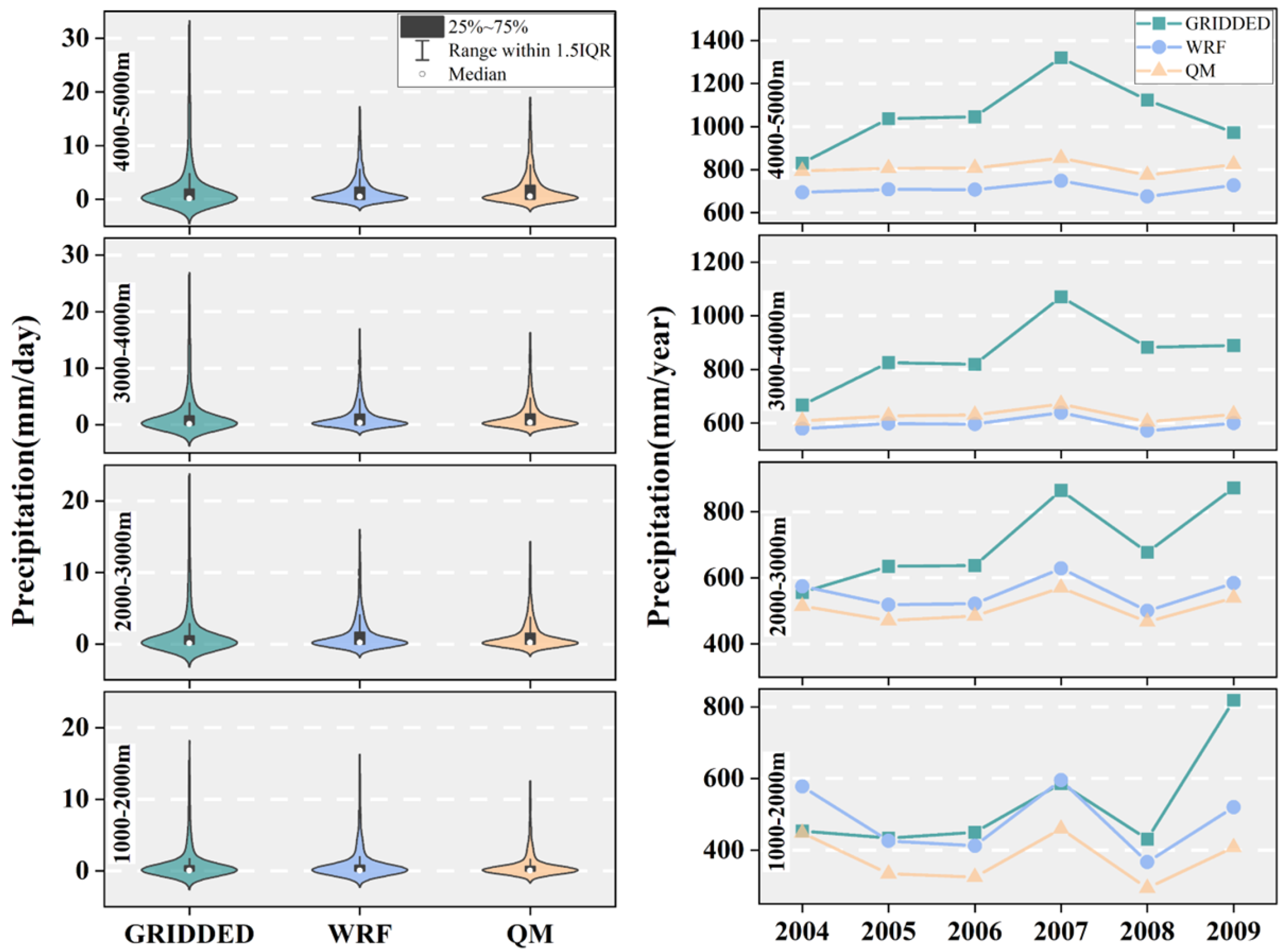
Here, we compared the three precipitation datasets and their hydrological simulation results in four altitude ranges to clarify their differences in hydrological simulation (Figure 4).
The GRIDDED precipitation greatly disagrees with the WRF and the QM precipitation datasets, whether at different altitudes or in annual trends.At all altitudes, the GRIDDED precipitation is greater than the other datasets. For example, in the altitudes from 4000 m to 5000 m, the average annual GRIDDED precipitation is 1054.6 mm, while the others are 709.6 mm and 809.4 mm, separately. The difference is insignificant below 2000 m but enlarged at high altitudes. The annual trend of the GRIDDED precipitation shows a deviation trend from the other datasets, further revealing the clear uncertainty in the GRIDDED data.
The GRIDDED precipitation also exhibits high variations in frequency distribution compared with the other datasets. It has a lower precipitation value concentration but a higher maximum than the other two datasets. This phenomenon is more conspicuous with the increase in altitude. For example, below 2000 m, the median value is 0.04 mm/day. The maximum is 48.8 mm/day for the GRIDDED precipitation, while the median values are 0.07 mm/day and 0.06 mm/day, and the maximums are 65.8 mm/day and 43.2 mm/day for the WRF precipitation and the QM precipitation. However, in altitudes above 4000 m, the median value is 0.14 mm/day, and the maximum is 100.4 mm/day for the GRIDDED precipitation. In contrast, the median values are 0.51 mm/day and 0.57 mm/day, and the maximums are 38.8 mm/day and 38.9 mm/day for the WRF precipitation and the QM precipitation. Although there are no in situ observations above 4000 m in this region, a 100.4 mm/day precipitation event appears impossible. The WRF and QM precipitation are more reliable in the frequency distribution. Therefore, the bias of GRIDDED precipitation data expands with an increase in altitude.
The WRF and QM precipitation are more similar in frequency distribution and annual trend. Above 3000 m, the QM precipitation is greater than the WRF precipitation, while the case is just reversed below an elevation of 3000 m. This means that the frequency correction increased the annual precipitation above 3000 m but did the opposite below 3000 m. The biggest difference between the two datasets can be observed below 2000 m, where the average annual precipitations are 377.8 mm for the QM precipitation and 482.7 mm for the WRF precipitation, respectively. The maximum of the WRF precipitation is 65.9 mm, while it is 43.2 mm for the QM data. This shows that frequency correction mainly works at the lowest altitudes.
3.2. Performance of Frequency-Corrected Precipitation on Simulating the Discharges
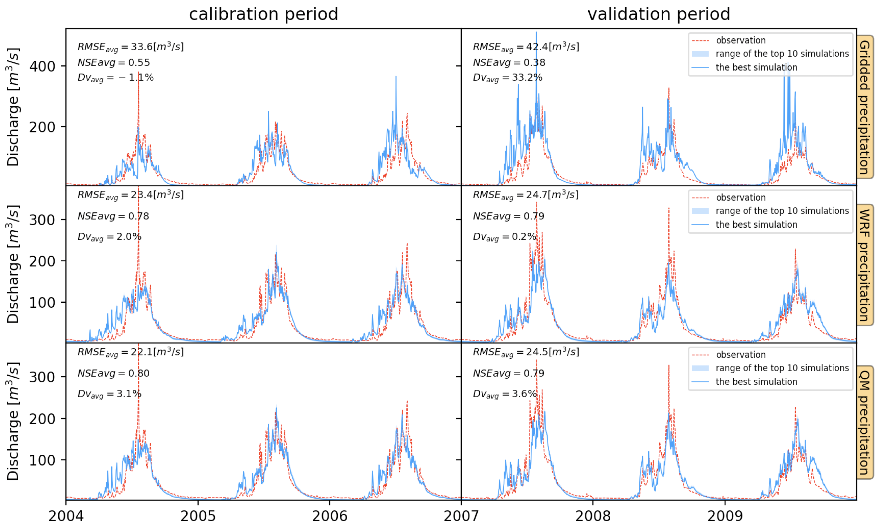
We simulated the daily discharges using the GRIDDED precipitation, the WRF downscaled precipitation, and the QM frequency-corrected precipitation data separately. The SCE-UA algorithm was used to calibrate the GBEHM parameters from 2004 to 2006, then the GBEHM model with calibrated parameters was validated from 2007 to 2009. The ten best simulation results driven by each precipitation data are chosen and shown in Figure 5.
The QM precipitation exhibits the best performance in simulating the discharges. In the calibration period, the QM precipitation-driven results have an average RMSE of 22.1 m3/s, NSE of 0.80, and Dv of 3.1%, while showing an average RMSE of 24.5 m3/s, NSE of 0.79 and Dv of 3.6% in the validation period. The WRF precipitation-driven results demonstrate a comparable accuracy with the QM precipitation. The RMSE of the WRF precipitation-driven discharges is slightly larger than that of the QM, while the NSE and Dv are slightly lower than those of the QM. Regardless of the QM or WRF precipitation, the calibrated model performs similarly throughout calibration and validation periods.
The GRIDDED precipitation-driven results show the worst performance. In the calibration period, the GRIDDED precipitation-driven results have an average RMSE of 33.6 m3/s which is clearly larger than the QM. It has an NSE of 0.55, obviously lower than the QM. In the validation period, all accuracy indicators are significantly worse than in the calibration period, while the average RMSE is 42.4 m3/s, NSE is 0.38, and Dv is 33.2%. Furthermore, this indicates that the GRIDDED precipitation data contain large annual uncertainties and errors because the calibrated model shows no consistent and good performances in the validation period.
We observed that there are still some instances of extreme discharge in three cases, particularly in 2004, 2007, and 2008, which have not been simulated well. This may be because the GRIDDED precipitation product only uses precipitation information from weather stations outside the basin, while the WRF product does not adequately capture these extreme precipitation processes. The frequency-corrected precipitation produced using both sources similarly fails to reflect the extreme precipitation information. This indicates that these extreme precipitation processes are not accurately reflected in any of the three precipitation products. In high-altitude areas, there is a need to increase the temporal resolution of precipitation observations to obtain information on extreme precipitation.
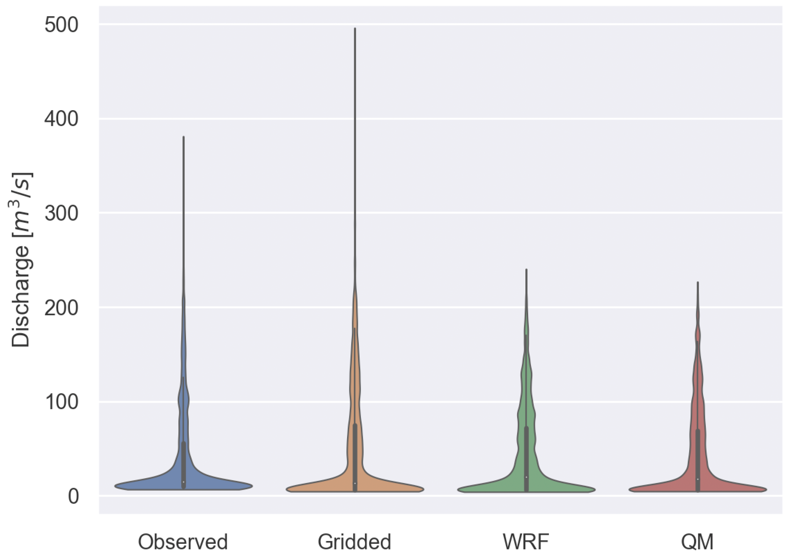
We then compared the three cases’ performances in frequency distribution (Figure 6). The mean value, the concentred range, and the outliers were investigated.
After frequency correction of the WRF data, the mean simulated discharge for the QM precipitation is 42.6 m3/s, similar to the observation of 41.7 m3/s. The mean simulated discharges are 43.8 m3/s for the WRF precipitation case and 48.5 m3/s for the GRIDDED precipitation case. QM precipitation demonstrates the best performance in simulating the mean discharges.
The observed discharges concentrate between 9.5 mm and 55.8 mm (from first to third quartile), the GRIDDED precipitation-driven discharges concentrate between 6.2 mm and 74.7 mm, the WRF precipitation-driven discharges concentrate between 6.1 mm and 71.8 mm, and the QM-precipitation-driven discharges concentrate between 6.0 mm and 69.2 mm. This shows that the QM results are closer to the third quartile than the observation.
In terms of the distribution of the outliers, the mean value of the measured runoff >1.5 IQR outliers of the QM precipitation case is 133.1 mm, which is closest to the observation of 127.8 mm, while it is 137.0 mm and 158.7 mm for the WRF case and the GRIDDED case, respectively. The GRIDDED case has the most considerable discharge bias, especially in peak flow simulation. This also can be observed in Figure 5 where the WRF case is better than the GRIDDED case. After frequency correction of the WRF data, the QM case performance improved slightly from 137.0 mm to 133.1 mm.
In general, the QM precipitation case outperforms the other cases compared to the simulated discharge frequency. Our results indicate that the QM precipitation can be used to optimize the discharge simulation by frequency-correcting the WRF precipitation data.
3.3. Evaluation of Simulated Runoff Depth and Evaporation Driven by Three Precipitation Datasets
3.3.1. Annual Precipitation, Evaporation, Runoff Depth and Runoff Coefficient
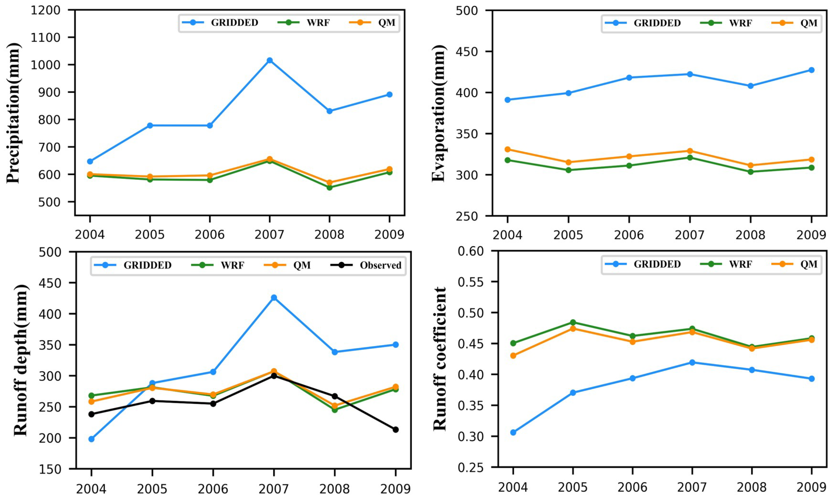
We averaged the annually observed discharges to the Manas basin and obtained a reference annual runoff depth of 255.4 mm (Figure 7). The average annual runoff depth was 274.5 mm for the WRF case, 274.9 mm for the QM case, and 317.4 mm for the GRIDDED case from 2004 to 2009. The simulated runoff depths using the WRF and the QM precipitation data are highly consistent with the reference runoff depth. In contrast, the simulated runoff depth using GRIDDED diverges from the truth. The GRIDDED result also shows a significant variation from the lowest 200 mm to the highest, almost 450 mm, while the WRF and the QM runoff depths remain stable between 240 mm and 310 mm.
The GRIDDED annual precipitation largely ranges between 600 mm and 1100 mm, resulting in a similar fluctuation in runoff depth. Still, the WRF and QM precipitation ranges are steady and limited at approximately 600 mm. The GRIDDED evaporation is relatively stable but has no significant variation like the corresponding precipitation and runoff. As a statistical result, the average annual precipitation in the Manas River basin is 823.3 mm for GRIDDED, 593.8 mm for WRF, and 605.4 mm for the QM from 2004 to 2009. The average annual evaporation is 411.0 mm for the GRIDDED case, 311.3 mm for the WRF case, and 321.2 mm for the QM case.
For the runoff coefficient, the GRIDDED precipitation was also misestimated. The GRIDDED averaged annual runoff coefficient is 0.38, while the WRF is 0.46, and the QM is 0.45. The runoff coefficients of the WRF and QM cases hold a stable value of about 0.45. However, the runoff coefficient of the QM case shows a large change from 0.3 to 0.4, which seems unreasonable considering the cold region basin usually has a stable runoff coefficient.
In general, the GRIDDED-precipitation-driven results deviate significantly from the actual ones, and no reasonable results can be obtained despite the utilization of the parameter calibration. The WRF and the QM results are more consistent with the actual results, and the two show no clear differences in simulating annual runoff and evaporation.
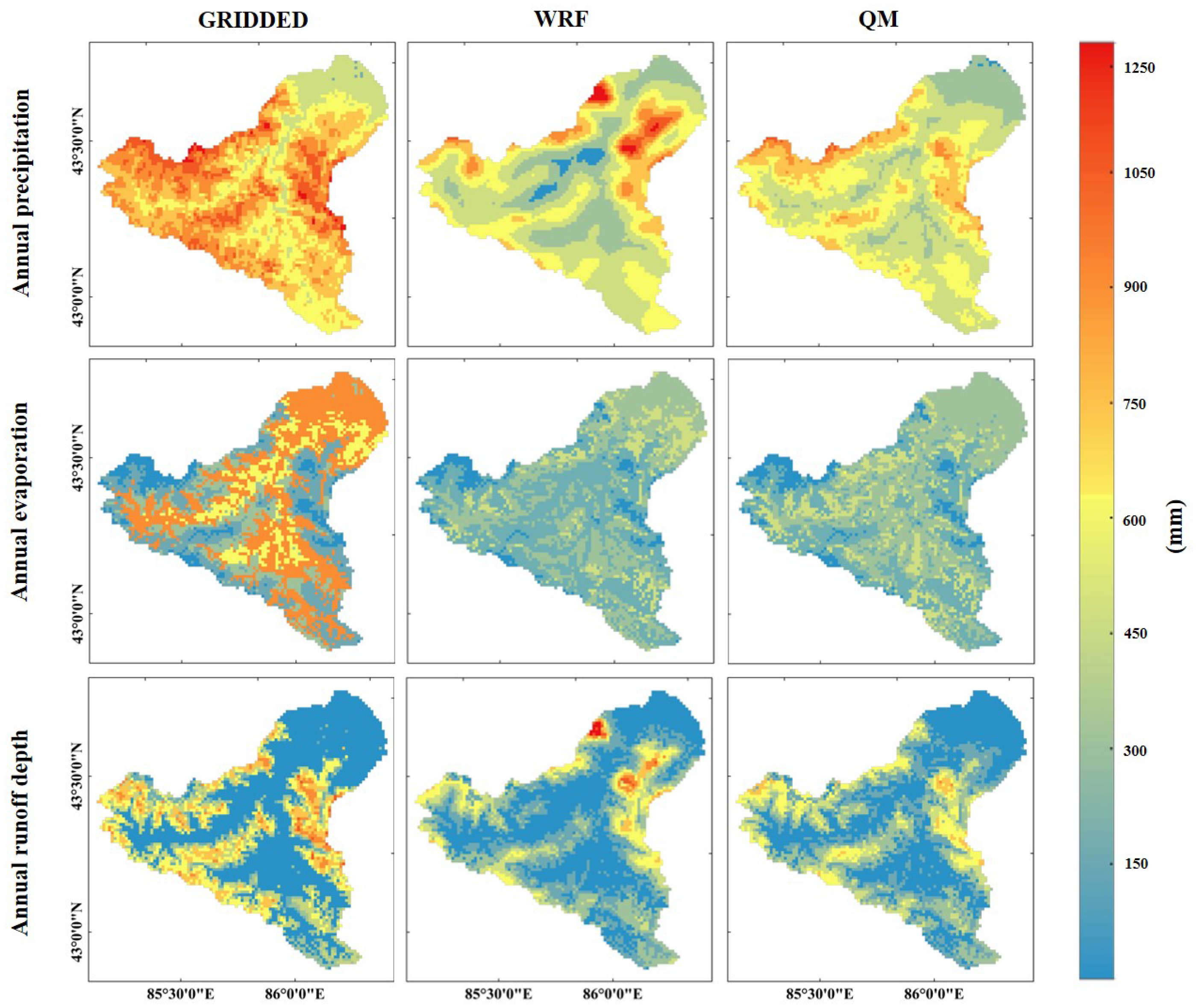
From the spatially distributed precipitation maps (Figure 8), it can be noticed that the GRIDDED precipitation values are significantly greater than the other two datasets and are correlated closely with altitude. The spatial distribution of WRF precipitation exhibits a correlation with, but is not entirely dependent on, altitude; for instance, the values of WRF precipitation are higher in the northern lower mountainous and lower in the southern higher mountainous. This may be because the WRF precipitation is derived from simulations of dynamical processes that consider topographic features and the physical processes of water vapor transportation. The QM precipitation further reduces the spatial differences in the WRF precipitation, and some of the WRF data’s excessive values are corrected.
According to the results of the spatial distribution of simulated evaporation, the evaporation simulated by the GRIDDED precipitation exhibits strong heterogeneity, and the spatial differences in evaporation can reach 600 mm, which is obviously not representative of the actual situation. In contrast, the spatial distribution of evaporation derived from the WRF and QM precipitation is more consistent.
According to the spatially distributed runoff depth, the runoff depths obtained from the GRIDDED precipitation exhibit strong spatial heterogeneity, with high values concentrated in the high elevations and small values in the low-elevation areas. In addition, the runoff depths obtained from the WRF precipitation and the QM precipitation are spatially similar, except that the WRF-driven runoff depths have several high-value areas in the north of the basin, which differs from the QM-driven runoff depths.
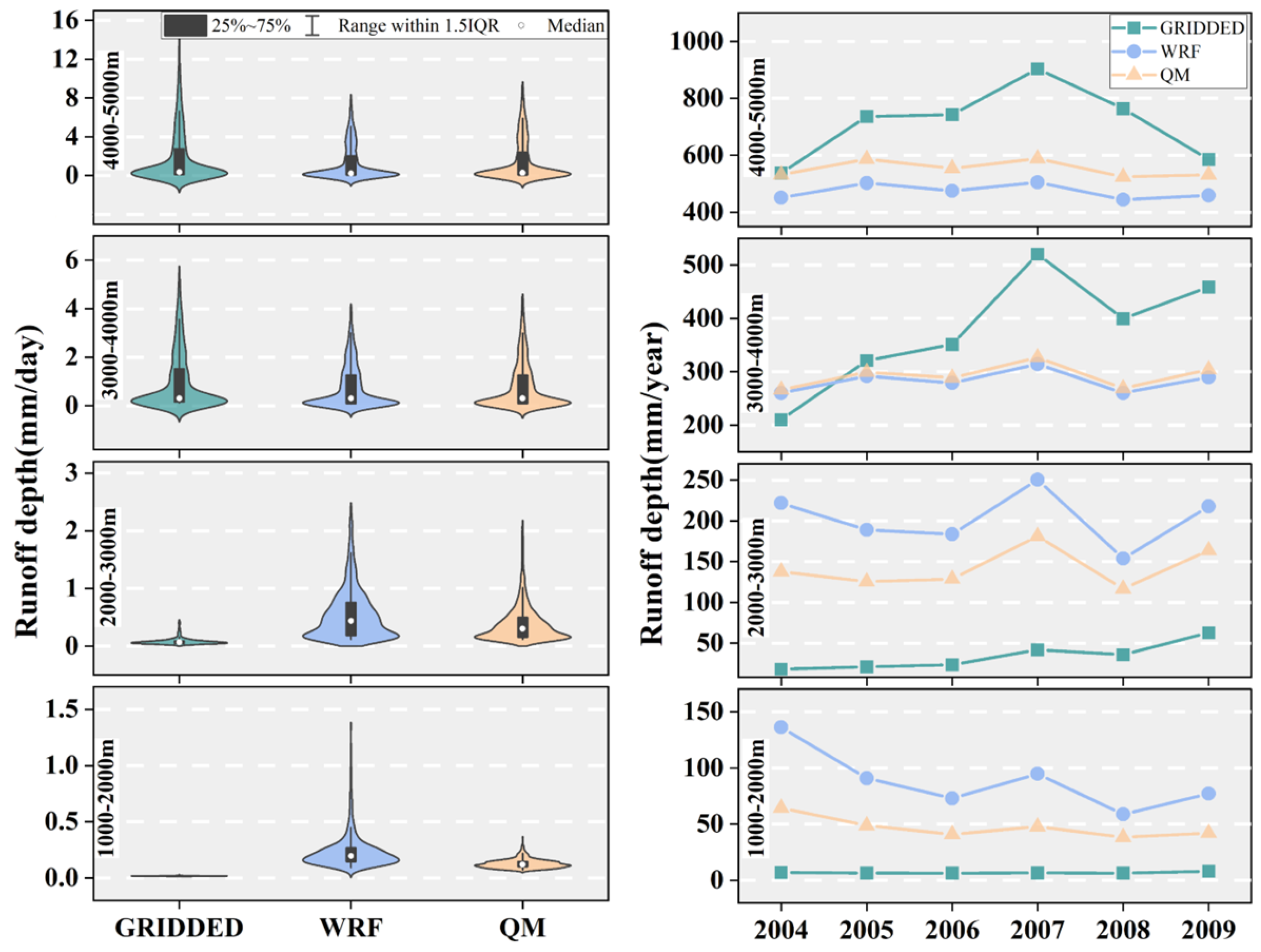
3.3.2. The Altitude Difference of Simulated Runoff Depth Driven by Three Precipitation Datasets
The QM annual runoff depth is between the GRIDDED and WRF cases (Figure 9). Since the WRF precipitation is a correction from the QM precipitation, it can be seen that the QM precipitation increases runoff depth in the regions above 3000 m elevation relative to the WRF precipitation. In contrast, below 3000 m, the QM precipitation decreases runoff depth relative to the WRF precipitation. This suggests that the QM precipitation promotes runoff generation in the region above 3000 m while suppressing runoff generation below 3000 m, consistent with the elevation distribution of the QM and the WRF precipitation in the previous section. Similar results can be seen in the frequency distribution plots (Figure 9). Most notably, in the region below 2000 m elevation, the WRF case has higher values distribution of runoff depth relative to the QM case. At this elevation, the maximum QM runoff depth is 0.6 mm/day, and the median value is 0.1 mm/day, while the maximum WRF runoff depth is 2.0 mm/day, and the median value is 0.2 mm/day. Furthermore, at the 2000–3000 m elevation range, the frequency distribution of runoff depth from the QM precipitation is significantly lower in the moderate and high values than in the WRF case.
The GRIDDED precipitation produces very little runoff depth below 3000 m, especially in the region below 2000 m, where almost no flow is produced. In contrast, the runoff depth is very high, and the frequency distribution is uneven in high-altitude areas above 3000 m. This is closely related to the high heterogeneity of the GRIDDED precipitation over the elevation gradient. Comparatively, the annual variation in runoff depth regarding the WRF and QM cases is smoother and more consistent with the actual situation.
We noticed that the lower-altitudes precipitation values do not vary much for the three precipitation datasets, especially below 2000 m. However, the simulated runoff depths differ greatly between the GRIDDED case and the others in this altitude range. This conflict might have a reasonable explanation if we observe two facts: the conspicuously higher values of the GRIDDED precipitation in other higher altitudes and the global parameter optimization algorithm (SCE-UA) would find the best discharge simulation by adjusting the global parameters. Since the GRIDDED precipitation has unusually high precipitations in higher altitudes, the SCE-UA algorithm would lower the runoff generation of the entire altitudes to meet the actual discharge observation, leading to a distortion of the distributed spatially runoff generation. In this distorted situation for the GRIDDED case, the higher altitudes still have higher runoff generation. In comparison, the lower altitudes have underestimated runoff generation, leading to a good surface look in converged discharge.
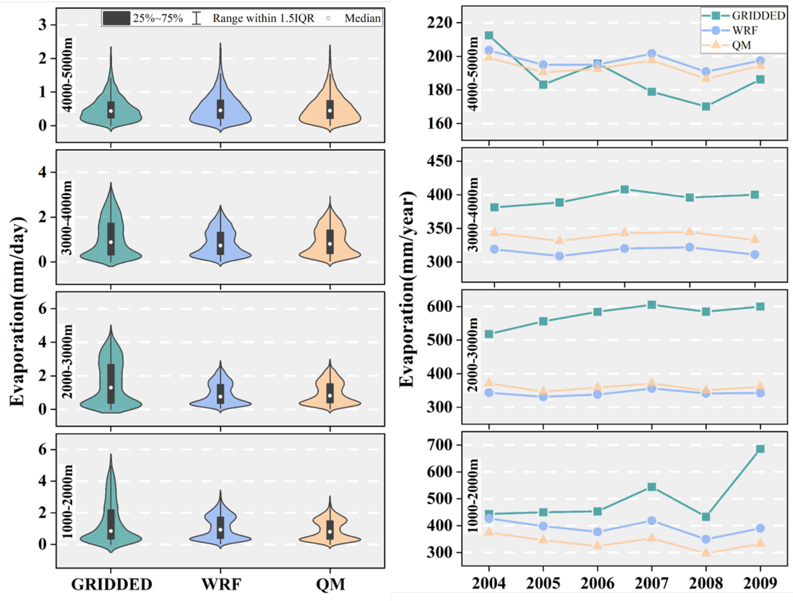
3.3.3. The Altitude Difference of Simulated Evaporation Driven by Three Precipitation Datasets
The frequency distribution of the evaporation corresponding to the three precipitation datasets is more similar above an altitude of 4000 m than at other altitudes (Figure 10). The median values are 0.4 mm/day for the GRIDDED precipitation case, 0.5 mm/day for the WRF precipitation case, and 0.4 mm/day for the QM case. The maximum values are 2.6 mm, 2.6 mm, and 2.5 mm for the three cases. Above the altitude of 4000 m, Figure 9 indicates that the GRIDDED precipitation is significantly greater than the other two precipitation datasets, which indicates that the amount of precipitation does not have a major effect on evaporation and sublimation in cold conditions at high altitudes. Furthermore, as the altitude decreases and the air temperature gradually increases, the evaporation corresponding to the GRIDDED precipitation appears significantly different from the other two cases. In particular, the difference is most pronounced in the 2000–3000 m region. In this altitude range, the average annual evaporation corresponding to the GRIDDED precipitation is 574.4 mm, while it is 342.2 mm for the WRF case and 359.7 mm for the QM case.
The frequency distributions of the evaporation for the QM and WRF cases are relatively close and are most similar at high elevations above 4000 m, while the differences are not significant at other elevations. For example, the difference in the frequency distribution of evaporation between the two at low elevations below 2000 m is also insignificant, in contrast to the distribution of runoff depth at the same elevation (Figure 9). This indicates that the spatial heterogeneity of the evaporation for the WRF and QM cases is weaker than their stronger spatial heterogeneity of runoff depth.
Comparing the annual evaporation for the QM and the WRF cases, the trends of both are very similar. As for the annual evaporation comparison, the QM case’s evaporation is slightly larger than the WRF case in the 2000–4000 m elevations, while the evaporation of the QM case is slightly smaller than the WRF case in the area of 4000 m above and 2000 m below. It differs greatly from the precipitation and runoff depth at different elevations for the QM and WRF cases. This further indicates that, apart from precipitation, meteorological elements such as air temperature play a stronger role in evaporation.
In summary, the interpolation of precipitation using a few stations in ungauged high-altitude areas is generally unreliable and also affects the accuracy of the simulated evaporation and other hydrological elements; using the atmospheric model for dynamic downscaling can obtain a better precipitation distribution and can simulate a relatively reliable discharge process; discharge, runoff depth, and evaporation can be more accurately simulated, with frequency-correcting the atmospheric model (WRF) precipitation.
4. Discussion
Through the numerical experiment, we investigated the performance of frequency-corrected precipitation in ungauged high mountain hydrological simulation and obtained some key findings. Here, we interpret our findings to address our motivations behind this study mentioned in the introduction, and discuss these findings from the perspective of previous studies.
4.1. The Implications of Evaluating the Gridded Precipitation Data on Simulating the Ungauged High Mountain Hydrological Processes
Our study emphasizes that the gridded precipitation bears many uncertainties and is unreliable in hydrological simulation in ungauged high-altitude areas. This is consistent with previous studies, which indicate that the number and spatial coverage of surface stations limit the reliability of precipitation data [16]. In Ref. Gampe and Ludwig [45], the authors also suggested that the higher-resolution gridded precipitation datasets show a better agreement with the overall climatology, and the researchers in Raimonet et al. [46] pointed out that high-resolution meteorological datasets were better at simulating streamflow than coarse-resolution ones. These studies all suggested that fewer station observations would introduce more uncertainties in hydrological simulation.
Extending beyond previous studies, we find that these uncertainties distort the spatial runoff generation if an optimization algorithm is used to calibrate the hydrological simulation. Even by parameter calibration, the model driven by the gridded precipitation has no reliable and consistent discharge simulation in the validation period. We also noticed that the uncertainty relates to the existing stations’ spatial locations or altitudes. In our study, most of the stations used in the interpolation are located in the lower altitudes, leading to a significant bias of gridded precipitation in higher altitudes, which matches our observation that the errors of gridded precipitation data expand with the altitude increase.
These findings suggest that more representative meteorological stations should be used for a reasonable gridded dataset. These stations should at least have an altitude representation if the number of stations is limited in remote ungauged high mountain basins.
4.2. The Advantages of Frequency-Corrected Precipitation in Hydrological Simulation
Our results indicate that frequency correction can effectively reduce the total volume of errors in the WRF precipitation, especially where errors are significant. The quantile-mapping precipitation significantly improves frequency distribution and total volume, although only a few stations can provide precipitation frequency distribution information. Our results are consistent with previous studies, which suggested that the quantile mapping method may improve the precipitation evaluation in most cases. For example, researchers in Reiter et al. [22] found that applying quantile mapping to subsamples can improve the bias correction of daily precipitation, while the authors of Heo et al. [24] found that two-shape parameter distribution models can improve the performance of the quantile mapping method in the bias correction of precipitation data.Previous studies also suggested that the effectiveness of quantile mapping may vary depending on the topographic conditions, parameter sets used, and the transformation function itself [47]. In our case, we noticed that the precipitation data from the QM correction show some improvement but not much. This may be related to the availability of the station observations since there are only seven stations around the study basin.
Numerous studies have evaluated the performance of different precipitation data in hydrological simulations [25,26,48]. However, there is no clear clarification on how the frequency correction could influence the hydrological simulation. In this study, we proved that the frequency distribution should be paid more attention in hydrological simulation aside from the precipitation’s total or mean volume. Although the total volumes of the precipitation datasets are similar, the simulated discharges could show different performances. For example, in our study, the QM and the WRF have similar total volumes but different frequencies at different altitudes, leading to a different simulation of discharges. This partially agrees with the opinion of Qi et al. [49] whereby a better precipitation accuracy on total volume does not guarantee a better discharge simulation.
Our study also indicates that despite the direct interpolated gridded precipitation not being suitable for mountain hydrological simulation, the frequency information from the existing few stations could help correct the WRF precipitation. Furthermore, it suggests that using frequency information but not direct interpolation could be a choice for the ungauged basin.
In this study, we proposed a global parameter optimization method to evaluate the precipitation performance in simulating hydrological processes. Because this method can avoid the influence of the artificial choice of parameters and assess the discharge and evaporation, we suggest that it is a more fair and reliable approach. Some studies have indicated that the hydrological simulated streamflow and evaporation can be used to evaluate precipitation data [27]. The authors of Wang et al. [50] also suggested that the flexibility of hydrological models is mostly determined by adjusting evapotranspiration and soil moisture storage to reduce bias. These studies implied that the simulated evaporation could be used to indirectly assess the performance of precipitation data in hydrological simulation. However, the influence of frequency-corrected precipitation on the simulated evaporation is also not clarified in previous studies.
In our study, we compare the performance of simulated evaporation from the three precipitation datasets. Based on the evaluation of the altitude-related evaporation and precipitation, we find that even with significant bias in precipitation in higher altitudes, the evaporation shows no coordinative difference in simulated evaporation because meteorological elements, such as air temperature, play a stronger role in the evaporation process at cold high altitudes.
4.3. How the Findings Could Be Used in Other Similar Areas
Our study suggests that having more stations at different altitudes is necessary to measure precipitation accurately. Increasing the number of station observations is a straightforward solution to address this issue. With technological advances, building remote area instruments is not as difficult as before. The popular concept of the ’Internet of Things’ could be beneficial in this regard [51]. Some high mountain observation systems are also in construction [52]. However, measuring precipitation requires special instruments, such as carefully maintained precipitation instruments. Therefore, although crucial, not many representative stations could be helpful. Our studies have emphasized the importance of selecting representative stations at different altitudes, which could be a reference in building necessary in situ stations.
Our study suggests a feasible flow for precipitation preparation for ungauged remote high mountain areas. If there are no ground stations, reanalysis of precipitation data is more reliable than gridded data from very remote stations. If a few stations are near the study area, it is suggested that one uses an atmosphere model downscaled precipitation as the base data, and then the frequency information of precipitation from available near stations can be used to correct the base precipitation.
When applying the precipitation preparation flow, the choice of model parameters is a potential factor that could influence the evaluation results. Since we used a physically based hydrological model, the parameter choice seldom affects the model. However, it should be noted that some parameters, such as soil information, remain unchanged, which may introduce uncertainties in the evaluation. When using an empirical model to perform a similar job, the choice of parameters should be paid more attention to ensure a comprehensive global parameter search as much as possible.
In summary, our findings indicate that the frequency-corrected precipitation can effectively improve the hydrological simulation performance, even though only a few stations could provide the available information on the precipitation frequency distribution. This improvement is not only in modeling discharge and runoff depth but also in evaporation. Our study provides a feasible flow for future precipitation preparation for similar ungauged high mountain areas. Frequency correction, instead of direct interpolation, may be a viable option for precipitation preparation. Our research also emphasized the importance of precipitation observation’s altitudinal frequency information, indicating the need to install key representative stations at different altitudes.
5. Conclusions
We assessed the performance of precipitation datasets in hydrological simulations in an ungauged high mountain basin. A global parameter optimization approach was used in this method without artificial parameter selection, making it more fair and reliable.
Our study highlights the significance of precipitation frequency correction in hydrological simulations. Although only a few stations can offer frequency information of precipitation, the frequency-correction approach (quantile mapping) can be utilized to reduce the total volume of errors in the reanalysis precipitation data, particularly where errors are severe. Although the overall volumes of the precipitation datasets before and after the frequency correction are similar, the simulated discharges can demonstrate distinct performances. The frequency-corrected precipitation performs better in modeling discharge and evaporation regarding the total volume and altitude-related characteristics.
Our results suggest that the high uncertainty in the gridded precipitation can be attributed to its unreliable frequency distribution. The gridded precipitation data bear high uncertainties in frequency in the hydrological model simulation, which distorts spatial runoff generation. The station locations and altitude affect the uncertainty because most stations used in the interpolation are at lower altitudes, resulting in a considerable bias of gridded precipitation at higher altitudes. Our study also examined altitude-related evaporation of different precipitation datasets. Even with significant bias in precipitation at higher altitudes, simulated evaporation has no coordinative difference because meteorological elements, such as air temperature, play a stronger role in evaporation at cold high altitudes.
This shows that frequency correction, instead of direct interpolation, may present a viable option for precipitation preparation in similarly ungauged high mountain basins. In the absence of ground stations, reanalysis precipitation data are more reliable than gridded data when only a few stations are within close proximity. The frequency information from the few existing stations could help correct the reanalysis precipitation data. Our study suggests that having more stations at different altitudes is necessary to measure precipitation accurately in similarly ungauged high mountain areas. These stations are crucial and should be representative for a reasonable gridded dataset, especially on the altitude representation for the remotely ungauged high mountain basins.
Author Contributions
Conceptualization, H.L.; methodology, H.L. and J.M.; software, H.L. and J.M.; validation, H.L. and J.M.; writing—original draft preparation, H.L.; writing—review and editing, H.L., J.M., Y.Y. and L.N.; visualization, Y.Y. and L.N.; supervision, H.L.; Data, X.L. All authors have read and agreed to the published version of the manuscript.
Funding
This research was funded by the Basic Research Operating Expenses of the Central Level Non-profit Research Institutes under grant number IDM2020006 and the Fengyun Application Pioneering Project under grant number FY-APP-2022.0401.
Data Availability Statement
The data presented in this study are available on request from the corresponding author. The data are not publicly available due to the data sharing policy.
Conflicts of Interest
The authors declare no conflict of interest.
Abbreviations
The following abbreviations are used in this manuscript:
| 3DTPS | Three-dimensional thin plate spline |
| CFDDA | NCAR Global Climate Four-Dimensional Data Assimilation |
| ECMWF | European Centre for Medium-Range Weather Forecasts |
| ERA | European Re-Analysis |
| Dv | Volume Difference |
| GBEHM | Geomorphology-Based Eco-Hydrological Model |
| GCM | General Circulation Model |
| HAR | High Asia Refined analysis |
| IQR | InterQuartile Range |
| JRA-55 | Japanese 55-year Reanalysis |
| NCEP | National Centers for Environmental Prediction |
| NCEP-CFSR | NCEP Climate Forecast System Reanalysis |
| NSE | Nash–Sutcliffe Efficiency coefficient |
| QM | Quantile Mapping |
| RCM | Regional Climate Model |
| RMSE | Root-Mean-Square Error |
| SCE-UA | Shuffled Complex Evolution |
| WRF | ERAQuantileMappingWeather Research and Forecasting |
References
- Wortmann, M.; Bolch, T.; Menz, C.; Tong, J.; Krysanova, V. Comparison and Correction of High-Mountain Precipitation Data Based on Glacio-Hydrological Modeling in the Tarim River Headwaters (High Asia). J. Hydrometeorol. 2018, 19, 777–801. [Google Scholar] [CrossRef]
- Anders, A.M.; Roe, G.H.; Hallet, B.; Montgomery, D.R.; Finnegan, N.J.; Putkonen, J. Spatial patterns of precipitation and topography in the Himalaya. In Tectonics, Climate, and Landscape Evolution; Willett, S.D., Hovius, N., Brandon, M.T., Fisher, D.M., Eds.; Geological Society of America: Kennewick, WA, USA, 2006; Volume 398, pp. 39–53. [Google Scholar] [CrossRef] [Green Version]
- Li, D.; Yang, K.; Tang, W.; Li, X.; Zhou, X.; Guo, D. Characterizing precipitation in high altitudes of the western Tibetan plateau with a focus on major glacier areas. Int. J. Climatol. 2020, 40, 5114–5127. [Google Scholar] [CrossRef]
- Sun, H.; Su, F.; Yao, T.; He, Z.; Tang, G.; Huang, J.; Zheng, B.; Meng, F.; Ou, T.; Chen, D. General overestimation of ERA5 precipitation in flow simulations for High Mountain Asia basins. Environ. Res. Commun. 2021, 3, 121003. [Google Scholar] [CrossRef]
- Zhang, Y.; Li, J. Impact of moisture divergence on systematic errors in precipitation around the Tibetan Plateau in a general circulation model. Clim. Dyn. 2016, 47, 2923–2934. [Google Scholar] [CrossRef] [Green Version]
- Wang, L.; Zhang, F.; Zhang, H.; Scott, C.A.; Zeng, C.; Shi, X. Intensive precipitation observation greatly improves hydrological modelling of the poorly gauged high mountain Mabengnong catchment in the Tibetan Plateau. J. Hydrol. 2018, 556, 500–509. [Google Scholar] [CrossRef]
- Tang, X.; Zhang, J.; Wang, G.; Ruben, G.B.; Bao, Z.; Liu, Y.; Liu, C.; Jin, J. Error Correction of Multi-Source Weighted-Ensemble Precipitation (MSWEP) over the Lancang-Mekong River Basin. Remote. Sens. 2021, 13, 312. [Google Scholar] [CrossRef]
- Chen, H.; Yong, B.; Gourley, J.J.; Liu, J.; Ren, L.; Wang, W.; Hong, Y.; Zhang, J. Impact of the crucial geographic and climatic factors on the input source errors of GPM-based global satellite precipitation estimates. J. Hydrol. 2019, 575, 1–16. [Google Scholar] [CrossRef]
- Jiang, Q.; Li, W.; Fan, Z.; He, X.; Sun, W.; Chen, S.; Wen, J.; Gao, J.; Wang, J. Evaluation of the ERA5 reanalysis precipitation dataset over Chinese Mainland. J. Hydrol. 2021, 595, 125660. [Google Scholar] [CrossRef]
- Harada, Y.; Kamahori, H.; Kobayashi, C.; Endo, H.; Kobayashi, S.; Ota, Y.; Onoda, H.; Onogi, K.; Miyaoka, K.; Takahashi, K. The JRA-55 Reanalysis: Representation of Atmospheric Circulation and Climate Variability. J. Meteorol. Soc. Japan. Ser. II 2016, 94, 269–302. [Google Scholar] [CrossRef] [Green Version]
- Ihsan, H.M.; Nurrohman, A.W.; Sahid. Assessment of NCEP-CFSR Precipitation Products in Meteorological Drought Monitoring for The Citarum Basin. IOP Conf. Ser. Earth Environ. Sci. 2019, 286, 012019. [Google Scholar] [CrossRef]
- Rife, D.L.; Pinto, J.O.; Monaghan, A.J.; Davis, C.A.; Hannan, J.R. NCAR Global Climate Four-Dimensional Data Assimilation (CFDDA) Hourly 40 km Reanalysis. 2014. Artwork Size: 26.975 TB Medium: NetCDF4 Pages: 26.975 TB Type: Dataset. Available online: https://rda.ucar.edu/datasets/ds604.0/ (accessed on 12 December 2022).
- Precipitation Seasonality and Variability over the Tibetan Plateau as Resolved by the High Asia Reanalysis. J. Clim. 2014, 27, 1910–1927. [CrossRef] [Green Version]
- Lundquist, J.; Hughes, M.; Gutmann, E.; Kapnick, S. Our Skill in Modeling Mountain Rain and Snow is Bypassing the Skill of Our Observational Networks. Bull. Am. Meteorol. Soc. 2019, 100, 2473–2490. [Google Scholar] [CrossRef] [Green Version]
- Hu, Z.; Hu, Q.; Zhang, C.; Chen, X.; Li, Q. Evaluation of reanalysis, spatially interpolated and satellite remotely sensed precipitation data sets in central Asia. J. Geophys. Res. Atmos. 2016, 121, 5648–5663. [Google Scholar] [CrossRef] [Green Version]
- Sun, Q.; Miao, C.; Duan, Q.; Ashouri, H.; Sorooshian, S.; Hsu, K.L. A Review of Global Precipitation Data Sets: Data Sources, Estimation, and Intercomparisons. Rev. Geophys. 2018, 56, 79–107. [Google Scholar] [CrossRef] [Green Version]
- Hay, L.E.; Wilby, R.L.; Leavesley, G.H. A Comparison of Delta Change and Downscaled Gcm Scenarios for Three Mountainous Basins in the United States. J. Am. Water Resour. Assoc. 2000, 36, 387–397. [Google Scholar] [CrossRef]
- Mahmood, R.; Jia, S.; Tripathi, N.K.; Shrestha, S. Precipitation Extended Linear Scaling Method for Correcting GCM Precipitation and Its Evaluation and Implication in the Transboundary Jhelum River Basin. Atmosphere 2018, 9, 160. [Google Scholar] [CrossRef] [Green Version]
- Graham, L.P.; Hagemann, S.; Jaun, S.; Beniston, M. On interpreting hydrological change from regional climate models. Clim. Chang. 2007, 81, 97–122. [Google Scholar] [CrossRef]
- Zhu, Y.; Luo, Y. Precipitation Calibration Based on the Frequency-Matching Method. Weather. Forecast. 2015, 30, 1109–1124. [Google Scholar] [CrossRef]
- Cannon, A.J.; Sobie, S.R.; Murdock, T.Q. Bias Correction of GCM Precipitation by Quantile Mapping: How Well Do Methods Preserve Changes in Quantiles and Extremes? J. Clim. 2015, 28, 6938–6959. [Google Scholar] [CrossRef]
- Reiter, P.; Gutjahr, O.; Schefczyk, L.; Heinemann, G.; Casper, M. Does applying quantile mapping to subsamples improve the bias correction of daily precipitation? Int. J. Climatol. 2018, 38, 1623–1633. [Google Scholar] [CrossRef]
- Zhang, Q.; Gan, Y.; Zhang, L.; She, D.; Wang, G.; Wang, S. Piecewise-quantile mapping improves bias correction of global climate model daily precipitation towards preserving quantiles and extremes. Int. J. Climatol. 2022, 42, 7968–7986. [Google Scholar] [CrossRef]
- Heo, J.H.; Ahn, H.; Shin, J.Y.; Kjeldsen, T.R.; Jeong, C. Probability Distributions for a Quantile Mapping Technique for a Bias Correction of Precipitation Data: A Case Study to Precipitation Data Under Climate Change. Water 2019, 11, 1475. [Google Scholar] [CrossRef] [Green Version]
- Bitew, M.M.; Gebremichael, M. Evaluation of satellite rainfall products through hydrologic simulation in a fully distributed hydrologic model. Water Resour. Res. 2011, 47, 6. [Google Scholar] [CrossRef]
- Ougahi, J.H.; Mahmood, S.A. Evaluation of satellite-based and reanalysis precipitation datasets by hydrologic simulation in the Chenab river basin. J. Water Clim. Chang. 2022, 13, 1563–1582. [Google Scholar] [CrossRef]
- Ghatak, D.; Zaitchik, B.; Kumar, S.; Matin, M.A.; Bajracharya, B.; Hain, C.; Anderson, M. Influence of Precipitation Forcing Uncertainty on Hydrological Simulations with the NASA South Asia Land Data Assimilation System. Hydrology 2018, 5, 57. [Google Scholar] [CrossRef] [Green Version]
- HongBo LING, H.X. Surface runoff processes and sustainable utilization of water resources in Manas River Basin, Xinjiang, China. J. Arid. Land 2012, 4, 271–280. [Google Scholar] [CrossRef] [Green Version]
- Ma, J.; Li, H.; Wang, J.; Hao, X.; Shao, D.; Lei, H. Reducing the statistical distribution error in gridded precipitation data for the Tibetan Plateau. J. Hydrometeorol. 2020, 21, 2641–2654. [Google Scholar] [CrossRef]
- Piani, C.; Haerter, J.O.; Coppola, E. Statistical bias correction for daily precipitation in regional climate models over Europe. Theor. Appl. Climatol. 2010, 99, 187–192. [Google Scholar] [CrossRef] [Green Version]
- Maraun, D.; Widmann, M. Statistical Downscaling and Bias Correction for Climate Research; Cambridge University Press: Cambridge, UK, 2018. [Google Scholar] [CrossRef] [Green Version]
- Yang, D.; Gao, B.; Jiao, Y.; Lei, H.; Zhang, Y.; Yang, H.; Cong, Z. A distributed scheme developed for eco-hydrological modeling in the upper Heihe River. Sci. China Earth Sci. 2015, 58, 36–45. [Google Scholar] [CrossRef]
- Gao, B.; Yang, D.; Qin, Y.; Wang, Y.; Li, H.; Zhang, Y.; Zhang, T. Change in frozen soils and its effect on regional hydrology, upper Heihe basin, northeastern Qinghai–Tibetan Plateau. Cryosphere 2018, 12, 657–673. [Google Scholar] [CrossRef] [Green Version]
- Li, H.; Li, X.; Yang, D.; Wang, J.; Gao, B.; Pan, X.; Zhang, Y.; Hao, X. Tracing Snowmelt Paths in an Integrated Hydrological Model for Understanding Seasonal Snowmelt Contribution at Basin Scale. J. Geophys. Res. Atmos. 2019, 124, 8874–8895. [Google Scholar] [CrossRef]
- Wang, X.; Gao, B. Frozen soil change and its impact on hydrological processes in the Qinghai Lake Basin, the Qinghai-Tibetan Plateau, China. J. Hydrol. Reg. Stud. 2022, 39, 100993. [Google Scholar] [CrossRef]
- Qin, Y.; Yang, D.; Gao, B.; Wang, T.; Chen, J.; Chen, Y.; Wang, Y.; Zheng, G. Impacts of climate warming on the frozen ground and eco-hydrology in the Yellow River source region, China. Sci. Total. Environ. 2017, 605–606, 830–841. [Google Scholar] [CrossRef] [Green Version]
- Shangguan, W.; Dai, Y.; Liu, B.; Zhu, A.; Duan, Q.; Wu, L.; Ji, D.; Ye, A.; Yuan, H.; Zhang, Q.; et al. A China data set of soil properties for land surface modeling. J. Adv. Model. Earth Syst. 2013, 5, 212–224. [Google Scholar] [CrossRef]
- Dai, Y.; Shangguan, W.; Duan, Q.; Liu, B.; Fu, S.; Niu, G. Development of a China Dataset of Soil Hydraulic Parameters Using Pedotransfer Functions for Land Surface Modeling. J. Hydrometeorol. 2013, 14, 869–887. [Google Scholar] [CrossRef] [Green Version]
- Ran, Y.; Li, X.; Lu, L. Evaluation of four remote sensing based land cover products over China. Int. J. Remote. Sens. 2010, 31, 391–401. [Google Scholar] [CrossRef]
- Duan, Q.; Sorooshian, S.; Gupta, V.K. Optimal use of the SCE-UA global optimization method for calibrating watershed models. J. Hydrol. 1994, 158, 265–284. [Google Scholar] [CrossRef]
- Rahnamay Naeini, M.; Analui, B.; Gupta, H.V.; Duan, Q.; Sorooshian, S. Three decades of the Shuffled Complex Evolution (SCE-UA) optimization algorithm: Review and applications. Sci. Iran. 2019, 26, 2015–2031. [Google Scholar] [CrossRef]
- Mirjalili, S. SCA: A Sine Cosine Algorithm for solving optimization problems. Knowl.-Based Syst. 2016, 96, 120–133. [Google Scholar] [CrossRef]
- Houska, T.; Kraft, P.; Chamorro-Chavez, A.; Breuer, L. SPOTting Model Parameters Using a Ready-Made Python Package. PLoS ONE 2015, 10, e0145180. [Google Scholar] [CrossRef] [Green Version]
- Kan, G.; He, X.; Ding, L.; Li, J.; Liang, K.; Hong, Y. A heterogeneous computing accelerated SCE-UA global optimization method using OpenMP, OpenCL, CUDA, and OpenACC. Water Sci. Technol. 2017, 76, 1640–1651. [Google Scholar] [CrossRef] [PubMed] [Green Version]
- Gampe, D.; Ludwig, R. Evaluation of Gridded Precipitation Data Products for Hydrological Applications in Complex Topography. Hydrology 2017, 4, 53. [Google Scholar] [CrossRef] [Green Version]
- Raimonet, M.; Oudin, L.; Thieu, V.; Silvestre, M.; Vautard, R.; Rabouille, C.; Moigne, P.L. Evaluation of Gridded Meteorological Datasets for Hydrological Modeling. J. Hydrometeorol. 2017, 18, 3027–3041. [Google Scholar] [CrossRef]
- Enayati, M.; Bozorg-Haddad, O.; Bazrafshan, J.; Hejabi, S.; Chu, X. Bias correction capabilities of quantile mapping methods for rainfall and temperature variables. J. Water Clim. Chang. 2020, 12, 401–419. [Google Scholar] [CrossRef]
- Mao, R.; Wang, L.; Zhou, J.; Li, X.; Qi, J.; Zhang, X. Evaluation of Various Precipitation Products Using Ground-Based Discharge Observation at the Nujiang River Basin, China. Water 2019, 11, 2308. [Google Scholar] [CrossRef] [Green Version]
- Qi, W.; Zhang, C.; Fu, G.; Sweetapple, C.; Zhou, H. Evaluation of global fine-resolution precipitation products and their uncertainty quantification in ensemble discharge simulations. Hydrol. Earth Syst. Sci. 2016, 20, 903–920. [Google Scholar] [CrossRef] [Green Version]
- Wang, J.; Zhuo, L.; Han, D.; Liu, Y.; Rico-Ramirez, M.A. Hydrological Model Adaptability to Rainfall Inputs of Varied Quality. Water Resour. Res. 2023, 59, e2022WR032484. [Google Scholar] [CrossRef]
- Li, X.; Zhao, N.; Jin, R.; Liu, S.; Sun, X.; Wen, X.; Wu, D.; Zhou, Y.; Guo, J.; Chen, S.; et al. Internet of Things to network smart devices for ecosystem monitoring. Sci. Bull. 2019, 64, 1234–1245. [Google Scholar] [CrossRef] [Green Version]
- Che, T.; Li, X.; Liu, S.; Li, H.; Xu, Z.; Tan, J.; Zhang, Y.; Ren, Z.; Xiao, L.; Deng, J.; et al. Integrated hydrometeorological, snow and frozen-ground observations in the alpine region of the Heihe River Basin, China. Earth Syst. Sci. Data 2019, 11, 1483–1499. [Google Scholar] [CrossRef] [Green Version]
Figure 1.
Flowchart of the experiments. Three precipitation datasets (the GRIDDED, WRF, and QM) were made for comparison. The QM precipitation is from the frequency-corrected WRF precipitation. The GBEHM hydrological model was used to evaluate the precipitation datasets. The SCE-UA optimization method was utilized to calibrate the hydrological model parameters for the three precipitation datasets. The hydrological simulation results driven by the three precipitation datasets were evaluated in four aspects.

Figure 2.
Map of the Manas river basin. The WRF downscaling domain and the hydrological model (GBEHM) simulation domain are illustrated by different rectangles. A schematic representation of the three nesting levels can be seen in the upper left section of the WRF model (d01, d02, d03). The red dashed line shows the operational area of the WRF model domain 3, a 57 × 54 grid with a horizontal resolution of 3.3 km. The yellow dashed line (GBEHM domain) indicates the operational area of the hydrological model, a 111 × 107 grid with a resolution of 1 km. The seven meteorological sites are distributed around the Manas River basin (green triangles). The hydrological outlet gauge (Kenswatt station) is marked with a red circle.

Figure 3.
The accuracy ( and RMSE) of the WRF and QM precipitation datasets are illustrated in the Manas river basin map. The RMSE and are marked as bar charts in which red color represents the accuracy of the WRF precipitation and the blue represents the QM precipitation.
Figure 3.
The accuracy ( and RMSE) of the WRF and QM precipitation datasets are illustrated in the Manas river basin map. The RMSE and are marked as bar charts in which red color represents the accuracy of the WRF precipitation and the blue represents the QM precipitation.

Figure 4.
The left is the altitude-related frequency distribution of precipitation datasets (the GRIDDED precipitation, the WRF downscaled precipitation, and the QM frequency-corrected precipitation data), and the right is the corresponding annual precipitation trend at different altitudes. The IQR used in the legend of the precipitation frequency map denotes interquartile range.

Figure 5.
The simulated discharges using three precipitation datasets (the GRIDDED precipitation, the WRF downscaled precipitation, and the QM frequency-corrected precipitation data). The ten best simulation results calibrated by the SCE-UA algorithm for each precipitation dataset are shown in a blue range. The range is relatively narrow because the ten best simulation results are very close. The simulation period is divided into the calibration period and the validation period. The accuracy indicators (NSE, RMSE, and Dv) of the ten best simulation results were averaged to show the performance of different precipitation datasets. The dashed red line represents the observed discharges.

Figure 6.
A comparison of the frequency distributions between the simulated discharges using different precipitation datasets (the GRIDDED precipitation, the WRF downscaled precipitation, and the QM frequency corrected precipitation data) and the observed discharges.
Figure 6.
A comparison of the frequency distributions between the simulated discharges using different precipitation datasets (the GRIDDED precipitation, the WRF downscaled precipitation, and the QM frequency corrected precipitation data) and the observed discharges.

Figure 7.
A comparison of annual precipitation, evaporation, runoff depth, and the corresponding runoff coefficient from the simulated results of the GRIDDED precipitation, the WRF downscaled precipitation, and the QM frequency corrected precipitation data. The observed runoff depth means the reference annual runoff depth obtained by averaged annual discharges to the whole Manas basin.

Figure 8.
Spatial distribution of annual precipitation, evaporation, and runoff depth from the simulated results by the GRIDDED precipitation, the WRF downscaled precipitation, and the QM frequency corrected precipitation data.
Figure 8.
Spatial distribution of annual precipitation, evaporation, and runoff depth from the simulated results by the GRIDDED precipitation, the WRF downscaled precipitation, and the QM frequency corrected precipitation data.

Figure 9.
The left displays the altitude-related frequency distribution of simulated runoff depth using different datasets (the GRIDDED precipitation, the WRF downscaled precipitation, and the QM frequency-corrected precipitation data), and the right shows the corresponding annual runoff depth trend at different altitudes. The IQR used in the legend of the runoff depth frequency map denotes the interquartile range.

Figure 10.
The left displays the altitude-related frequency distribution of simulated evaporation using different datasets (the GRIDDED precipitation, the WRF downscaled precipitation, and the QM frequency-corrected precipitation data), and the right shows the corresponding annual evaporation trend at different altitudes. The IQR used in the legend of the evaporation frequency map denotes interquartile range.


Table 1.
Key parameters used in the GBEHM model. The soil hydraulic parameters and the soil thermal parameters are from published datasets. The other six parameters to be calibrated are basin uniform.
Table 1.
Key parameters used in the GBEHM model. The soil hydraulic parameters and the soil thermal parameters are from published datasets. The other six parameters to be calibrated are basin uniform.
| Type | Parameter Description | References or Methods |
|---|---|---|
| Parameters to be calibrated | Snow surface roughness | Calibration using SCE-UA |
| Critical temperature for determining rain or snow | Calibration using SCE-UA | |
| Adjustable evaporation resistance | Calibration using SCE-UA | |
| Hydraulic conductivity decay factor | Calibration using SCE-UA | |
| Hydraulic conductivity of ground water | Calibration using SCE-UA | |
| Porosity of Aquifer | Calibration using SCE-UA | |
| Fixed parameters | Soil hydraulic parameters | [37] |
| Soil thermal parameters | [38] | |
| Land cover | [39] |
Disclaimer/Publisher’s Note: The statements, opinions and data contained in all publications are solely those of the individual author(s) and contributor(s) and not of MDPI and/or the editor(s). MDPI and/or the editor(s) disclaim responsibility for any injury to people or property resulting from any ideas, methods, instructions or products referred to in the content. |
© 2023 by the authors. Licensee MDPI, Basel, Switzerland. This article is an open access article distributed under the terms and conditions of the Creative Commons Attribution (CC BY) license (https://creativecommons.org/licenses/by/4.0/).
Share and Cite
MDPI and ACS Style
Li, H.; Ma, J.; Yang, Y.; Niu, L.; Lu, X. Performance of Frequency-Corrected Precipitation in Ungauged High Mountain Hydrological Simulation. Water 2023, 15, 1461. https://doi.org/10.3390/w15081461
AMA Style
Li H, Ma J, Yang Y, Niu L, Lu X. Performance of Frequency-Corrected Precipitation in Ungauged High Mountain Hydrological Simulation. Water. 2023; 15(8):1461. https://doi.org/10.3390/w15081461
Chicago/Turabian StyleLi, Hongyi, Jiapei Ma, Yaru Yang, Liting Niu, and Xinyu Lu. 2023. "Performance of Frequency-Corrected Precipitation in Ungauged High Mountain Hydrological Simulation" Water 15, no. 8: 1461. https://doi.org/10.3390/w15081461
Note that from the first issue of 2016, this journal uses article numbers instead of page numbers. See further details here.