

Research on the Application of CEEMD-LSTM-LSSVM Coupled Model in Regional Precipitation Prediction

Water Conservancy College, North China University of Water Resources and Electric Power, Zhengzhou 450046, China
*
Author to whom correspondence should be addressed.
Water 2023, 15(8), 1465; https://doi.org/10.3390/w15081465
Submission received: 31 January 2023
/
Revised: 6 April 2023
/
Accepted: 7 April 2023
/
Published: 9 April 2023
(This article belongs to the Special Issue Hydroclimatic Modeling and Monitoring under Climate Change)
Abstract
:Precipitation is a vital component of the regional water resource circulation system. Accurate and efficient precipitation prediction is especially important in the context of global warming, as it can help explore the regional precipitation pattern and promote comprehensive water resource utilization. However, due to the influence of many factors, the precipitation process exhibits significant stochasticity, uncertainty, and nonlinearity despite having some regularity. In this article, monthly precipitation in Zhoukou City is predicted using a complementary ensemble empirical modal decomposition (CEEMD) method combined with a long short-term memory neural network (LSTM) model and a least squares support vector machine (LSSVM) model. The results demonstrate that the CEEMD-LSTM-LSSVM model exhibits a root mean square error of 15.01 and a mean absolute error of 11.31 in predicting monthly precipitation in Zhoukou City. The model effectively overcomes the problems of modal confounding present in empirical modal decomposition (EMD), the existence of reconstruction errors in ensemble empirical modal decomposition (EEMD), and the lack of accuracy of a single LSTM model in predicting modal components with different frequencies obtained by EEMD decomposition. The model provides an effective approach for predicting future precipitation in the Zhoukou area and predicts monthly precipitation in the study area from 2023 to 2025. The study provides a reference for relevant departments to take effective measures against natural disasters and rationally plan urban water resources.
1. Introduction
Normal precipitation can contribute to the regional water cycle as a positive feedback process. However, global warming due to greenhouse gas emissions is profoundly affecting regional precipitation patterns, with the IPCC Assessment Report 6 indicating that anthropogenic warming reached about 1 °C (±0.2 °C) in 2017, and that average precipitation in the high northern hemisphere will increase significantly when global warming is 1.5 °C or 2 °C compared to pre-industrial conditions [1]. For example, Chen, J.L. et al. [2] showed that water vapor transport from the Indian monsoon region and the South China Sea in the context of global change becomes an important condition for strong summer precipitation in southern and eastern China; Zhou, T.J. et al. [3] also demonstrated that the alteration of water vapor transport channels in the western Pacific Ocean in the context of global change has a more significant effect on summer precipitation anomalies in China. The increase in precipitation events will inevitably lead to a series of serious consequences, so it is necessary to make accurate predictions of future rainfall trends based on available rainfall data to provide technical support for the sustainable use of regional water resources and disaster prevention and mitigation [4].
Meteorological processes are variable, stochastic, and complex, making precipitation sequences also significantly stochastic, uncertain, and nonlinear [5], increasing the degree of difficulty in accurately predicting precipitation. In recent years, many scholars have conducted extensive research in precipitation prediction, and the methods they use can be broadly classified into two categories: process-based methods and data-driven methods [6]. The purpose of process-based precipitation prediction is to explore the physical processes of precipitation and to identify the various factors that influence the precipitation process. However, the interaction laws among the factors in the precipitation process are very complex, and it is often very difficult to solve and build physical models. The data-driven approach refers to the construction of models based on historical precipitation samples or real-time observation data, and the use of models to dig information, avoiding the analysis of the physical process of precipitation.
The data-driven models that have been widely used include the autoregressive sliding average model, gray model, neural network model, support vector machine model, and random forest. These models have achieved good results in solving complex nonlinearities of precipitation series. For example, Narayana et al. [7] applied the AIRMA model to predict monsoon rainfall in India and concluded that there is an increasing trend of monsoon rainfall; Zhao, Y. [8] used a gray metabolic prediction model to predict future rainfall, which improved the accuracy and precision of traditional gray model prediction results; Gou, Z.J. et al. [9] used a BP neural network to establish a genetic neural network, in which the prediction accuracy of the neural network algorithm for precipitation levels was optimized; Shen, H.J. et al. [10] used a long short-term memory neural network to predict summer precipitation in China in 2014 and 2015, and explored the influence of the starting month data on the seasonal prediction of precipitation. Wang, R. [11] used GIS data as predictors to construct a support vector machine model based on the spatial distribution model of annual rainfall in Handan city, and derived the characteristics of circular aggregation distribution of rainfall in Handan city and the distribution of high and low values of rainfall in the urban area; Sha, S.K. [12] fully combined the unique advantages of the random forest algorithm and established a rainfall prediction model based on the random forest algorithm for the Chengai irrigation area, which improved the accuracy and generalization of the rainfall prediction model.
In the classification of neural network models, the recurrent neural network (RNN) can use state variables to store historical information and be combined with current inputs to jointly determine the output compared to other neural networks [13]. Therefore, it can identify long-term dependencies between precipitation data more effectively, but for long sequences, RNNs suffer from gradient disappearance and excessive gradients during training. Long short-term memory (LSTM) [14] is a special kind of RNN that controls the information transfer by adding unit states and gate structures, solving the gradient disappearance and gradient explosion problems during the training process of long sequences. However, there is still room for optimization of LSTM for precipitation prediction. Wang, W.C. et al. [15] used wavelet decomposition and the coyote optimization algorithm to optimize the accuracy of LSTM model prediction. However, it is difficult for a single LSTM model to accurately predict the actual occurrence of extreme precipitation data in some months, so data denoising methods can be incorporated to improve the prediction accuracy [16].
Empirical modal decomposition (EMD) [17] is one of the most used data denoising methods, and can decompose complex time series data into several intrinsic modal functions (IMFs) and a residual term R, to achieve the exploitation of the frequency domain features of time series. Compared with the original time series data, the analysis and prediction of IMFs and residuals are simpler. However, EMD suffers from modal confounding [18], and the ensemble empirical modal decomposition (EEMD) [19] mitigates the degree of modal confounding in EMD by adding Gaussian white noise to the original sequence and then summing and averaging. Complementary ensemble empirical modal decomposition (CEEMD) [20] adds a pair of positive and negative white noises with opposite numbers to the original time series as auxiliary noise to eliminate the residual white noise in the reconstructed signal after the decomposition of the original EEMD method, and to reduce the number of iterations required for the decomposition and the computational cost.
When decomposing precipitation series using EMD-like methods, the resulting subseries can contain both high-frequency and low-frequency components. To address this issue, the present study proposes a method of dividing the subseries obtained from the EMD-like decomposition into high-frequency and low-frequency subseries for use in building precipitation prediction models. This approach compensates for the limitations of a single algorithm in dealing with different frequency subseries and enables the classification of subseries to facilitate the construction of prediction models.
This paper proposes a method for partitioning high- and low-frequency components in each series obtained from the complete ensemble empirical mode decomposition (CEEMD). The high-frequency subseries are then utilized to construct a prediction model based on the long short-term memory (LSTM) algorithm, whereas the low-frequency sub-series are employed to build a prediction model using the least squares support vector machine (LSSVM) algorithm. The resultant coupled CEEMD-LSTM-LSSVM precipitation prediction model is evaluated using historical precipitation data from Zhoukou city, and the simulation prediction results are compared with those of several other models and real data to assess the efficacy of the model. The final model is used to forecast monthly precipitation in the study area for the next three years. This model provides a novel reference for improving the precision of precipitation prediction in the area, and can support disaster prevention and mitigation efforts in the region by providing valuable data.
2. Research Methodology
2.1. Complementary Ensemble Empirical Modal Decomposition (CEEMD)
One of the basic assumptions of EMD is that any signal can be split into a sum of several intrinsic mode components. The intrinsic mode functions (IMFs) are the components of the signal at each layer after the original signal has been decomposed by EMD. However, when signals of different feature scales are present in one IMF component or signals of the same feature scale are dispersed into different IMF components, EMD may show modal confounding [21]. To avoid the above situation, EEMD adds mutually independent white noise as auxiliary noise to the source signal, while CEEMD introduces a pair of positive and negative white noises with opposite numbers. Although the superposition of multiple groups of white noise is approximately equal to zero, when the amount of processing is not enough, the white noise is often not reduced to a negligible degree, resulting in the existence of residual auxiliary noise in the data after EEMD decomposition; on the other hand, if the EEMD method is used to obtain results with less residual noise, it is necessary to increase the amount of average processing, which will undoubtedly increase the amount of computation. The CEEMD method allows the auxiliary white noise in the reconstructed signal to be canceled after decomposition and reduces the number of iterations required for decomposition. Therefore, CEEMD can well address the modal mixing phenomenon, and the specific decomposition steps are as follows.
- A pair of white noises with opposite signs and zero mean is randomly added to the original time series Xt to obtain two new series M1 and M2, one of which is denoted by ωt.
- 2.
- The EMD algorithm is used to decompose M1 and M2 to obtain two sets of IMF components and residual terms.
- 3.
- Repeat the above steps N times, N = 0, 1, 2,…, and the eigenmodal components of the CEEMD decomposition can be obtained by taking the mean value of the overall 2N modal components generated.
2.2. Long Short-Term Memory Neural Network (LSTM)
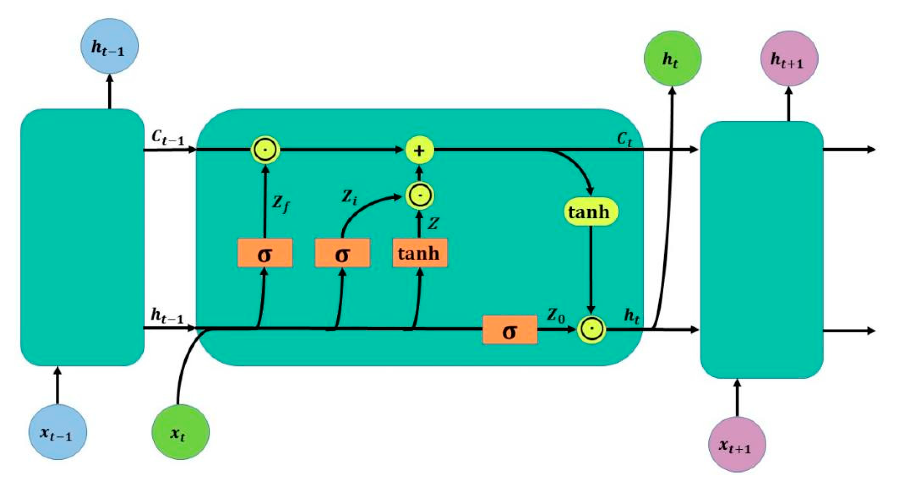
The LSTM neural network introduces a self-loop on top of the RNN, which allows the model to capture long-range dependencies and nonlinear information (Liu et al., 2020). The LSTM neural network contains an input layer, one or more hidden layers, and an output layer, where the hidden layer introduces “input gate”, “forget gate”, and “output gate” control gates. The structure of LSTM is shown in Figure 1.
In this figure, ⊙ represents the Hadamard product of the matrix, i.e., the corresponding elements of the operation matrix are multiplied, and ⊕ represents the performed matrix addition. The calculated Zf (f for forget) is the forget gating, and Zi (i for information) is the selection gating. The results obtained from the above two steps are summed to obtain the Ct transmitted to the next state. The output stage is mainly controlled by Z0 and the Ct obtained in the previous stage is deflated (changed by a tanh activation function) to finally obtain the output ht of the current state. The specific calculation process is as follows.
First, xt and ht−1 passed from the previous state are used as the current input, and the two are trained by LSTM splicing to obtain the following four states:
Among them, Zf, Zi, and Z0 represent a gating state by multiplying the splicing vector by the weight matrix and then converting it to a value between 0 and 1 by the activation function sigmoid. Z is taken as input data and converted to a value between 1 and −1 using the tanh activation function. The two activation functions are calculated as follows:
The next four states are specifically calculated as follows:
Compared with the traditional recurrent neural network, the long short-term memory network model controls the transmission state by gating the state and is able to perform selective memory and interaction within the time series, which is well suited to solving the problem of non-stationarity and randomness of precipitation time series.
2.3. Least Squares Support Vector Machine (LSSVM)
The support vector machine (SVM) is a novel learning approach proposed by Vapnik [22], and mainly adopts the working principle of structural and empirical risk minimization by taking a function metric with low sensitivity, inputting it inside the space, and using the mapping function of the function to map it into a multidimensional space and using linearization in the multidimensional space to solve problems related to low-dimensional nonlinearization. LSSVM is a new machine problem solving method proposed by Suykens et al. [23], and is an upgrade of SVM. It mainly converts the inequality constraint of the traditional SVM into an equation constraint, and at the same time, treats the SSE loss function as the empirical loss of the training set, so that the original solution of the quadratic programming problem can be turned into the solution. This can improve the efficiency of solving the problem on the one hand, and improve the convergence accuracy on the other hand, which can largely reduce the difficulty of the problem from an objective point of view. This not only effectively improves the learning efficiency, but also largely reduces the cost required for computation.
The LSSVM prediction model can be expressed as:
In the equation, the kernel space mapping function is denoted by φ(x); the weights are denoted by w; the training data sets are denoted by T; and the amount of deviation is denoted by b. According to the risk minimization principle, the specific LSSVM data optimization model is shown as follows:
The relaxation factor is denoted by ξ in the equation, when the number of samples reaches the criteria of i = 1, 2,…, N. The Lagrangian function is specified as follows:
where αi is the Lagrangian multiplier. When , , and , it can represent the best conditions for KKT, and w and ξ in the model can be eliminated, resulting in the equation shown below:
In the equation, when , the Mercer condition as a function of K (xi, xj) and the RBF is chosen as the kernel function of the LSSVM, as shown below:
The LSSVM model can be solved as follows:
2.4. Mann–Kendall Test
Before dividing the precipitation data into training and testing sets, it is necessary to identify any change points in the sequence to avoid any interference with the model during the partitioning process. The Mann–Kendall test is a suitable method for determining if there are any change points in the precipitation sequence. If change points are identified, the Mann–Kendall test can also determine the time of occurrence of the change points.
The Mann–Kendall test is a non-parametric method. Non-parametric tests, also known as distribution-free tests, have the advantage of not requiring the sample to follow a certain distribution and being insensitive to outliers. Specifically, for a time series X with n samples, a rank sequence can be constructed as follows:
The rank sequence Sk is the cumulative count of the number of times when the value at time i is greater than the value at time j. Under the assumption of random independence of the time series, a statistic can be defined as follows:
where UF1 = 0, E(Sk), and Var(Sk) are the mean and variance of the cumulative count Sk, respectively. When x1, x2,…, xn are mutually independent and have the same continuous distribution, they can be calculated using the following formulas:
where UFi is a standardized normal distribution calculated in the order of the time series x1, x2,…, xn. When a given significance level is α, according to the normal distribution table, if |UFi| > Uα, a clear trend change in the sequence is indicated.
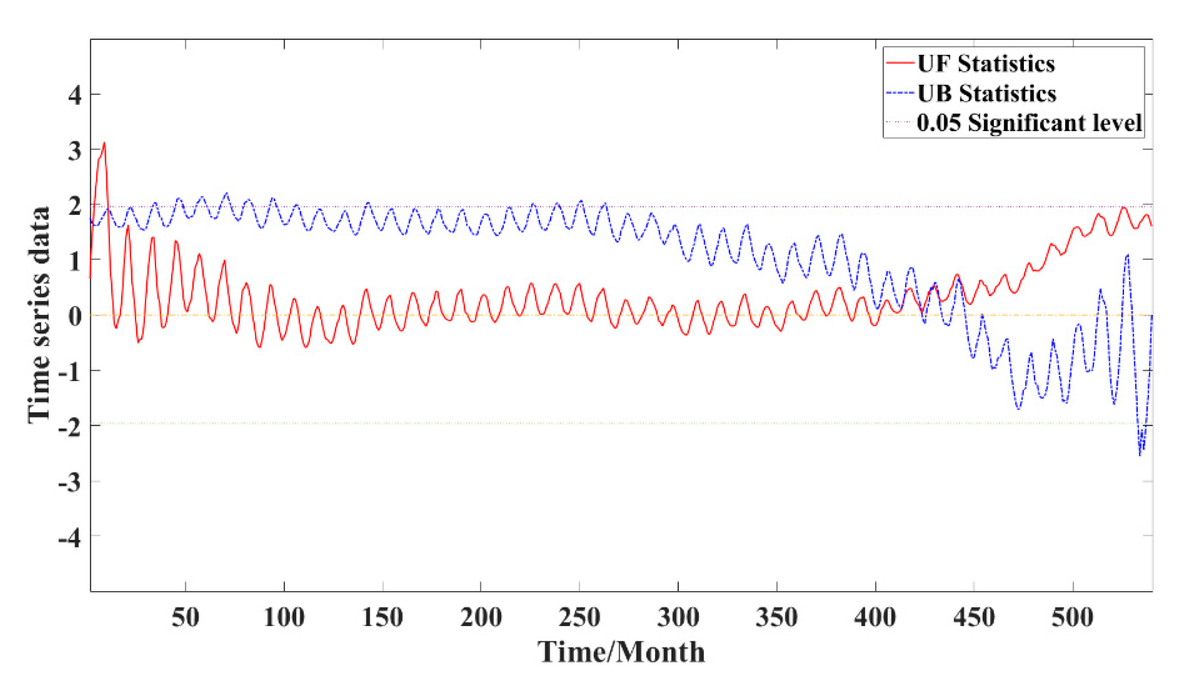
By reversing the time series x to xn, xn−1,…, x1, and repeating the above process while setting UBk = −UFk for k = n, n−1,…, 1 and UB1 = 0, we can obtain a change point detection plot [24]. Among them, the value of UF is greater than zero, indicating that the sequence is in an uptrend, and vice versa. If the two curves of UF and UB intersect between the critical line, the moment corresponding to the intersection point is the time of the start of the mutation. The advantage of this method is that it is not only computationally simple but also able to determine the time when the change point begins and identify the change point region, making it a commonly used method for change point detection.
3. Overview of the Study Area
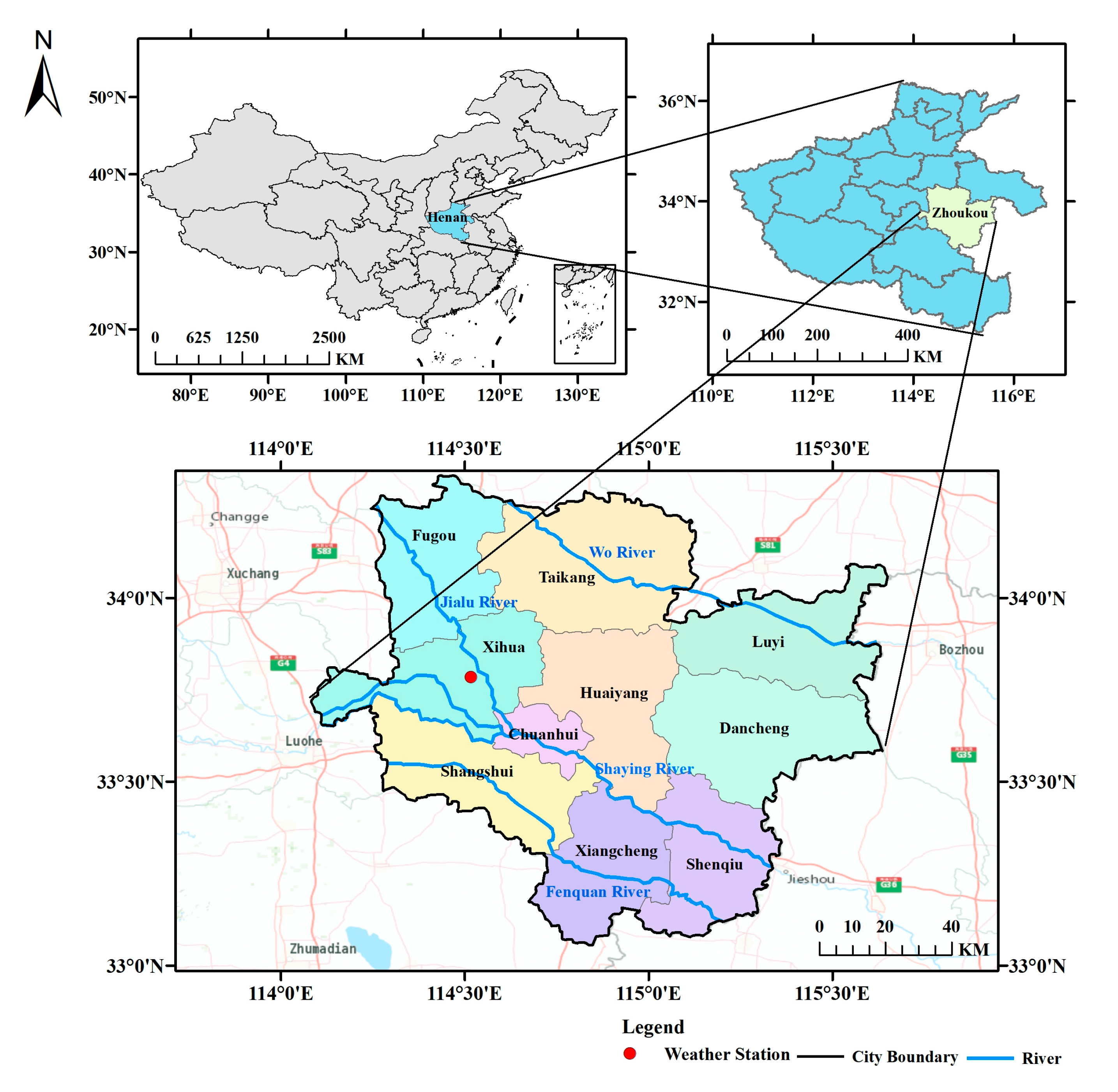
Zhoukou City is located in the central-eastern part of Henan Province, with an area of about 12,000 square kilometers. It is in the middle latitude between the Yellow River and the Huai River, with a flat topography and an elevation between 35.5 and 64.3 m, and belongs to the warm temperate semi-humid semi-arid continental monsoon climate. It is characterized by cold winters and hot summers, rain, and heat in the same period, with an annual average temperature of about 13–22 °C. Daily historical precipitation data were obtained from the National Centers for Environmental Information (https://ngdc.noaa.gov/ (accessed on 20 November 2022)). Longitude and latitude coordinates of weather stations were downloaded from the website, imported into ArcGIS software, and then correlated with the study area to determine the locations of weather stations situated within the study area. The location of the weather station in the study area is illustrated in Figure 2.
Zhoukou is influenced by the alternating effect of the cold Mongolian high and the Pacific sub-high atmospheric flow in winter and summer, respectively, and the intra-year distribution of precipitation in the city is extremely unbalanced. The obtained daily historical precipitation data from the National Centers for Environmental Information (https://ngdc.noaa.gov/ (accessed on 20 November 2022)) website were initially checked and controlled by the article authors. Data with erroneous values, such as single-day precipitation readings of 99.99, were removed. Subsequently, an analysis and collation of the data enabled the calculation of the multi-year average rainfall data for Zhoukou City between 1978 and 2022. Additionally, the multi-year average annual precipitation for each region in China was downloaded from the China Meteorological Data Network (https://data.cma.cn/ (accessed on 20 November 2022)), and annual precipitation raster data for China were obtained via ArcGIS software and the kriging interpolation method [25].
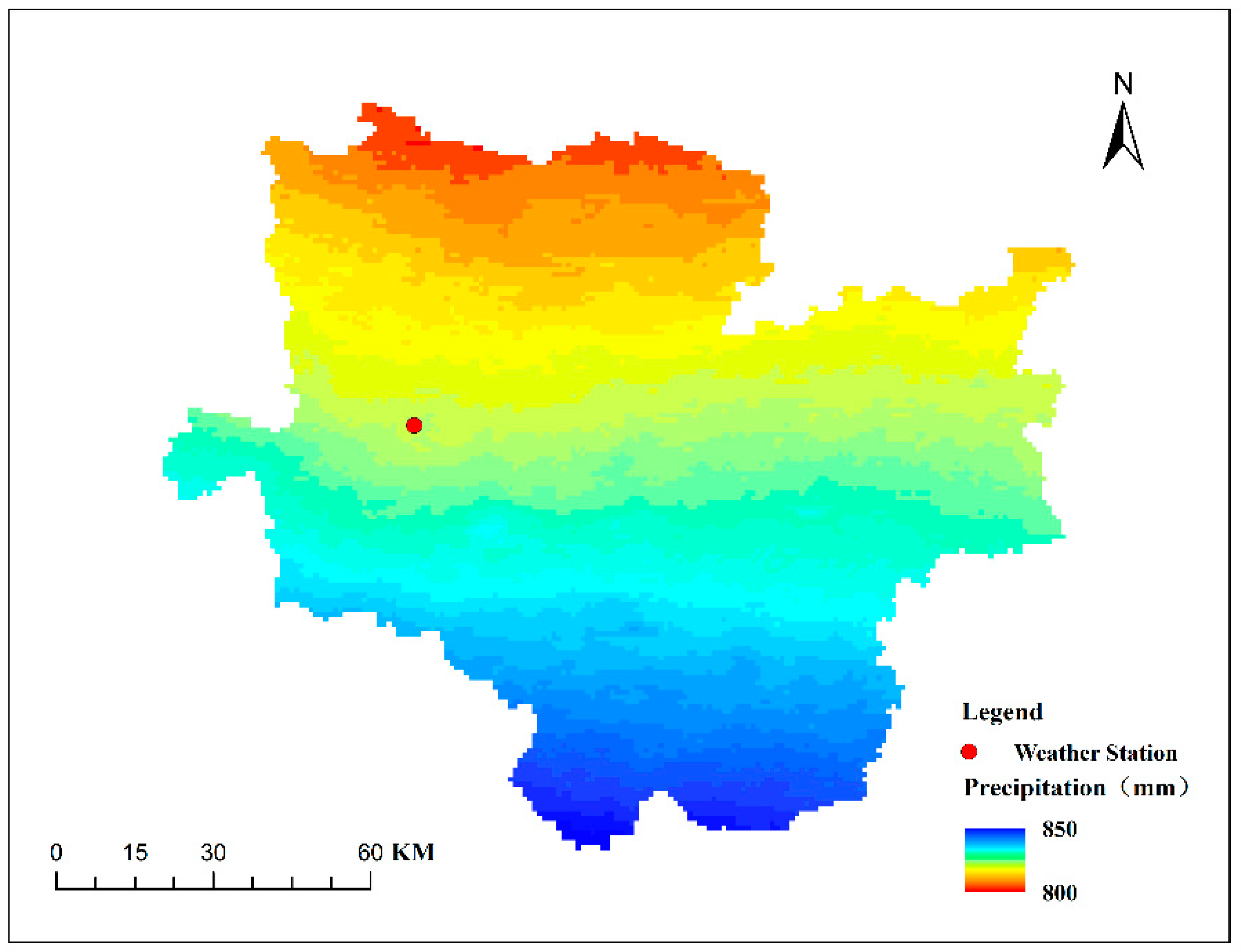
The study utilized the two data products to calculate and validate the annual aver-age rainfall data for Zhoukou City. Through this process, a multi-year average rainfall of 833.47 mm was determined for Zhoukou City. The seasonal average rainfall was also calculated, with the following values obtained: 172.76 mm in spring (March to May), 431.12 mm in summer (June to August), 174.1 mm in autumn (September to November), and 55.49 mm in winter (December to February). Figure 3 illustrates the multi-year average precipitation distribution in the study area, generated via the “Extract by mask” tool in the Spatial Analyst of ArcGIS software after obtaining the annual precipitation raster data for China.
4. Model Building
4.1. Modeling Process
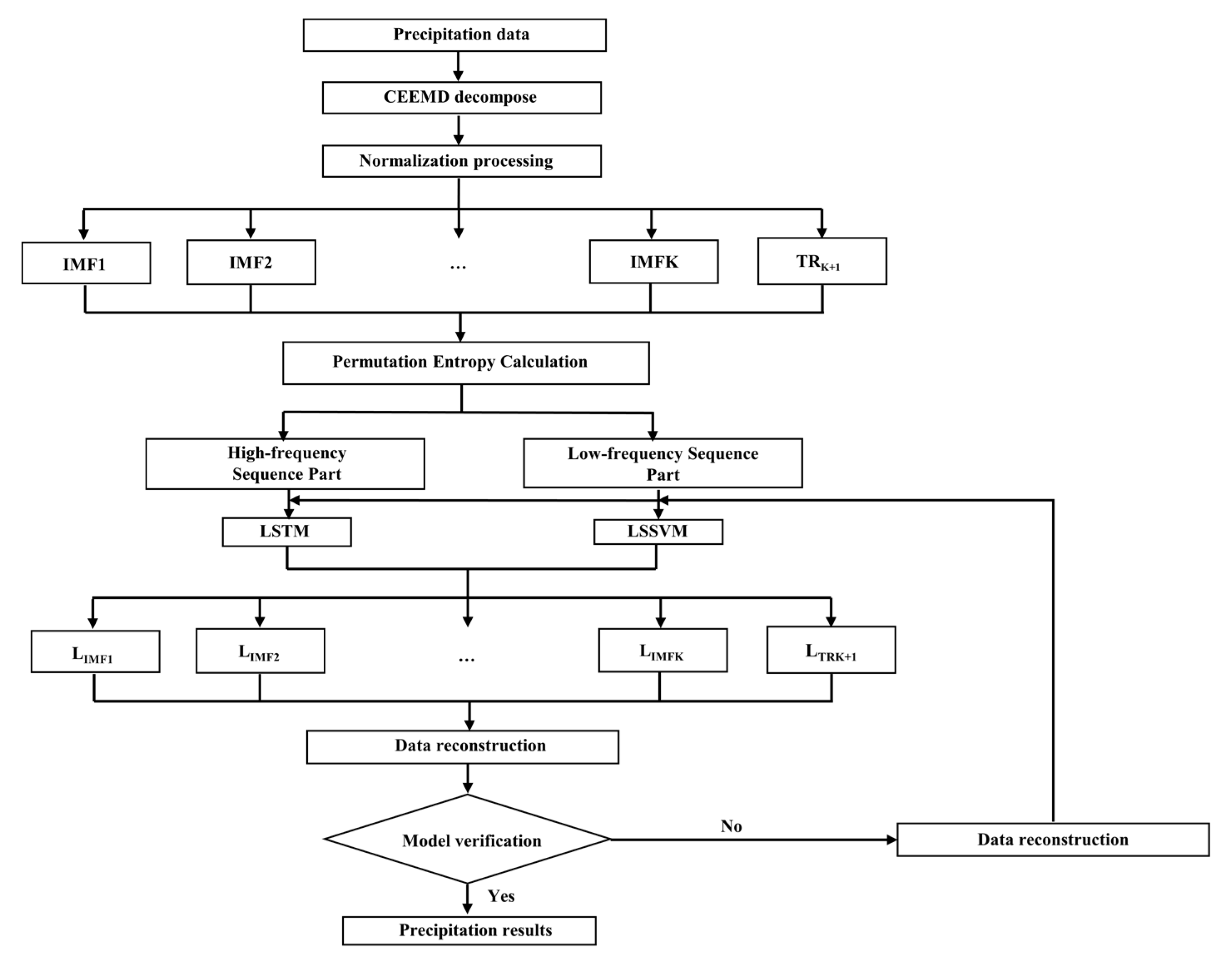
The study is based on the historical precipitation data of Zhoukou City from 1978 to 2022. Firstly, the precipitation series were decomposed by CEEMD to obtain several IMF components and a trend term. Then the components were divided into a high-frequency series part and a low-frequency series part, and a suitable prediction model was constructed based on the Python language environment. Finally, the predicted values of all components were summed to obtain the predicted value of precipitation. The model building process is shown in Figure 4. The specific steps are as follows.
- CEEMD decomposition: The rainfall time series are decomposed by CEEMD to obtain K eigenmodal components and one residual term (trend term).
- Data pre-processing: If the decomposed data are used directly as the input term of the prediction, it will generate large errors, so the entire sample data needs to be normalized.
- To determine the training and prediction sets, the monthly precipitation data of Zhoukou City from 1978–2017 are used as the training data set of the prediction model after decomposition by the CEEMD method; similarly, the monthly precipitation data from 2017–2022 are used as the prediction data set of the forecast after decomposition by CEEMD. Then the Permutation Entropy of the IMF component is calculated, dividing the high and low frequencies.
- Model training: Each set of training input data and prediction data is put into the model for training, and the model input parameters are continuously adjusted so that the model is fully trained on the training data set to ensure that the error is at a low level and to improve the prediction accuracy.
- Model prediction: The prediction is performed using the coupled model, and then the results are inverse normalized and reconstructed, and the final prediction is obtained by superimposing the data according to the principle of superimposing the data at the same moment.
- Accuracy evaluation: The evaluation indicators of the model are calculated and compared with other selected models.
4.2. Model Evaluation Indicators
To measure the prediction accuracy of the model, the root mean square error (RMSE), mean absolute error (MAE), and coefficient of determination (R2) are used as evaluation indicators, where RMSE and MAE are prediction error measures. The smaller the value of these two performance indicators, the closer they are to the actual value. In addition, the closer the value of R2 to 1, the better the fit of the prediction model. The specific equations are as follows:
where yi is the actual value of precipitation at moment i, is the predicted value of precipitation at moment i, and N is the total length of the precipitation series.
4.3. Model Input
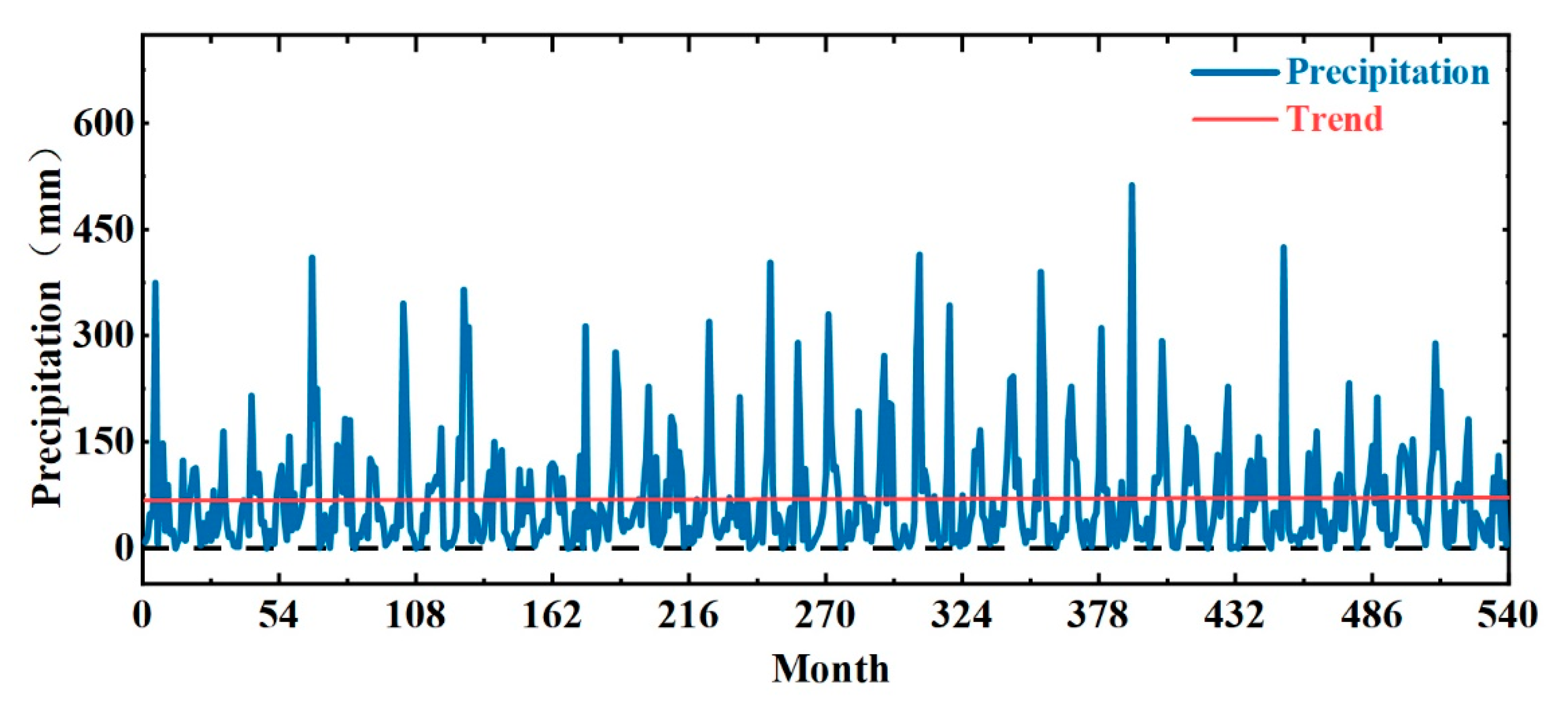
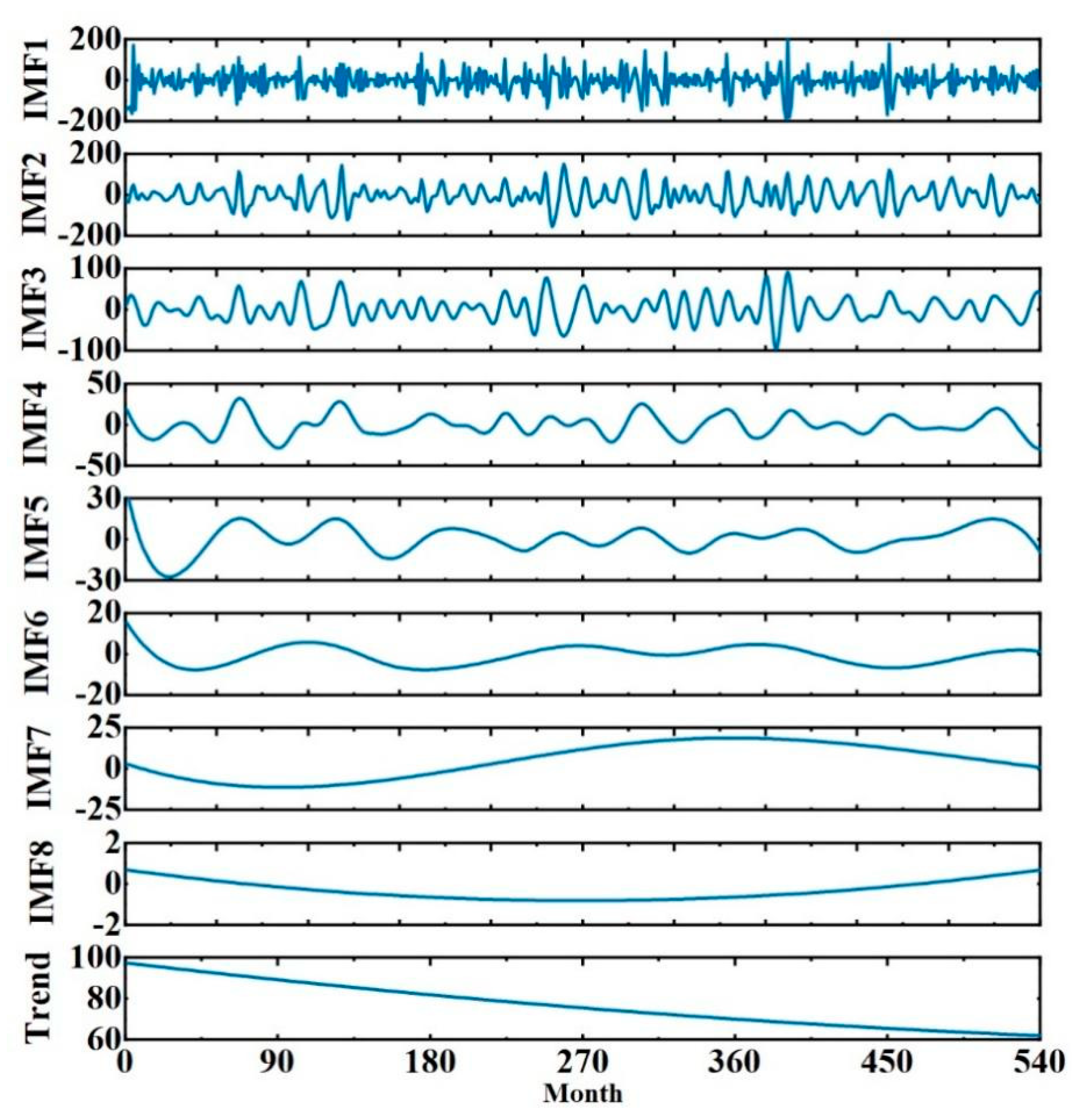
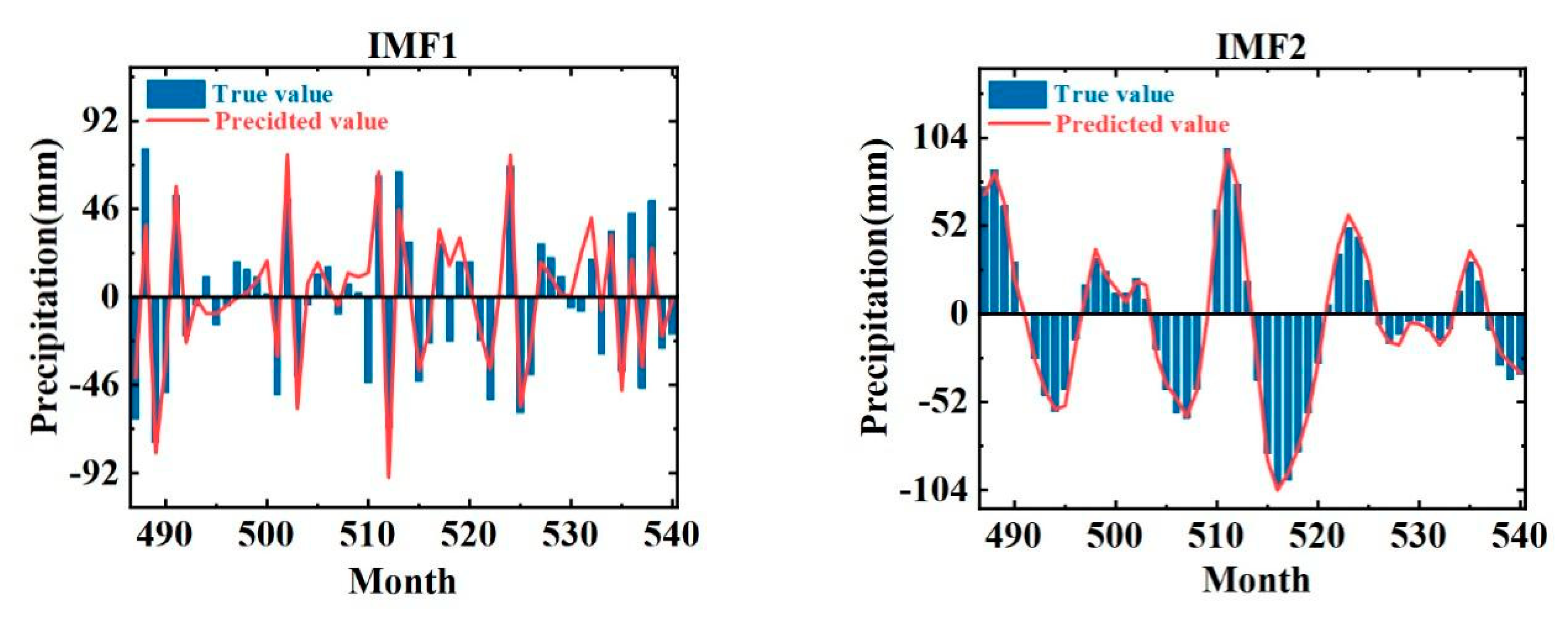
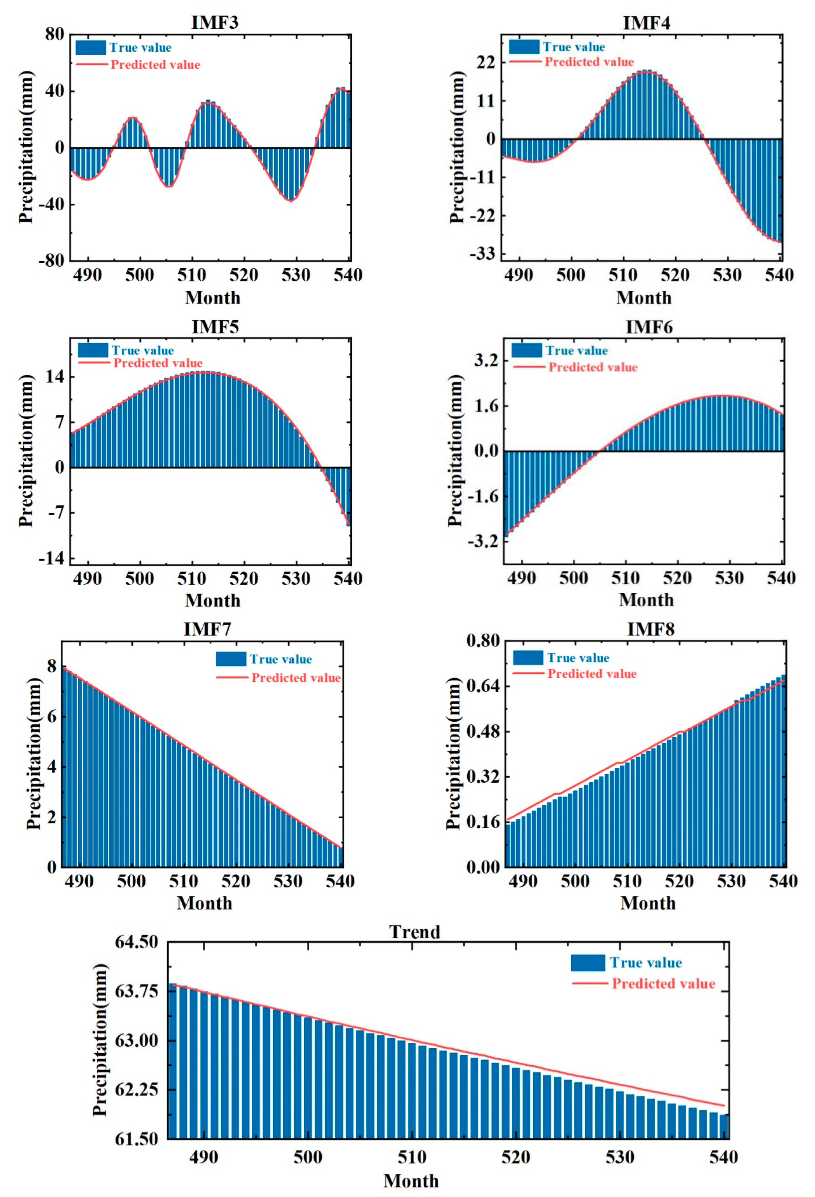
The monthly precipitation of Zhoukou City from 1978 to 2022 is decomposed using the CEEMD model, and Figure 5 shows the monthly precipitation data of Zhoukou City from 1978 to 2022. Then, eight modal components and a residual term (trend term) are obtained. The eight modal components decrease in frequency, and the residual reflects the overall trend of precipitation data, as shown in Figure 6.
As can be seen in Figure 6, the frequencies and amplitudes of the IMF1 and IMF2 components are still at a high level but with less fluctuation and more smoothing than the original data. The frequencies and amplitudes of IMF3–8 decrease gradually with the trend term, and the series gradually tends to be smoother.
Table 1 shows the monthly precipitation series and its decomposition results for Zhoukou City. From the data in the table, the standard deviation of each component is smaller than the standard deviation of the original precipitation series, indicating that the components are less volatile and closer to the mean. In addition, the skewness and kurtosis of the raw precipitation series are larger, indicating that the raw precipitation data are distributed asymmetrically and have more extreme values. In contrast, the skewness values of IMF2, 3, 4, 6, and 8 are close to 0, indicating that their distributions are approximately symmetric; the skewness values of IMF1, 5, 7, and the trend term are around 1, and their distributions have obvious trends when combined with the decomposition plots. In addition, the kurtosis of the decomposed components is much smaller than that of the original data, indicating that the data are less volatile and have fewer extreme values. Therefore, CEEMD is an effective data decomposition method, and the decomposition results can provide more stable input to the coupled model.
The high- and low-frequency sequences were divided with the PE (Permutation Entropy) algorithm, and the high- and low-frequency sequences were then used as the input of different models. The practice was to calculate the perturbation entropy of each sequence; generally speaking, the smaller the perturbation entropy value, the lower the time complexity. The calculation results are shown in Table 2. Among them, the trend terms are used as low-frequency series and predicted using the LSSVM model; IMF1~IMF8 are used as high-frequency series and predicted using the LSTM network model.
4.4. Model Training
Based on the obtained division results, the decomposition result sequence was normalized, and subsequent construction of an LSTM model for each high-frequency sequence and an LSSVM network model for the low-frequency part was performed. Additionally, the M–K test diagram was created via the Mann–Kendall test method, as detailed in Section 2.4. Figure 7 displays the M–K test diagram.
The study utilized a specific method to divide the precipitation data into a training set and test set. From the 540 months of precipitation data, the first 486 items were designated as the training samples, and the last 54 items were used as prediction samples. The component LSTM model was constructed in turn using this approach. The study then employed a step-by-step prediction method of dividing the training–test set to predict each component.
The LSTM model was built on the Python platform and contains several hidden cell layers and dropout layers with a dropout probability of 0.5. The activation function uses tanh, the loss function is mean square error, and the solver is ‘adam’ (adaptive moment estimation). At the same time, since the parameter settings have a significant influence on the accuracy of the LSTM network prediction results, the model needs to focus on the number of nodes in the hidden layer, the number of training times, the learning rate, etc. After successive attempts, the parameters corresponding to the optimal LSTM model are shown in the following Table 3, and the parameters K and α of LSSVM were experimentally judged to be set to 8 and 10, respectively.
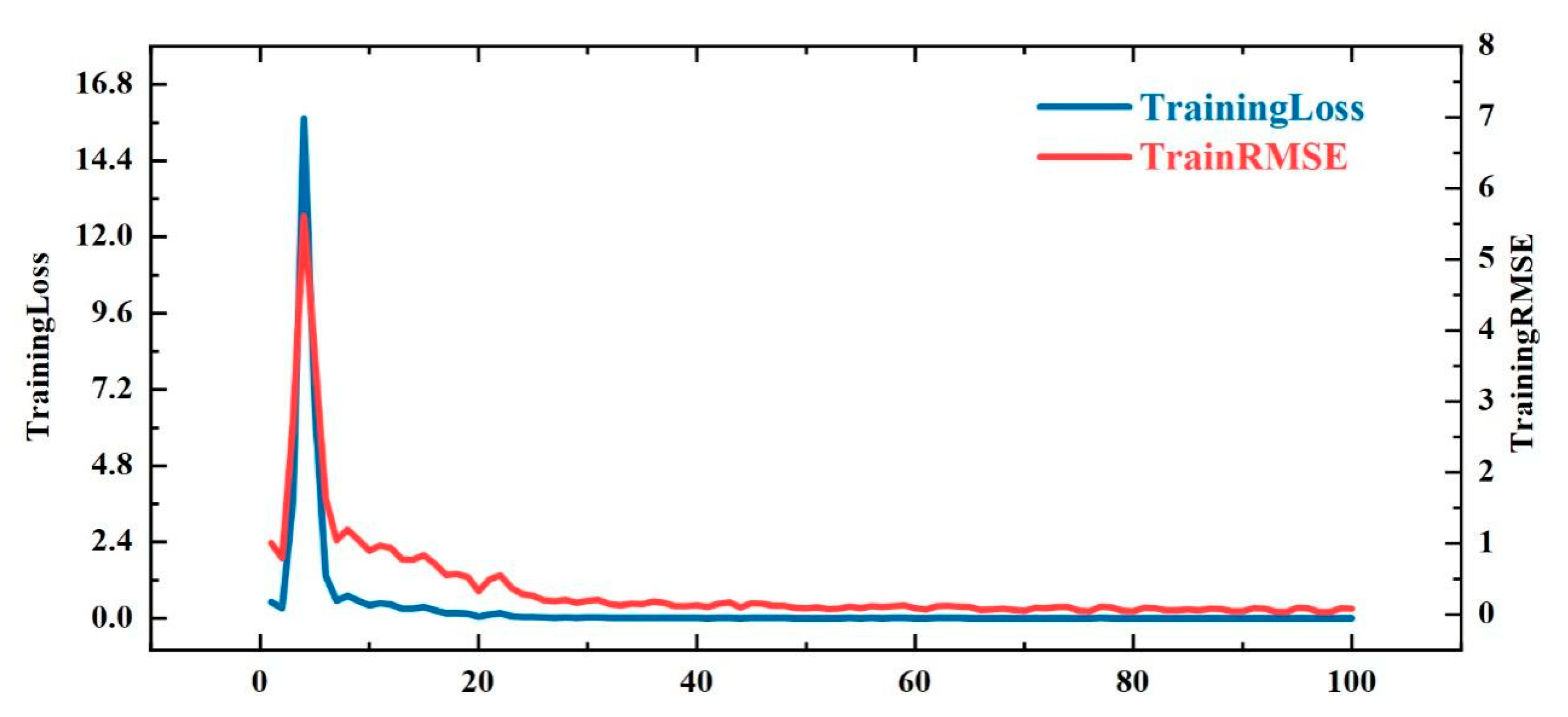
Take the training-prediction process of IMF5 as an example, with an initial learning rate of 0.008, a maximum number of iterations of 100, a gradient threshold of 1, and a hidden node of 130. The specific training process is shown in Figure 8.
As can be seen in Figure 8, the training loss values decrease rapidly within the first 20 steps, indicating a rapid learning rate, and both RSME and training loss values reach stability at 80 steps and drop rapidly to very low levels, indicating that the LSTM is well trained.
5. Analysis and Discussion
After the prediction of the constructed CEEMD-LSTM-LSSVM coupled model, the data need to be inverse normalized to obtain the component prediction values, and Figure 9 shows the comparison of each component series with the observed values after inverse normalization. After calculation, the average relative errors of IMF1–8 are shown in Table 4.
Among them, the average relative errors of IMF1 and 2 are larger, which is due to their larger frequencies. The average relative error from IMF1 to the trend term gradually decreases, and combined with Figure 9, it can be seen that the predicted values of each component basically match with the true values. Therefore, after CEEMD preprocessing, the LSTM model is better for IMF1-IMF8 prediction and the LSSVM model is better for trend terms.
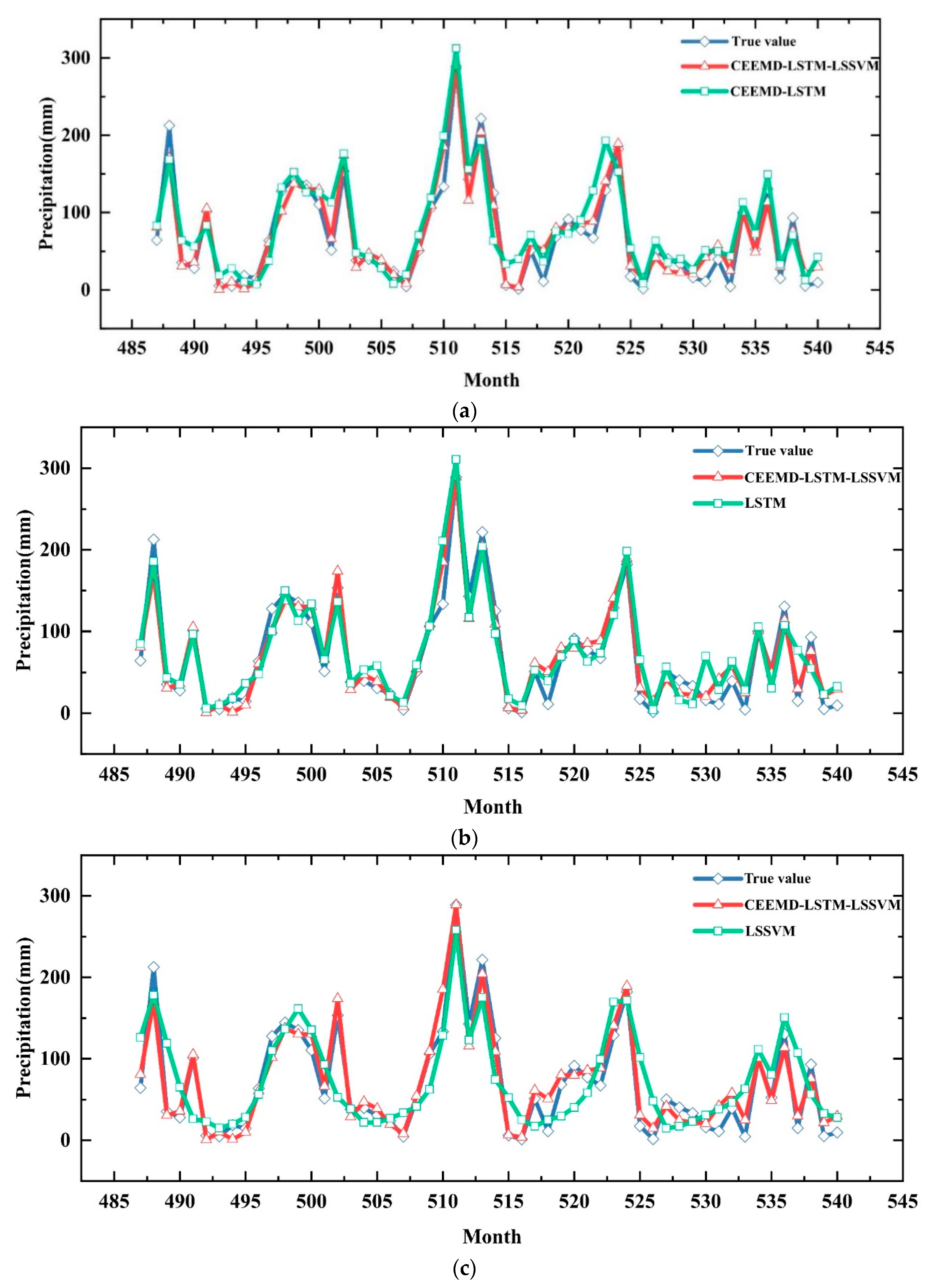
The predicted values of all components and trend terms were summed to obtain the predicted values of monthly precipitation in Zhoukou City, and the prediction results of LSTM, LSSVM, and CEEMD-LSTM models were selected to compare with this model to verify the prediction effect of the CEEMD-LSTM-LSSVM model. The comparison of the prediction results of different models is shown in Figure 10a–c, and the prediction accuracy statistics of different models are shown in Table 5.
As can be seen in Figure 10, all four models provide an overall picture of the general trend of precipitation over the month, but the single LSSVM model does not provide enough detail compared to the measured results, e.g., the prediction error increases rapidly for some months with high precipitation because the strong randomness of the precipitation series interferes with the model prediction accuracy. However, due to the special nature of precipitation prediction, the focus is more on the extreme precipitation events which are more hazardous. The prediction results of the LSTM model are not only closer to the measured results for the months with more precipitation than the LSSVM model, but also have more details for the rest of the months, because the LSTM model can better handle the gradient disappearance and gradient explosion during the long series training process and thus has better performance [26]. The CEEMD-LSTM model also has better prediction results than LSTM and is closer to the measured values in the months with more precipitation, indicating that the decomposition of the precipitation series can improve the accuracy of the model. CEEMD-LSTM-LSSVM has the best prediction results, even in months with high precipitation, because CEEMD completely separates the different fluctuation features in the precipitation series and decomposes the added noise to reduce the reconstruction error [27]. The PE algorithm is then used to divide the high- and low-frequency sequences, and the LSTM model is used to calculate the high-frequency data and the LSSVM model is used to calculate the low-frequency sequences. This allows the model to better capture the variation characteristics of each component, avoiding the situation that a single model produces large errors on inapplicable sequences, and effectively improving the prediction accuracy.
As can be seen from Table 5, the RMSE of the coupled CEEMD-LSTM-LSSVM model is 16.77 mm, the MAE is 13.07 mm, and the R2 is 0.932. The smaller values of these two performance indicators, RSME and MAE, indicate that the predicted value is closer to the actual value and the error of prediction is smaller; the closer R2 to 1, the better the fit of the prediction model. Therefore, the coupled model developed in the article has the highest accuracy compared to the selected comparison model and can be used for the prediction of actual precipitation in the study area.
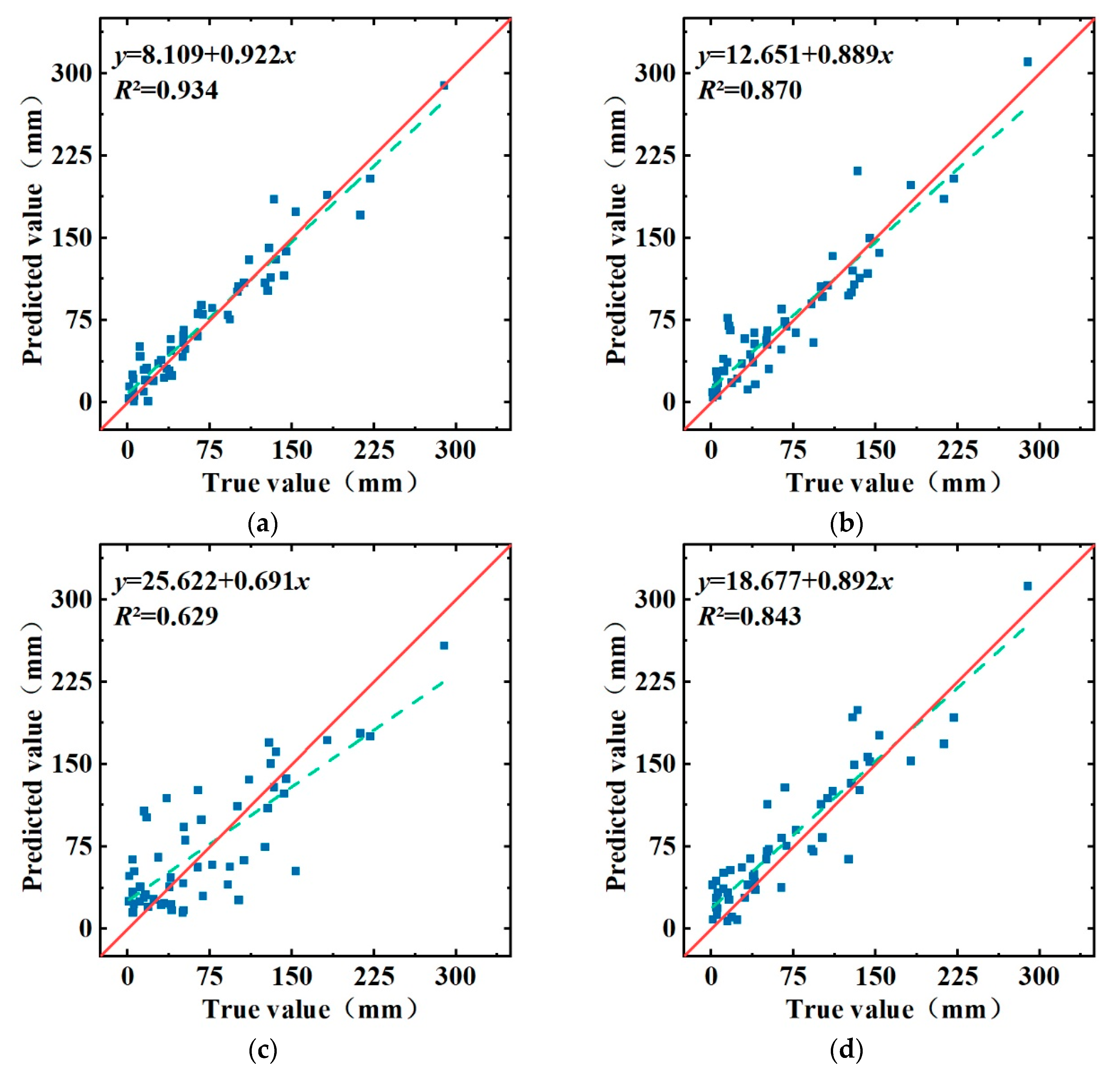
In addition, the scatter plot of the observed and predicted precipitation values can show the distribution of the prediction results of different models and the observed precipitation values more clearly and intuitively. The solid line in Figure 11 is the diagonal line, and the dashed line is the linear fit of the predicted and observed precipitation values of the model. From the distribution of data points in Figure 11, we can find that the data points of the LSSVM model are scattered, indicating that the strong randomness of the precipitation series interferes with the model prediction accuracy. The CEEMD-LSTM model has a better overall prediction accuracy for precipitation, but there are some deviations in the prediction of normal precipitation. The LSTM model has higher prediction accuracy for normal precipitation, but it has a skewed prediction value for rainfall in months with little rainfall. The data points of the CEEMD-LSTM-LSSVM model are almost all distributed on the diagonal, indicating that the model is more accurate in predicting precipitation. The linear fit of the model predictions to the observed precipitation values shows that the R2 of the CEEMD-LSTM-LSSVM model is closest to 1, which indicates that the model predictions are more consistent with the observed precipitation values.
6. Monthly Precipitation Forecasts
The coupled model was used to forecast the rainfall data of Zhoukou City from 2023 to 2025, and the data are shown in Table 6. The historical average precipitation data in the table were obtained by accumulating and then averaging the corresponding months of the collected precipitation data of Zhoukou City from 1978 to 2022, which has some practical significance for evaluating the forecast data.
Among the predicted monthly precipitation data in Zhoukou City, three months in 2023 are lower than the historical average monthly precipitation and nine months are higher than the historical average monthly precipitation; five months in 2024 are lower than the historical average monthly precipitation and seven months are higher than the historical average monthly precipitation; and four months in 2025 are lower than the historical average monthly precipitation and eight months are higher than the historical average monthly precipitation. In addition, the predicted precipitation in July 2024 is the maximum of the past three years, reaching 270.31 mm, which is in line with the precipitation pattern of Zhoukou City in the same period of rain and heat. In addition, combined with the analysis of historical monthly precipitation, precipitation in Zhoukou City is often high in the summer, while in winter the precipitation is low. This pattern is in line with Zhoukou City winter and summer seasons, respectively. Because of the Mongolian cold high and the Pacific paramount atmospheric alternation, the city precipitation distribution within the year is extremely unbalanced.
The study’s results indicate a tendency for the cumulative value of rainfall to increase from 2023 to 2025. This increase in rainfall poses a particular threat to the safety of Zhoukou City during periods of extreme precipitation, such as in July and August. Therefore, Zhoukou City should take corresponding preventive measures against extreme precipitation to improve its flood warning level and risk emergency management. Additionally, urban municipal infrastructure should be strengthened to prevent river flooding and urban flooding caused by heavy rainfall. It is also essential to pay attention to possible drought disasters during the winter season due to low precipitation, which may threaten agriculture and the ecological environment, as well as increase the risk of forest fires.
7. Conclusions
Because of the advantage that the signal decomposition method of the EMD class can directly start decomposition for a period of unknown signals without performing pre-analysis and research, this study performed CEEMD decomposition for the monthly precipitation series of Zhoukou city from 1978 to 2022. This effectively overcame the problems of modal confusion caused by EMD decomposition and large reconstruction errors caused by adding a single white noise to EEMD decomposition. By analyzing the skewness and kurtosis of the decomposition results, this study also proved that the components are more stable and regular compared with the original series, thereby providing a good basis for subsequent prediction. Meanwhile, the PE algorithm was used to divide each modal component into a high-frequency sequence part and a low-frequency sequence part, and the LSTM and LSSVM models were used to predict the two parts, respectively. This reduced the error of each component’s prediction and improved the overall prediction accuracy. The coupled model can thus be used for the prediction of long-term precipitation sequences.
In addition, a coupled CEEMD-LSTM-LSSVM model was developed and applied to month-by-month precipitation forecasting in Zhoukou City. The results show that the coupled model has advantages over the single LSTM neural network model for long series forecasting; the coupled model can portray the actual changes of precipitation series in more detail, and it can also better simulate months in which there are sudden changes in precipitation. Compared with the CEEMD-LSTM, LSTM, and LSSVM models, the RMSE of the predicted data set was reduced by 29.12%, 39.61%, and 59.61%, MAE was reduced by 26.81%, 41.81%, and 57.92%, and the coefficient of determination R2 was increased by 0.08, 0.14, and 0.47, respectively. This indicates that the coupled model proposed in this paper is applicable to monthly precipitation prediction, improves the accuracy of prediction, and can be applied to data analysis and prediction in related fields as a time-frequency domain analysis method.
The overall prediction accuracy of the coupled model proposed in this paper is high. However, the prediction model does not consider the physical conditions that have a large impact on the actual precipitation. In future research, we can try to include meteorological variables such as temperature, air pressure, relative humidity, and wind speed in the model to further improve the prediction accuracy.
Author Contributions
All authors contributed to the study conception and design. Writing and editing: J.C. and Z.G.; chart editing: Y.T.; preliminary data collection: C.Z. and Y.L. All authors have read and agreed to the published version of the manuscript.
Funding
The paper is supported by the National Natural Science Foundation of China (Grant No. U22A20237) and the Open Research Fund of Key Laboratory of Sediment Science and Northern River Training, the Ministry of Water Resources, China Institute of Water Resources and Hydropower Research (Grant No. IWHR-SED-202103).
Data Availability Statement
Datasets and other materials are available with the authors and may be accessible at any time upon request.
Conflicts of Interest
The authors declare no conflict of interest.
References
- IPCC. Impacts of 1.5 °C of Global Warming on Natural and Human Systems; IPCC: Geneva, Switzerland, 2018; Volume 187. [Google Scholar]
- Chen, J.L.; Huang, R.H. Interannual interdecadal variability of water vapor transport in Asian summer winds in relation to droughts and floods in China. J. Geophys. 2008, 2, 352–359. [Google Scholar]
- Zhou, T.J.; Yu, R.C. Atmospheric water vapor transport associated with typical anomalous summer rainfall patterns in China. J. Geophys. Res. 2005, 110, D08104. [Google Scholar] [CrossRef] [Green Version]
- Hossain, I.; Rasel, H.M.; Imteaz, M.A.; Mekanik, F. Long-term seasonal rainfall forecasting: Efficiency of linear modelling technique. Environ. Earth Sci. 2018, 77, 280. [Google Scholar] [CrossRef]
- Jiang, W.; Liu, R.Y.; Chen, P.; Zhang, Z.W. Objective prediction method of summer precipitation in Jiangsu using deep neural network and precursor signal. J. Meteorol. 2021, 79, 1035–1048. [Google Scholar]
- Han, Y.; Guan, J.; Cao, Y.C.; Luo, J. Application of LSTM-WBLS model in daily precipitation prediction. J. Nanjing Univ. Inf. Eng. 2023, 1–10. Available online: https://kns.cnki.net/kcms/detail/32.1801.N.20221111.1728.004.html (accessed on 20 November 2022).
- Narayanan, P.; Basistha, A.; Sarkar, S.; Sachdeva, K. Trend analysis and ARIMA modelling of pre-monsoon rainfall data for western India. Comptes Rendus-Géoscience 2013, 345, 22–27. [Google Scholar] [CrossRef]
- Zhao, Y. Application analysis of gray prediction model for rainfall in Shenwo Reservoir. China Water Energy Electrif. 2016, 12, 68–70. [Google Scholar]
- Gou, Z.J.; Ren, J.L.; Xu, M.; Wang, M. Application of Hadoop-based GA-BP algorithm in precipitation prediction. Comput. Syst. Appl. 2019, 28, 140–146. [Google Scholar]
- Shen, H.J.; Luo, Y.; Zhao, Z.C.; Wang, H.J. Research on summer precipitation prediction in China based on LSTM network. Adv. Clim. Chang. Res. 2020, 16, 263–275. [Google Scholar]
- Wang, R. Research on spatial distribution of rainfall in Handan City based on GIS and support vector machine model. Water Sci. Eng. Technol. 2020, 2, 1–4. [Google Scholar]
- Sha, S.K. Precipitation prediction model based on random forest algorithm in Chengaai irrigation area. Water Resour. Technol. Superv. 2020, 5, 134–137. [Google Scholar]
- Du, K.J. Improved Recurrent Neural Network Method and Its Application Research. Master’s Thesis, Northeastern Electric Power University, Jilin, China, 2021. [Google Scholar]
- Xu, N.N. Research on LSTM-Based ERA5 Day-Scale Precipitation Prediction Method for Mainland China. Master’s Thesis, Nanjing University of Posts and Telecommunications, Nanjing, China, 2021. [Google Scholar]
- Wang, W.C.; Yang, J.X.; Zang, H.F. Monthly precipitation prediction based on WD-COA-LSTM model. J. Water Resour. Water Eng. 2022, 33, 8–13+23. [Google Scholar]
- Yu, Y.H.; Zhang, H.B.; Singh, V.P. Forward Prediction of Runoff Data in Data-Scarce Basins with an Improved Ensemble Empirical Mode Decomposition (EEMD) Model. Water 2018, 10, 388. [Google Scholar] [CrossRef] [Green Version]
- Huang, N.E.; Shen, Z.; Long, S.R.; Wu, M.C.; Shih, H.H.; Zheng, Q.; Yen, N.-C.; Tung, C.C.; Liu, H.H. The Empirical Mode Decomposition and the Hilbert Spectrum for Nonlinear and Non-stationary Time Series Analysis. Proc. R. Soc. A Math. Phys. Eng. Sci. 1998, 454, 903–995. [Google Scholar] [CrossRef]
- Li, D.; Xue, H.F.; Zhang, Y. A combined precipitation prediction model based on empirical modal decomposition. Comput. Simul. 2019, 36, 458–463. [Google Scholar]
- Wu, Z.; Huang, N.E. Ensemble Empirical Mode Decomposition: A Noise-Assisted Data Analysis Method. Adv. Adapt. Data Anal. 2009, 1, 1–41. [Google Scholar] [CrossRef]
- Yeh, J.R.; Shieh, J.S.; Huang, N.E. Complementary Ensemble Empirical Mode Decomposition: A Novel Noise Enhanced Data Analysis Method. Adv. Adapt. Data Anal. 2010, 2, 135–156. [Google Scholar] [CrossRef]
- Roushangar, K.; Alizadeh, F. Scenario-based prediction of short-term river stage–discharge process using wavelet-EEMD-based relevance vector machine. J. Hydroinformatics 2019, 21, 56–76. [Google Scholar]
- Vapnik, V.N. Statistical Learning Theory; John Wiley, Inc.: New York, NY, USA, 1998. [Google Scholar]
- Suykens, J.A.K.; Vandewalle, J. Least Squares Support Vector Machine Classifiers. Neural Process. Lett. 1999, 9, 293–300. [Google Scholar] [CrossRef]
- Huang, H.Y.; Li, E.J.; An, J.; Huang, G.; Bai, Z.N.; Li, D.W. Comparative analysis of precipitation mutation test by Kramer method and Mann-Kendall method. Mod. Agric. Sci. Technol. 2018, 8, 2. [Google Scholar]
- He, H.Y.; Guo, Z.H.; Xiao, W.F. Estimation of monthly precipitation on the Tibetan Plateau using GIS and multivariate analysis. J. Ecol. 2005, 11, 141–146. [Google Scholar]
- Graves, A. Supervised sequence labelling with recurrent neural networks. Stud. Comput. Intell. 2012, 2, 42–45. [Google Scholar]
- Luo, S.X.; Zhang, M.L.; Nie, Y.M.; Jia, X.N.; Cao, R.H.; Zhu, M.T.; Li, X.J. Monthly precipitation prediction in Zhengzhou City based on CEEMDAN-LSTM model. Water Resour. Plan. Des. 2022, 2, 45–50. [Google Scholar]
Figure 1.
Schematic diagram of LSTM structure.

Figure 2.
Location of Zhoukou City.

Figure 3.
Annual average precipitation distribution in the study area from 1978 to 2022.

Figure 4.
Flow chart of CEEMD-LSTM-LSSVM coupling model.

Figure 5.
Month-by-month precipitation data for Zhoukou City, 1978–2022.

Figure 6.
CEEMD decomposition results of month−by−month precipitation in Zhoukou City for 1978–2022.
Figure 6.
CEEMD decomposition results of month−by−month precipitation in Zhoukou City for 1978–2022.

Figure 7.
M−K test plot of rainfall data in the study area.

Figure 8.
Training loss and RMSE values of IMF3.

Figure 9.
Comparison of the predicted results of IMF1–8 and trend terms with the measured values.


Figure 10.
Comparison of prediction results of the CEEMD-LSTM-LSSVM model with those of other models. (a) Prediction results of CEEMD-LSTM-LSSVM compared with CEEMD-LSTM. (b) Comparison of prediction results of CEEMD-LSTM-LSSVM with LSTM. (c) Comparison of prediction results of CEEMD-LSTM-LSSVM and LSSVM.

Figure 11.
Scatterplot of observed and predicted precipitation values. (a) CEEMD-LSTM-LSSVM. (b) CEEMD-LSTM. (c) LSTM. (d) LSSVM.
Figure 11.
Scatterplot of observed and predicted precipitation values. (a) CEEMD-LSTM-LSSVM. (b) CEEMD-LSTM. (c) LSTM. (d) LSSVM.


Table 1.
Statistics of raw precipitation and decomposition results.
| Rainfall Sequence | Min Value (mm) | Max Value (mm) | Average Value (mm) | Standard Deviation (mm) | Skewness | Kurtosis |
|---|---|---|---|---|---|---|
| Original sequence | 0.00 | 512.06 | 69.46 | 79.13 | 5.66 | 2.16 |
| IMF1 | −194.27 | 201.66 | −5.62 | 52.25 | 1.51 | −0.12 |
| IMF2 | −154.73 | 150.99 | −5.62 | 50.29 | 0.04 | 0.14 |
| IMF3 | −96.53 | 92.15 | 0.21 | 28.46 | 0.36 | 0.25 |
| IMF4 | −29.78 | 32.25 | −0.61 | 12.43 | −0.23 | 0.16 |
| IMF5 | −27.40 | 35.63 | 0.47 | 9.21 | 1.10 | −0.51 |
| IMF6 | −7.70 | 15.21 | −0.71 | 4.34 | −0.56 | 0.07 |
| IMF7 | −11.31 | 18.74 | 4.85 | 10.38 | −1.41 | −0.18 |
| IMF8 | −0.82 | 0.68 | −0.32 | 0.45 | −0.85 | 0.64 |
| Trend | 61.87 | 97.31 | 76.81 | 10.33 | −1.11 | 0.32 |
Table 2.
Trend of IMF components and trend term entropy after CEEMD decomposition.
| Rainfall Sequence | Displacement Entropy | Rainfall Sequence | Displacement Entropy | Displacement Entropy | Displacement Entropy |
|---|---|---|---|---|---|
| IMF1 | 1.8 | IMF4 | 0.85 | IMF7 | 0.68 |
| IMF2 | 1.35 | IMF5 | 0.78 | IMF8 | 0.62 |
| IMF3 | 1.08 | IMF6 | 0.72 | Trend | 0 |
Table 3.
Parameters corresponding to the LSTM model.
| Rainfall Sequence | Number of Nodes in the Hidden Layer | Number of Training Sessions | Learning Rate |
|---|---|---|---|
| IMF1 | 200 | 230 | 0.01 |
| IMF2 | 200 | 200 | 0.01 |
| IMF3 | 150 | 150 | 0.01 |
| IMF4 | 150 | 110 | 0.008 |
| IMF5 | 130 | 100 | 0.008 |
| IMF6 | 130 | 60 | 0.006 |
| IMF7 | 100 | 50 | 0.005 |
| IMF8 | 100 | 35 | 0.005 |
| Trend | 60 | 25 | 0.005 |
Table 4.
Mean relative error of IMF1–8.
| Portion Size | Average Relative Error (%) | Portion Size | Average Relative Error (%) | Portion Size | Average Relative Error (%) |
|---|---|---|---|---|---|
| IMF1 | 94.59 | IMF4 | 5.4 | IMF7 | 2.85 |
| IMF2 | 25.95 | IMF5 | 5.52 | IMF8 | 0.49 |
| IMF3 | 6.74 | IMF6 | 4.27 | Trend | 0.1 |
Table 5.
Prediction accuracy of different models.
| Models | RSME (mm) | MAE (mm) | R2 |
|---|---|---|---|
| CEEMD-LSTM-LSSVM | 16.77 | 13.07 | 0.932 |
| CEEMD-LSTM | 23.66 | 17.86 | 0.864 |
| LSTM | 27.77 | 22.46 | 0.813 |
| LSSVM | 38.92 | 31.06 | 0.633 |
Table 6.
Prediction results of the coupled CEEMD-LSTM-LSSVM model of monthly precipitation in Zhoukou City from 2023 to 2025.
Table 6.
Prediction results of the coupled CEEMD-LSTM-LSSVM model of monthly precipitation in Zhoukou City from 2023 to 2025.
| Year | January | February | March | April | May | June | July | August | September | October | November | December |
|---|---|---|---|---|---|---|---|---|---|---|---|---|
| 2023 | 16.26 | 29.38 | 43.30 | 54.81 | 64.20 | 93.66 | 216.10 | 181.49 | 89.77 | 68.21 | 27.18 | 12.29 |
| 2024 | 15.80 | 27.69 | 41.25 | 53.09 | 65.96 | 115.81 | 270.31 | 134.74 | 89.82 | 57.40 | 24.52 | 14.48 |
| 2025 | 19.76 | 31.65 | 44.89 | 56.92 | 71.65 | 126.32 | 266.02 | 117.23 | 88.56 | 52.17 | 23.12 | 15.36 |
| HistAvg | 16.05 | 20.37 | 34.34 | 50.21 | 88.21 | 87.01 | 197.68 | 146.43 | 83.92 | 56.85 | 33.33 | 19.07 |
Disclaimer/Publisher’s Note: The statements, opinions and data contained in all publications are solely those of the individual author(s) and contributor(s) and not of MDPI and/or the editor(s). MDPI and/or the editor(s) disclaim responsibility for any injury to people or property resulting from any ideas, methods, instructions or products referred to in the content. |
© 2023 by the authors. Licensee MDPI, Basel, Switzerland. This article is an open access article distributed under the terms and conditions of the Creative Commons Attribution (CC BY) license (https://creativecommons.org/licenses/by/4.0/).
Share and Cite
MDPI and ACS Style
Chen, J.; Guo, Z.; Zhang, C.; Tian, Y.; Li, Y. Research on the Application of CEEMD-LSTM-LSSVM Coupled Model in Regional Precipitation Prediction. Water 2023, 15, 1465. https://doi.org/10.3390/w15081465
AMA Style
Chen J, Guo Z, Zhang C, Tian Y, Li Y. Research on the Application of CEEMD-LSTM-LSSVM Coupled Model in Regional Precipitation Prediction. Water. 2023; 15(8):1465. https://doi.org/10.3390/w15081465
Chicago/Turabian StyleChen, Jian, Zhikai Guo, Changhui Zhang, Yangyang Tian, and Yaowei Li. 2023. "Research on the Application of CEEMD-LSTM-LSSVM Coupled Model in Regional Precipitation Prediction" Water 15, no. 8: 1465. https://doi.org/10.3390/w15081465
Note that from the first issue of 2016, this journal uses article numbers instead of page numbers. See further details here.