Article

Numerical Evaluation of the Hydrothermal Process in a Water-Surrounded Heater of Natural Gas Pressure Reduction Plants

by
Hamid Kazemi Moghadam
1,
Seyed Soheil Mousavi Ajarostaghi
1,2,*,
Mohsen Saffari Pour
3,* and
Mohsen Akbary
1
1
Faculty of Mechanical Engineering, Babol Noshirvani University of Technology, Babol 47148-71167, Iran
2
Mechanical Engineering Department, Université de Sherbrooke, Sherbrooke, QC J1K OA5, Canada
3
Department of Mechanical Engineering, Faculty of Engineering, Shahid Bahonar University of Kerman, Kerman 76169-13439, Iran
*
Authors to whom correspondence should be addressed.
Water 2023, 15(8), 1469; https://doi.org/10.3390/w15081469
Submission received: 8 February 2023 / Revised: 22 March 2023 / Accepted: 3 April 2023 / Published: 9 April 2023
(This article belongs to the Special Issue Laminar and Turbulent Flow: Heat and Mass Transfer)

Abstract

:
The gas pressure in the main network of transmission lines is about 700 to 1000 psi (4826.33 to 6894.76 kPa), which is reduced to 250 psi (1723.69 kPa) at the entrance station of a city. This reduction process, which occurs in the regulator, causes a severe drop in gas temperature. The drop in the gas temperature produces hydrates and even causes the water vapor in the gas to freeze. As a result, there is a possibility that the passage of gas in the regulator is blocked and the gas flow is cut off. By employing heaters (indirect water heaters), the temperature of the gas entering the regulator can be preheated to eliminate the possibility of freezing in the regulator. This heater is fueled with natural gas and it operates for 24 hr a day, especially in the cold seasons. Therefore, one of the main challenges in using this type of heater is its high fuel consumption. Consequently, researchers are looking for a solution to reduce the fuel consumption (natural gas) of gas heaters. In this paper, the heat transfer and fluid flow in a heater of a natural gas pressure reduction plant, the Aliabad Power Plant (Iran), are numerically investigated using a commercial Computational Fluid Dynamics (CFD) code, ANSYS FLUENT 18.2. The considered heater consists of three parts, including (i) gas coils, (ii) a water bath (shell), and (iii) a fire tube. The indirect heat transfer process takes place between the hot liquid flow in the fire tube (combustion exhaust) and the cold liquid flow (natural gas) using the natural convection flows generated in the water bath. Numeric modeling is performed for four different gas mass flows, including 6 × 10⁴, 8 × 10⁴, 1 × 10⁵, and 12 × 105 standard cubic meters per hour (or 16.67, 22.22, 27.78, and 33.33 m3/s). The results indicate that the natural gas outlet temperature achieved to a temperature higher than required. By installing a regulator on the burner, the gas consumption can be reduced, resulting in station cost savings, and also reducing the environmental impacts. The outcomes depict that the maximum possible reductions in monthly gas consumption and economic savings in the proposed system are 67,500 m3 and IRR 25 million at a gas mass flow rate of 60,000 SCMH.

1. Introduction

Nowadays, the proper and optimal use of energy in the world is particularly important. One of the most critical energy sources in the world is natural gas, and its use is increasing every year. Its increasing growth and non-compliance with energy consumption standards, both economic and environmental, pose a serious threat to many countries. Natural gas is transported between production and consumption points at high pressures (700–1000 psi or 4826.33 to 6894.76 kPa), and it is necessary to reduce this operating pressure. This can be achieved in natural gas pressure reduction stations, where the pressure is reduced from 800–1000 psi to 250 psi (1723.69 kPa). In natural gas pressure reduction stations, linear heaters immersed in water are used during preheating for safety reasons and to prevent gas explosions. These are the most common type of heaters used in the gas pressure reduction stations, but they have high heat loss. Therefore, increasing heat transfer in heaters used for gas pressure reduction stations results in lower natural gas consumption and improved performance of this type of heater at the lowest cost.
In 2007, Shokouhmand et al. [1] studied the air-to-fuel ratio in the burner of heaters used in pressure-reducing systems. They also compared other heaters with the existing ones. In 2008, Hedman et al. [2] proposed the use of an expansion turbine instead of the existing system. The high-pressure gas enters the turbine and, in addition to reducing the desired pressure, causes the turbine to rotate, resulting in electricity generation. The main problem with this plan is that the gas inlet pressure in the station is not constant. In 2011, Farzaneh et al. [3] used a solar collector system to optimize the heaters of gas pressure reduction stations. The solar system heats the water in the heater to a certain temperature, reducing the fuel consumption of the heater and the running costs. The payback period is estimated at 35 years. In 2011, Clay and Tansley [4] simulated a combined power generation and home-heating system using fluid calculations. They were able to increase the temperature of the combustion products by raising the temperature of the inlet air introduced to the burner using a recuperator, thus recovering the energy wasted by the stack.
In 2011, Howard et al. [5] found a new way of reducing energy use in pressure-reducing systems. They used a hybrid system comprising an expansion turbine and fuel cell to generate electric power in addition to heating the gas, which increased efficiency. In 2014, Andrei et al. [6] attempted to utilize the mechanical energy wasted during gas pressure reduction. They were able to achieve significant results by using expansion turbines instead of pressure relief valves in Ansti, which were experimentally fabricated and resulted in power generation. In 2014, Ashouri et al. [7] calculated the minimum inlet temperature needed in the controller to reduce the energy consumption of heaters. They gathered 10 months of data for the pressure-reducing station of the city of Biston and found good agreement between the collected data and the equation AGA-8. In 2015, Farzaneh and Ghezelbash [8] increased the temperature of the gas inlet in a heater using a geothermal heat exchanger upstream of the pressure-reducing station heater. Their results show that less fuel was needed to heat up the gas, and it was thus an effective method of reduce the greenhouse gases. In 2016, Ghezelbash et al. [9] proposed a new system based on using a vortex tube instead of a pressure relief valve and a geothermal heat exchanger to reduce the energy consumption of a heater. The vortex tube divides the gas stream into cold and hot streams, so that the heated cold stream in the geothermal heat exchanger mixes with the hot steam from the vortex tube and is sent to the heater at low pressure. According to the results, the proposed system can reduce energy consumption by 88 percent. In 2017, Salari and Goudarzi [10] studied the effect of a turbulator as a passive method to increase the heat transfer and thus the heating capacity of Central Gas Supply system (CGS) of Yasuj station. In their study, the effect of using a spring in the tube as a turbulator on the performance of a heater was investigated in two cases, considering circular and elliptical tubes with similar cross-sections. The results show that the tube with the spring with a diameter ratio of 10 had the best performance in the heater with elliptical tubes with a diameter ratio of 0.95.
In 2018, Olfati et al. [11] comprehensively analyzed the energy and exergy characteristics of a natural gas power plant considering seasonal variations and found that most energy losses occur in the stack during winter. In 2018, Naderi et al. [12] tested the water heating system in a gas pressure reduction station in Iran. They used the waste heat from the chimney to heat the water in the heater. The results show that the efficiency of the heater increased due to its lower fuel consumption. This project was conducted at a pressure reduction station in Shahrekord. The results show that the proposed plan reduces the fuel consumption of the heater by about 45%. Economic analysis also shows that the payback period for such a station is about 1.3 years. In 2018, Rahmatpour and Shabani [13] studied the economic and exergetic use of expansion turbines instead of pressure-reducing valves in pressure-reducing stations. Their results show high operating cost and a long payback period. In 2019, Khosravi et al. [14] improved the thermal performance of linear heaters in gas pressure reduction stations. They proposed the use of an alternating current in the gas tubes, which is transferred from the water to the gas tubes, to increase the thermal efficiency of the heater. As a result, the use of heating coils increased the efficiency of the heater. Their work demonstrated an increase in the Nusselt number of 20%, and as a result of this, increased thermal efficiency and reduced fuel usage. In 2019, Noorollahi et al. [15] presented a new system for supplying the required heat to the gas pressure reduction station. To eliminate the consumption of natural gas in linear heating systems, they introduced shell and tube heat exchangers with geothermal pumps. The results show a reduction in greenhouse gases and a 47 percent reduction in CO2 emissions.
In this paper, the heat transfer and fluid flow in a heater of a CGS, located in Aliabad Power Plant (Iran), are numerically studied using a commercial CFD code, ANSYS FLUENT 18.2. The considered heater consists of three parts, including (i) gas coils, (ii) a water bath (shell), and (iii) a fire tube. The indirect heat transfer process takes place between the hot liquid flow in the fire tube (combustion exhaust gas) and the cold liquid flow (natural gas) using the natural convection currents generated in the water bath (jacket of the heater).

2. Materials and Methods

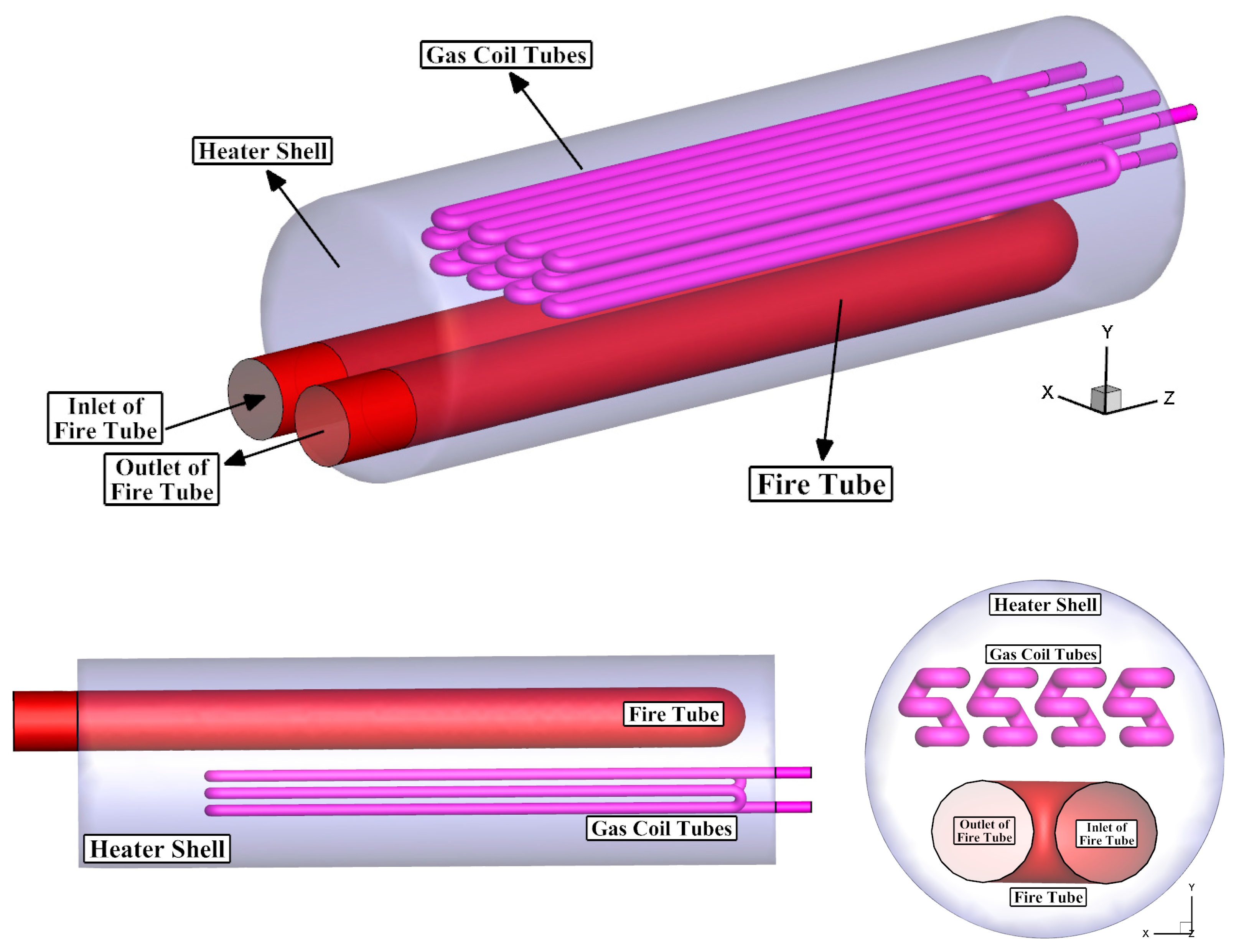
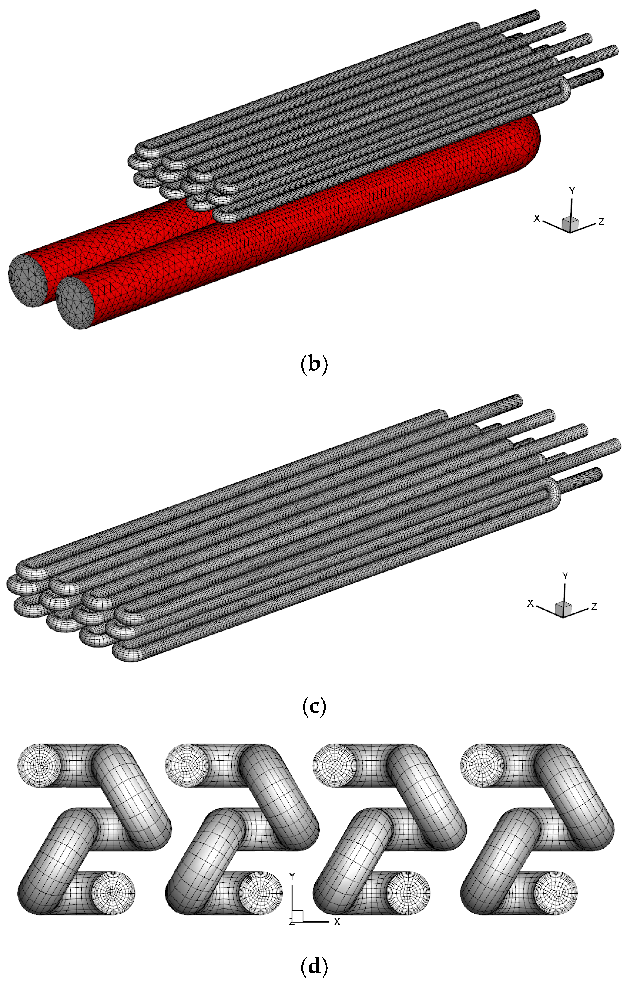
2.1. Geometrical Parameters

The purpose of this study is to numerically model and investigate the heat transfer process in a gas heater of a CGS. The gas heater under consideration is located in the Aliabad Power Plant (Iran). This heater was built in 2003. The capacity of this heater is 120,000 standard cubic meters per hour (SCMH) or 33.33 m3/s; it can absorb 819,500 kcal/h (0.953 kW) with 4 coils. It has eight gas pipes. Coil diameter and length are 4 in (0.1016 m) and 236.22 in (6 m), respectively. Additionally, the operational temperature and pressure of the heater under investigation are 40 °C and 1050 psi (7239.49 kPa), respectively. Moreover, the maximum and minimum burner capacity are 150,000 kCal/h (174.45 kW) and 750,000 kCal/h (827.25 kW), respectively. Furthermore, the fire tube diameter and length are 4 in (0.6 m) and 267.72 in (6.8), respectively.
Due to the complexity of the geometry of the heater, SolidWorks, a powerful tool for design and modeling, was used for geometric modeling, and then the geometry was entered into ANSYS software to perform meshing and modeling. In general, due to the use of an indirect heat transfer mechanism, a gas heater consists of three parts: a fire tube, a shell, and gas coils. The 3D and 2D schematics of the heater under study are shown in Figure 1. As can be seen, the gas enters from one side and leaves from the same side after passing through the hot water bath. In addition, the hot combustion exhaust gases flow into a U-shaped tube, which serves as a fire tube. The heating mantle, which contains hot water and is also called the hot water bath, contains pure water that causes a density difference due to the temperature difference between the surface of the fire tube and the gas coils, creating a natural convection flow.
As can be seen in Figure 1, a total of 4 coils are arranged side by side in such a way that the input and output of the gas flow arrive from a common header. The coils are also interconnected by 4 holding plates (practical). As mentioned earlier, the coil has a diameter of 0.1016 m and a length of about 6 m. To increase the contact area and thus the heat transfer rate, each register has five 180-degree bends. The fire tube is 0.6 m in diameter and approximately 6.8 m in length. The approximate diameter and length of the heater are 2.2 and 6.8 m, respectively.

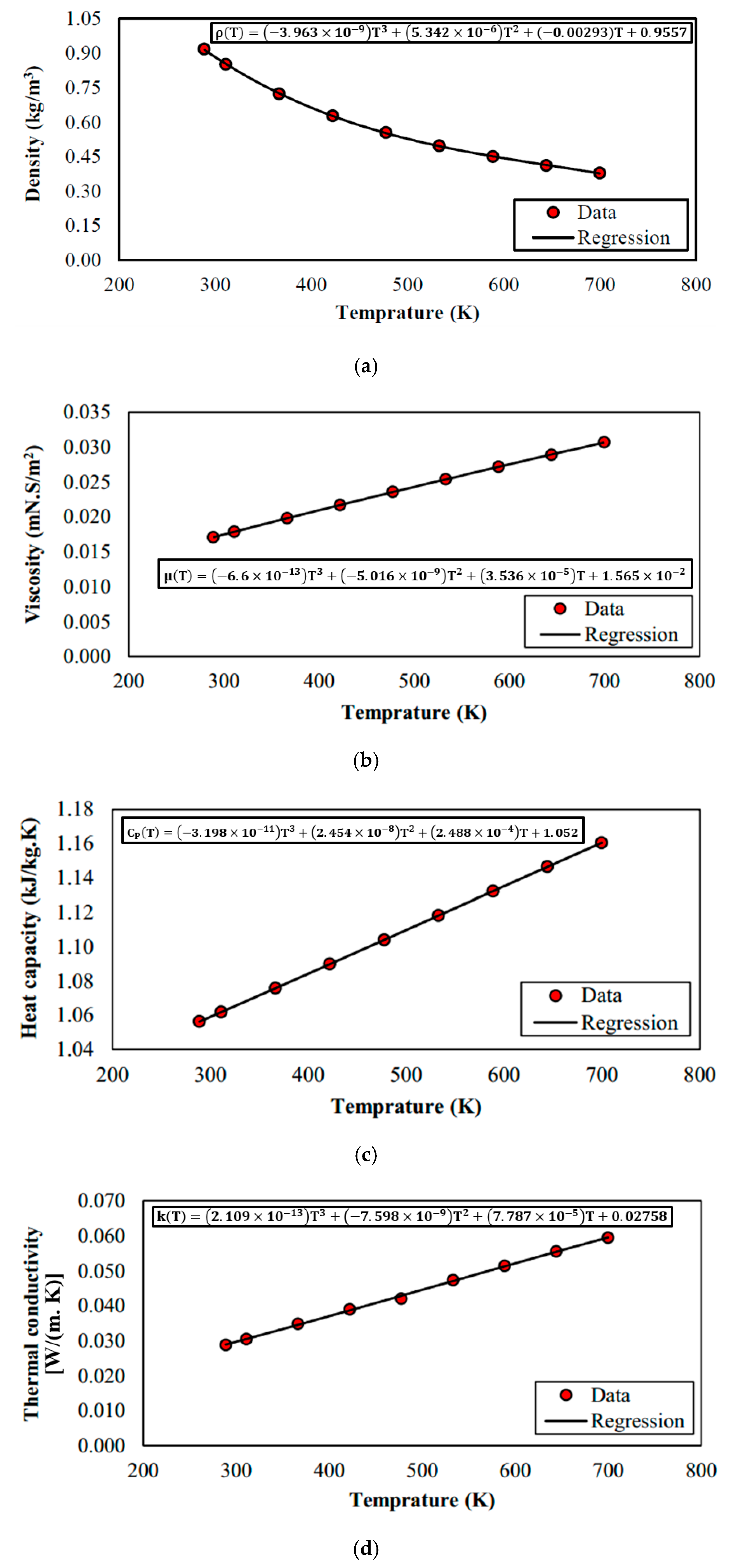
2.2. Governing Equations and Parameters

Computational fluid dynamics (CFD) offers valuable insight into essential transport phenomena, including heat transfer, momentum transfer, and mass transfer. Therefore, CFD provides vital information on the heat transfer and natural convection processes between the working fluid in a fire tube, gas tube, and water tank. Numerous heating, ventilation, and air conditioning (HVAC) equipment manufacturers have turned to CFD simulation to accelerate prototyping and present new designs. CFD simulation allows engineers to study the possible performance of their products in various spaces, and with different configurations [16,17].
The basic equations governing fluid mechanics are all written based on the control mass, and on the other hand, the fluid flow is investigated in the control volume. Therefore, a tool for transformation is needed, which is provided by the general transport equation. Using the general transfer equation, the laws of conservation of mass and linear momentum are written for the control volume of the fluid that moves at an arbitrary velocity, and thus the basic equations governing the flow, continuity, and Navier–Stokes equations are obtained.
In order to analyze a real flow, it is necessary to use basic governing equations, such as continuity, momentum, and energy, as well as complementary equations such as state and turbulence. Considering that most fluid flows are turbulent by nature, in the real and accurate analysis of a fluid flow, it is essential to consider the effects of turbulence in the equations governing the fluid flow. With the view that there is no single model able to consider the effects of turbulence for all flows among the various experimental models that are available to apply the effects of turbulence, appropriate models are employed to analyze this specific turbulence problem. In this section, the basic equations governing the flow field are presented. In the following, the correct and accurate procedure for modeling fluid flow in a numerical solution, considering the effect of turbulence, which plays the most important role in flow modeling, is presented.
Momentum Conservation Equations [18,19,20,21]:
ρ D u D t = ( P + τ x x ) x + τ y x y + τ z x z + S M x
ρ D v D t = τ x y x + ( P + τ y y ) y + τ z y z + S M y
ρ D w D t = τ x z x + τ y z y + ( P + τ z z ) z + S M z
In the above equations, the parameter P is the static pressure on the fluid. Without considering the exact details of the body forces, the overall effect of these forces can be considered as a source term, SMi, for the amount of momentum in the direction i per unit volume and per unit time, where i includes x, y, or z directions. If the body forces only include gravity, which is the case in the present problem, then SMx = SMz = 0 and SMy = −ρg.
In Equations (1)–(3), surface forces can include pressure, viscosity, and body forces such as gravity, centrifugal force, etc. In many fluid flows, viscous stresses may be expressed as functions of the local strain rate. In three-dimensional flows, the local rate of deformation will be a combination of the linear rate of change and the volume rate of change. For incompressible fluids, the mass conservation equation is div U = 0 and the viscous stresses are twice the local rate of linear deformation multiplied by the dynamic viscosity. The momentum equations, which are known as the Navier–Stokes equations, can be written as follows [18,19,20,21]:
( ρ u ) t + d i v ( ρ u U ) = P x + d i v ( μ . g r a d ( u ) ) + S M x
( ρ v ) t + d i v ( ρ v U ) = P y + d i v ( μ . g r a d ( v ) ) + S M y
( ρ w ) t + d i v ( ρ w U ) = P z + d i v ( μ . g r a d ( w ) ) + S M z
In the k-ε turbulence model, the values k and ε are obtained directly from the differential transfer equations of the turbulence kinetic energy and the turbulence dissipation rate, as follows [18,19,20,21]:
( ρ k ) t + ( ρ U k ) = ( ( μ + μ t σ k ) k ) + P k ρ ε
( ρ ε ) t + ( ρ U ε ) = ( ( μ + μ t σ ε ) ε ) + ε k ( C ε 1 ( P k ) C ε 2 ρ ε )
where Pk is the production of turbulence due to viscous forces, which is defined as follows:
P k = μ t U ( U + U T ) 2 3 U ( 3 μ t U + ρ k )
In this turbulence model, the constant coefficients of C μ , C ε 1 , C ε 2 , σ k , and σ ε are equal to 0.09, 1.44, 1.92, 1.0, and 1.3, respectively.
When the wall functions are used, the average velocity, average temperature, k, and ε are all calculated by these functions. So, there is no longer a need to consider the boundary conditions on the walls. The use of wall functions is acceptable for a wide range of problems. When the flow near the wall is strongly affected by the reverse pressure gradient, or when the flow is in a severe non-equilibrium state, then the solutions derived from the standard functions should be doubted. The contour of y+ distribution on the surface of the tube is shown in Figure 2, which shows the acceptable values of y+ in the presented model.
Mass Conservation Equation [18,19,20,21]:
ρ t + ( ρ u ) x + ( ρ v ) y + ( ρ w ) z = 0
ρ t + d i v ( ρ U ) = 0
In the above equations, U and ρ are the velocity vector and fluid density, respectively. Additionally, u, v, and w are the velocity vector components in various axes.
Turbulent Energy Equation [18,19,20,21]:
( ρ u T ) x + ( ρ v T ) y = x [ ( μ l + μ t σ T ) ( T x ) ] + y [ ( μ l + μ t σ T ) ( T y ) ]
μ t = ρ c μ k 2 ε
To include the influence of buoyancy on the water tank side, Boussinesq approximation is employed [22,23]:
ρ = ρ 0 [ β ( T T l i q u i d u s ) + 1 ] 1
in which β is the thermal expansion coefficient. Finally, to calculate the heat flux passing through the coolant tube walls, the following equation based on Fourier’s law is utilized:
δ r = k t u b e d T ( r ) d r

2.3. Boundary Conditions

The temperature of the combustion exhaust varies according to the ratio of fuel to air and is around 800 K. In contrast, the temperature of the gas entering the station varies at different times of the year and is about 280 K. The dimensionless Grashof number (Gr = gβ (TS − T) D32) is used to determine the flow regime in free convection heat transfer. This number indicates whether the flow is laminar or turbulent. The Grashof number is obtained from the ratio of the buoyancy force to the viscous force. In this correlation, the parameters g, β, TS, T, D, and υ express the gravitational acceleration, volumetric expansion coefficient, hot surface temperature, cold surface temperature, length characteristics, and kinematic viscosity, respectively. If the Grashof number is greater than 10 + 8, the flow is turbulent. According to the specifications of this issue, the Grashof number is about 6 × 10 + 6, so the flow regime is laminar. On the other hand, due to the high liquid flow rate inside the fire tube and gas line, the Reynolds number of the flow is much higher than 2300, so the liquid flow is completely turbulent.
Given the known gas volume flow and inlet pressure in the heater, the amount of inlet gas is determined and the Velocity_Inlet boundary condition is used. In this study, simulations were performed for an inlet pressure of 700 psi (4826.33 kPa) and four different inlet volume flow rates. The four flow rates considered in this study were 60,000, 80,000, 100,000, and 120,000 SCMH (or 16.67, 22.22, 27.78, and 33.33 m3/s). The gas inlet temperature in the heater was assumed to be 10 °C according to the ambient conditions. An inlet velocity of 5 m/sec and a temperature of 800 K were assumed for the inlet boundary of the fire tube assuming an additional fuel-to-air ratio of 1.8, an air inlet temperature of 30 °C, and a methane flame temperature of 2400 K at a pressure of 1 bar. The volumetric expansion coefficient of water was assumed to be 0.0005 K−1 to model the effects of natural convection. The gas entering the heater consists of various components with different ratios. Table 1 shows the components of the gas and the volume fraction of each component. As can be seen, about 90% of the gas consists of methane gas, so for simplicity’s sake, only methane gas was considered as a component of the city gas in further modeling processes.
Due to the fact that the gas entering the station at a pressure of 700 psi (4826.33 kPa) is considered, the thermophysical properties of methane gas at the desired pressure and temperature of 20 °C are listed in Table 2.
There combustion exhaust gases are composed of several gases, which are listed in Table 3. As can be seen, combustion produces different types of gas in different volume fractions depending on the amount of burner gas flow. In this study, only one type was considered to simplify the calculation and modeling of the combustion exhaust gas, but the thermophysical properties of the exhaust gas in the burner tube were considered as a function of the gas temperature to avoid errors in the solution process; the history of these functions is shown in Figure 3.

3. Results and Discussion

In this section, numerical modeling results are presented for four different gas mass flows, including 60,000, 80,000, 100,000, and 120,000 SCMH (or 16.67, 22.22, 27.78, and 33.33 m3/s). The results include the outlet temperature of methane and combustion gas, the temperature and velocity distribution in the heater, and the thermal efficiency of the heater.

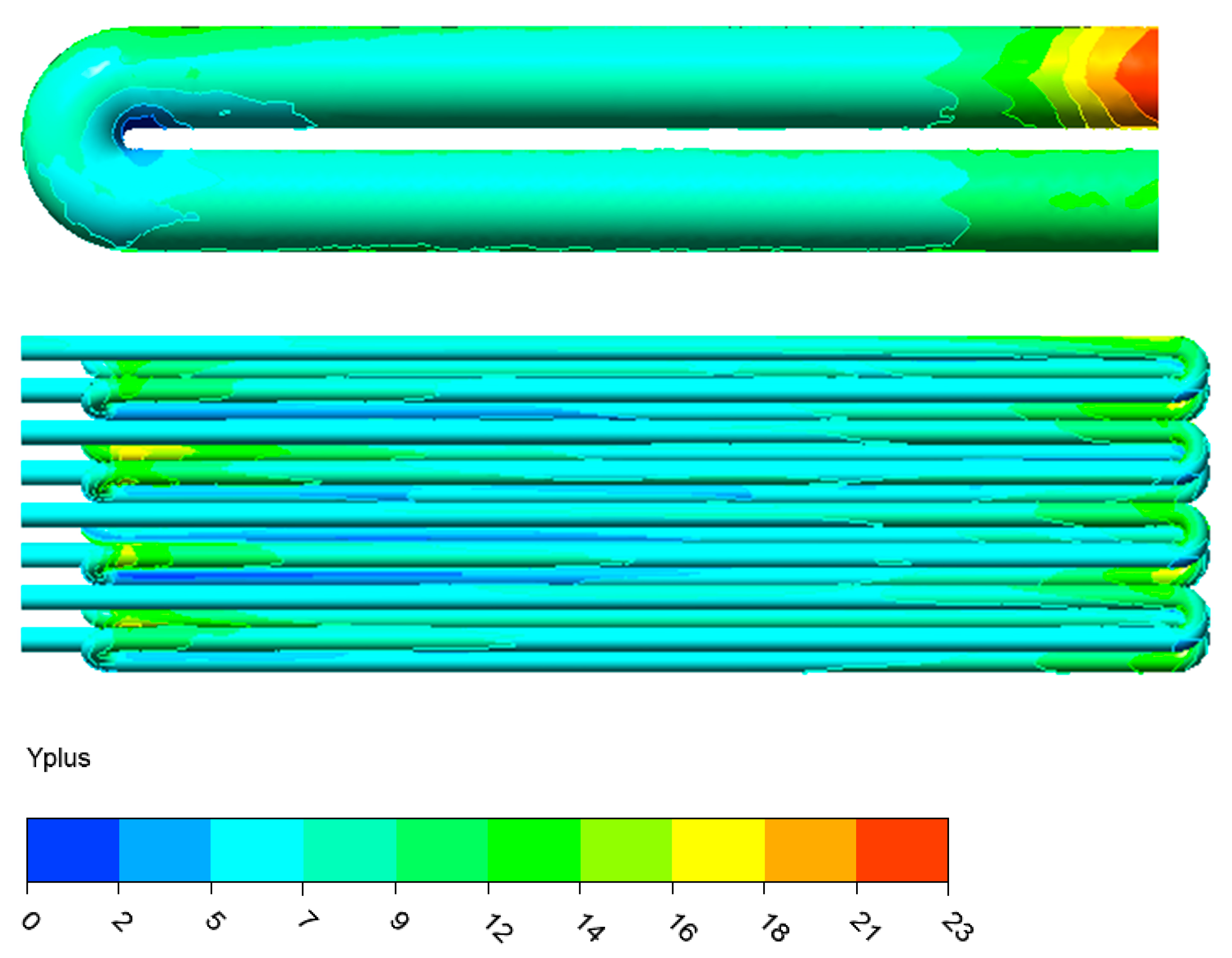
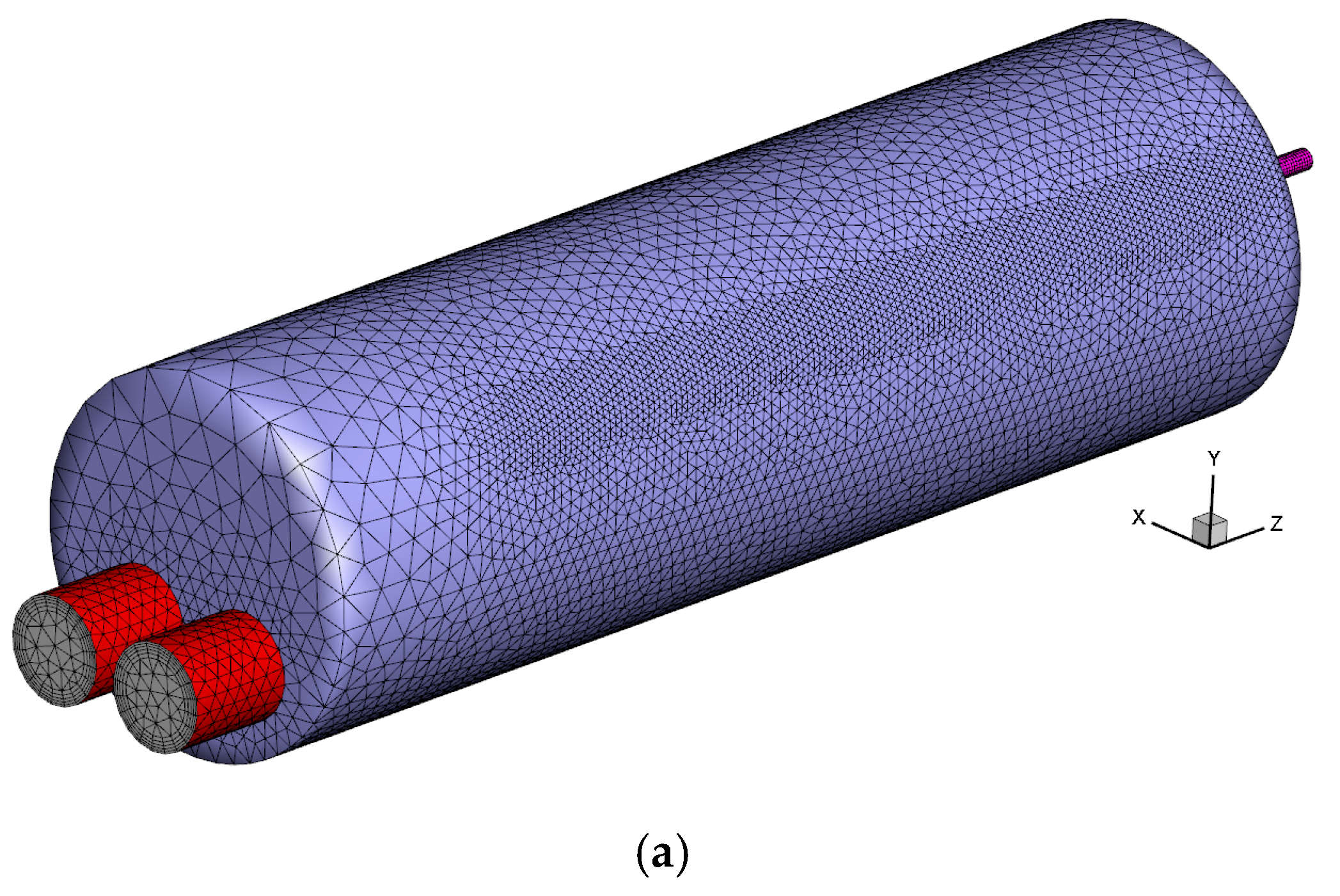
3.1. The Mesh-Independent and Validation Analyses

In any numerical work, checking the independence of the results from the grid and validation analysis is critical. By checking the independence of the results from the grid, the independence of the results considering the number and quality of grids was determined.
Grid generation was performed using ANSYS meshing. A hexagonal grid was used in the coil domain to reduce the computational volume and increase the accuracy of the solution. Five edge layers were generated in the coil region with an initial layer height of 0.5 mm. In the fire tube region, a mesh with a mesh size of 2 cm along the tube and seven layers of boundary layer mesh with a first layer thickness of 0.5 mm were used.
In this study, three different mesh qualities were considered, including 3,708,213, 4,777,825 and 6,210,401 cells, and the results were investigated based on the gas outlet temperature. In this section, the methane volume flow rate considered is 60,000 SCMH (16.67 m3/s). The numerical results obtained for these networks are shown in Table 4. It can be concluded that the grid with 4,777,825 cells is suitable for use in the following sections of this work. Images showing grid generated for the heater under consideration from different perspectives are shown in Figure 4. It can be seen that to increase the accuracy of the numerical simulation, the boundary layer grid was used in both the gas tube and the fire tube.
The validation of the present numerical method was carried out using practical data of a heater of a real gas station. Station data were available for a pressure of 700 psi (4826.33 kPa) and various flow rates, which are listed in Table 5. The comparison of the data from a real gas station and the modeling results presented here shows that the accuracy of the presented numerical model is acceptable considering the simplifying assumptions. It can be seen from Table 5 that the maximum error for the three different gas mass flows was 3.52%.

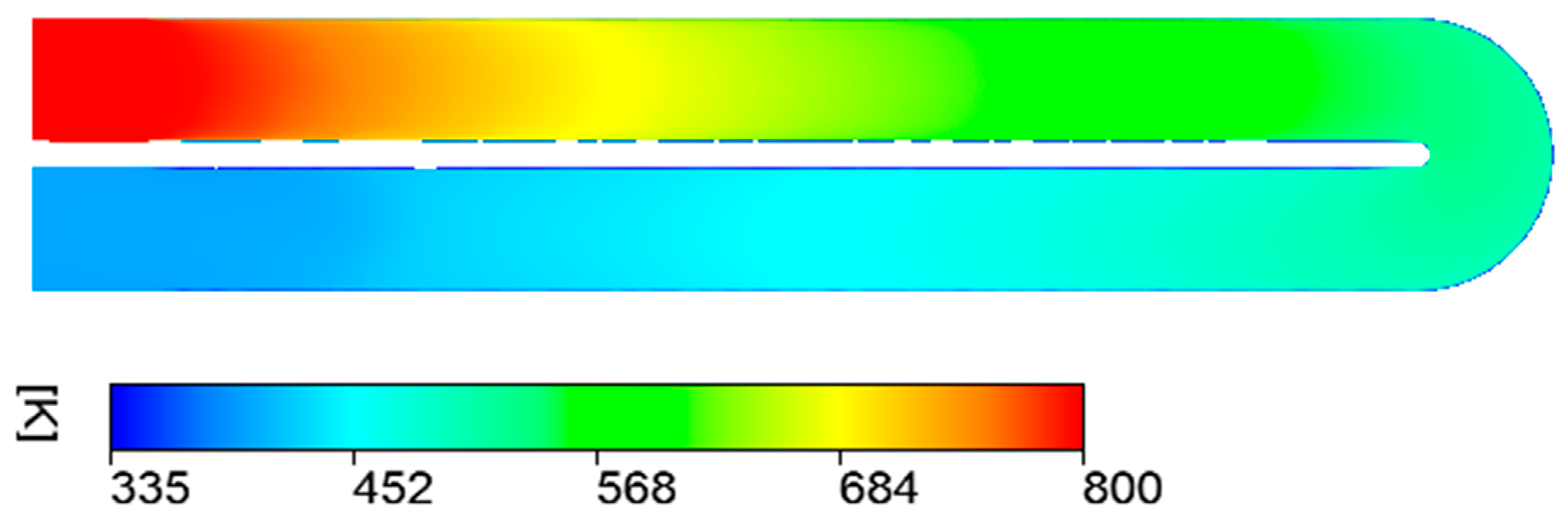
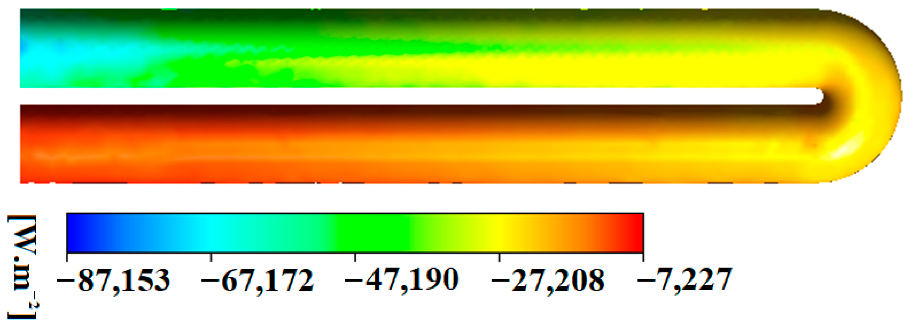
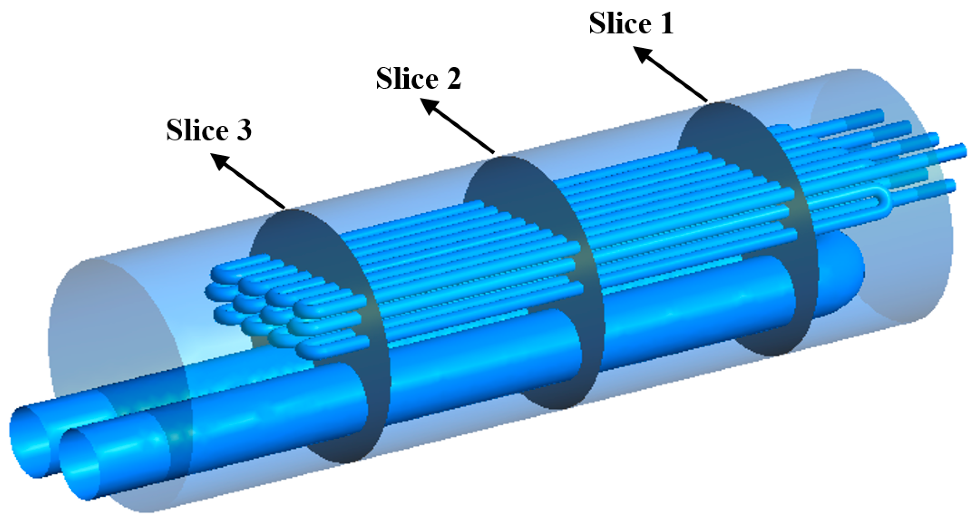
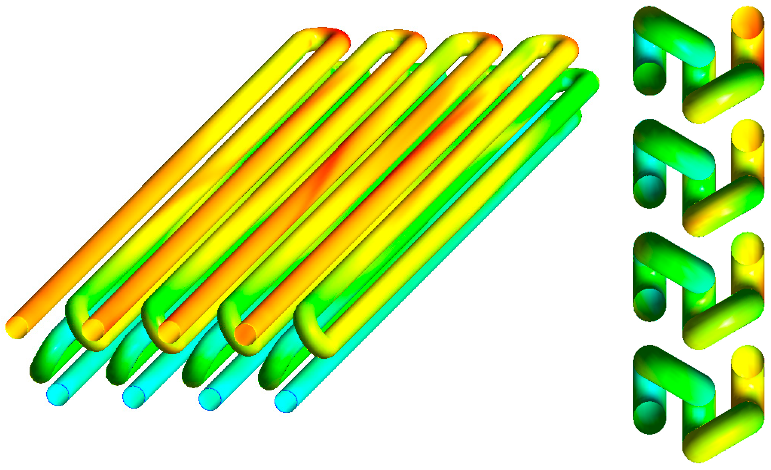
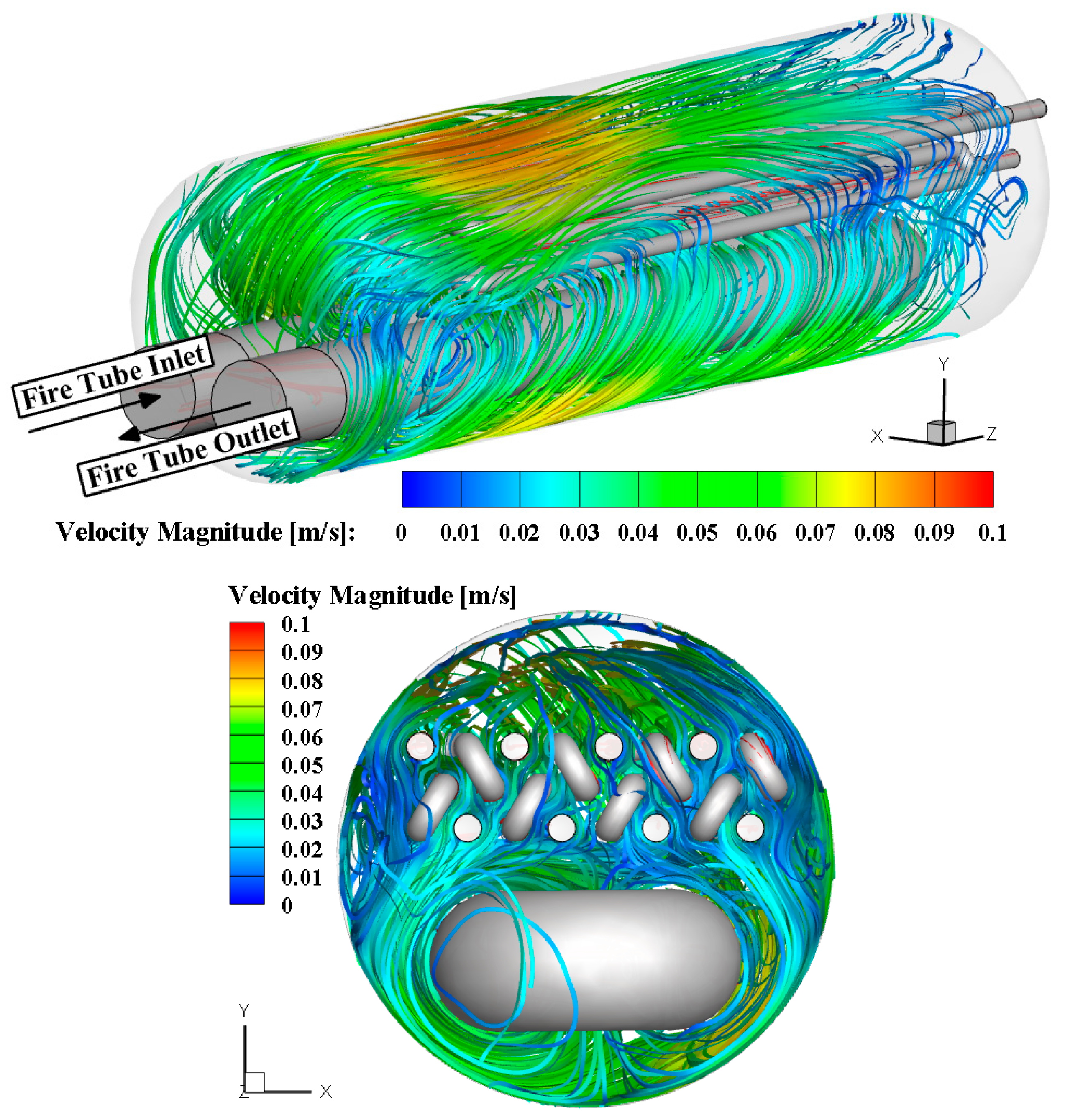
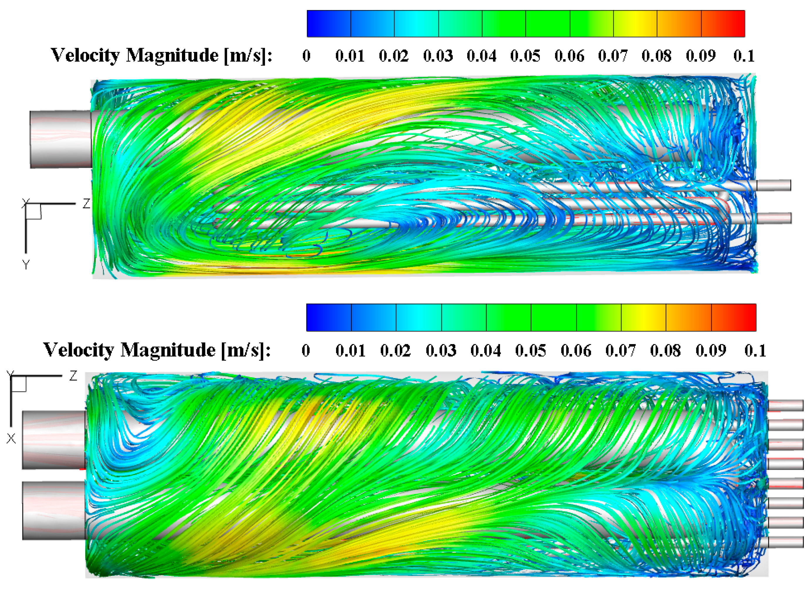
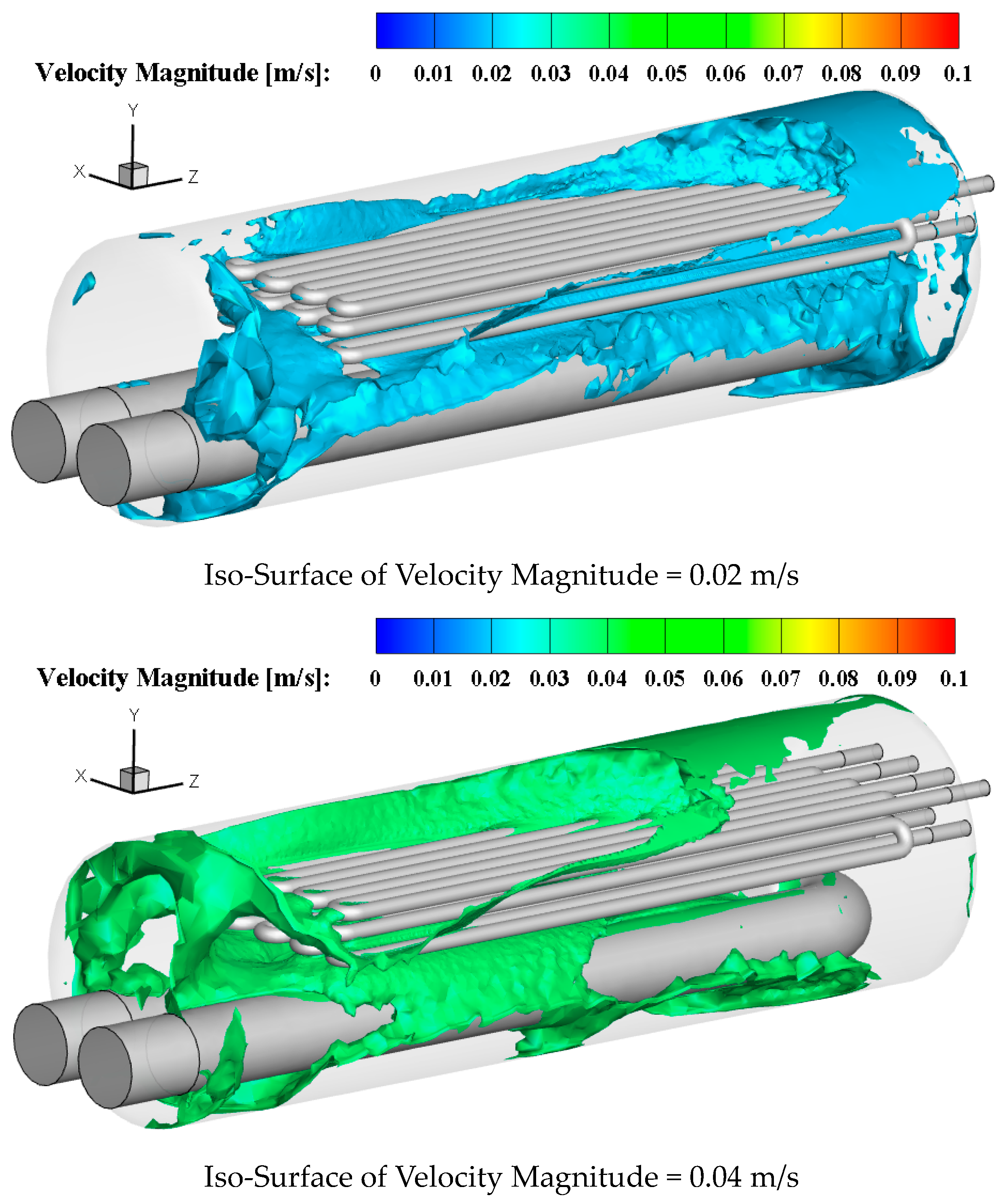
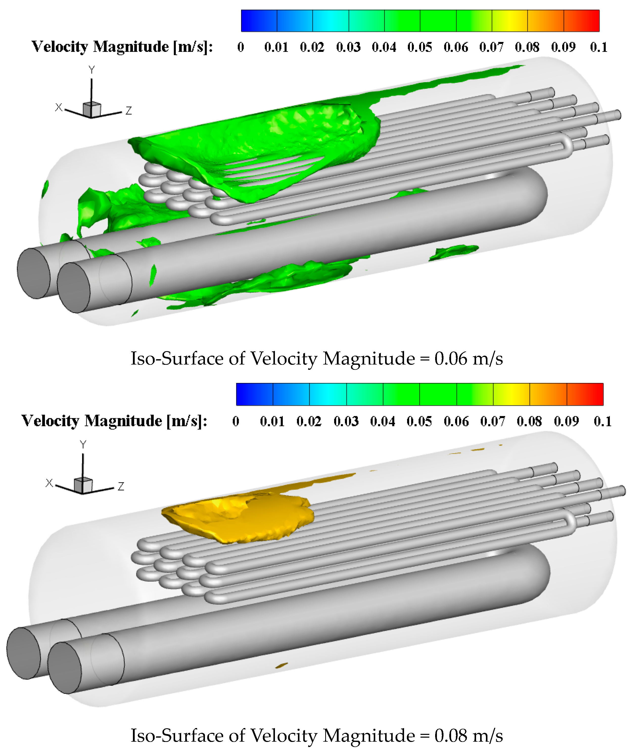
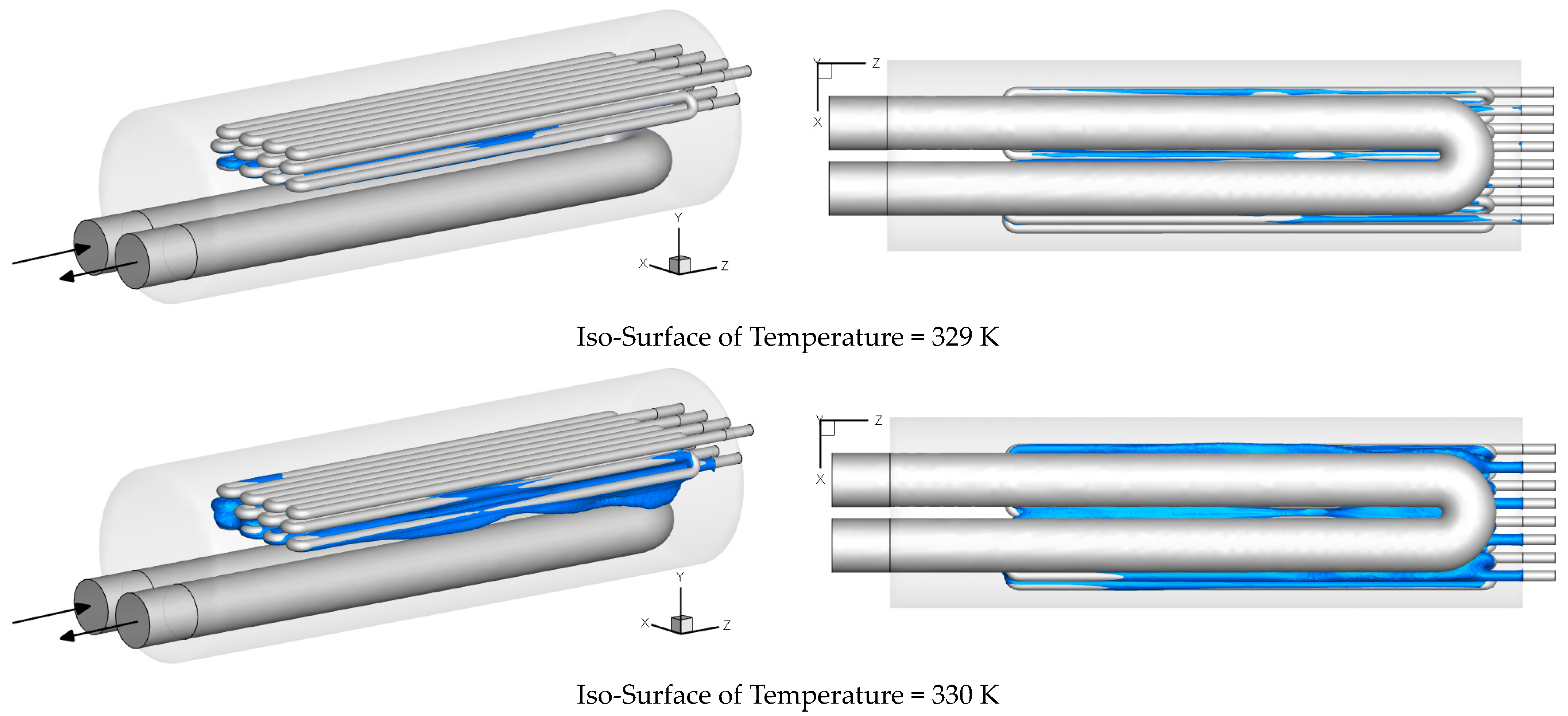
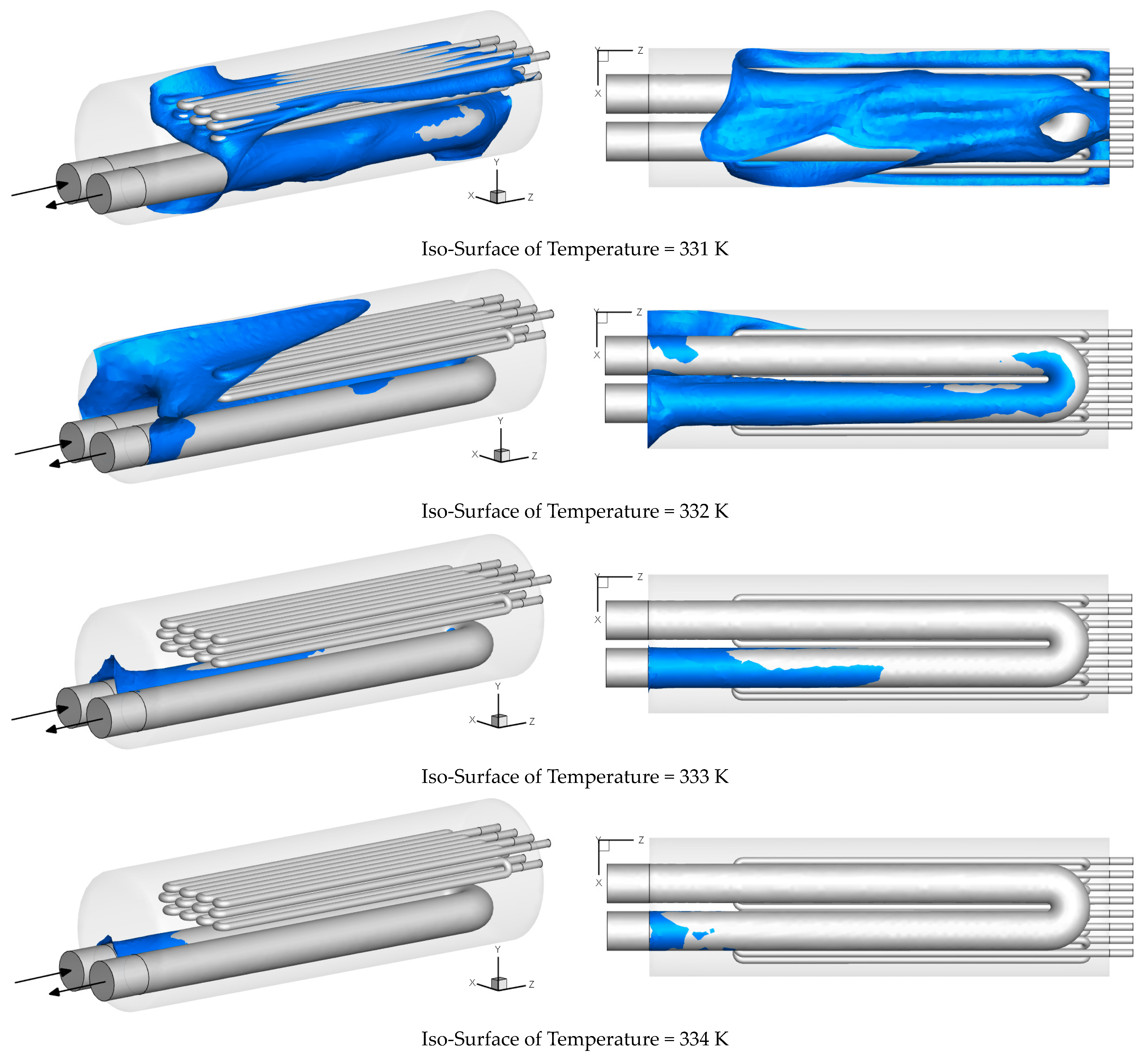
3.2. Investigating the Performance of the Gas Heater at 120,000 SCMH

Considering that very little work has been conducted in the field of gas heaters, this section first presents and then discusses one of the operating modes as an example of performance and modeling results. The modeling results for a full load are shown here. As mentioned earlier, in the modeling process, the inlet temperature of the gas was 10 degrees and the temperature of the combustion gases was 800 K. As the combustion exhaust gases entered the fire tube, heat exchange occurred across the surface of the tube with the water in the tank, resulting in a temperature drop in the tube. Figure 5 shows the temperature distribution of the liquid on a disk (Y direction) inside the fire tube. As can be seen, the temperature of the combustion exhaust gas dropped from 800 K to about 400 K.
The temperature difference inside the fire tube (Figure 6) resulted in a non-uniform heat flow on the surface of the fire tube. Figure 6 shows the distribution of the heat flux on the tube wall. As can be seen, the heat flux was greater at the inlet due to the higher temperature, and as the fluid approached the outlet and the temperature of the fluid decreased, the heat flux decreased. It is also clear that the assumption of a constant heat flux was not correct for the modeling of the fluid flow and heat transfer process in a fire tube. Negative values in Figure 6 indicate a loss of energy. The average value of the heat flux at the surface of the fire tube at full load was 27,000 W/m2.
The temperature difference between the cold source (methane cold gas coils) and the hot source (fire tube) and this uneven flux distribution led to asymmetric natural convection currents. The temperature and velocity distributions for three plates placed 2 m apart are shown (see Figure 7).
Figure 8 shows the temperature distribution across three slices (Figure 7). As can be seen, there was a significant temperature difference between the two paths of the fire tube, which created a buoyancy force and a different flow field. This temperature difference increased in the direction of the inlet and outlet plates, with the temperature difference on disc 3 reaching about 300 K.
Figure 9 shows the velocity distribution across the same discs but without the fire tube to better represent the true value of the fluid velocity. As predicted, the natural convection velocity that occurred near the inlet and outlet of the combustion exhaust was higher, reaching about 0.1 m/s, but in the discs farther from the inlet and outlet of the fire tube, the velocity difference was lower due to the smaller temperature difference.
Figure 10 shows the temperature distribution across the coil wall. As mentioned earlier, the heater under consideration consists of four coils. As can be seen, the lower tubes were colder due to the cold gas flowing in from below and were gradually heated by the flow of liquid through the hot water bath.
The heat flow through the coil wall is shown in Figure 11. As can be seen, the amount of heat absorbed by the coil varied along its length, and the assumption of a uniform heat flux as made in previous work was not a correct assumption. The average amount of heat absorbed by the coils was 13,700 W/m2.

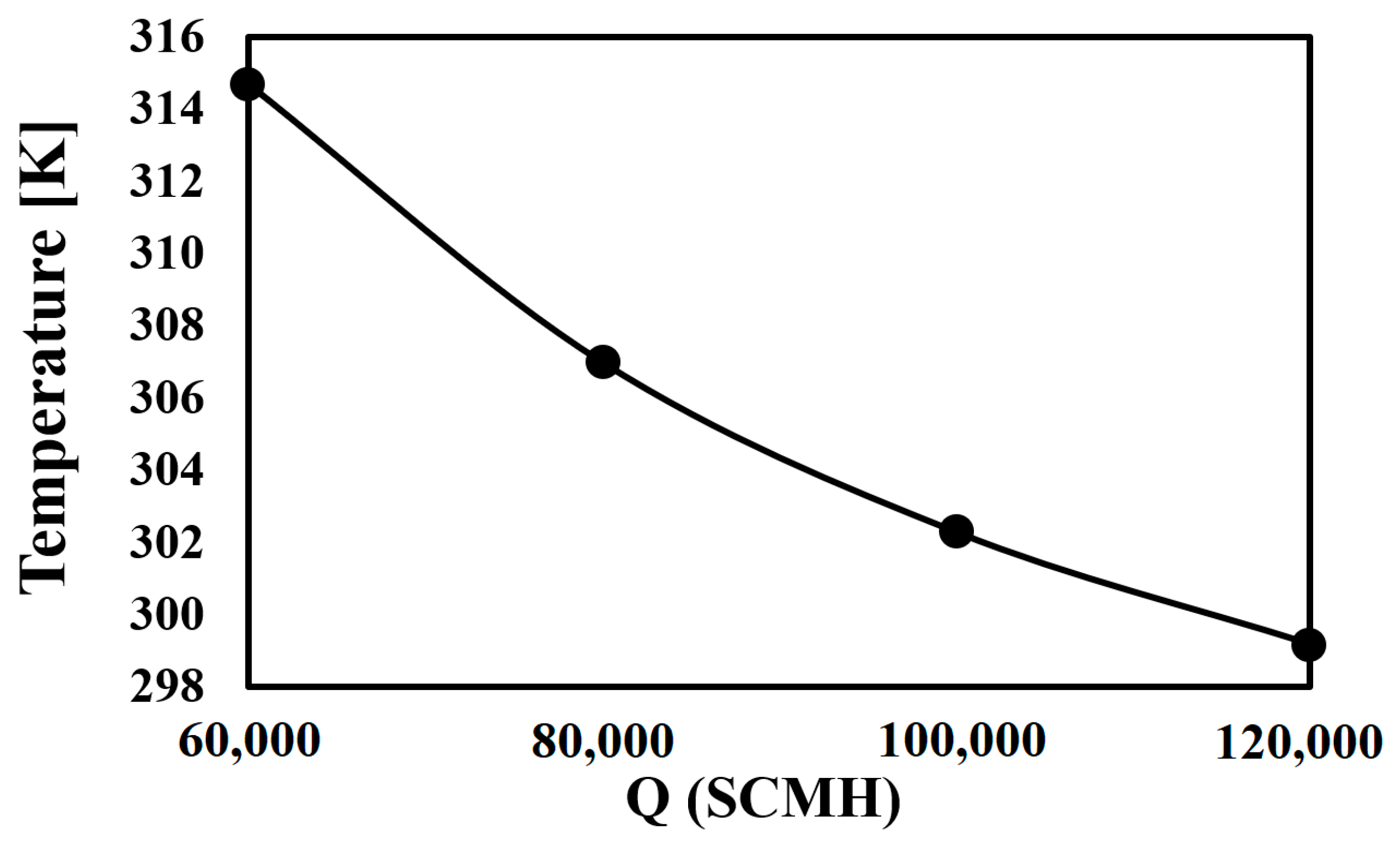
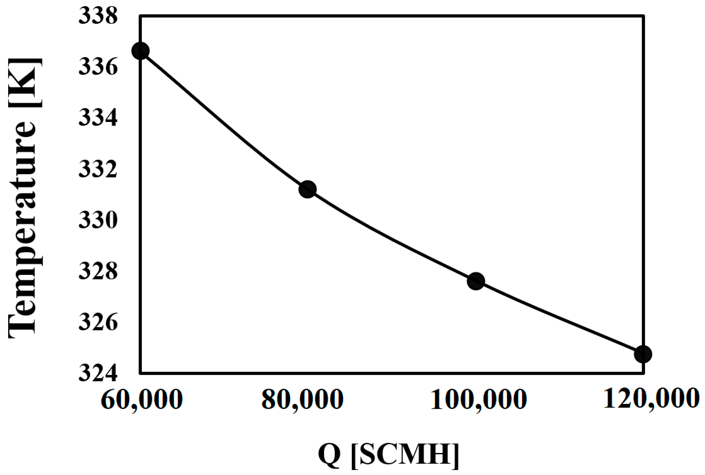
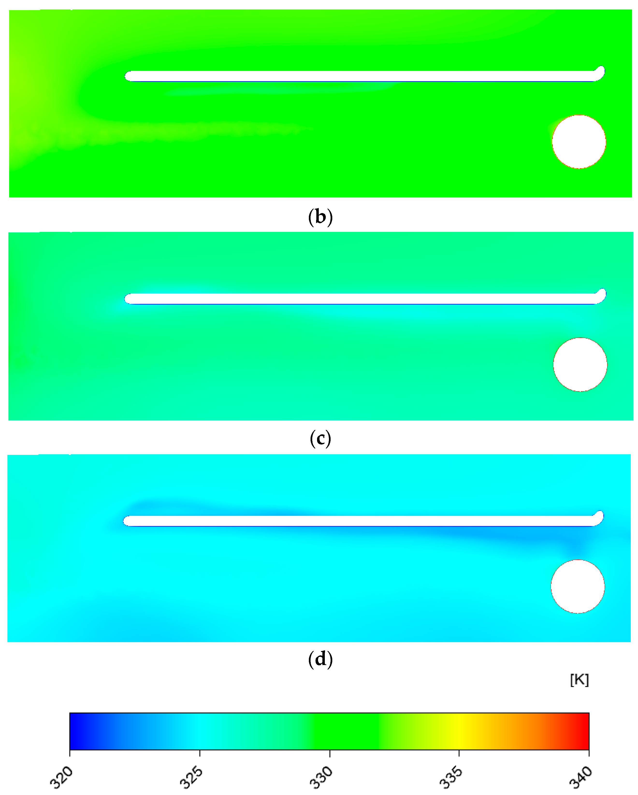
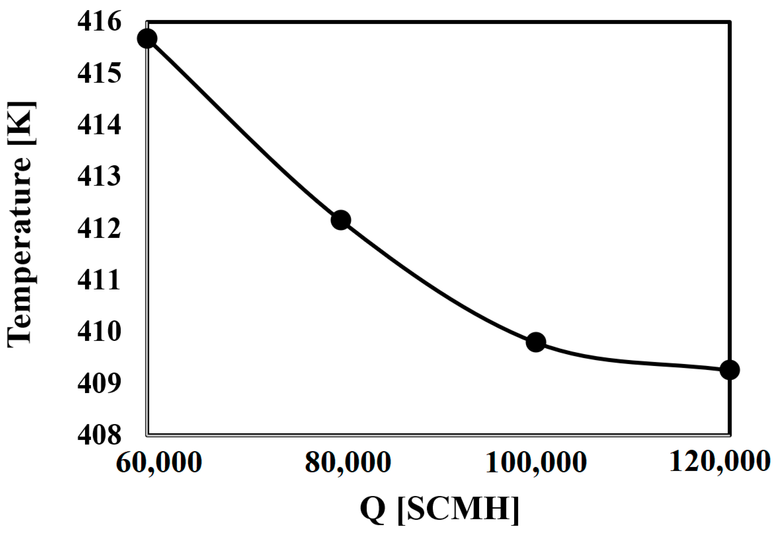
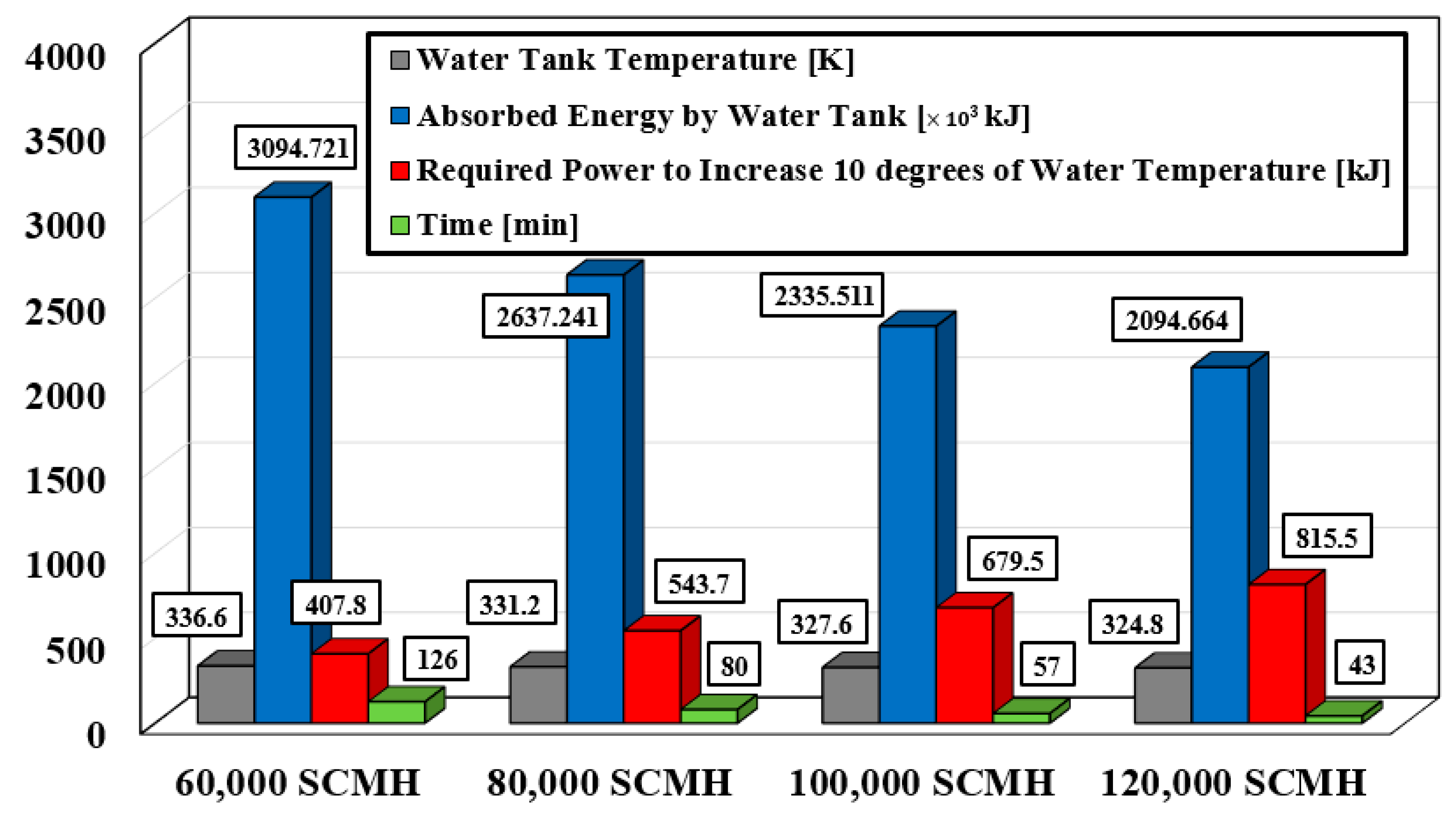
3.3. Investigating the Impact of Gas Mass Flow Rate

In this section, the thermal performance of the heater is presented at different gas mass flows, namely 60,000, 80,000, 100,000, and 120,000 SCHM (or 16.67, 22.22, 27.78, and 33.33 m3/s). The parameters studied in this section include the outlet temperature of the coil and the fire tube.
Figure 12 shows the exit temperature of the coil at different gas mass flows. As can be seen, the outlet temperature of the coil decreased as the gas mass flow rate increased, which was obviously due to the increase in the volume of liquid entering the heater. According to the numerical modeling results, the exit temperature decreased from about 315 K to 299 K with an increase from 60,000 (16.67 m3/s) to 120,000 (33.33 m3/s) SCHM (100% increase).
Figure 13 shows the average temperature of the hot water (on the shell side) as a function of the gas mass flow rate. As can be seen, the average temperature of the jacket liquid decreased when the gas mass flow rate at the coil was increased. According to the modeling results, when the gas inlet flow rate was 60,000 SCMH (16.67 m3/s), the average temperature of the hot water was 337 K, and with the increase in the mass flow rate to 120,000 SCMH (33.33 m3/s), the average temperature of the hot water decreased to 325 K. The temperature contours on a slice (X = 0) at different mass flow rates are shown in Figure 14. As can be seen, the water temperature inside the shell dropped significantly when the flow rate was increased.
The exit temperature of the fire tube is shown in Figure 15. As can be seen, as the mass flow rate of the coil increased, the exit temperature of the fire tube also decreased, so as the flow rate increased from 60,000 (16.67 m3/s) to 120,000 SCMH (33.33 m3/s), the exit temperature of the fire tube increased from about 416 to 409 K.
To better realize the natural convection process inside the water tank of the heater under consideration, the streamline inside the water tank considering the velocity magnitude is illustrated in Figure 16 from various perspectives. The impact of the buoyancy is clearly shown, and because of the density changes inside the tank, swirl flows were generated inside the tank, which can be seen in Figure 16.
The iso-surfaces with various values of velocity magnitude inside the water tank of the heater under consideration are illustrated in Figure 17. It can be seen that various values of velocity magnitude were reached in the water tank. The impact of buoyancy and density changes inside the water tank is also illustrated.
The iso-surfaces at various temperatures inside the water tank of the considered heater are illustrated in Figure 18. It can be concluded that most parts of the water tank had a range of temperature of 331–332 K. A lower temperature was observed around the gas tube and a higher temperature was observed around the fire tube.

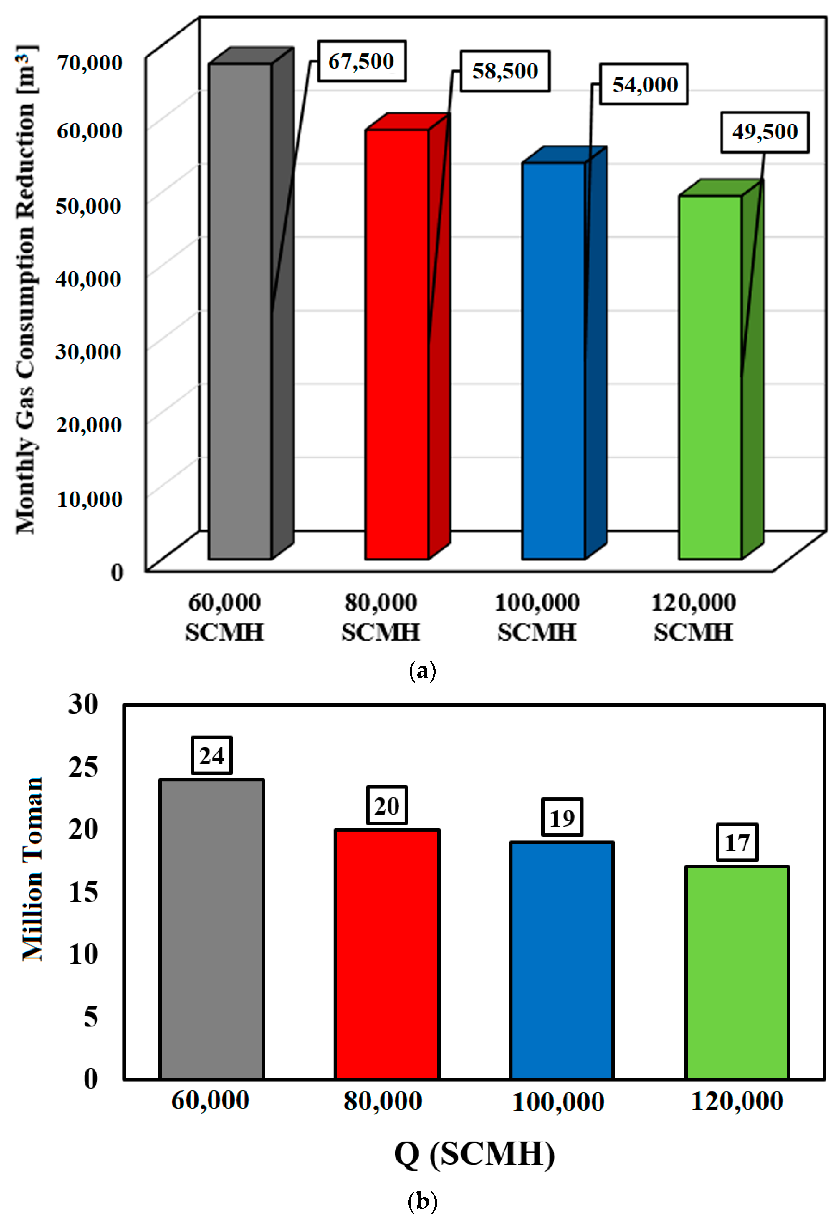
3.4. Investigating the Fuel Consumption Reduction Using the Considered Heater

Due to the high computational cost of this process, the amount of energy saved at different flow rates was calculated using simple calculations and is presented here. In other words, in these calculations, it is assumed that the temperature of the hot water bath leads to a minimum temperature of 20 degrees for the coil until a temperature drop of 300 K is reached. According to the calculations, 2 hours is needed at low flow rates and up to 43 min is needed at high flow rates. For example, the calculations for a flow rate of 60,000 SCMH are presented here. The energy available in the hot water bath is determined using below equation:
E = mC p ( T 2 T 1 )
where E is the energy in the hot water bath (kJ) when the burner is turned off, m is the fluid mass of the water inside the tank (kg), CP is the specific heat capacity of the water, and (T2 − T1) is the difference between the primary and secondary temperatures of the tank water.
The volume of the water tank is approximately 20 cubic meters and the average density of water is 1000 kg/m3. The initial temperature of the fluid, T1, is obtained according to numerical calculations employing ANSYS Fluent software and is the average temperature of the hot water bath. The secondary fluid temperature, T2, is assumed to be 300 K. Therefore, using the relationships and assumptions provided, the amount of energy stored in the hot water tank can be determined for different mass flow rates as we know the hot water bath temperature from numerical calculations. The amount of time it takes for the energy to be transferred to the fluid or, in other words, the time it takes for the temperature of the hot water bath to go from T1 to T2, can be calculated as follows:
E ˙ = m ˙ C p ( T 2 T 1 )
where E ˙ is coil (gas) power consumption, m ˙ is the mass flow rate of the gas inside the coil, CP is the heat capacity of the gas, and T1 and T2 are the initial and secondary temperatures of the gas, respectively. Finally, the time needed to transfer energy between the hot water bath and the coils, indicated as burner off time, is determined as follows:
t off = E E ˙
The burner off time needed to maintain a temperature of 20 degrees for the gas coil output is illustrated in Figure 19. It can be seen that as the gas mas flow rate increased from 60,000 SCMH to 120,000 SCMH (from 16.67 to 33.33 m3/s −100% growth), the burner off time declined by about 65.87%.
So far, the operating time has been calculated in the off-temperature mode. Now, in this continuation, it is necessary to calculate the time it takes from turning the burner on again to increase the temperature of the hot water bath to the previous value. After the burner is turned on, the energy from combustion is spent in two ways, increasing the temperature of the hot water bath and increasing the temperature of the coil gas:
t On = t Coil + t Water
where tCoil indicates the time required to heat the gas input to the heater, which, considering that the temperature of the output gas should not be less than 20 degrees, is continuously being heated and has no time delay. Additionally, tWater, which represents the time required to heat the water to the target temperature before the burner is turned off, is calculated as follows, considering the volume of the bath water and the difference between the desired temperature and the power of the burner:
q A = mC p ( T 2 T 1 ) t water
where q is the heat flux on the coil surface and A is the lateral area of the coil. The time elapsed from turning the burner on to meeting the target temperature for the hot water bath is presented in Figure 20. It is worth mentioning that the initial temperature of the water bath was kept constant at 300 K.
For a better understanding of the economic savings per month achieved for different flow rates of gas entering the station, the monthly reduction in gas consumption and the economic savings in tomans (official currency of Iran) are shown in Figure 21a,b, respectively. It can be seen that the maximum reduction in monthly gas consumption and the economic savings achieved using the proposed system were 67,500 m3 and IRR 25 million at a gas mass flow rate of 60,000 SCMH.

4. Conclusions

In this paper, the thermal performance of a gas heater of a pressure-reducing station at a pressure of 700 psi (4826.33 kPa) was numerically investigated. According to the numerical results, the thermal efficiency of the considered heater was about 70%, and at 100% full load and 50% full load, the gas temperature increased to 16.5 and 31 degrees, respectively. According to the studies performed, at a pressure of 700 psi (4826.33 kPa), the regulator causes a temperature drop of about 5 degrees. To prevent the gas from freezing in the regulator, according to the current standard and the station’s instructions, the gas should leave the heater at a temperature of about 20 °C at different operating pressures and enter the regulator, before finally entering the trunk line at 15 °C. According to the modeling results, the outlet temperature at a pressure of 700 psi (4826.33 kPa) is higher than required at various flow rates from 60,000 (16.67 m3/s) to 120,000 SCMH (33.33 m3/s), and by installing a regulator on the burner, gas consumption can be reduced.
As a continuation of the present work, we could focus on the type of fluid employed inside the heater tank and investigate the impact of using nanofluids with different types of nanoparticles and various volume concentrations instead of pure water on the thermal performance of the heater under consideration. Moreover, we suggest utilizing passive (no need for external force) heat transfer enhancement methods to improve the heat transfer rate in the heater under consideration, such as the use of corrugate pipes or extended surfaces (fins) with various geometries for the fire tube or natural gas pipes of the considered heater.

Author Contributions

Conceptualization, H.K.M. and S.S.M.A.; methodology, H.K.M. and S.S.M.A.; software, H.K.M.; validation, S.S.M.A., M.S.P. and M.A.; formal analysis, S.S.M.A. and M.S.P.; investigation, M.A.; resources, M.S.P.; data curation, M.S.P. and M.A.; writing—original draft preparation, H.K.M. and S.S.M.A.; writing—review and editing, M.S.P. and S.S.M.A.; visualization, M.A.; project administration, S.S.M.A. All authors have read and agreed to the published version of the manuscript.

Funding

This research received no external funding.

Data Availability Statement

The datasets generated during and/or analyzed during the current study are available from the corresponding author on reasonable request.

Conflicts of Interest

The authors declare no conflict of interest.

References

  1. Shokouhmand, H.; Rezaei Barmi, M.; Tavakoli, B. Gas Heater Availability Analysis and Consideration of Replacement Gas Heaters by Inline Heaters in the Pressure Reducing Stations of Natural Gas. In Proceedings of the ASME International Mechanical Engineering Congress and Exposition, Seattle, DC, USA, 11–15 November 2007; Volume 43025, pp. 1231–1240. [Google Scholar]
  2. Hedman, B.A. Waste Energy Recovery Opportunities for Interstate Natural Gas Pipelines; Interstate Natural Gas Association of America: Washington, DC, USA, 2008. [Google Scholar]
  3. Farzaneh-Gord, M.; Arabkoohsar, A.; Rezaei, M.; Deymi-Dashtebayaz, M.; Rahbari, H.R. Feasibility of employing solar energy in natural gas pressure drop stations. J. Energy Inst. 2011, 84, 165–173. [Google Scholar] [CrossRef]
  4. Clay, A.; Tansley, G.D. Exploration of a simple, low cost, micro gas turbine recuperator solution for a domestic combined heat and power unit. Appl. Therm. Eng. 2011, 31, 2676–2684. [Google Scholar] [CrossRef] [Green Version]
  5. Howard, C.; Oosthuizen, P.; Peppley, B. An investigation of the performance of a hybrid turboexpander-fuel cell system for power recovery at natural gas pressure reduction stations. Appl. Therm. Eng. 2011, 31, 2165–2170. [Google Scholar] [CrossRef] [Green Version]
  6. Andrei, I.; Valentin, T.; Cristina, T.; Niculae, T. Recovery of wasted mechanical energy from the reduction of natural gas pressure. Procedia Eng. 2014, 69, 986–990. [Google Scholar] [CrossRef] [Green Version]
  7. Ashouri, E.; Veysi, F.; Shojaeizadeh, E.; Asadi, M. The minimum gas temperature at the inlet of regulators in natural gas pressure reduction stations (CGS) for energy saving in water bath heaters. J. Nat. Gas Sci. Eng. 2014, 21, 230–240. [Google Scholar] [CrossRef]
  8. Farzaneh-Gord, M.; Ghezelbash, R.; Arabkoohsar, A.; Pilevari, L.; Machado, L.; Koury, R.N.N. Employing geothermal heat exchanger in natural gas pressure drop station in order to decrease fuel consumption. Energy 2015, 83, 164–176. [Google Scholar] [CrossRef]
  9. Ghezelbash, R.; Farzaneh-Gord, M.; Sadi, M. Performance assessment of vortex tube and vertical ground heat exchanger in reducing fuel consumption of conventional pressure drop stations. Appl. Therm. Eng. 2016, 102, 213–226. [Google Scholar] [CrossRef]
  10. Salari, S.; Goudarzi, K. Heat transfer enhancement and fuel consumption reduction in heaters of CGS gas stations. Case Stud. Therm. Eng. 2017, 10, 641–649. [Google Scholar] [CrossRef]
  11. Olfati, M.; Bahiraei, M.; Heidari, S.; Veysi, F. A comprehensive analysis of energy and exergy characteristics for a natural gas city gate station considering seasonal variations. Energy 2018, 155, 721–733. [Google Scholar] [CrossRef]
  12. Naderi, M.; Ahmadi, G.; Zarringhalam, M.; Akbari, O.; Khalili, E. Application of water reheating system for waste heat recovery in NG pressure reduction stations, with experimental verification. Energy 2018, 162, 1183–1192. [Google Scholar] [CrossRef]
  13. Rahmatpour, A.; Shaibani, M.J. Techno-economic assessment of gas pressure-based electricity generation (A case study of Iran). Energy Sources Part A Recovery Util. Environ. Eff. 2018, 40, 2236–2247. [Google Scholar] [CrossRef]
  14. Khosravi, M.; Arabkoohsar, A.; Alsagri, A.S.; Sheikholeslami, M. Improving thermal performance of water bath heaters in natural gas pressure drop stations. Appl. Therm. Eng. 2019, 159, 113829. [Google Scholar] [CrossRef]
  15. Noorollahi, Y.; Ghasemi, G.; Kowsary, F.; Roumi, S.; Jalilinasrabady, S. Modelling of heat supply for natural gas pressure reduction station using geothermal energy. Int. J. Sustain. Energy 2019, 38, 773–793. [Google Scholar] [CrossRef]
  16. Foo, K.; Liang, Y.Y.; Goh, P.S.; Fletcher, D.F. Computational fluid dynamics simulations of membrane gas separation: Overview, challenges and future perspectives. Chem. Eng. Res. Des. 2023, 191, 127–140. [Google Scholar] [CrossRef]
  17. Li, W.L.; Ouyang, Y.; Gao, X.Y.; Wang, C.Y.; Shao, L.; Xiang, Y. CFD analysis of gas–liquid flow characteristics in a microporous tube-in-tube microchannel reactor. Comput. Fluids 2018, 170, 13–23. [Google Scholar] [CrossRef]
  18. Siavash Amoli, B.; Mousavi Ajarostaghi, S.S.; Sedighi, K.; Aghajani Delavar, M. Evaporative pre-cooling of a condenser airflow: Investigation of nozzle cone angle, spray inclination angle and nozzle location. Energy Sources Part A Recovery Util. Environ. Eff. 2022, 44, 8040–8059. [Google Scholar] [CrossRef]
  19. Salhi, J.E.; Mousavi Ajarostaghi, S.S.; Zarrouk, T.; Saffari Pour, M.; Salhi, N.; Salhi, M. Turbulence and thermo-flow behavior of air in a rectangular channel with partially inclined baffles. Energy Sci. Eng. 2022, 10, 3540–3558. [Google Scholar] [CrossRef]
  20. Mohammadi, S.; Mousavi Ajarostaghi, S.S.; Pourfallah, M. The latent heat recovery from boiler exhaust flue gas using shell and corrugated tube heat exchanger: A numerical study. Heat Transfer 2020, 49, 3797–3815. [Google Scholar] [CrossRef]
  21. Nouri Kadijani, O.; Kazemi Moghadam, H.; Mousavi Ajarostaghi, S.S.; Asadi, A.; Saffari Pour, M. Hydrothermal performance of humid air flow in a rectangular solar air heater equipped with V-shaped ribs. Energy Sci. Eng. 2022, 10, 2276–2289. [Google Scholar] [CrossRef]
  22. Masoumpour-Samakoush, M.; Miansari, M.; Ajarostaghi, S.S.M.; Arıcı, M. Impact of innovative fin combination of triangular and rectangular fins on melting process of phase change material in a cavity. J. Energy Storage 2022, 45, 103545. [Google Scholar] [CrossRef]
  23. Pakzad, K.; Mousavi Ajarostaghi, S.S.; Sedighi, K. Numerical simulation of solidification process in an ice-on-coil ice storage system with serpentine tubes. SN Appl. Sci. 2019, 1, 1–12. [Google Scholar] [CrossRef] [Green Version]
  24. Riahi, M.; Yazdirad, B.; Jadidi, M.; Berenjkar, F.; Khoshnevisan, S.; Jamali, M.; Safary, M. Optimization of combustion Efficiency in indirect water bath heaters of Ardabil city gate stations. In Proceedings of the Seventh Mediterranean Combustion Symposium (MCS-7), Cagliari, Italy, 11–15 September 2011; pp. 11–15. [Google Scholar]
  25. Naderi, M.; Zargar, G.; Khalili, E. A numerical study on using air cooler heat exchanger for low grade energy recovery from exhaust flue gas in natural gas pressure reduction stations. Iran. J. Oil Gas Sci. Technol. 2018, 7, 93–109. [Google Scholar]
Figure 1. The 3D and 2D schematics of the studied heater.
Water 15 01469 g001
Figure 2. Contour of y+ distribution on the surface of the tube.
Water 15 01469 g002
Figure 3. The thermophysical properties of the exhaust gas flow in the fire tube as a function of gas temperature: (a) density, (b) viscosity, (c) heat capacity, and (d) thermal conductivity [25].
Water 15 01469 g003
Figure 4. Various views of the generated grid for the heater under study: (a) shell, (b) fire tube and gas tubes, (c) close-up of gas tube, and (d) different view of gas tubes.
Water 15 01469 g004aWater 15 01469 g004b
Figure 5. Temperature distribution across a slice (Y direction) inside the fire tube.
Water 15 01469 g005
Figure 6. Heat flux distribution across the fire tube wall.
Water 15 01469 g006
Figure 7. The position of the various slices (three slices) for presentation of the contours.
Water 15 01469 g007
Figure 8. The distribution of temperature in the various slices inside the shell: (a) Slice 1, (b) Slice 2, and (c) Slice 3.
Water 15 01469 g008aWater 15 01469 g008b
Figure 9. The distribution of velocity magnitude in the various slices inside the shell: (a) Slice 1, (b) Slice 2, (c) and Slice 3.
Water 15 01469 g009aWater 15 01469 g009b
Figure 10. The distribution of temperature across the coil wall from various perspectives.
Water 15 01469 g010aWater 15 01469 g010b
Figure 11. A 3D representation of the distribution of heat flux across the coil wall.
Water 15 01469 g011
Figure 12. The variation in the coil outlet temperature against the inlet mass flow rate.
Water 15 01469 g012
Figure 13. The variation in the shell (water) temperature against the inlet mass flow rate.
Water 15 01469 g013
Figure 14. The temperature distribution across the middle (X = 0) at various inlet mass flow rates: (a) m ˙ = 60,000 SCMH (16.67 m3/s), (b) m ˙ = 80,000 SCMH (22.22 m3/s), (c) m ˙ = 100,000 SCMH (27.78 m3/s), and (d) m ˙ = 120,000 SCMH (33.33 m3/s).
Water 15 01469 g014aWater 15 01469 g014b
Figure 15. The variation in the fire tube outlet temperature against the inlet mass flow rate.
Water 15 01469 g015
Figure 16. The streamline with the contour of velocity magnitude inside the water tank of the heater under study.
Water 15 01469 g016aWater 15 01469 g016b
Figure 17. The iso-surfaces of velocity magnitude with various values inside the water tank of the heater under consideration.
Water 15 01469 g017aWater 15 01469 g017b
Figure 18. The iso-surfaces at various temperatures inside the water tank of the considered heater.
Water 15 01469 g018aWater 15 01469 g018b
Figure 19. The burner off time versus the gas mass flow rate needed to maintain a temperature of 20 degrees for the gas coil output.
Water 15 01469 g019
Figure 20. The burner operation time elapsed before turning it off, after restarting it, and the duration of the burner operation at various gas mass flow rates.
Water 15 01469 g020
Figure 21. (a) The monthly reduction in gas consumption, and (b) the economic savings at different gas mass flow rates in one month.
Water 15 01469 g021
Table 1. Volumetric fraction of natural gas composition [24].
NameChemical FormulaVolume Percentage
Gas AnalysisLower LimitHigher Limit
MethaneCH488.3328595
EthanC2H64.67229
PropaneC3H84.1370.53
IsobuteneC4H100.4840.20.3
Normal ButaneC4H100.4840.250.5
IsopentaneC5H120.1810.10.15
Normal PentaneC5H120.1810.060.1
Carbon DioxideCO20.6940.10.4
NitrogenN24.525.7
SulfideH2S0.849 ppm1.256.25
Heavy/compound-00.020.2
Table 2. The thermophysical properties of methane at T = 20 °C and P = 700 psi (4826.33 kPa) [25].
PropertyValue
Density (kg.m−3) ρ 34.76
Specific Heat Capacity (kJ/(kg.K))CP2.57
Dynamic Viscosity (Pa.s)μ11.96 × 10⁻⁶
Static Viscosity (m2/s)υ0.344 × 10−6
Table 3. Composition of combustion exhaust gases [24].
Fuel Flow Rate (m3/hr)Carbon Monoxide (ppm)Carbon Dioxide (ppm)Nitrogen Oxides (ppm)Oxygen (%)Stack Temperature at Input Gate (°C)Ambient Temperature (°C)Combustion Efficiency (%)
102814.142213.692748.473.35
1112845.632511.603149.776.55
1802027.92397.204129.776.54
1863018.14376.644079.777.33
1921597.52337.734279.574.56
2041118.41426.164371.176.31
228448.36476.254550.875.11
252328.89575.314889.874.61
Table 4. The results of the mesh-independent analysis.
NumberGrid CellThe Outlet Temperature of the Methane (K)Error (%)
13,708,213313.20.45
24,777,825314.680.022
36,210,401314.61-
Table 5. The results of the Validation analysis.
NumberMass Flow Rate (SCMH (m3/s))Experimental Heater Outlet Temperature (°C)Numerical Heater Outlet Temperature (°C)Error (%)
180,000 (22.22)34.533.851.88
2100,000 (27.78)30.129.153.15
3120,000 (33.33)2726.053.52
Disclaimer/Publisher’s Note: The statements, opinions and data contained in all publications are solely those of the individual author(s) and contributor(s) and not of MDPI and/or the editor(s). MDPI and/or the editor(s) disclaim responsibility for any injury to people or property resulting from any ideas, methods, instructions or products referred to in the content.

