
Data Modeling of Sewage Treatment Plant Based on Long Short-Term Memory with Multilayer Perceptron Network
by
 , , ,
, , ,
Zhengxi Wei
1,2,
Ning Wu
2,*,
Qingchuan Zou
3,*,
Huanxin Zou
3,
Liucun Zhu
2,*,
Jinzhan Wei
4 and
Hong Huang
5 1
School of Computer, Electronics and Information, Guangxi University, 100 Daxue Road, Nanning 530004, China
2
Key Laboratory of Beibu Gulf Offshore Engineering Equipment and Technology, Beibu Gulf University, Qinzhou 535000, China
3
Guangxi Guohong Zhihong Environmental Technology Group Co., Ltd., Guigang 537100, China
4
School of Artificial Intelligence, Guilin University of Aerospace Technology, 2 Jinji Road, Guilin 541004, China
5
Nanning Sixun Electronics Technology Co., Ltd., Nanning 530007, China
*
Authors to whom correspondence should be addressed.
Water 2023, 15(8), 1472; https://doi.org/10.3390/w15081472
Submission received: 21 January 2023
/
Revised: 31 March 2023
/
Accepted: 3 April 2023
/
Published: 10 April 2023
(This article belongs to the Special Issue Advanced Machine Learning Techniques for Water)
Abstract
:As wastewater treatment usually involves complicated biochemical reactions, leading to strong coupling correlation and nonlinearity in water quality parameters, it is difficult to analyze and optimize the control of the wastewater treatment plant (WWTP) with traditional mathematical models. This research focuses on how deep learning techniques can be used to model the data from a specific WWTP so as to optimize the required energy consumption. In the operation of a wastewater treatment plant, various sensors are used to record the treatment process data; these data are used to train deep neural networks (DNNs). A long short-term memory with multilayer perceptron network (LMPNet) model is proposed to model the water quality parameters and site control parameters, such as COD, pH, NH3-N, et al., and the LMPNet model prediction error is then measured by criteria such as the MSE, MAE, and R2. The experimental results show that the LMPNet model demonstrates great accuracy in the modeling of the control of WWTPs. A life-long learning strategy is also developed for the LMPNet in order to adapt to the environment that may change over time. By developing performance evaluation metrics, the purification performance can be analyzed, and the prediction reference can be provided for the subsequent control optimization and energy saving plan.
1. Introduction
With the accelerating urbanization and industrialization and the growing population, the pressure on the usage of water resources has been increasing [1], and wastewater treatment technology as an effective means of water recycling consumes a large amount of electricity [2]. In recent years, wastewater treatment processes have been vigorously developed, and innovation-driven, next-generation wastewater treatment plants (WWTPs) have undergone continuous industrial structure optimization and technological upgrade. In order to reduce water pollution and maximize the water reuse rate to meet the challenges of sustainable water resource development, many countries have established a series of strict wastewater discharge standards, water reuse regulations, and wastewater treatment policies [3]. It is generally required that WWTPs must follow efficient biochemical reaction processes and have active bacterial purification units and precise energy-saving control strategies to improve the effectiveness of the wastewater treatment [4,5]. Due to the differences in the implementation of treatment specifications and the treatment processes used in each wastewater treatment plant, the operational data of each wastewater treatment plant vary. It is also worthwhile analyzing how these data are used in order to indirectly analyze the dynamic process of wastewater treatment [6,7].
Highly complicated reactions happen in the water treatment process, including biochemical reactions, fluid dynamics, sludge activity, deposition, biocatalysis, transport phenomena, and interactions between emerging micropollutants, and therefore, the variables representing the reactions are highly nonlinear and change dynamically. Consequently, it is difficult to analyze and predict the data of WWTPs for the purposes of energy saving and water safety [8,9]. Several studies have successfully demonstrated that the prediction of the future results of the wastewater treatment process can be accomplished through the analytical modeling of wastewater treatment plant data [9,10,11,12]. This research aims to predict the possible future water quality treatment results in order to optimize the wastewater treatment process.
The setup of the wastewater treatment plants depends on the location and the environment since the concentrations of the main pollutants in wastewater may vary and various types of sensor are required [13,14]. Rather than focusing on sensing, our research explores the application of deep learning techniques to model and analyze wastewater treatment data with better adaptability. In some cases, as municipal wastewater contains phosphorus and nitrogen compounds, direct discharge will accumulate and lead to eutrophication of water bodies, which can cause the excessive growth of plankton and attached algae and aquatic plants, resulting in considerable damage to lakes, reservoirs, rivers, and aquaculture environments [13]. Nutrient removal efficiency (RE) is an important indicator of the efficacy of these treatment plants, and continuous monitoring of the effluent treatment data is required to adjust the control strategies to keep the varying RE within a reasonable range while optimizing the power consumption. In most cases, energy consumption largely depends on the hydraulic retention time (HRT), the recycle ratio, the aeration rates, and the removal efficiency of ions [15]. The removal rate of total phosphorus (TP) and total nitrogen (TN) is also an important indicator of the effectiveness of the treatment process [14], and some studies have been conducted on the prediction of the removal rate of TP and TN [16]. Bioelectrochemical systems (BES) are an effective option for phosphorus removal and ammonia recovery due to the reduction in operating costs [17]. Combining model predictive control (MPC) with membrane bioreactor (MBR)-based hybrid systems is a promising solution for greater nutrient recovery from wastewater and improved economic efficiency of the treatment [18]. Recent studies have shown that the anaerobic-anoxic-oxic membrane bioreactor (A-A-O MBR) demonstrates a great performance in biological nutrient removal. Nitrosomonas, Nitrospira, Bacillaceae, and Rhodocyclaceae are generally regarded as the main nitrogen and phosphorus removal colonies, and in the anaerobic zone, the chemical oxygen demand (COD) can be converted to solution COD so that the quality of carbon source can be improved [19,20]. There have been examples showing that by modeling the data, the wastewater treatment process and management strategy can be accurately adjusted [6]. Benchmark simulation model no. 2 (BSM2) [21] or benchmark simulation model no. 1 (BSM1) [22] was also used as the baseline method for the modeling and analysis of wastewater treatment process due to its effectiveness [23].
The application of deep neural networks (DNNs) to the analysis and prediction of wastewater results has been a popular research topic in recent years due to the powerful nonlinear modeling and analysis capabilities [10]. It has been well documented that the application of deep learning model predictive control (DLMPC) with the support of artificial intelligence (AI) technology (data-driven modeling) is superior to the traditional models [24]. According to Mohammad et al., the modeling study of chlorophenols in wastewater using a multilayer artificial neural network with a genetic algorithm predicted better results than the several structures developed for the removal of the same chlorophenols using the reverse osmosis (RO) process [25]. In the analysis of wastewater treatment biofiltration membrane conditions, response surface methodology (RSM) and neural networks were used to optimize the operating parameters of membrane rotating biological contactors (MRBC) to reduce membrane contamination [26]. The relationship between COD and the trace elements can be accurately analyzed by modeling the chemical composition of the wastewater treatment process using DNNs. The WWTP can rely on data support from model analysis to develop more scientific and effective operations and management plans. The DNN is a useful tool for predicting wastewater treatment effectiveness and analyzing treatment plant performance, which can provide a technical guarantee for cost-effective and sustainable wastewater purification [9]. For a WWTP with an A-A-O MBR system, the effectiveness of water purification and the rate of nutrient removal can be related to a number of parameters, including total nitrogen (TN), total phosphorus (TP), dissolved oxygen (DO), COD, NH4-N, temperature, pH, total organic carbon (TOC), turbidity, etc. As wastewater treatment is a continuous process in time, the nature of the recorded data is that of a time series, and the long short-term memory (LSTM) model in a DNN can extract the time series feature in the data for more accurate analysis and prediction [16].
Traditional mathematical models find the explicit mapping relationships in parameters, and this is disadvantageous for the optimal adjustment of WWTP modeling according to the specific measured parameters [23]. In some small wastewater treatment plants, it is impossible to achieve a complete analysis due to the lack of expensive sensors [25]. Deep learning models can learn complex nonlinear mapping relationships between data from the training dataset recorded by the sensors, and it can be carried out flexibly according to the available measurement [23,27]. Previously, it was demonstrated that the radial basis function (RBF) neural network showed a level of performance in the critical control of wastewater treatment [28]; however, it was not suitable for the time sequence processing of dynamic treatment due to the disappearance of the gradient, while the LSTM model in the RNN series network can effectively solve these problems [11,16].
The operation of the WWTP requires a more intelligent water treatment model to optimize and enhance the stability of wastewater treatment performance. In this study, a deep learning technique is applied to model and analyze wastewater treatment process data for the optimization of the WWTP operation. The advantages of LSTM and MLP networks are combined to form a new model (LMPNet) with nonlinear time series analysis for the prediction of the wastewater treatment to solve the energy-saving problem in a WWTP located in the south of China.
The rest of the paper is organized as follows. Section 2 introduces the studied wastewater treatment plant, including a description of the wastewater treatment technology options used, how the relevant data were collected, and a preliminary analysis and collation of all the collected data. Section 3 discusses the selection of model hyperparameters and proposes the LMPNet model with lifelong learning and the method of performance evaluation. Section 4 demonstrates the training and testing experiments of the proposed model, and the experimental results are analyzed and discussed. Finally, the conclusions are given in Section 5.
2. Methodology
2.1. The Setup of the Studied WWTP
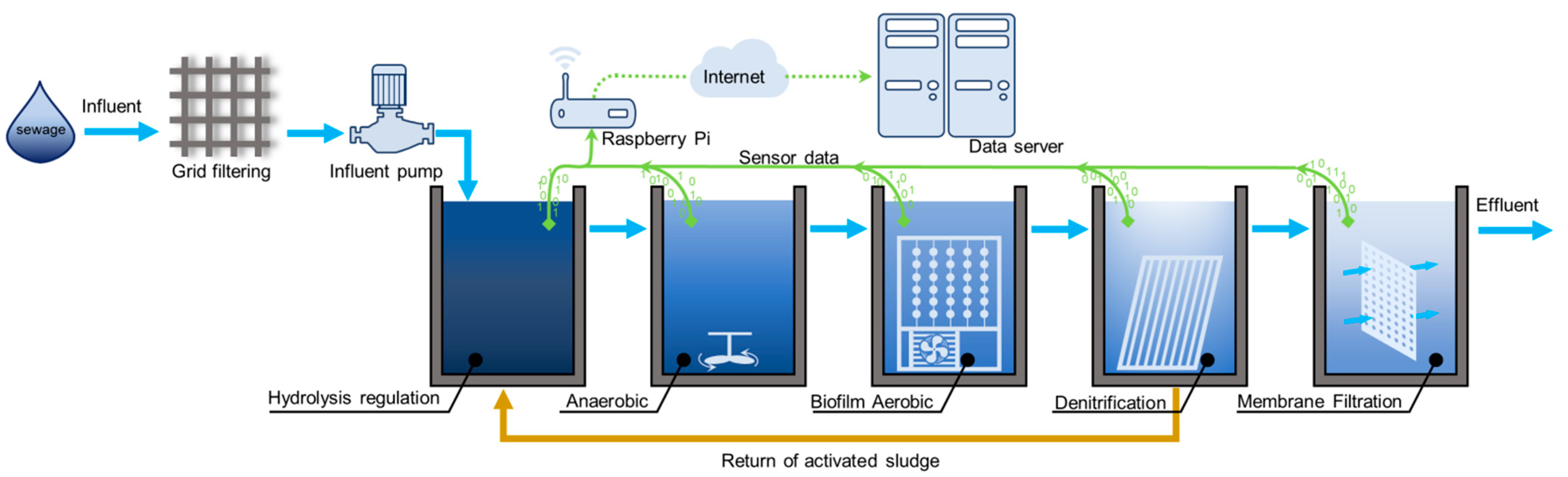
The DNN model developed in this research focuses on the WWTP setup based on dual-mode dynamic separation (DMDS) technology, as shown in Figure 1. The DMDS-based WWTP includes a hydrolysis conditioning tank, an anaerobic reaction tank, a biofilm aerobic reaction tank, a denitrification tank, and a fiber dynamic membrane filtration tank. After the preliminary filtration of wastewater through the grate, the wastewater is pumped into the hydrolysis tank by the lift pump for the preliminary water treatment, such as the precipitation of suspended impurities, hydrolysis of particulate matter, and pH adjustment. In the anaerobic tank, anaerobic bacteria are used to remove organic matter from the wastewater and to improve the biochemical properties of the wastewater for subsequent treatment. In the aerobic tank, the nutrients in the water are absorbed and transformed by the microorganisms through the biofilm, and the wastewater is de-nutrified accordingly. During this process, the fan continuously aerates the water to maintain the DO in a range that is conducive to the completion of active decomposition by aerobic microorganisms. The wastewater then flows into the inverse digester to further complete the denitrification process. Quartz sand is used as the membrane medium for denitrifying organisms and as a filtering structure for removing nitrate and suspended matter. A portion of the active sludge is allowed to flow back into the hydrolysis conditioning tank. In the final membrane filtration tank, dynamic biofilm interception and anti-pollution processing is carried out, and the microorganisms are quickly attached to form a piece of comprehensive biofilm by using a pre-coated biological agent-modified fiber mesh membrane as the support layer. After the processing in Figure 1, the water quality of the effluent flow is expected to meet the purification discharge standard in China.
As shown in Figure 1, the remote control center is a computer running a dedicated control program, which communicates remotely with matched end devices via the internet and acts as a data storage server for all the terminals. In the WWTP, sensor-recorded data can be monitored through the remote server to ensure that operations are carried out according to plan and strategy, thereby controlling the operating status of the pumps, fans, valves, and other equipment. The whole processing time can be adjusted by controlling the inlet water pump and valve. The adjustment of dissolved oxygen is completed by the aeration fan (F1, F2) in the biofilm aerobic pool with a DO sensor. As the DO value is critical for the biochemical reactions in wastewater treatment, if it is either too high or too low it will have an adverse effect on the water quality. Therefore, maintaining the stability of the DO of the water body through fan aeration is essential [28]. The input and output parameters are denoted with the subscripts in and out, respectively. The input COD, pH, and NH3-N are measured with sensors in the hydrolysis regulation pool, and the output parameters are measured in the membrane filtration pool. COD and NH3-N are also important indicators of the effectiveness of wastewater treatment [29]. The analog signals, such as the temperature, COD, pH, NH3-N, and drainage flow measured by each sensor, are collected and analyzed by an edge control system, Raspberry Pi. In each of the WWTPs there is a Raspberry Pi serving as an intermediate device for data communication and equipment control. The Raspberry Pi monitors the sensor data and receives control instructions from the remote server through the internet for the parameter adjustment of the equipment. The data of the water quality and operating status equipment are recorded minute by minute and are passed onto the DNN model in the remote server, Dell E31S, for analysis.
2.2. Dataset and Preprocessing
Due to the differences in the treatment process, the number and types of sensors used in different WWTPs vary considerably, and traditional mathematical modeling lacks the flexibility to handle the variation and the changes over time. In order to overcome these problems, an LMPNet model is proposed to adapt the variation and changes in data according to the different requirements, while keeping the backbone network intact so as to serve different WWTPs as a general and powerful tool [12].
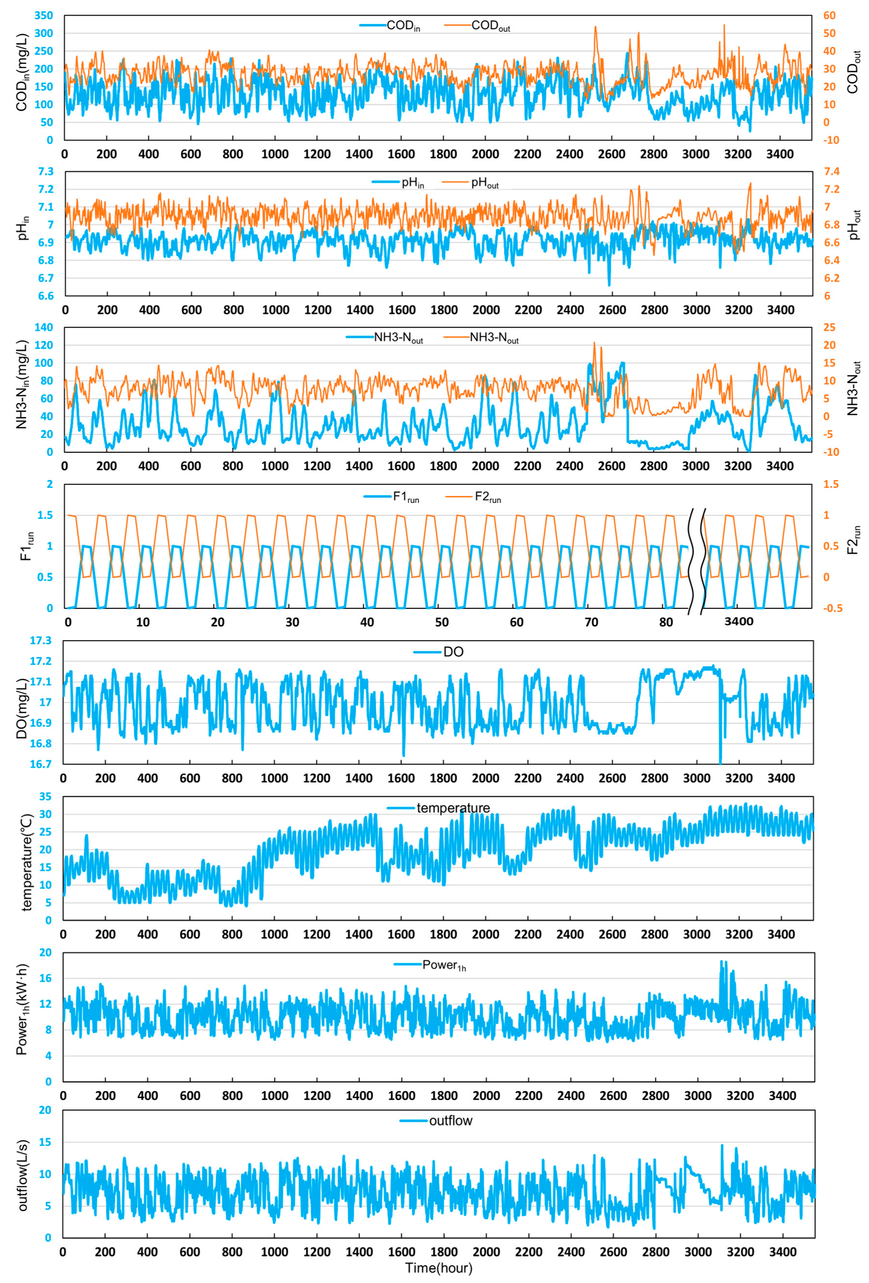
In the dataset preparation, we selected 12 water quality parameters with correlations for analysis, including CODin, pHin, NH3-Nin at the influent end, CODout, pHout, NH3-Nout at the effluent end, power consumption per hour Power1h, temperature, instantaneous flow rate at the effluent outflow, DO, fan 1 running status F1run, and fan 2 running status F2run. The data cleaning and pre-processing are essential to ensure the optimization of the LMPNet model, and therefore the recorded data were applied with the following steps before being used for the training and testing of the LMPNet:
- In the case of data missing due to failure in sensor communication, the previous value before the missing data will be used.
- In this WWTP setup, the sampling interval of the sensor is one minute, and in most of the time, the data value does not vary obviously within this interval. Therefore, in order to improve the learning efficiency, the mean value of the data within one hour is taken as the sampling point; in this way, there are 24 samples per day that will be recorded.
- For the fan operation status, the on status corresponds to the value 1, and the off status is 0.
In our experiment, a total of 3912 h of data was recorded from late February to late June of 2022 in a WWTP located in the south of China. Deep learning models generally require a large amount of training data to learn the underlying mapping patterns. Sufficient training data can help alleviate overfitting and improve the predictive performance of the model. Therefore, in this study a ratio of approximately 7:2:1 was adopted to divide the dataset, with the first 2842 samples as the training set, the next 710 samples as the validation set, and the last 360 samples as the test set. This method of dataset distribution helps to achieve a better performance and the generalization ability of the deep learning model, and it is also a widely accepted ratio in the field of machine learning. Figure 2 shows the value distribution of the original data for the 12 parameters, which will be further processed for the training and testing of the LMPNet. Table 1 shows the statistics of the 12 water quality parameters.
It can be seen from Table 1 that there is considerable difference in the ranges of value distribution due to the different scales of measurement. In order to ensure the consistency of the returned gradient of each parameter for the LMPNet and improve the model prediction accuracy of the small-dimensional input, the water quality parameters can be linearly standardized in order to improve the training convergence speed and prediction accuracy for small-scale parameters such as pHout and Power1h [7,30], such that,
where is the vector with the original values of the 12 parameters, and and are the mean and standard deviation vectors of the corresponding elements of , respectively. The output of Equation (1) will be the input of the first layer of the LMPNet model. The linear standardization maps the value distribution of the parameters to a standard normal distribution with zero mean and the variance of [0, 1], which preserves the distance information between samples and provides a more stable gradient descent during training.
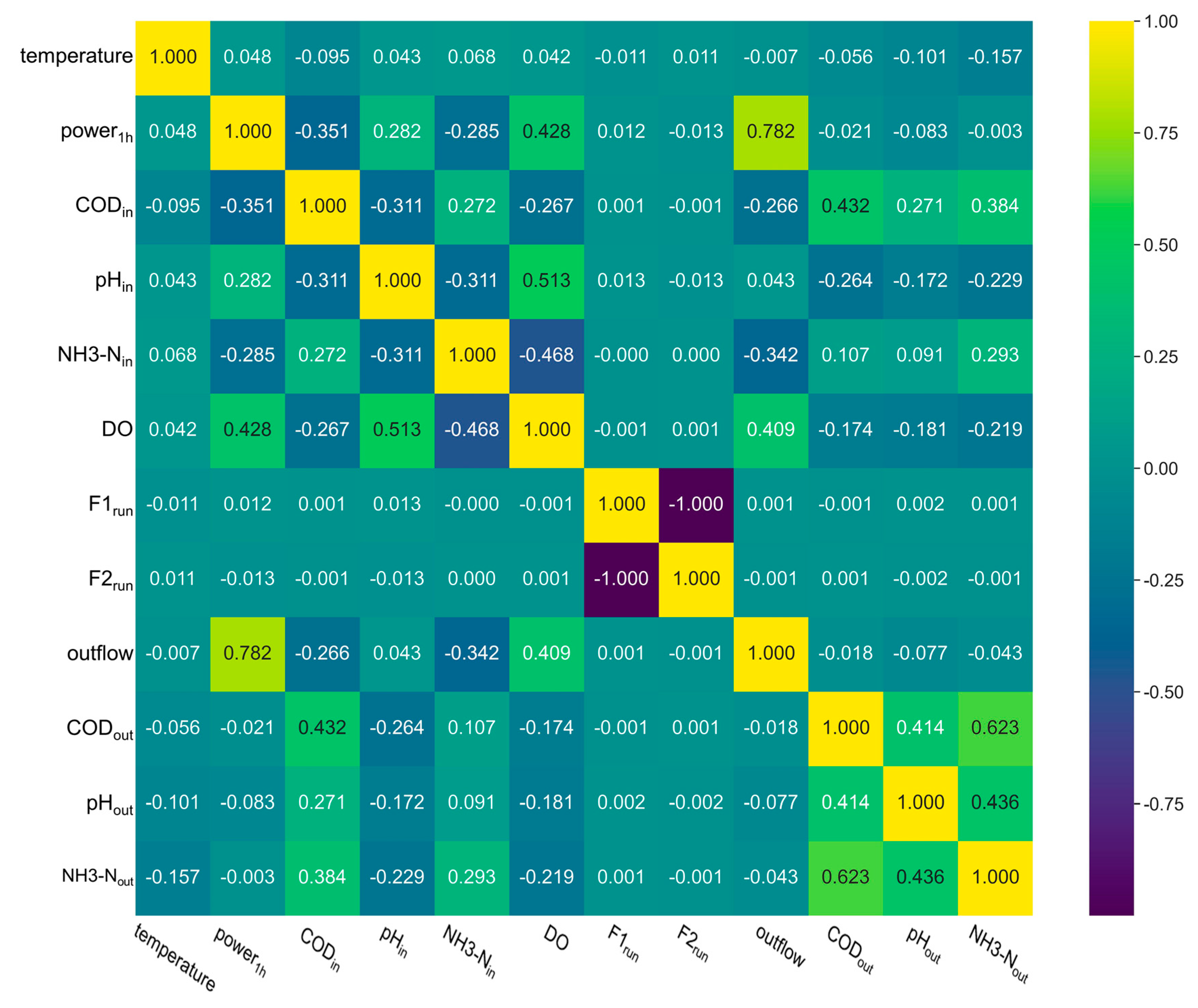
It is generally understood that there exists considerable inter-category correlation among the water quality parameters, which may affect the degree of convergence for the training of the LMPNet. Pearson’s correlation coefficient is an effective way to analyze the correlation among features based on covariance without considering the effect on the model analysis, and therefore, it was introduced to measure the correlation among the 12 water quality parameters [31]. The heat map in Figure 3 shows that there is a large positive correlation (0.623) between CODout and NH3-Nout, indicating that the COD content in this WWTP is related to the NH3-N content. F1run and F2run are in a regular alternating state of on and off, which presents the maximum negative correlation (−1), while the COD, NH3-N, and pH at the input and output are positively correlated (0.2~0.6) with each other. It can be seen that Power_1h shows the largest positive correlation (0.782) with the influent discharge outflow. The largest negative correlation (−0.468) is between the DO and NH3-N. Pearson’s correlation can only be used for the preliminary analysis of the intra-class correlation and the inter-class discriminability of the training set; however, there may be a very complex nonlinear correlation within the data which cannot be reflected.
3. The LMPNet Model
3.1. The Hyperparameters Selection
It is necessary to select the structure and the structural hyperparameters of the model according to the specific engineering problem. In this research, the structure and the structural hyperparameters were determined by carrying out experiments with many other networks to select the most suitable one. The hyperparameters of the LMPNet include structural and training hyperparameters which are essential for the prediction performance, such as the number of variables within the model and the size of the training set [32]. For the structural hyperparameters, if the LMPNet does not have enough variables and layers, the model’s nonlinear regression capability would not be sufficient for the representation of the samples, resulting in low prediction accuracy. If the LMPNet was too deep and densely connected, the computational complexity would be overloaded, leading to overfitting problems [16,33], and it would not be possible to deploy the model on edge devices, although the performance could be improved [34]. It is essential to choose the appropriate structural hyperparameters based on the task and computational budget, and in this study, a set of hyperparameters most suitable for this application was found by carrying out several experiments and analyses on the LMPNet structure. For the training set of the LMPNet, a set of suitable training hyperparameters was prepared through the training experiments, including the batch size, dropout rate, number of epochs, optimizer, learning rate, weight decay, train and validation set split ratio, and loss function [34]. Table 2 shows the training hyperparameters used in the LMPNet. The LSTM module was introduced to extract the temporal features between the data, which will be fed into a 4-layer fully connected layer for nonlinear modeling. The nonlinear activation function PReLU is used to ensure the gradient stability of the model during training. The dropout layer is in place to reduce the overfitting. The structural and training hyperparameters of our proposed LMPNet network were determined after several experimental analyses and the continuous optimization of the network structure based on specific engineering requirements. In order to ensure the consistency of the experimental analysis, the same hyperparameters were used in all experiments in this research.
3.2. The Structure of the LMPNet
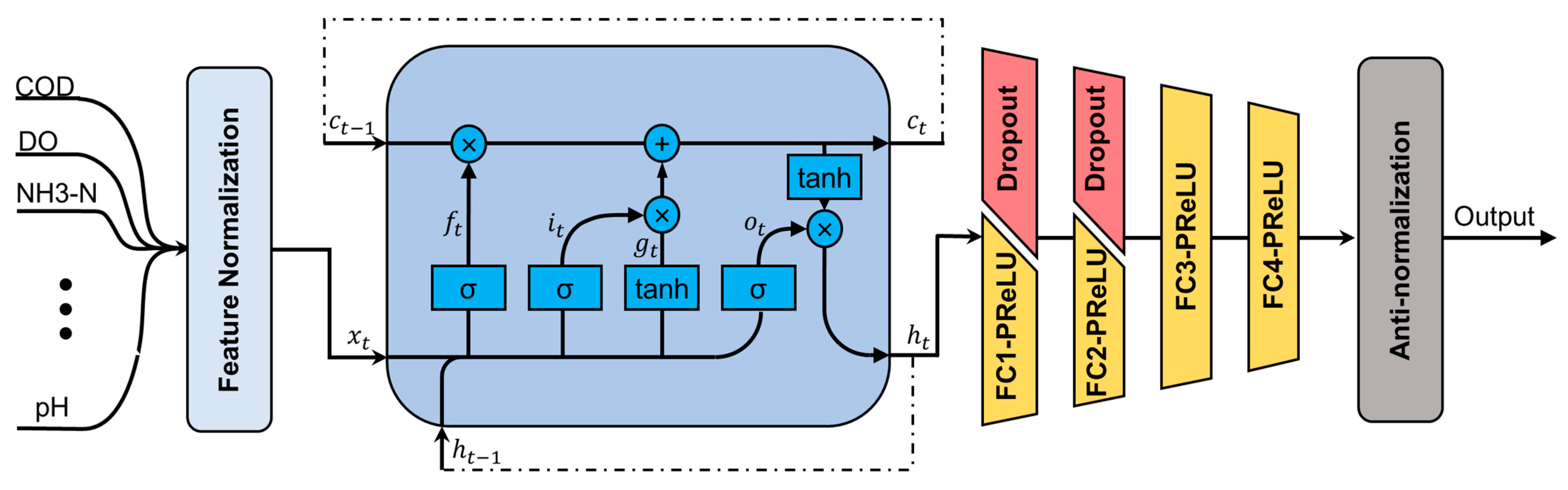
Figure 4 shows the network structure of the LMPNet model; it is coded based on the Pytorch deep learning framework.
In the LMPNet model, the input is a vector with 12 parameters of water quality, such as the COD, DO, NH3-N, etc., and the feature normalization layer carry out the standardization of to generate at time t. An LSTM network was designed to process ; it outputs the hidden state to an MLP network where a nonlinear mapping transformation is applied to . An anti-normalization layer is then followed for the data post-processing; it outputs the predicted water quality parameter vector of .
The nonlinear activation functions in the LMPNet model help to enable the nonlinear modeling capabilities, and in this model three different types of nonlinear functions were applied: the Sigmoid function, the hyperbolic-tangent function, and the PReLU function [35]; they are given, respectively, as,
where is the input vector and is a learnable parameter.
As one of the most popular networks for temporal feature classification, the LSTM can dynamically memorize the changes in data with a structure of feedback connection [36]. Considering that wastewater treatment is a dynamic and continuous process, the one-layer LSTM cell in the LMPNet extracts the temporal features from the input data xt, such that,
where is the input at time t, is the output and hidden state, and is the hidden state of the layer at time t − 1 or 0 at the initial state. and are the cell state at time t and t − 1, respectively, and the value at the initial cell state is also 0. , , , are the input gate, forget gate, cell gate, and output gate, respectively, and is the Hadamard product. The variables of W and b with a two-dimensional suffix are learnable weights and offset parameters, respectively.
In the MLP module of the LMPNet structure, there are four fully connected (FC) layers, for each of which a PReLU is used as the activation function. The numbers of neurons in the FC1 to FC4 layers are 128, 64, 32, and the number of water quality parameters, respectively. In order to reduce the overfitting effect, a dropout layer is used in both layer 1 and layer 2 so that each neuron in FC1 and FC2 has a 50% probability of deactivation during the training process. The output of the MLP is fed into the anti-normalization layer, which generates a denormalized output.
3.3. Performance Evaluation
The performance of the LMPNet was evaluated to ensure that the application was efficient and stable [37]. In this study, the metrics of the mean square error (MSE), the mean absolute error (MAE), and coefficient of determination (R2) were introduced to evaluate the prediction results of the LMPNet, such that,
where is the number of testing samples, and are the label vectors and model-predicted vectors, respectively, and is the mean vector of the true values. , and are vectors with three elements representing the MSE, MAE, and R2 values of the CODout, pHout, and NH3-Nout, respectively. The value ranges of Equations (12) and (13) are ∈ [0, +∞) and ∈ [0, 1], respectively. The smaller the MSE value, the closer the is to 1 and the better the prediction performance that is achieved [38].
3.4. Model Lifelong Learning
In the case that a DNN model was trained for the data collected from a specific WWTP, if the distribution of the parameters changed due to the change in environment, the purification equipment, or the treatment process, the nonlinear relationships within the parameters learned by the model may be outdated, and therefore, an update or relearn of the model is required. If a model cannot continuously optimize itself according to the change in environment, the prediction accuracy may decrease and eventually fail to function. This problem can be overcome by using a lifelong learning strategy (continuous learning or incremental learning) to maintain a high prediction accuracy of the model during applications [39].
In the operation of the WWTP in this research, all the data recorded from wastewater treatment were continuously collected by the remote servers for storage and nonstop training of the LMPNet model. In this lifelong learning strategy, the LMPNet model was trained incrementally every month based on the previous version, using the data collected in the previous 6 months. In this incremental training, the combined approaches of pre-training and fine-tuning were applied, and the LMPNet model was loaded with weight parameters containing historically learned status and then trained on a new training set for 10 epochs. This allowed the model to focus more on learning from new data while retaining previously learned knowledge. Through lifelong learning, the LMPNet model will continue to optimize itself to ensure high prediction accuracy even if the status of the WWTP or environment has changed.
4. Experimental Results and Discussion
4.1. Output Water Quality Prediction with LMPNet
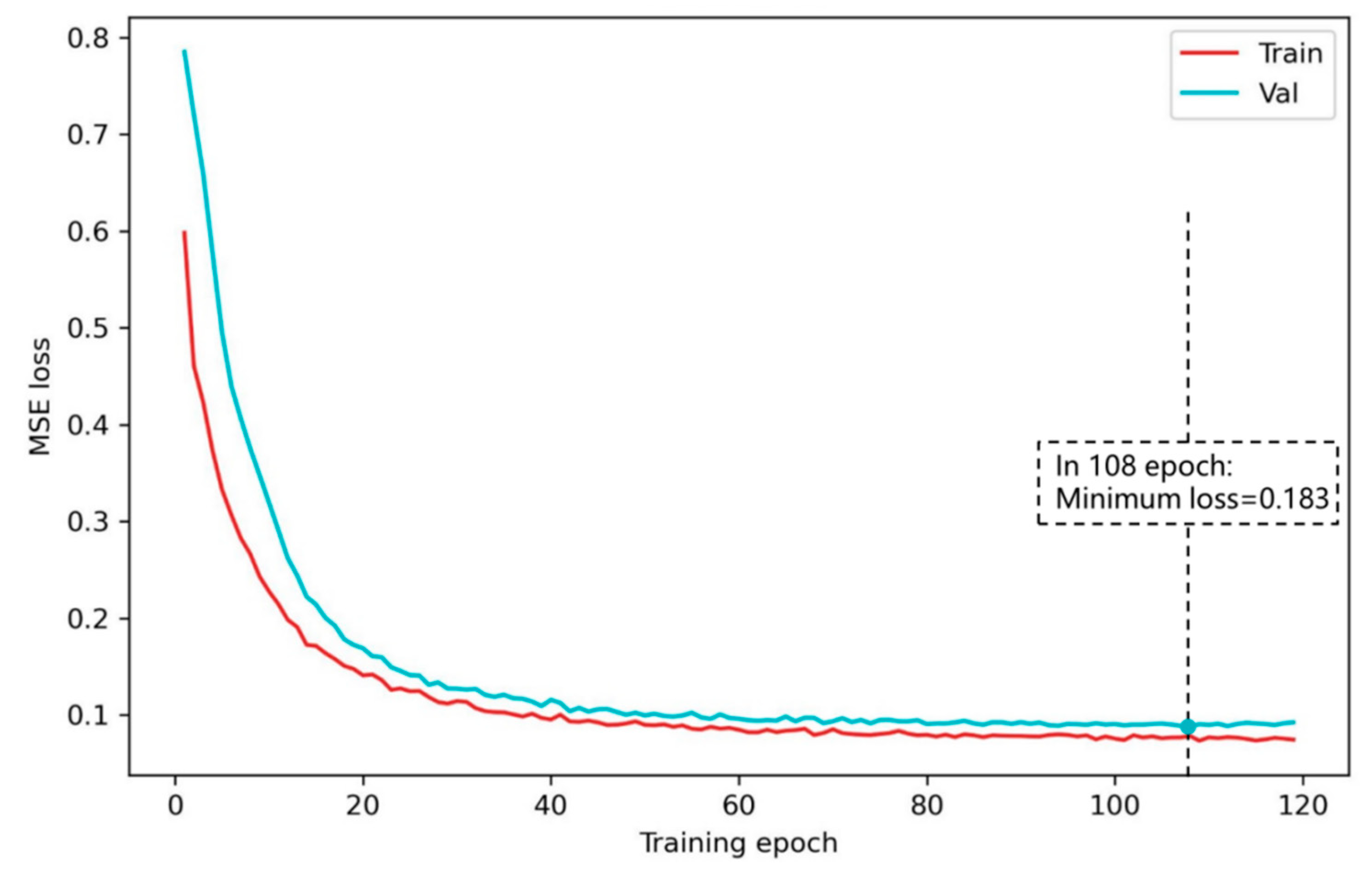
As wastewater treatment is a dynamic and continuous process, it will take some time to go through the five biochemical reaction tanks from purification to discharge, as shown in Figure 1. The processing time for the wastewater treatment generally varies dynamically within a certain range; however, the data prediction by the LMPNet will measure a fixed time span (Δt) and label it as one of the categories. After the preliminary analysis of the HRT, the LMPNet was applied to predict the COD, pH, and NH3-N parameters of the output water after a 9 h time span. The parameters of COD, pH, and NH3-N are important indicators of the quality of the wastewater purification. In the training of the LMPNet, the water quality data recorded from January to June 2022 was divided into 2840 training samples and 711 validation samples at the ratio of 8:2. Then, the 360 samples recorded in the following 15 days were used as test samples to analyze the model performance. The weights with the smallest validation loss were taken as the optimal weight solution for the implementation of the LMPNet. In the testing set, the optimal weights were used to test the performance of the LMPNet in order to more precisely reflect the consistency and generalization of the prediction accuracy of the LMPNet. In this training process, the Adam algorithm [40] was used as the optimizer and the learning rate was set to 0.0003. The regression loss function MSELoss was chosen as the objective function for the training, and a smaller loss value resulted in a more accurate prediction. In order to ensure data continuity, we did not use shuffle operations when loading data into the model. The specific model training configuration can be seen in Table 2. The decrease in the MSEloss value during the training process is shown in Figure 5.
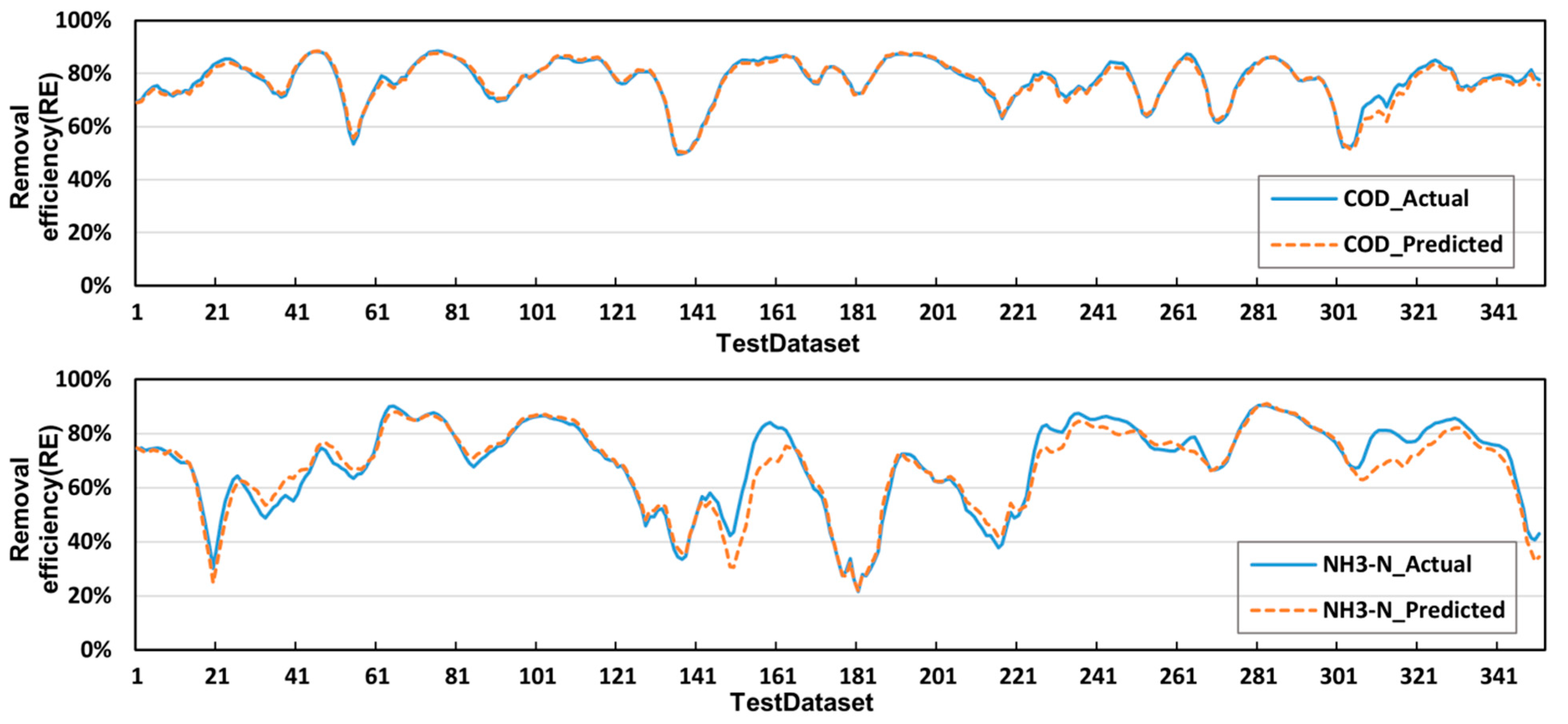
The prediction performance of the model was tested on the test set, and the predicted and the actual values are compared in Figure 6. It can be seen that the actual value curve is well approximated by the predicted value curve at the Δt of 9 h. From a quantitative perspective, the MSE and MAE values representing the prediction errors of the parameters of CODout, pHout, and NH3-Nout are [2.129, 0.006, 0.706] and [1.198, 0.054, 0.650], respectively, and the values of the three elements of R2 are [0.799, 0.490, 0.824]. The pH data remain in a small range of around 7, which makes it difficult for the model to learn the nonlinear mapping within the data, and it only learns to output a value very close to 7. The value range of CODout is the largest (20~34), and the maximum absolute error of prediction is only 2.45. The mean absolute percentage error (MAPE) of the model predictions for CODout, pHout and NH3-Nout are 4.6%, 0.8%, and 12.3%. It can be seen that the prediction accuracy of LMPNet meets the engineering requirements, and the prediction output of CODout, pHout, and NH3-Nout can effectively indicate a warning to the possible substandard of wastewater purification. The actual and predicted RE results are compared in Figure 7 to evaluate the efficiency of the proposed LMPNet model. The results showed that the curve fit of the RE is satisfactory due to the accurate prediction by LMPNet, which will be useful in the optimization of the automation and control of a WWTP.
4.2. The Ablation of the Input Water Quality Characteristics
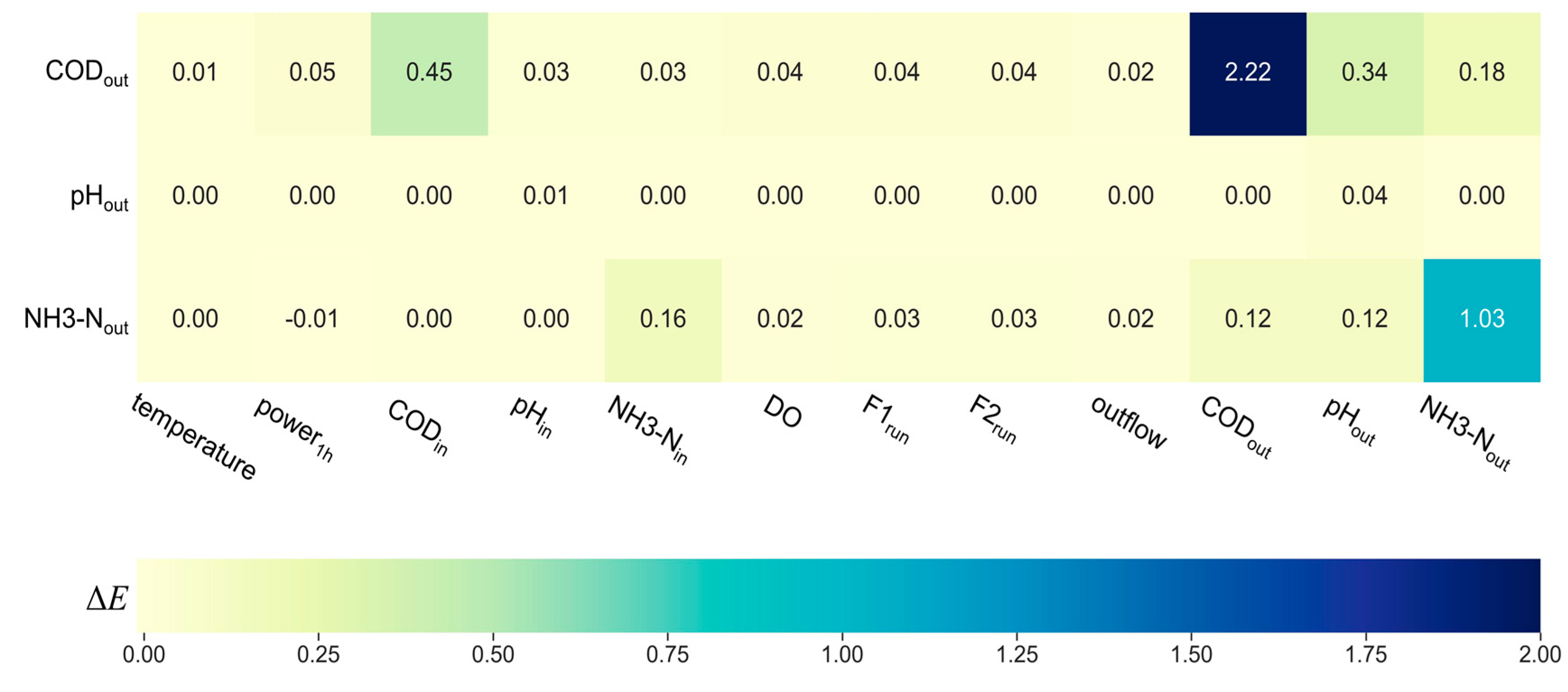
The correlation between the input and output water quality features differs from plant to plant; however, in the model prediction, a stronger correlation feature pair generally led to the decrease in the prediction accuracy if one of the parameters was absent or distorted in the input. For this reason, a feature ablation experiment was carried out to analyze the effect of each of the water quality features on the predicted output. Referring to the LMPNet prediction experiment in Section 4.1, the MAE vector [1.198, 0.054, 0.650] was regarded as the benchmark for the predicted CODout, pHout, and NH3-Nout values, defined as ; the absence or distortion of any one of the three parameters resulted in an increase in the MAE values. If the ith element of the input data was removed from the input vector, leaving xt only 11 elements in the same order, the resulting MAE value vector was denoted as , and its deviation from the is given as,
The metric of represents the importance of a corresponding water quality parameter in the input, and Figure 8 shows the values of for each of the 12 parameters in the input based on all the recorded data. Generally, there is an increase in the value when one of the input parameters is removed, and a bigger corresponds to a more important input parameter to the prediction of the output features. It can be seen from Figure 8 that each of the current output features of the LMPNet is mainly influenced by the corresponding pair of water quality features after one hour; these pairs include those of CODout and CODin, pHout and pHin, and NH3-Nout and NH3-Nin, respectively. The rest of the water quality features have very little influence on the three predicted elements when removed from the input. These results show the effectiveness of the LMPNet on the water quality prediction in a 9-hour time period because these water quality features are always within a relatively stable value range, and any fluctuation in an input parameter will result in an offset of the prediction for the corresponding output feature.
4.3. Influence of Different Time Delays on Prediction
The purpose of the experiments in this subsection was to analyze the prediction performance of the model at different time spans. Following the experiments in Section 4.1 to predict the parameters such as the CODout, pHout, and NH3-Nout with a delay of Δt = 9 h, this section tests the LMPNet with different time delays of Δt = 6, 8, 10, 12, 14, and 16 h, respectively. Table 3 shows the performance analysis metrics of the MAE and MSE between the predicted and true values of the model. The experimental results show that LMPNet can maintain a good prediction performance within a range of time spans. The variation in prediction accuracy is related to the HRT of the wastewater treatment process.
4.4. Energy Efficiency Analysis for Wastewater Purification
The energy efficiency of the wastewater treatment process can be analyzed and predicted based on the COD and NH3-N concentrations at the input and output, the purification volume, and the energy consumption. A synthesized purification factor R was defined to measure the amount of purification level between the input and output, as follows,
where and are the weighting factors to balance the difference between COD and NH3-N, and they are set to 0.1 and 0.4, respectively, based on experimental analysis. and are the COD concentrations of water at time t at the input and output, respectively. and are the NH3-N concentrations at time t at the input and output, respectively. The net water discharge at time t is defined as,
where is the instantaneous flow rate of the output water. The purification efficiency factor η at the hour of t is defined as the average ratio every four hours between the net water discharge volume weighted by the purification factor R over the power consumption per hour and is given as
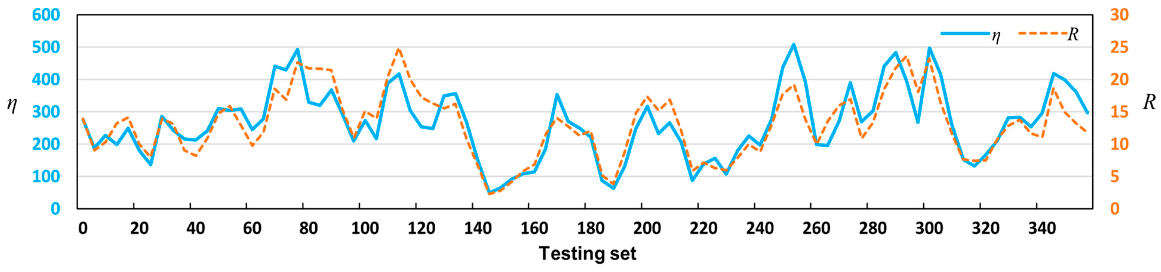
where T = t/4, t ∈ [0, 359], and is the power consumption per hour. The purification efficiency is averaged over 4 h because this is the maximum predictable period for the LMPNet. Figure 9 shows the purification efficiency factor η and the synthesized purification factor R over the hours of the testing set.
It can be seen from Figure 9 that the variations of the purification efficiency factor are well suited to the synthesized purification factor; this is because most of the electricity consumption of the WWTP is for the operation of the pumps and fans, which work in a fixed power mode. This situation results in relatively low energy efficiency when the inflow water quality of CODin and NH3-Nin is relatively low; the energy efficiency can be improved by adjusting the real-time power of the pumps and fans according to the R factor.
5. Conclusions
In this study, the operational data of a WWTP was analyzed and modeled with a deep network of LMPNet. The potential correlation of the operational data, such as the COD, pH, and NH3-N, recorded by a WWTP in southern China, was learned by the LMPNet model. In the experiment, the prediction deviation metrics of MSE, MAE, and R2 were used to measure the prediction performance, and it was shown that the predicted values approximated the true values of the testing data well. In order to maintain the prediction performance of the LMPNet model, a lifelong learning strategy was also developed to ensure high accuracy for the changing environment over time. An ablation experiment was also carried out to analyze the strength of the nonlinear correlation within the input water quality characteristics. It can be seen from the experimental results that the proposed LMPNet has the potential to optimize the operable parameters of wastewater treatment systems in advance by predicting changes in the influent characteristics so as to reduce the energy consumption.
Author Contributions
N.W. envisioned this study for the research articles; J.W., L.Z., Q.Z. and H.Z. were engaged in the planning and recording of data of this study; N.W. and Q.Z. supervised the project; the study was reviewed, drafted, and revised by Z.W. and N.W.; Z.W. and N.W. and performed the experiments on this study; H.H. and Z.W. designed the software; L.Z. and H.Z. acquired funding for this project. All authors have read and agreed to the published version of the manuscript.
Funding
This work is partially supported by the 100 Scholar Plan of the Guangxi Zhuang Autonomous Region (2018) and the Special Fund for Bagui Scholars of the Guangxi (2019A08).
Institutional Review Board Statement
Not applicable.
Informed Consent Statement
Not applicable.
Data Availability Statement
Data are available upon request.
Conflicts of Interest
The authors declare no conflict of interest.
References
- Geissen, V.; Mol, H.; Klumpp, E.; Umlauf, G.; Nadal, M.; van der Ploeg, M.; van de Zee, S.E.A.T.M.; Ritsema, C.J. Emerging Pollutants in the Environment: A Challenge for Water Resource Management. Int. Soil Water Conserv. Res. 2015, 3, 57–65. [Google Scholar] [CrossRef]
- Crini, G.; Lichtfouse, E. Advantages and Disadvantages of Techniques Used for Wastewater Treatment. Environ. Chem. Lett. 2019, 17, 145–155. [Google Scholar] [CrossRef]
- Wang, G.; Li, J.; Sun, W.; Xue, B.; Yinglan, A.; Liu, T. Non-Point Source Pollution Risks in a Drinking Water Protection Zone Based on Remote Sensing Data Embedded within a Nutrient Budget Model. Water Res. 2019, 157, 238–246. [Google Scholar] [CrossRef]
- Li, W.; Li, L.; Qiu, G. Energy Consumption and Economic Cost of Typical Wastewater Treatment Systems in Shenzhen, China. J. Clean. Prod. 2017, 163, S374–S378. [Google Scholar] [CrossRef]
- Jin, L.; Zhang, G.; Tian, H. Current State of Sewage Treatment in China. Water Res. 2014, 66, 85–98. [Google Scholar] [CrossRef] [PubMed]
- Garrido-Baserba, M.; Corominas, L.; Cortés, U.; Rosso, D.; Poch, M. The Fourth-Revolution in the Water Sector Encounters the Digital Revolution. Environ. Sci. Technol. 2020, 54, 4698–4705. [Google Scholar] [CrossRef] [PubMed]
- Jain, S.; Shukla, S.; Wadhvani, R. Dynamic Selection of Normalization Techniques Using Data Complexity Measures. Expert Syst. Appl. 2018, 106, 252–262. [Google Scholar] [CrossRef]
- Zhao, X.; Liu, J.; Liu, Q.; Tillotson, M.R.; Guan, D.; Hubacek, K. Physical and Virtual Water Transfers for Regional Water Stress Alleviation in China. Proc. Natl. Acad. Sci. USA 2015, 112, 1031–1035. [Google Scholar] [CrossRef] [Green Version]
- Matheri, A.N.; Ntuli, F.; Ngila, J.C.; Seodigeng, T.; Zvinowanda, C. Performance Prediction of Trace Metals and Cod in Wastewater Treatment Using Artificial Neural Network. Comput. Chem. Eng. 2021, 149, 107308. [Google Scholar] [CrossRef]
- Han, H.; Liu, Z.; Hou, Y.; Qiao, J. Data-Driven Multiobjective Predictive Control for Wastewater Treatment Process. IEEE Trans. Ind. Inf. 2020, 16, 2767–2775. [Google Scholar] [CrossRef]
- Farhi, N.; Kohen, E.; Mamane, H.; Shavitt, Y. Prediction of Wastewater Treatment Quality Using LSTM Neural Network. Environ. Technol. Innov. 2021, 23, 101632. [Google Scholar] [CrossRef]
- Jawad, J.; Hawari, A.H.; Javaid Zaidi, S. Artificial Neural Network Modeling of Wastewater Treatment and Desalination Using Membrane Processes: A Review. Chem. Eng. J. 2021, 419, 129540. [Google Scholar] [CrossRef]
- Jones, R.A.; Lee, G.F. Recent Advances in Assessing Impact of Phosphorus Loads on Eutrophication-Related Water Quality. Water Res. 1982, 16, 503–515. [Google Scholar] [CrossRef]
- Barker, P.S.; Dold, P.L. General Model for Biological Nutrient Removal Activated-Sludge Systems: Model Presentation. Water Environ. Res. 1997, 69, 969–984. [Google Scholar] [CrossRef]
- Bunce, J.T.; Ndam, E.; Ofiteru, I.D.; Moore, A.; Graham, D.W. A Review of Phosphorus Removal Technologies and Their Applicability to Small-Scale Domestic Wastewater Treatment Systems. Front. Environ. Sci. 2018, 6, 8. [Google Scholar] [CrossRef] [Green Version]
- Yaqub, M.; Asif, H.; Kim, S.; Lee, W. Modeling of a Full-Scale Sewage Treatment Plant to Predict the Nutrient Removal Efficiency Using a Long Short-Term Memory (LSTM) Neural Network. J. Water Process Eng. 2020, 37, 101388. [Google Scholar] [CrossRef]
- Nancharaiah, Y.V.; Venkata Mohan, S.; Lens, P.N.L. Recent Advances in Nutrient Removal and Recovery in Biological and Bioelectrochemical Systems. Bioresour. Technol. 2016, 215, 173–185. [Google Scholar] [CrossRef]
- Yan, T.; Ye, Y.; Ma, H.; Zhang, Y.; Guo, W.; Du, B.; Wei, Q.; Wei, D.; Ngo, H.H. A Critical Review on Membrane Hybrid System for Nutrient Recovery from Wastewater. Chem. Eng. J. 2018, 348, 143–156. [Google Scholar] [CrossRef]
- Shen, Y.; Yang, D.; Wu, Y.; Zhang, H.; Zhang, X. Operation Mode of a Step-Feed Anoxic/Oxic Process with Distribution of Carbon Source from Anaerobic Zone on Nutrient Removal and Microbial Properties. Sci. Rep. 2019, 9, 1153. [Google Scholar] [CrossRef] [Green Version]
- Ge, S.; Zhu, Y.; Lu, C.; Wang, S.; Peng, Y. Full-Scale Demonstration of Step Feed Concept for Improving an Anaerobic/Anoxic/Aerobic Nutrient Removal Process. Bioresour. Technol. 2012, 120, 305–313. [Google Scholar] [CrossRef]
- Jeppsson, U.; Pons, M.-N.; Nopens, I.; Alex, J.; Copp, J.B.; Gernaey, K.V.; Rosen, C.; Steyer, J.-P.; Vanrolleghem, P.A. Benchmark Simulation Model No 2: General Protocol and Exploratory Case Studies. Water Sci. Technol. 2007, 56, 67–78. [Google Scholar] [CrossRef]
- Alex, J.; Benedetti, L.; Copp, J.; Gernaey, K.V.; Jeppsson, U.; Nopens, I.; Pons, M.N.; Steyer, J.P.; Vanrolleghem, P. Benchmark Simulation Model No. 1 (BSM1); IWA Publishing: London, UK, 2018; 58p. [Google Scholar]
- Fang, F.; Ni, B.; Li, W.; Sheng, G.; Yu, H. A Simulation-Based Integrated Approach to Optimize the Biological Nutrient Removal Process in a Full-Scale Wastewater Treatment Plant. Chem. Eng. J. 2011, 174, 635–643. [Google Scholar] [CrossRef]
- Cheng, T.; Harrou, F.; Kadri, F.; Sun, Y.; Leiknes, T. Forecasting of Wastewater Treatment Plant Key Features Using Deep Learning-Based Models: A Case Study. IEEE Access 2020, 8, 184475–184485. [Google Scholar] [CrossRef]
- Mohammad, A.T.; Al-Obaidi, M.A.; Hameed, E.M.; Basheer, B.N.; Mujtaba, I.M. Modelling the Chlorophenol Removal from Wastewater via Reverse Osmosis Process Using a Multilayer Artificial Neural Network with Genetic Algorithm. J. Water Process Eng. 2020, 33, 100993. [Google Scholar] [CrossRef]
- Irfan, M.; Waqas, S.; Arshad, U.; Khan, J.A.; Legutko, S.; Kruszelnicka, I.; Ginter-Kramarczyk, D.; Rahman, S.; Skrzypczak, A. Response Surface Methodology and Artificial Neural Network Modelling of Membrane Rotating Biological Contactors for Wastewater Treatment. Materials 2022, 15, 1932. [Google Scholar] [CrossRef] [PubMed]
- Ye, Z.; Yang, J.; Zhong, N.; Tu, X.; Jia, J.; Wang, J. Tackling Environmental Challenges in Pollution Controls Using Artificial Intelligence: A Review. Sci. Total Environ. 2020, 699, 134279. [Google Scholar] [CrossRef]
- Han, H.-G.; Qiao, J.-F.; Chen, Q.-L. Model Predictive Control of Dissolved Oxygen Concentration Based on a Self-Organizing RBF Neural Network. Control. Eng. Pract. 2012, 20, 465–476. [Google Scholar] [CrossRef]
- Suryawan, I.W.K.; Prajati, G.; Afifah, A.S.; Apritama, M.R. NH3-N and COD Reduction in Endek (Balinese Textile) Wastewater by Activated Sludge under Different DO Condition with Ozone Pretreatment. Walailak J. Sci. Technol. 2021, 18, 6. [Google Scholar] [CrossRef]
- Vijayabhanu, R.; Radha, V. Statistical Normalization Techniques for the Prediction of COD Level for an Anaerobic Wastewater Treatment Plant. In Proceedings of the Second International Conference on Computational Science, Engineering and Information Technology—CCSEIT’12, Coimbatore, India, 26–28 October 2012; pp. 232–236. [Google Scholar]
- Mu, Y.; Liu, X.; Wang, L. A Pearson’s Correlation Coefficient Based Decision Tree and Its Parallel Implementation. Inf. Sci. 2018, 435, 40–58. [Google Scholar] [CrossRef]
- Young, S.R.; Rose, D.C.; Karnowski, T.P.; Lim, S.-H.; Patton, R.M. Optimizing Deep Learning Hyper-Parameters through an Evolutionary Algorithm. In Proceedings of the Workshop on Machine Learning in High-Performance Computing Environments, Austin, TX, USA, 15 November 2015; pp. 1–5. [Google Scholar]
- He, K.; Zhang, X.; Ren, S.; Sun, J. Deep Residual Learning for Image Recognition. arXiv 2015, arXiv:1512.03385. [Google Scholar]
- He, T.; Zhang, Z.; Zhang, H.; Zhang, Z.; Xie, J.; Li, M. Bag of Tricks for Image Classification with Convolutional Neural Networks. In Proceedings of the 2019 IEEE/CVF Conference on Computer Vision and Pattern Recognition (CVPR), Long Beach, CA, USA, 15–20 June 2019; pp. 558–567. [Google Scholar]
- Leshno, M.; Lin, V.Y.; Pinkus, A.; Schocken, S. Multilayer Feedforward Networks with a Nonpolynomial Activation Function Can Approximate Any Function. Neural Netw. 1993, 6, 861–867. [Google Scholar] [CrossRef] [Green Version]
- Hochreiter, S.; Schmidhuber, J. Long Short-Term Memory. Neural Comput. 1997, 9, 1735–1780. [Google Scholar] [CrossRef] [PubMed]
- Yan, W.; Xu, R.; Wang, K.; Di, T.; Jiang, Z. Soft Sensor Modeling Method Based on Semisupervised Deep Learning and Its Application to Wastewater Treatment Plant. Ind. Eng. Chem. Res. 2020, 59, 4589–4601. [Google Scholar] [CrossRef]
- Zhang, D. A Coefficient of Determination for Generalized Linear Models. Am. Stat. 2017, 71, 310–316. [Google Scholar] [CrossRef]
- Liu, Y.; Su, Y.; Liu, A.-A.; Schiele, B.; Sun, Q. Mnemonics Training: Multi-Class Incremental Learning Without Forgetting. In Proceedings of the 2020 IEEE/CVF Conference on Computer Vision and Pattern Recognition (CVPR), Seattle, WA, USA, 13–19 June 2020; pp. 12242–12251. [Google Scholar]
- Kingma, D.P.; Ba, J. Adam: A Method for Stochastic Optimization. arXiv 2017, arXiv:1412.6980. [Google Scholar]
Figure 1.
Schematic diagram of the wastewater treatment system based on dual-mode dynamic separation.
Figure 1.
Schematic diagram of the wastewater treatment system based on dual-mode dynamic separation.

Figure 2.
The original values of the 12 water quality parameters measured by sensors from February to June 2022 and used for the preparation of the training and validation sets, including CODin, CODout, pHin, pHout, NH3-Nin, NH3-Nout, F1run, F2run, DO, temperature, Power1h, and outflow.
Figure 2.
The original values of the 12 water quality parameters measured by sensors from February to June 2022 and used for the preparation of the training and validation sets, including CODin, CODout, pHin, pHout, NH3-Nin, NH3-Nout, F1run, F2run, DO, temperature, Power1h, and outflow.

Figure 3.
Pearson’s correlation of the input parameters.

Figure 4.
The structure of the LMPNet model.

Figure 5.
The decrease in the MSE loss value during training at each epoch iteration; the red curve is the training loss, while the blue curve is the validation loss. The minimum validation loss occurs at the 108th epoch with a loss value of 0.183.
Figure 5.
The decrease in the MSE loss value during training at each epoch iteration; the red curve is the training loss, while the blue curve is the validation loss. The minimum validation loss occurs at the 108th epoch with a loss value of 0.183.

Figure 6.
Comparison of the model-predicted and actual values for the untrained testing set with 351 samples at a prediction interval Δt: 9 h.
Figure 6.
Comparison of the model-predicted and actual values for the untrained testing set with 351 samples at a prediction interval Δt: 9 h.

Figure 7.
Comparison of the predicted and actual RE for the untrained testing set with 351 samples at a prediction interval Δt: 9 h.
Figure 7.
Comparison of the predicted and actual RE for the untrained testing set with 351 samples at a prediction interval Δt: 9 h.

Figure 8.
The chart of water quality characteristics in the ablation experiment. The Y-axis is the output features of the LMPNet model, and the X-axis is the input features that were deleted, respectively. The value in the graph is the increase in the output error () after ignoring the corresponding feature, and the larger the value indicates that the input feature is more important to the prediction of the output feature.

Figure 9.
The purification efficiency factor η and the synthesized purification factor R over the hours of the testing set for the WWTP.
Figure 9.
The purification efficiency factor η and the synthesized purification factor R over the hours of the testing set for the WWTP.


Table 1.
Statistics of the original training–validation dataset (n = 3552).
| Water Characteristics and Operating Parameters | ||||
|---|---|---|---|---|
| Variables | Units | Statistics | ||
| Range | Mean | Std | ||
| CODin | mg/L | 53.2–231.6 | 131.6 | 41.5 |
| CODout | mg/L | 14.8–33.16 | 27.0 | 3.5 |
| NH3-Nin | mg/L | 27.5–14.2 | 27.5 | 14.2 |
| NH3-Nout | mg/L | 0.9–10.4 | 7.2 | 2.1 |
| pHin | – | 6.7–7.0 | 6.9 | 0.05 |
| pHout | – | 6.7–7.0 | 6.9 | 0.05 |
| DO | mg/L | 16.3–17.1 | 17 | 0.1 |
| temperature | °C | 25–34.3 | 29.2 | 2.9 |
| Power1h | kW·h | 6.9–15.4 | 10.2 | 1.9 |
| outflow | L/s | 2.5–12.7 | 7.4 | 2.3 |
| F1run | – | 0–1 | 0.52 | 0.48 |
| F2run | – | 0–1 | 0.52 | 0.48 |
Table 2.
The hyperparameters used for the LMPNet model training.
| Hyperparameters | Optimum Values |
|---|---|
| Batch size | 512 |
| Dropout rate | 0.5 |
| Epoch | 120 |
| Optimizer | Adam |
| Learning rate | 0.0003 |
| Weight decay | 0.0001 |
| Train and validation set split ratio | 0.8 |
| Loss function | MSELoss |
Table 3.
The prediction errors of the LMPNet on the output water quality characteristics for different time delays.
Table 3.
The prediction errors of the LMPNet on the output water quality characteristics for different time delays.
| Predicted Water Quality Parameters | ||||||
|---|---|---|---|---|---|---|
| CODout | pHout | NH3-Nout | ||||
| Δt (hour) | MAE | MSE | MAE | MSE | MAE | MSE |
| 6 | 1.299 | 2.440 | 0.053 | 0.005 | 0.761 | 0.958 |
| 8 | 1.143 | 1.936 | 0.055 | 0.006 | 0.645 | 0.671 |
| 10 | 1.306 | 2.584 | 0.054 | 0.005 | 0.698 | 0.800 |
| 12 | 1.67 | 4.346 | 0.051 | 0.005 | 0.905 | 1.388 |
| 14 | 1.992 | 6.146 | 0.046 | 0.004 | 1.116 | 2.086 |
| 16 | 2.342 | 8.287 | 0.038 | 0.003 | 1.415 | 3.075 |
Disclaimer/Publisher’s Note: The statements, opinions and data contained in all publications are solely those of the individual author(s) and contributor(s) and not of MDPI and/or the editor(s). MDPI and/or the editor(s) disclaim responsibility for any injury to people or property resulting from any ideas, methods, instructions or products referred to in the content. |
© 2023 by the authors. Licensee MDPI, Basel, Switzerland. This article is an open access article distributed under the terms and conditions of the Creative Commons Attribution (CC BY) license (https://creativecommons.org/licenses/by/4.0/).
Share and Cite
MDPI and ACS Style
Wei, Z.; Wu, N.; Zou, Q.; Zou, H.; Zhu, L.; Wei, J.; Huang, H. Data Modeling of Sewage Treatment Plant Based on Long Short-Term Memory with Multilayer Perceptron Network. Water 2023, 15, 1472. https://doi.org/10.3390/w15081472
AMA Style
Wei Z, Wu N, Zou Q, Zou H, Zhu L, Wei J, Huang H. Data Modeling of Sewage Treatment Plant Based on Long Short-Term Memory with Multilayer Perceptron Network. Water. 2023; 15(8):1472. https://doi.org/10.3390/w15081472
Chicago/Turabian StyleWei, Zhengxi, Ning Wu, Qingchuan Zou, Huanxin Zou, Liucun Zhu, Jinzhan Wei, and Hong Huang. 2023. "Data Modeling of Sewage Treatment Plant Based on Long Short-Term Memory with Multilayer Perceptron Network" Water 15, no. 8: 1472. https://doi.org/10.3390/w15081472
Note that from the first issue of 2016, this journal uses article numbers instead of page numbers. See further details here.