Combined Forecasting Model of Precipitation Based on the CEEMD-ELM-FFOA Coupling Model

Abstract

Precipitation prediction is an important technical mean for flood and drought disaster early warning, rational utilization, and the development of water resources. Complementary ensemble empirical mode decomposition (CEEMD) can effectively reduce mode aliasing and white noise interference; extreme learning machines (ELM) can predict non-stationary data quickly and easily; and the fruit fly optimization algorithm (FFOA) has better local optimization ability. According to the multi-scale and non-stationary characteristics of precipitation time series, a new prediction approach based on the combination of complementary ensemble empirical mode decomposition (CEEMD), extreme learning machine (ELM), and the fruit fly optimization algorithm (FFOA) is proposed. The monthly precipitation data measured in Zhengzhou City from 1951 to 2020 was taken as an example to conduct a prediction experiment and compared with three prediction models: ELM, EMD-HHT, and CEEMD-ELM. The research results show that the sum of annual precipitation predicted by the CEEMD-ELM-FFOA model is 577.33 mm, which is higher than the measured value of 572.53 mm with an error of 4.80 mm. The average absolute error is 0.81 and the average relative error is 1.39%. The prediction value of the CEEMD-ELM-FFOA model can closely follow the changing trend of precipitation, which shows a better prediction effect than the other three models and can be used for regional precipitation prediction.

1. Introduction

Precipitation is an important way to supply water resources to a basin or region. The accurate precipitation forecasts are valuable and rather important for the integration of natural hazards forecasting [1,2]. Precipitation is affected by many factors [3,4], such as topography, atmospheric circulation, the underlying surface, and human activities. Precipitation time series often have the characteristics of being multi-scale, nonlinear, and unstable.

With the development of machine learning [5,6], scholars at home and abroad have done a lot of related research on the accurate prediction of precipitation by using machine learning algorithms and achieved fruitful results. Partal et al. used a wavelet fuzzy neural network to predict the daily precipitation of three stations in Turkey [7], and the results show that the prediction accuracy of the neural network model is better than that of the classical multiple regression model. Aksoy et al. studied the prediction of monthly precipitation in arid and semi-arid areas through feedforward back propagation (FFBP), radial basis function, and generalized regression artificial neural network (ANN), and the results show that ANN is effective in predicting precipitation in dry months [8]. Alizamir et al. used an extreme learning machine (ELM), a single hidden layer feedforward neural network, an artificial neural network, genetic programming, and quantile mapping to predict large-scale global precipitation; ELM was superior to all other methods in predicting monthly precipitation [9]. The above research is mainly aimed at the traditional neural network, which is not capable of processing non-stationary data and high-frequency abrupt data, and the prediction error is generally between 5 and 20%, which is the bottleneck to further improving the accuracy. Precipitation data are affected by many factors, and most of them show nonlinear and non-stationarity characteristics in the time scale. Therefore, using a coupling model to reduce the non-stationarity of the original series has become a new way to increase the prediction accuracy of precipitation.

At the end of the last century, Huang proposed a new method of processing non-stationary signals, empirical mode decomposition [10], which has been widely used in various fields of signal processing [11,12]. The CEEMD model [13] is an adaptive EMD derived from empirical mode, which can be decomposed into stationary signals with different characteristic scales depending on the characteristics of the signal itself. In the process of signal reconstruction, two Gaussian white noises with the same amplitude and opposite phase are added at the same time, which solves the prediction error of the high-frequency component of the EMD model and also solves the reconstruction error of the EEMD model and restrains the influence of mode aliasing and residual white noise. Wang et al. constructed the CEEMD-SE-HS-KELM prediction model and applied it to the short-term wind power prediction of a wind farm in China [14]. The RMSE and MAE were 2.16 and 0.39, respectively, which were superior to the EMD-SE-HS-KELM, HS-KELM, KELM, and extreme learning machine (ELM) models. Wang et al. constructed a CEEMD-ARIMA prediction model and conducted experiments with precipitation data from 1960 to 2010 in Ningxia Hui Autonomous Region. The results showed that the accuracy of the CEEMD-ARIMA model was higher than that of the ARIMA model at all time scales. All the above studies show that the time series data preprocessed by the CEEMD model can make a certain contribution to improving the prediction accuracy of a traditional neural network model.

At present, there are two deficiencies in the research on the combination of the CEEMD model and neural networks. First, modeling studies on typical non-stationary series of hydrological data such as precipitation are not comprehensive, and the practicability of constructing coupling models between more types of neural network models and CEEMD models needs to be further studied. Secondly, on the basis of existing studies, a new data analysis model is introduced to further enrich the coupling prediction model. Whether it can improve the accuracy of precipitation prediction is worth further exploration. In order to solve the above problems, the swarm optimization algorithm, the fruit fly optimization algorithm (FFOA), is introduced in this paper, which has the characteristics of simple operation and strong local search ability. Combining CEEMD, ELM, and FFOA, a coupling model to further improve the prediction accuracy is sought. In the first mock exam, the CEEMD is used to decompose the precipitation time series into several intrinsic modal components (IMF components). Then, the hidden layer feedforward neural network is constructed for each IMF component, and the extreme learning machine is used for simulation and prediction. Finally, the Drosophila algorithm is used to optimize the accumulation coefficient between IMF components so that the predicted value is as close as possible to the true value, further improving the accuracy of precipitation prediction. In order to verify the validity of the prediction model, the monthly precipitation at Zhengzhou Station is forecasted, and good results are obtained, which provides a new way for precipitation prediction in the future.

2. Research Method

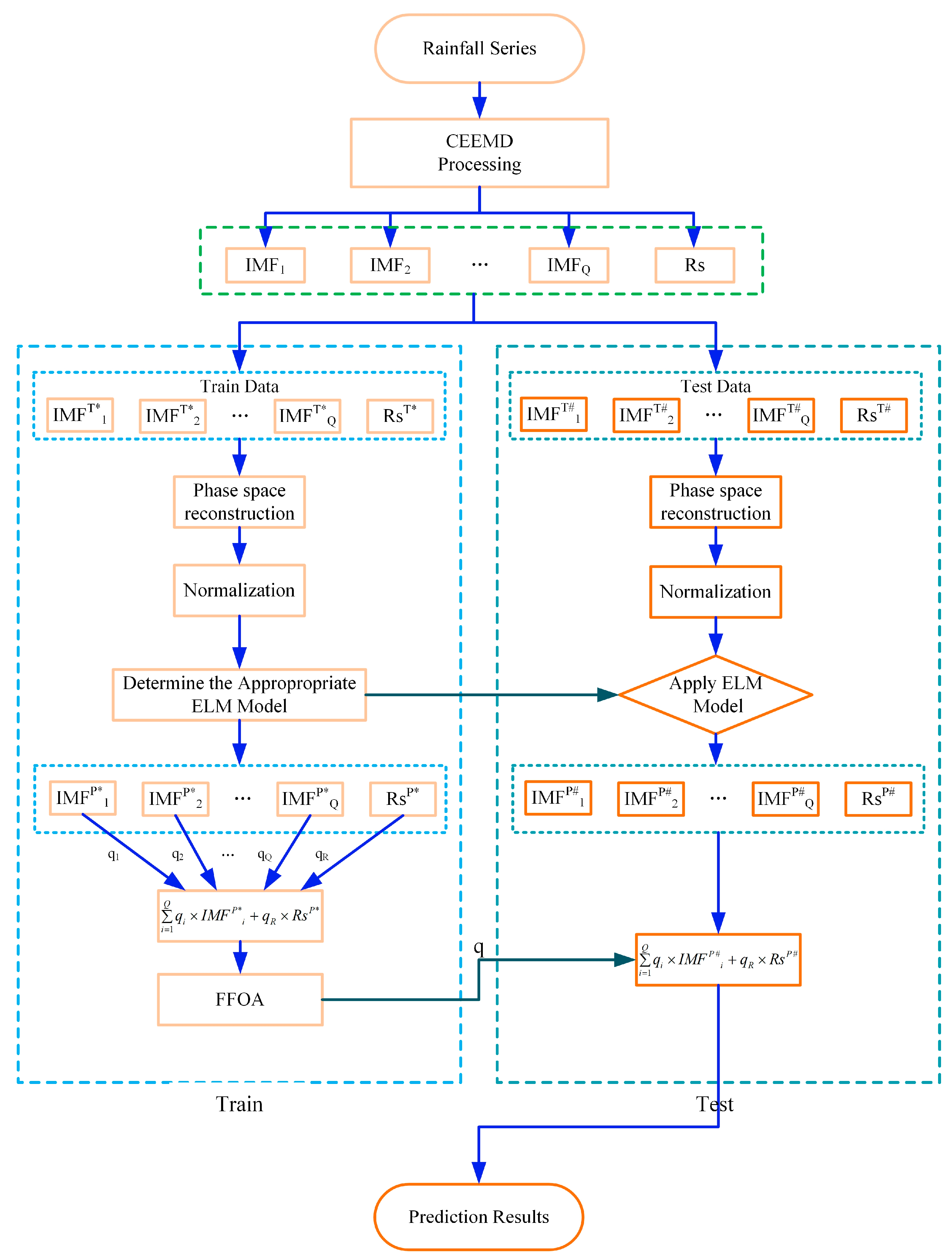
The combined prediction model decomposes complex precipitation prediction problems into relatively simple component prediction problems by CEEMD decomposition, which reduces the difficulty of analysis. At the same time, the model fully considers the contribution of time series information of different scales to the target results and the advantages of ELM in time series prediction, which is conducive to improving precipitation prediction accuracy. In addition, the FFOA method is introduced in the fusion process of the prediction results of each sub-model, and the fusion coefficients of each sub-model are optimized, which further improves the prediction accuracy of the model.

The specific steps of modeling are as follows:

(1) Data preprocessing. Multi-scale decomposition of the original precipitation time series. The CEEMD was used to multi-scale decompose the time series of the seasonal value of the repaired precipitation to obtain Q intrinsic model components $\left(IMF1-IMFQ\right)$ with different frequencies and a residual term $R$;

(2) Intrinsic model components and residual normalization. Phase space reconstruction of each decomposition subsequence. (a) The chaos of each $IMF$ and residual term $R$ are the premise of constructing the prediction model by phase space reconstruction. Therefore, before the reconstruction of phase space, it is necessary to determine whether the Lyapunov exponent of each $IMF$ and residual term $R$ is greater than 0. If it is greater than 0, it means that the time series has chaotic characteristics. This article will use the Wolf method to calculate the maximum Lyapunov exponent of each $IMF$ and residual term $R$. (b) The delay time ${\tau }_{\mathrm{q}}$ of each $IMF$ and residual term $R$ is determined by mutual information method. (c) Determine the embedding dimension $m_q$ of each $IMF$ and residual term $R$ by Cao method. (d) Phase space reconstruction of the one-dimensional time series data set of each $IMF$ and residual term $R$ is performed to obtain the dataset $D_q=\left\{X_i\right.(t),Y_i\left(t\right),t=1,2\cdots ,\left.M\right\}$ in the phase space domain. Normalize the datasets reconstructed in each phase space (Figure 1);

(3) Construction of the ELM prediction model. Establish prediction models for each $IMF$ and residual term $R$. Because the time delay ${\tau }_{\mathrm{q}}$ and the embedded dimension $m_q$ obtained by each decomposition in the phase space reconstruction process are different, it is necessary to establish the prediction model based on the ELM method, respectively, and to reverse normalize the obtained prediction values;

(4) Fusion parameter calculation. The results of each sub-prediction are integrated, and the correlation coefficient of each sub-prediction model is optimized. Using FFOA to optimize the variable coefficients of each sub-prediction model. In optimization, the objective is to minimize the sum of squares of errors, and the variable coefficient optimization problem can be expressed as $\min {{\displaystyle \sum _{t=1}^T\left(y_t-{\displaystyle \sum _{q=1}^{Q+1}{\omega }_q•{\overline{y}}_{qt}}\right)}}^2$.

2.1. Complementary Ensemble Empirical Mode Decomposition

For the analysis and processing of non-stationary signals, Huang et al. proposed the empirical mode decomposition method (EMD) and continuous mean screening method in 1998 [15,16].

CEEMD is a new adaptive decomposition algorithm based on EMD [17] theory and improved on EEMD [18], which was proposed by Yeh et al. [19] in 2010. It can not only effectively overcome the mode aliasing phenomenon in EMD but also eliminate the residual white auxiliary noise added in EEMD to a great extent and improve the computational efficiency of decomposition [20]. The specific steps are as follows:

(1) For a set of raw time series signals $P(t)$, add a pair of Gaussian white noises with the same amplitude and phase ${\omega }^n(t)$, denoting the noise amplitude as ${\beta }_0$, Acquire a new signal $x_i^{+}\left(t\right)$ and $x_i^{-}\left(t\right)$.

$$\left\{\begin{array}{c}{x}_i^{+}\left(t\right)=P\left(t\right)+{\beta }_0{\omega }^n\left(t\right)\\ x_i^{-}\left(t\right)=P\left(t\right)-{\beta }_0{\omega }^n\left(t\right)\end{array}\right.$$

(1)

(2) Using EMD to modal decomposition of new signal group information, A set of intrinsic modal functions ($IMF$) and residual $r_{}(t)$ is obtained. N is the number of intrinsic modal functions.

$$\left\{\begin{array}{c}{x}_i^{+}\left(t\right)={\displaystyle \sum _{j=1}^{N}IM{F}_j^{+i}}+r_i^{+}\left(t\right)\\ x_i^{-}\left(t\right)={\displaystyle \sum _{j=1}^{N}IM{F}_j^{-i}}+r_i^{-}\left(t\right)\end{array}\right.$$

(2)

(3) Varying noise amplitude ${\beta }_0$, Repeat the steps (1) and (2). The mean value of each $IMF$ is calculated according to EMMD. M is the number of positive and negative white noise added.

$$IM{F}_j=\frac{1}{2M}{\displaystyle \sum _{i=1}^M\left(IM{F}_j^{+i}+IM{F}_j^{-i}\right)}$$

(3)

(4) Calculate the residual difference term of CEEMD decomposition. $R(t)$ is the residual component of the original sequence.

$$R\left(t\right)=P\left(t\right)-{\displaystyle \sum _{j=1}^{N}IM{F}_j}$$

(4)

From the above process, the CEEMD decomposition is a process of reconstructing the original signal through multiple Eigen mode extraction. It retains the advantage of EMD in processing non-stationary sequences and makes large noise in the high-frequency components of EMD, thus reducing the reconstruction error caused by the introduction of white noise in EMD. Therefore, it is more suitable for predictive analysis using machine learning.

2.2. Extreme Learning Machine

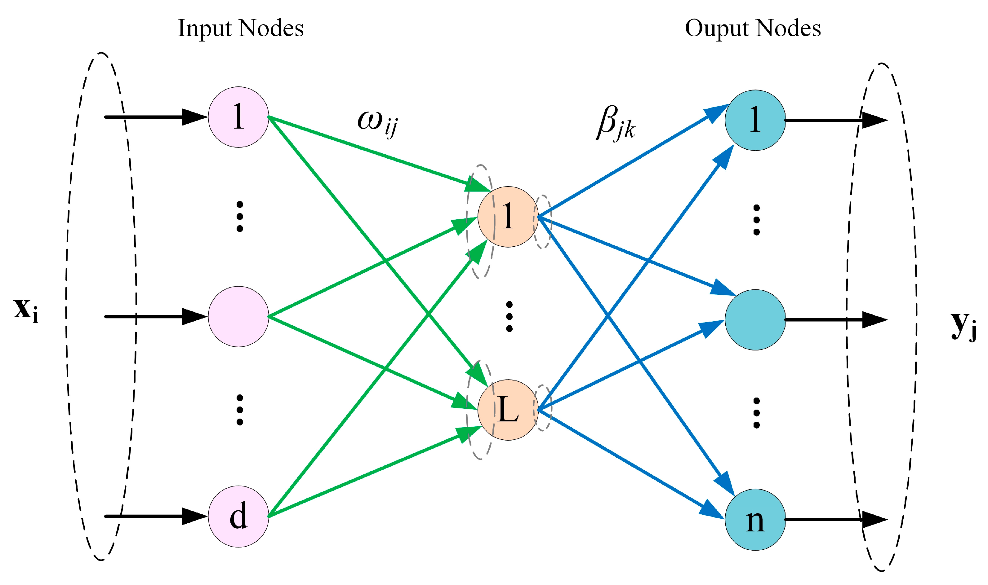
ELM is a machine learning algorithm based on a feedforward neural network [21,22]. ELM can initialize the input weight matrix and bias matrix randomly. Compared with the traditional neural network, ELM can randomly initialize the input weight matrix and bias matrix and has the advantages of strong generalization ability, less manual operation, and fast training speed on the premise of ensuring learning accuracy [23,24,25,26]. The network structure [27] of ELM is shown in Figure 2.

The algorithm has three layers: input layer with $d$ input neurons, hidden layer with $L$ hidden neurons, and output layer with $n$ output neurons.

Give a set of sample data (x, y), where $x_i={\left[x_{i1},\cdots ,x_{in}\right]}^T\in R^n,y_i={\left[t_{i1},\cdots ,t_{im}\right]}^T\in R^m$ has $L$ hidden neurons in the above figure, its network structure can be expressed as [28,29,30]:

$${\displaystyle \sum _{i=1}^L{\beta }_i•g({\omega }_{ij}{x}_j+b_i)=O_j}$$

(5)

where ${\beta }_i=\left[{\beta }_1,{\beta }_2,\cdots ,{\beta }_n\right]$ is the output weight matrix, $g\left(z\right)$ is the activation function, ${\omega }_{ij}$ is the input weight, $b_i$ is the threshold value of the hidden neuron, and $O_j$ is the output result of the extreme learning machine.

A mathematical fitting regression algorithm is to predict the value by infinitely reducing the error. There are ${\beta }_i$, ${\omega }_{ij}$ and $b_i$, that is:

$${\displaystyle \sum _{i=1}^n‖O_j-y_j‖=0}$$

(6)

$${\displaystyle \sum _{i=1}^L{\beta }_i•g({\omega }_{ij}{x}_j+b_i)=y_j}$$

(7)

Equation (7) can be abbreviated as:

$$H\beta =Y$$

(8)

where

$$H={\left[\begin{array}{ccc}g\left(x_1;{\omega }_1;b_1\right)& \cdots & g\left(x_1;{\omega }_L;b_L\right)\\ ⋮& \cdots & ⋮\\ g\left(x_n;{\omega }_1;b_1\right)& \cdots & g\left(x_n;{\omega }_L;b_L\right)\end{array}\right]}_{n\times L},\beta ={\left[\begin{array}{c}{\beta }_1^T\\ ⋮\\ {\beta }_L^T\end{array}\right]}_{L\times \mathrm{m}},T={\left[\begin{array}{c}{y}_1^T\\ ⋮\\ y_n^T\end{array}\right]}_{n\times \mathrm{m}}$$

It can be proved that when the excitation function $g\left(z\right)$ is infinitely differentiable, it is not necessary to adjust all the network parameters.

${\omega }_{ij}$ and $b_i$ are randomly selected at the beginning of training, and it is fixed during training. The output weight matrix ${\beta }_i$ can be obtained by solving the least squares solution of the following equations of linear equations:

$$\beta =H^{+}Y$$

(9)

where $H^{+}$ is the Moore–Penrose generalized inverse of the hidden layer matrix $H^{}$.

2.3. Fruit Fly Optimization Algorithm

Inspired by the foraging behavior of fruit flies, Pan et al. proposed the fruit fly optimization algorithm (FFOA) [31,32]. The basic idea is to use flies superior visual and olfactory senses to locate food; the optimal solution to the problem is searched by iteration. The basic optimization process can be divided into the following steps [33,34,35].

Step (1): Initialize the parameters, set the population size $N$, the maximum number of iterations max, and the position of the fruit fly population $X\_axis$, $Y\_axis$, and give the random direction and distance of each fruit fly individual; then the fruit fly individual begins to search for food using the sense of smell [36,37,38]:

$$\begin{array}{l}{X}_i=X\_axis+Rand\left(\right)\\ Y_i=Y\_axis+Rand\left(\right)\end{array}$$

(10)

where Rand () is the Drosophila flight range, that is, the iterative step size.

Step (2): Preliminary calculation; calculate the distance between each individual fruit fly and the origin of the coordinates $Dis{t}_i$; then calculate the judgment value of the taste concentration of each fruit fly individual $S_i$:

$$\begin{array}{l}Dis{t}_i=\sqrt{X_i^2+Y_i^2}\\ S_i=1/Dis{t}_i\end{array}$$

(11)

Step (3): Localization of olfaction; substituting the taste concentration judgment value $S_i$ in step (2) into fitness function to find the taste concentration of each individual position of the fruit fly $Smel{l}_i$, and find out the fruit fly with the best taste concentration in the fruit fly population (find the maximum value) [39,40,41]:

$$\begin{array}{c}Smel{l}_i=Function\left(S_i\right)\\ \left[\begin{array}{cc}bestSmell& bestIndex\end{array}\right]=\max \left(Smel{l}_i\right)\end{array}$$

(12)

Step (4): Visual orientation; record the taste concentration value and position coordinates of the fruit fly with the best taste concentration. At the same time, the fruit fly population will fly to this position by exerting their visual advantage:

$$\begin{array}{c}bestSmell=bestIndex\\ X\_axis=X\left(bestIndex\right)\\ Y\_axis=Y\left(bestIndex\right)\end{array}$$

(13)

Step (5): Iterative optimization; repeat steps (2) to (3), and determine whether the taste concentration value is bigger than the taste concentration of the previous iteration. If not, repeat the above steps (2) to (3) within the maximum number of iterations; if so, go to step (4).

2.4. Evaluation Method

RE represents the relative percentage error, MAE represents the mean absolute error, RMSE represents the root mean square error, and MAPE represents the mean relative percentage error [42].

$$\mathrm{RE}=\frac{\left|{\mathrm{y}}_{\mathrm{t}}-{\overline{\mathrm{y}}}_{\mathrm{t}}\right|}{{\mathrm{y}}_{\mathrm{t}}}\times 100\%$$

(14)

$$\mathrm{MAE}=\frac{1}{\mathrm{N}}{\displaystyle \sum _{\mathrm{t}=1}^{\mathrm{N}}\left|{\mathrm{y}}_{\mathrm{t}}-{\overline{\mathrm{y}}}_{\mathrm{t}}\right|}$$

(15)

$$\mathrm{RMSE}=\sqrt{\frac{1}{\mathrm{N}}{\displaystyle \sum _{\mathrm{t}=1}^{\mathrm{N}}{({\mathrm{y}}_{\mathrm{t}}-{\overline{\mathrm{y}}}_{\mathrm{t}})}^2}}$$

(16)

$$\mathrm{MAPE}=\frac{1}{\mathrm{N}}{\displaystyle \sum _{\mathrm{t}=1}^{\mathrm{N}}\left|\frac{{\mathrm{y}}_{\mathrm{t}}-{\overline{\mathrm{y}}}_t}{{\mathrm{y}}_{\mathrm{t}}}\right|\times 100\%}$$

(17)

where $y_t$ represents the original value, ${\overline{y}}_t$ represents forecasting value.

RE represents the relative error between a single set of simulated data and the real data. Compared with MAE, RMSE, and MAPE, it can reflect the accuracy of a single predicted value. MAE reaction simulates the average absolute error of multiple data points at one time, which is convenient for comparison between multiple simulations and multiple model simulations. RMSE is squared before calculating the error stack, which is conducive to magnifying the error display. It is convenient to show whether there is excessive error in a set of forecast data. MAPE shows the average relative error of a set of data, is an important parameter to compare the accuracy of prediction, and is suitable for a horizontal comparison of the accuracy of different models. It is worth noting that the smaller the value of these calculation parameters, the smaller the prediction accuracy of the model.

3. Case Study

3.1. Research Area Survey

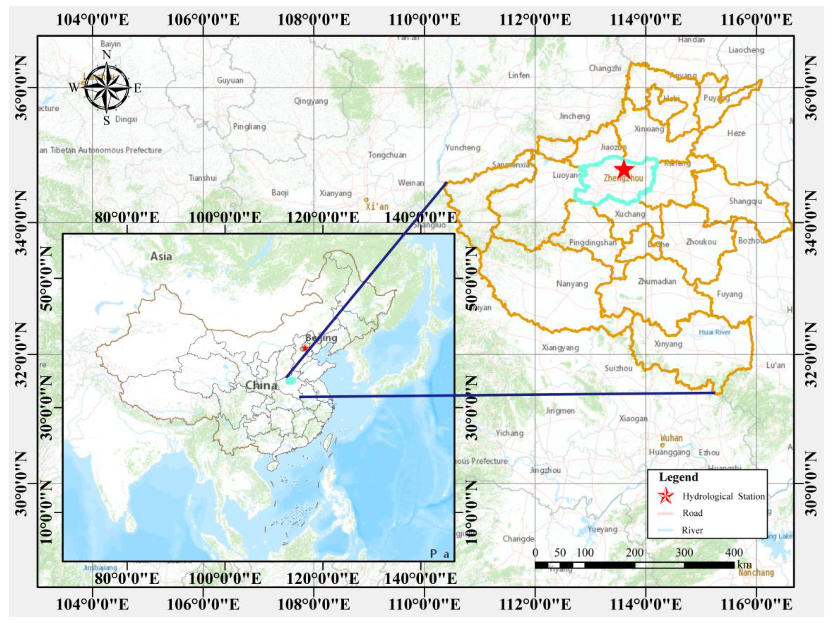
Zhengzhou was chosen as the research area to verify the validity and accuracy of the prediction model. Zhengzhou is the capital city of Henan Province, a megalopolis and the central city of the central plain city, an important central city in central China, and an important comprehensive transportation hub of the country, as approved by the state council. Zhengzhou belongs to the northern temperate continental monsoon climate. The territory of 124 rivers is divided into the Yellow River and Huaihe River systems. The average annual precipitation in Zhengzhou is 636.7 mm; the amount of surface water resources is 494 million cubic meters; and the amount of groundwater resources is 953 million cubic meters. The total amount of water resources is 1.124 billion cubic meters, the amount of water resources per capita is 179 cubic meters, and the amount of water resources per mu is 256 cubic meters. It is an area of severe water shortage. Therefore, the prediction of precipitation in Zhengzhou is of great significance to the regional economic distribution and the effective development and utilization of water resources.

The monthly precipitation sequence of Zhengzhou city in this study is based on the monthly precipitation data of Zhengzhou station from 1951 to 2020 provided by the National Data Center for Meteorological Sciences and Water Resources Bulletin of Zhengzhou. The sequence length was 840 months, the mean value was 48.03 mm, the standard deviation was 67.92 mm, and the maximum precipitation value was 692.2 mm in August 1963. The inter-annual variation of surface precipitation in the study area is shown in Figure 3, Figure 4 and Figure 5. It can be seen from the figure that precipitation in Zhengzhou is generally stable and fluctuates around the mean value of several years in each year. Although precipitation has a decreasing trend, it is not significant, which can be regarded as a non-stationary time series with a weak trend, and this also reflected the reasonability of the selected CEEMD method.

The operating system used in this experiment is Win10, and the deep learning framework is MATLAB2021 b. In terms of hardware, the CPU is eight-core Intel Xeon E5-2630 v4, the memory is 48 G, the GPU is a Nvidia Tesla P100, and the video memory is 16 G.

3.2. Multi-Scale Decomposition of Precipitation Time Series Data Based on CEEMD

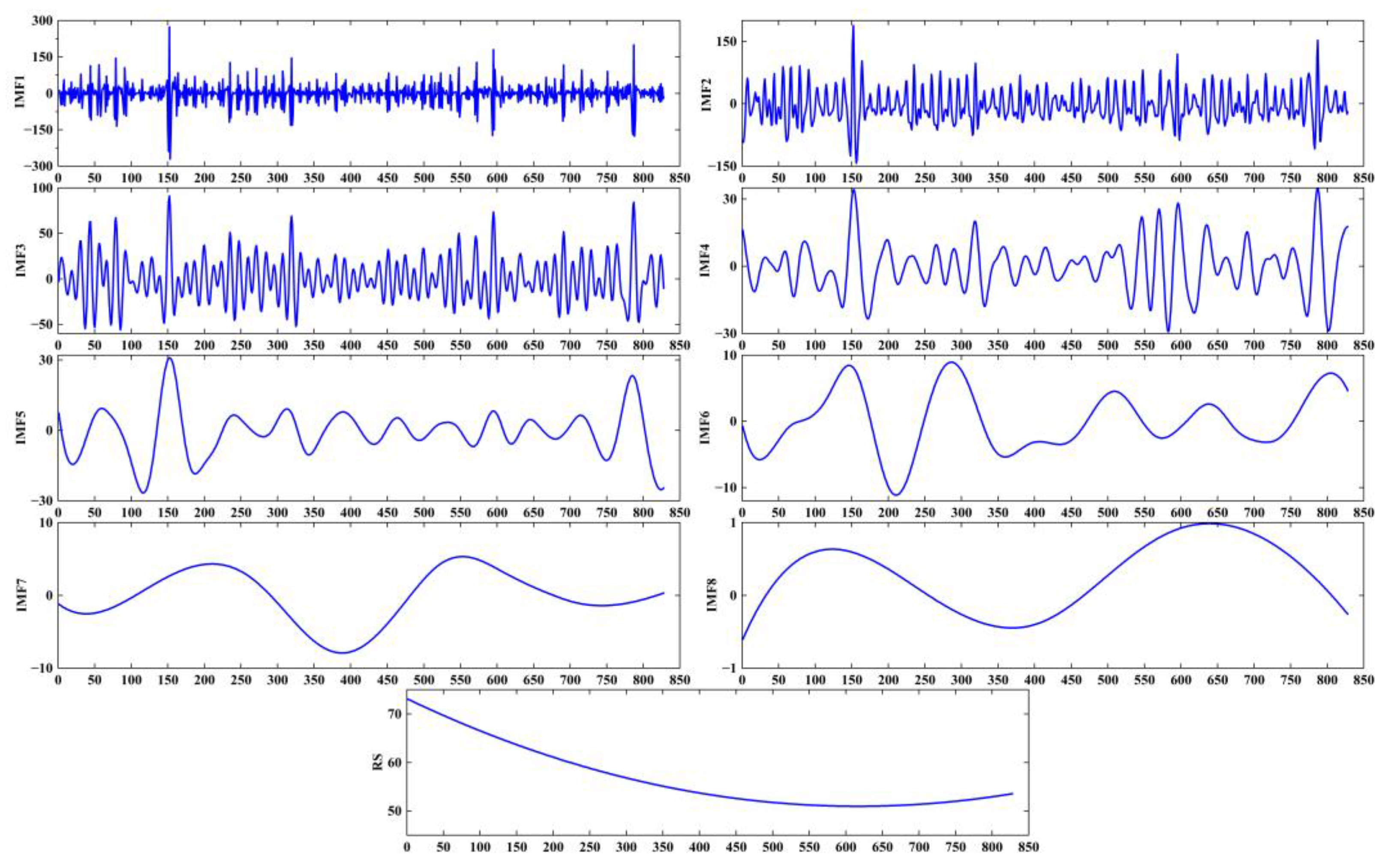
Using the CEEMD algorithm to decompose the original data of the monthly precipitation time series of Zhengzhou from 1951 to 2019, it is found that when the noise amplitude is 0.2 and the noise logarithm is 50, the decomposition effect is ideal. After CEEMD decomposes the time series, eight IMF components and one trend component are obtained, as shown in Figure 5.

As shown in Figure 6, the precipitation time series was divided into eight IMF components and one corresponding trend term, where the IMF1 component underwent the greatest fluctuation with high frequency and the shortest wavelength; the amplitude of IMF2, IMF8, and the trend term were gradually reduced, as were their frequencies, but their wavelengths were gradually increased. After EMD processing, the fluctuation and non-stationarity of the precipitation time series of Zhengzhou were reduced to a great degree, and the original series was decomposed into periodic IMF components in order to relieve the prediction difficulty.

3.3. Model Prediction

Whether the eight IMF components and one trend item obtained by CEEMD decomposition are chaotic time series can be identified by the Lyapunov index method. This paper adopts the mutual information method and the Cao method to obtain the time delay τ_q of each decomposition item and the embedded dimension m_q wolf method to calculate the maximum Lyapunov index of each decomposition amount. The calculation results are shown in

Table 1. Phase space reconstruction information table.

	IMF1	IMF2	IMF3	IMF4	IMF5	IMF6	IMF7	IMF8
τq	2	1	3	6	11	12	15	20
mq	13	12	7	4	2	4	5	2
Lyapunov	0.105	0.0583	0.048	0.0524	0.0936	0.0208	0.0232	0.0335

. The table of the Lyapunov index value greater than 0 illustrates that the decomposition sequence has chaotic characteristics.

Figure 6 shows that after CEEMD decomposition, the volatility and non-stationarity of the time series of annual precipitation in Zhengzhou are greatly reduced, and the training effect of IMF1-IMF8, the real value and predicted value of trend items are getting better and better; the relative error and average relative error of IMF1-IMF8, trend items show a decreasing trend; the training effect of the decomposed high-frequency component IMF1 is slightly poor, while the training effect of the low-frequency component IMF8 and trend item is very good. After the time series of annual precipitation in Zhengzhou is decomposed, the non-stationary nature of the time series is reduced so that ELM can better predict its components and trend term (Figure 7).

3.4. Determining the Correlation Coefficient of Combination of Decomposed Sequences

When the prediction results of each decomposition series are fused, the value of the variable coefficient of each sub-prediction model is related to the influence of the prediction output value of each decomposition series on the final prediction results and determines the final prediction accuracy and performance of the combined model. Therefore, this paper uses Matlab2021b to write the simulation program, the precipitation series of different scales after CEEMD decomposition as the training and test sets, and the variable coefficients of each sub-prediction model are then adaptively trained and optimized by the FFOA algorithm. FFOA initialization: Drosophila population size: Pop = 500; maximum iterations: Maxgen = 10,000. After several experiments, FFOA has achieved better optimization performance, obtained the optimal combination variable coefficients of eight different IMF and residual R sub-prediction models, as shown in

Table 2. Optimization coefficient table.

	IMF1	IMF2	IMF3	IMF4	IMF5	IMF6	IMF7	IMF8	R
Optimization coefficient	1.005	0.987	0.971	1.131	1.126	0.897	0.999	1.073	1.001

.

3.5. Model Validation

The predicted results of IMF1~IMF8 and the trend term were reconstructed into the predicted value of monthly precipitation and compared with the original value of monthly precipitation. The calculated prediction error is shown in

Table 3. Relative error indexes table.

Month	Precipitation		Absolute Error /mm	RE /%
	True Value	Forecasting Value
2020.01	44.40	42.45	1.95	4.40
2020.02	34.60	34.27	0.33	0.96
2020.03	8.40	8.42	0.02	0.19
2020.04	17.00	17.32	0.32	1.87
2020.05	37.50	37.38	0.12	0.32
2020.06	116.90	115.99	0.91	0.78
2020.07	83.70	82.12	1.58	1.89
2020.08	146.03	145.83	0.47	0.32
2020.09	15.60	15.47	0.13	0.81
2020.10	33.90	33.73	0.17	0.49
2020.11	33.50	33.95	0.45	1.35
2020.12	5.80	5.60	0.20	3.38
Mean relative error = 1.39%

.

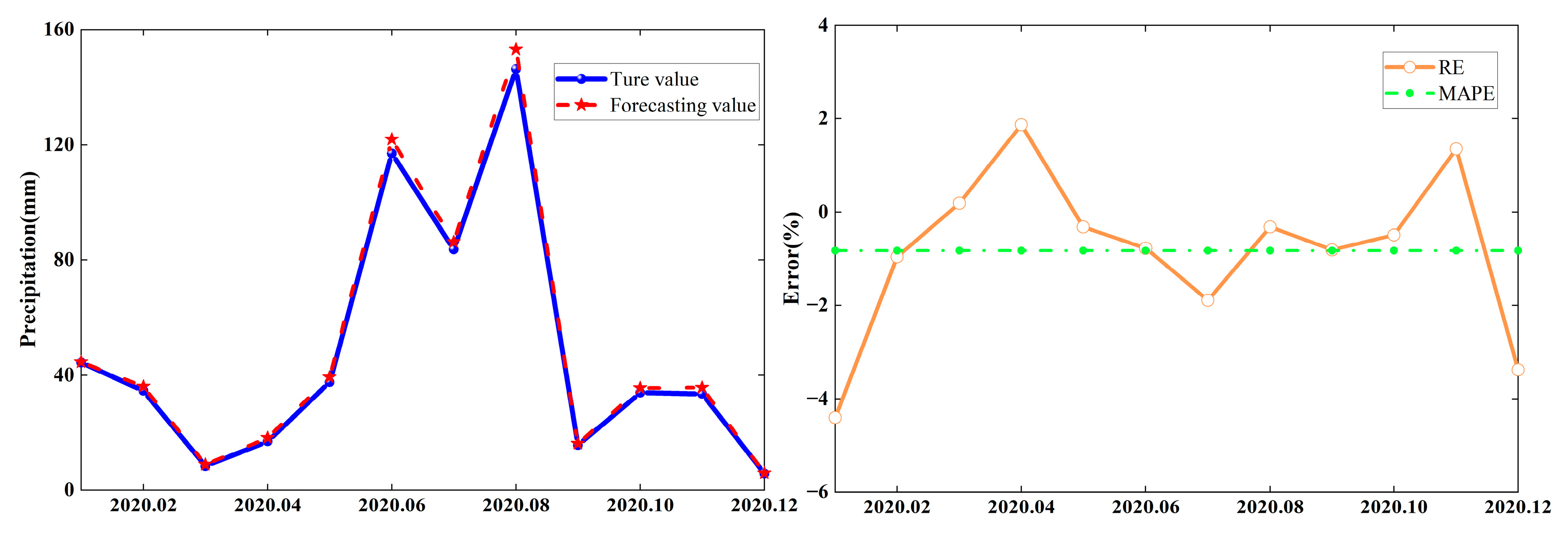
Table 3 illustrates that the maximum value, minimum value, and average value of the relative error of the CEEMD-ELM-FFOA coupling prediction model were 4.40%, 0.19%, and 1.39%, respectively, so the relative prediction error of the model was small with a high eligible rate.

Figure 8 displays the prediction curves of precipitation at Zhengzhou Station during 2020.01–2020.12. It can be seen from Figure 7 that the predicted values are basically consistent with the true values. Therefore, the goodness of fit of the CEEMD-ELM-FFOA coupling model is high and it can be used for regional precipitation prediction.

4. Discussion

In the same period, there has been little research on precipitation using the “decomposition-prediction-reconstruction” coupling method, so reference is made to literature using similar mathematical structure models for comparison. Bo H, et al. proposed a short-term load forecasting method for parks based on complementary integrated empirical mode decomposition (CEEMD), sample entropy, the SBO optimization algorithm, and the least squares support vector regression (LSSVR) model. Taking a park in Liaoning Province as an example, the results show that MAPE is 2.03 and RMSE is 3.14. The calculated errors of MAPE and RMSE in this paper are 1.39% and 0.81, respectively, which are close to each other, confirming the feasibility of establishing such a coupling model.

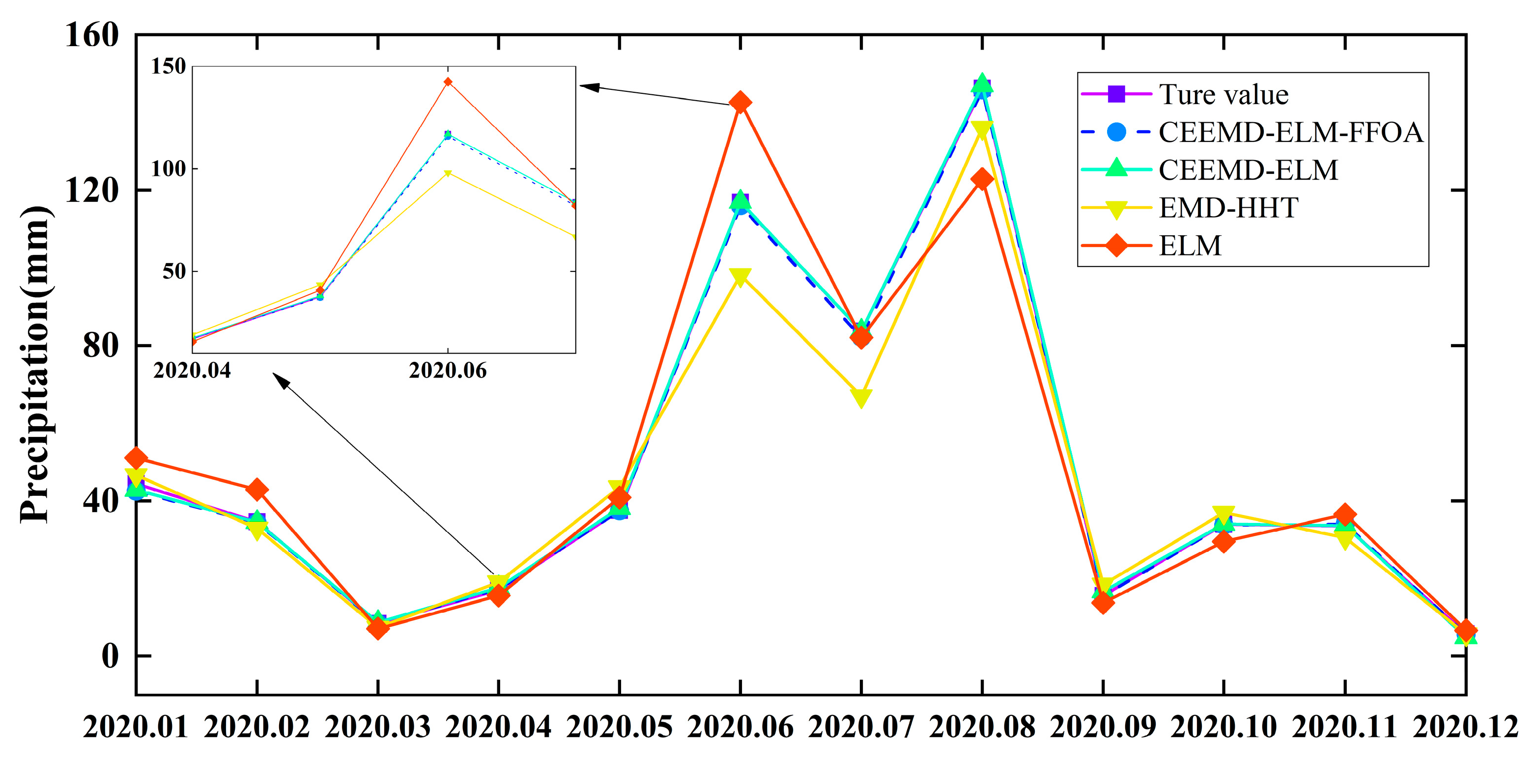
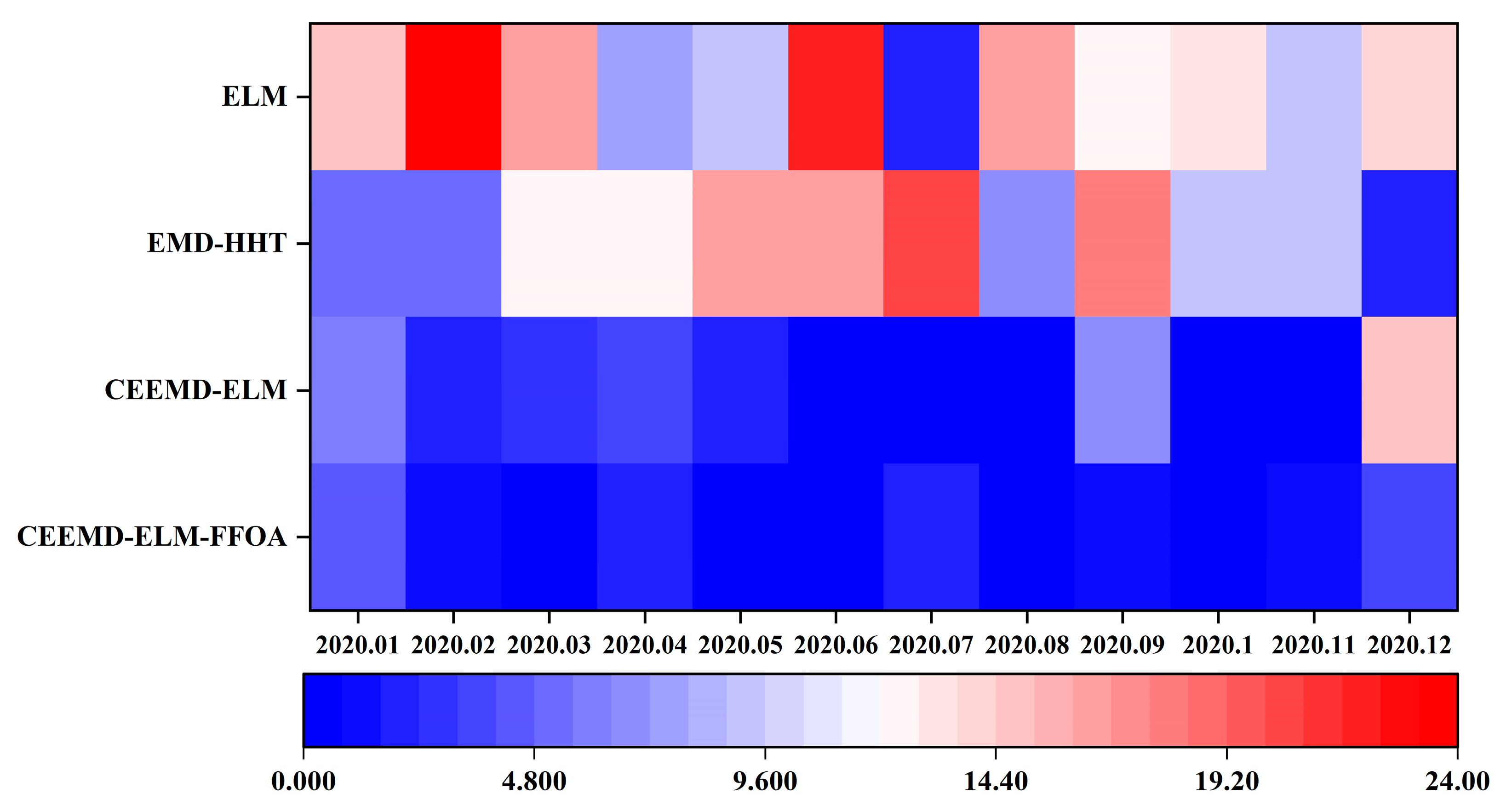
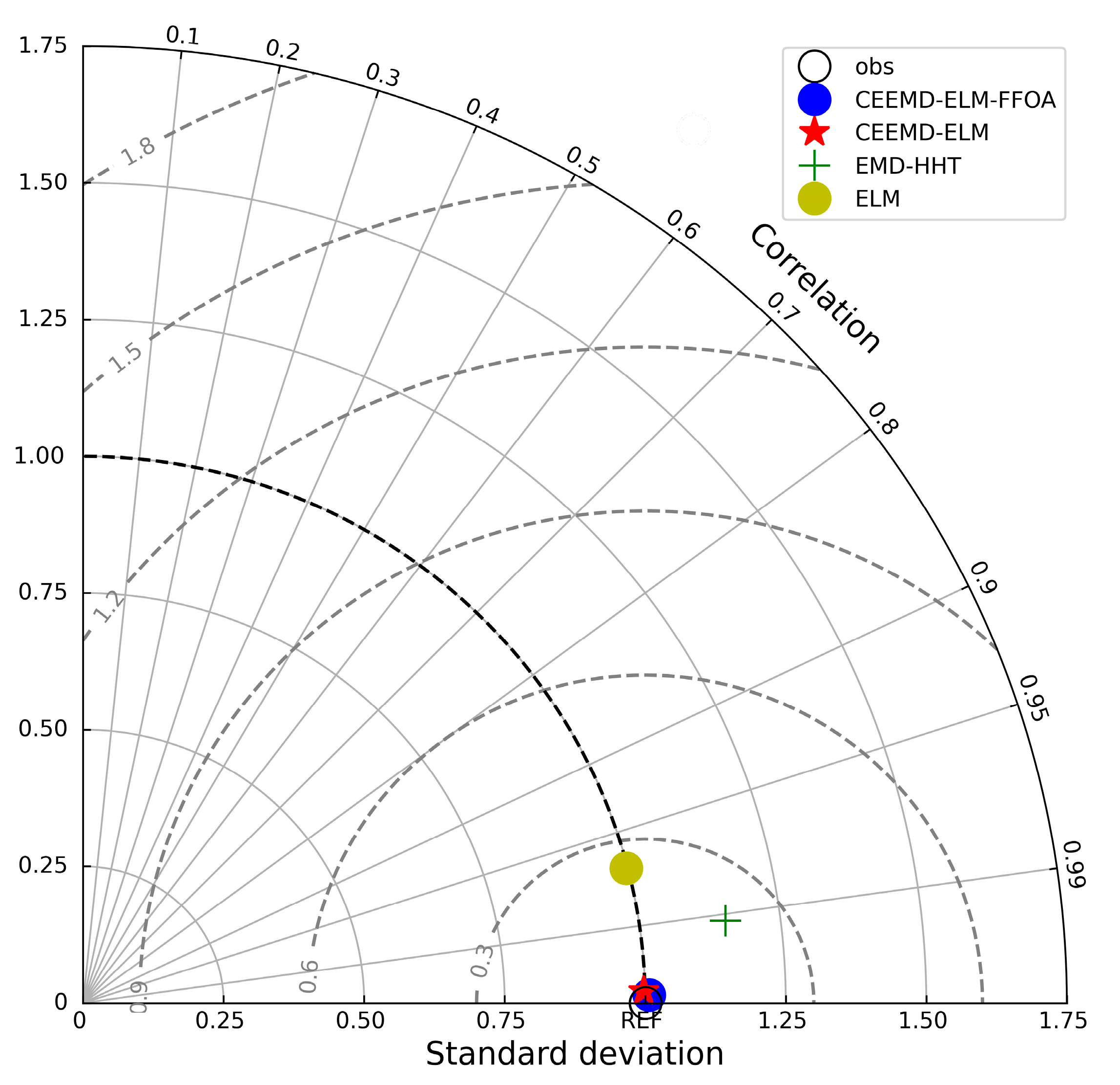
In order to verify the superiority of the CEEMD-ELM-FFOA coupling model in precipitation prediction, the ELM prediction model, the EMD-HHT prediction model, the CEEMD-ELM coupling model, and the CEEMD-ELM-FFOA coupling model were respectively used for prediction, followed by a comparison of their prediction effects. The comparison results of the CEEMD-ELM-FFOA model with other models in prediction error are listed in Figure 9, Figure 10 and Figure 11 and

Table 4. Comparison of evaluation indexes of different models.

Predictive Model	MAE (mm)	RMSE (mm)	MAPE (%)
CEEMD-ELM-FFOA	0.55	0.81	1.39
CEEMD-ELM	0.63	0.92	3.23
EMD-HHT	5.64	8.22	10.92
ELM	6.83	10.70	13.33

.

As shown in Table 4 and Figure 9, Figure 10 and Figure 11, the CEEMD-ELM-FFOA coupling model achieved the highest goodness of fit for predicting precipitation, and its MAE, RMSE, and MAPE were lower than those of the other three prediction models; the goodness of fit of the CEEMD-ELM prediction model was higher than that of the EMD-HHT prediction model. In the meantime, it could be seen that the prediction effect of the “decomposition-prediction-reconstruction” model was remarkably superior to that of a single neural network ELM prediction model. After the decomposition of the original signal, the non-stationarity of the sequence is reduced, the influence of extreme weather conditions on the prediction is weakened, and the prediction accuracy is improved. The prediction accuracy of extreme value is greatly elevated after FFOA optimization and reorganization of data.

The advantages of the CEEMD-ELM-FFOA coupling model mainly focus on its high prediction accuracy, which is consistent with its establishment aim to improve the prediction accuracy on the basis of existing studies. In addition, ELM and FFOA models have the characteristics of simple structure, few parameters, and easy operation, which are also brought into the coupling model. At present, the limitations of this model are mainly reflected in the fact that, compared with the traditional neural network prediction model, although the prediction accuracy is improved, the complexity of the model is increased. For some scenarios that require simple prediction as well as qualitative prediction analysis, the operation is relatively complicated [43]. The applicability of this model in the prediction of other non-stationary hydrological data and the further research focus are to enrich the application range of the model. At the same time, physical parameters affecting precipitation (such as temperature, evaporation, wind speed, etc.) are not considered in this study, and precipitation prediction with these parameters will also become the direction and focus in the future.

5. Conclusions

(1) In order to improve the accuracy of precipitation prediction, this paper uses the empirical model decomposition method, extreme learning machine, and fruit fly optimization algorithm to build a precipitation prediction model based on CEEMD-ELM-FFOA and predicts the monthly precipitation in Zhengzhou. The prediction results show that the model effectively improves the accuracy of precipitation prediction and will predict the change of regional precipitation better;

(2) Multiple sub-time series will be generated after the precipitation time series are decomposed by CEEMD. These sub-time series need to establish their own prediction models to carry out prediction work, and the overall prediction results of the model will be affected by the prediction results of these sub-models. In this paper, FFOA is applied to the fusion of prediction results from sub-models, and the problem of variable coefficient optimization of each sub-model is reasonably solved. The experimental results show that FFOA has a good adaptive optimization ability for variable coefficient optimization and is an effective algorithm for model combination variable coefficient optimization;

(3) The results show that the maximum, minimum, and average relative errors of the CEEMD-ELM-FFOA coupling prediction model are 4.40%, 0.19%, and 1.39%, respectively. The model has a small relative prediction error and a high qualification rate;

(4) Although the overall prediction accuracy of the CEEMD-ELM-FFOA coupling model is high, the phase-space reconstruction method only expands the data dimension from the perspective of statistics. As the input data of the ELM model, it does not consider the physical parameters affecting precipitation (such as temperature, evaporation, wind speed, etc.), which will be the research direction and focus in the next step.

References

- Giannaros, C.; Dafis, S.; Stefanidis, S.; Giannaros, T.M.; Koletsis, I.; Oikonomou, C. Hydrometeorological analysis of a flash flood event in an ungauged Mediterranean watershed under an operational forecasting and monitoring context. Meteorol. Appl. 2022, 29, 2079. [Google Scholar] [CrossRef]
- Kotroni, V.; Cartalis, C.; Michaelides, S.; Stoyanova, J.; Tymvios, F.; Bezes, A.; Christoudias, T.; Dafis, S.; Giannakopoulos, C.; Giannaros, T.; et al. DISARM early warning system for wildfires in the eastern Mediterranean. Sustainability 2022, 12, 6670. [Google Scholar] [CrossRef]
- Trenberth, K.E.; Dai, A.; Rasmuss, R.M.; Parsons, D. The changing character of precipitation. Bull. Am. Meteorol. Soc. 2003, 84, 1205–1218. [Google Scholar] [CrossRef]
- Alexander, L.V.; Zhang, X.B.; Peterson, T.C.; Caesar, J.; Gleason, B.; Tank, A.M.G.K.; Haylock, M.; Collins, D.; Trewin, B.; Rahimzadeh, F.; et al. Global observed changes in daily climate extremes of temperature and precipitation. J. Geophys. Res. Atmos. 2006, 111, 1042–1063. [Google Scholar] [CrossRef] [Green Version]
- Hao, H.; Zhu, H. Application of improved grey waveform prediction method in precipitation prediction. Water Sav. Irrig. 2021, 313, 41–44+50. [Google Scholar]
- Liu, X.; Zhao, N.; Guo, J.Y.; Guo, B. Monthly precipitation prediction of Qinghai Xizang Plateau based on LSTM neural network. J. Earth Inf. Sci. 2020, 22, 1617–1629. [Google Scholar]
- Partal, T.; Kisi, O. Wavelet and neuro-fuzzy conjunction model for precipitation forecasting. J. Hydrol. 2007, 342, 199–212. [Google Scholar] [CrossRef]
- Aksoy, H.; Dahamsheh, A. Markov chain-incorporated and synthetic data-supported conditional artificial neural network models for forecasting monthly precipitation in arid regions. J. Hydrol. 2018, 562, 758–779. [Google Scholar] [CrossRef]
- Alizamir, M.; Moghadam, M.A.; Monfared, A.H.; Shamsipour, A. Statistical downscaling of global climate model outputs to monthly precipitation via extreme learning machine: A case study. Environ. Prog. Sustain. Energy 2018, 37, 1853–1862. [Google Scholar] [CrossRef]
- Huang, N.E.; Shen, Z.; Long, S.R.; Wu, M.C.; Shih, H.H.; Zheng, Q.; Yen, N.-C.; Tung, C.C.; Liu, H.H. The empirical mode decomposition and the Hilbert spectrum for nonlinear and nonstationary time series analysis. Proc. A 1998, 454, 903–995. [Google Scholar]
- Wang, Y.; Dong, R. Low frequency oscillation analysis of multi signal Prony power system with Improved EMD. Control Eng. 2019, 1335–1340. [Google Scholar]
- Xing, W.; Wang, L.P.; Luo, P.P.; Zhao, L.; Weng, Y.; Gao, B. Time frequency matrix DEM noise reduction method based on Wavelet and EMD. J. Xi’an Inst. Aeronaut. 2019, 37, 43–47. [Google Scholar]
- Zhang, J.L.; Liu, Z.Y.; Wang, M.X. Research on natural gas price prediction model based on CEEMD-ELM-ARIMA. Nat. Gas Oil 2021, 39, 129–136. [Google Scholar]
- Wang, K.; Niu, D.; Sun, L.; Zhen, H.; Liu, J.; De, G.; Xu, X. Wind power short-term forecasting hybrid model based on CEEMD-SE Method. Processes 2019, 7, 843. [Google Scholar] [CrossRef] [Green Version]
- Wu, Z.; Huang, N.E.; Long, S.R.; Peng, C.K. On the trend, detrending, and variability of nonlinear and nonstationary time series. Proc. Natl. Acad. Sci. USA 2007, 104, 14889–14894. [Google Scholar] [CrossRef] [PubMed] [Green Version]
- Flandrin, P.; Rilling, G.; Goncalves, P. Empirical mode decomposition as a filter bank. IEEE Signal Process. Lett. 2004, 11, 112–114. [Google Scholar] [CrossRef] [Green Version]
- Damerval, C.; Meignen, S.; Perrier, V. A fast algorithm for bidimensional EMD. IEEE Signal Process. Lett. 2005, 12, 701–704. [Google Scholar] [CrossRef]
- Wu, Z.; Huang, N.E. Ensemble empirical mode decomposition: A noise-assisted data analysis method. Adv. Adapt. Data Anal. 2011, 1, 1–41. [Google Scholar] [CrossRef]
- Yeh, J.R.; Shieh, J.S.; Huang, N.E. Complementary ensemble empirical mode decomposition: A novel noise enhanced data analysis method. Adv. Adapt. Data Anal. 2010, 2, 135–156. [Google Scholar] [CrossRef]
- Wang, D.; Wei, S.; Luo, H.; Yue, C.; Grunder, O. A novel hybrid model for air quality index forecasting based on two-phase decomposition technique and modified extreme learning machine. Sci. Total Environ. 2017, 580, 719–733. [Google Scholar] [CrossRef]
- Huang, G.B.; Zhu, Q.Y.; Siew, C.K. Extreme learning machine: A new learning scheme of feedforward neural networks. In Proceedings of the 2004 IEEE International Joint Conference on Neural Networks (IEEE Cat. No.04CH37541), Budapest, Hungary, 25–29 July 2004; IEEE: Piscataway, NJ, USA, 2005. [Google Scholar]
- Huang, G.B.; Zhu, Q.Y.; Siew, C.K. Extreme learning machine: Theory and applications. Neurocomputing 2006, 70, 489–501. [Google Scholar] [CrossRef]
- Luo, Z.S.; Pan, K.C. Wax deposition rate prediction of waxy crude oil pipelines based on LASSO-ISAPSO-ELM algorithm. Saf. Environ. Eng. 2022, 29, 69–77. [Google Scholar]
- Li, X.; Dong, Z.; Wang, L.; Niu, X.; Yamaguchi, H.; Li, D.; Yu, P. A magnetic field coupling fractional step lattice Boltzmann model for the complex interfacial behavior in magnetic multiphase flows. Appl. Math. Model. 2023, 117, 219–250. [Google Scholar] [CrossRef]
- Gao, C.; Hao, M.; Chen, J.; Gu, C. Simulation and design of joint distribution of rainfall and tide level in Wuchengxiyu Region, China. Urban Clim. 2021, 40, 101005. [Google Scholar] [CrossRef]
- Liu, Y.; Zhang, K.; Li, Z.; Liu, Z.; Wang, J.; Huang, P. A hybrid runoff generation modelling framework based on spatial combination of three runoff generation schemes for semi-humid and semi-arid watersheds. J. Hydrol. 2020, 590, 125440. [Google Scholar] [CrossRef]
- Chen, L.; Wang, S.; Zhang, Y.-H.; Wei, L.; Xu, X.; Huang, T.; Cai, Y.-D. Prediction of nitrated tyrosine residues in protein sequences by extreme learning machine and feature selection methods. Comb. Chem. High Throughput Screen. 2018, 21, 393–402. [Google Scholar] [CrossRef]
- Pan, H.X.; Cheng, G.J.; Cai, L. Comparison of the extreme learning machine with the support vector machine for reservoir permeability prediction. Comput. Eng. Sci. 2010, 32, 131–134. [Google Scholar]
- Mohammed, E.; Hossam, F.; Nadim, O. Improving extreme learning machine by competitive swarm optimization and its application for medical diagnosis problems. Expert Syst. Appl. 2018, 104, 134–152. [Google Scholar]
- Li, L.D.; Cui, D.W. SSA-ELM hydrological time series prediction model based on wavelet packet decomposition and phase space reconstruction. People’s Pearl River, 2022; in process. [Google Scholar]
- Pan, W.T. A new fruit fly optimization algorithm: Taking the financial distress model as an example. Knowl. Based Syst. 2012, 26, 69–74. [Google Scholar] [CrossRef]
- Yue, Z.; Zhou, W.; Li, T. Impact of the Indian Ocean Dipole on Evolution of the Subsequent ENSO: Relative Roles of Dynamic and Thermodynamic Processes. J. Clim. 2021, 34, 3591–3607. [Google Scholar] [CrossRef]
- Huo, H.H. Research on Fruit Fly Optimization Algorithm and Its Applications. Master’s Thesis, Taiyuan University of Technology, Taiyuan, China, 2015. [Google Scholar]
- Hu, R.; Wen, S.; Zeng, Z.; Huang, T. A short-term power load forecasting model based on the generalized regression neural network with decreasing step fruit fly optimization algorithm. Neurocomputing 2017, 221, 24–31. [Google Scholar] [CrossRef]
- Lv, S.X.; Zeng, Y.R.; Wang, L. An effective fruit fly optimization algorithm with hybrid information exchange and its applications. Int. J. Mach. Learn. Cybern. 2018, 9, 1623–1648. [Google Scholar] [CrossRef]
- Xu, D.; Li, J.; Liu, J.; Qu, X.; Ma, H. Advances in continuous flow aerobic granular sludge: A review. Process Saf. Environ. Prot. 2022, 163, 27–35. [Google Scholar] [CrossRef]
- Ge, D.; Yuan, H.; Xiao, J.; Zhu, N. Insight into the enhanced sludge dewaterability by tannic acid conditioning and pH regulation. Sci. Total Environ. 2019, 679, 298–306. [Google Scholar] [CrossRef]
- Yuan, L.; Yang, D.; Wu, X.; He, W.; Kong, Y.; Ramsey, T.S.; Degefu, D.M. Development of multidimensional water poverty in the Yangtze River Economic Belt, China. J. Environ. Manag. 2023, 325, 116608. [Google Scholar] [CrossRef] [PubMed]
- Li, J.; Wang, Z.; Wu, X.; Xu, C.; Guo, S.; Chen, X. Toward Monitoring Short-Term Droughts Using a Novel Daily Scale, Standardized Antecedent Precipitation Evapotranspiration Index. J. Hydrometeorol. 2020, 21, 891–908. [Google Scholar] [CrossRef] [Green Version]
- Wu, X.; Guo, S.; Qian, S.; Wang, Z.; Lai, C.; Li, J.; Liu, P. Long-range precipitation forecast based on multipole and preceding fluctuations of sea surface temperature. Int. J. Climatol. 2022, 42, 8024–8039. [Google Scholar] [CrossRef]
- Yin, L.; Wang, L.; Tian, J.; Yin, Z.; Liu, M.; Zheng, W. Atmospheric Density Inversion Based on Swarm-C Satellite Accelerometer. Appl. Sci. 2023, 13, 3610. [Google Scholar] [CrossRef]
- Stefanos, S.; Stavros, D.; Dimitrios, S. Evaluation of Regional Climate Models (RCMs) Performance in Simulating Seasonal Precipitation over Mountainous Central Pindus (Greece). Water 2020, 12, 2750. [Google Scholar] [CrossRef]
- Xu, K.; Ding, Y.; Liu, H.; Zhang, Q.; Zhang, D. Applicability of a CEEMD-ARIMA Combined Model for Drought Forecasting: A Case Study in the Ningxia Hui Autonomous Region. Atmosphere 2020, 13, 1109. [Google Scholar] [CrossRef]
Figure 1.
The technical route of the CEEMD-ELM-FFOA Coupling Prediction Model (* Marks training data and # marks test data).
Figure 2.
The ELM network structure.
Figure 3.
Location map of the study area.
Figure 4.
Monthly precipitation of Zhengzhou Station during 1951–2020.
Figure 5.
Boxplot of monthly precipitation at Zhengzhou Station during 1951–2020.
Figure 6.
Precipitation CEEMD decomposition in Zhengzhou from 1951 to 2019.
Figure 7.
Prediction results of IMF1-IMF8 and trend term and the errors.
Figure 8.
Precipitation prediction curve of Zhengzhou Station in 2020.
Figure 9.
Prediction results of different models.
Figure 10.
Hot spots of prediction errors of different models.
Figure 11.
Taylor diagrams for statistical comparison of different models.