

Assessment of ERA5-Land Data in Medium-Term Drinking Water Demand Modelling with Deep Learning
by
 , , , and
Pranav Dhawan
*,
Daniele Dalla Torre
,
Ariele Zanfei
,
Andrea Menapace
,
Michele Larcher
 and
and
Maurizio Righetti
Faculty of Engineering, Free University of Bozen-Bolzano, Piazza Università 1, 39100 Bolzano, Italy
*
Author to whom correspondence should be addressed.
Water 2023, 15(8), 1495; https://doi.org/10.3390/w15081495
Submission received: 13 March 2023
/
Revised: 3 April 2023
/
Accepted: 8 April 2023
/
Published: 11 April 2023
(This article belongs to the Special Issue Smart Technologies for Urban Water Systems)
Abstract
:Drinking water demand modelling and forecasting is a crucial task for sustainable management and planning of water supply systems. Despite many short-term investigations, the medium-term problem needs better exploration, particularly the analysis and assessment of meteorological data for forecasting drinking water demand. This work proposes to analyse the suitability of ERA5-Land reanalysis data as weather input in water demand modelling. A multivariate deep learning model based on the long short-term memory architecture is used in this study over a prediction horizon ranging from seven days to two months. The performance of the model, fed by ground station data and ERA5-Land data, is compared and analysed. Close-to-operative forecasting is then presented using observed data for training and ERA5-Land dataset for testing. The results highlight the reliability of the proposed architecture fed by ERA5-Land data for different time horizons. In particular, the ERA5-Land shows promising performance as input of the multivariate machine learning forecasting model, although some meteorological biases are present, which can be improved, especially in close-to-operative application with bias correction techniques. The proposed study leads to practical implications in the use of regional climate model outputs to support drinking water forecasting for sustainable and efficient management of water distribution systems.
1. Introduction
Nowadays, water distribution systems (WDSs) require efficient integrated urban water management solutions for sustainable planning of drinking water use [1,2,3]. Indeed, climate change and rising water demand are forcing the improvement of the water sector to cut resource waste and increase service quality. For this purpose, water demand modelling and forecasting play a crucial role in plenty of different activities, such as optimal pumping scheduling, operational management of tank replenishment and maintenance planning, and achievement of the pressure level required in the water distribution networks [4,5,6]. Furthermore, the increased frequency of drought periods and the decreasing availability of high-quality water have become necessary for medium-term planning to guarantee drinking water equitably, without intermittent services or prohibitive shortages [7,8]. Hence, the need for decision-making processes related to the management of large water basins and the multiple strategic uses of water is forcing the development of medium-term water demand forecasting procedures [9,10,11,12]. Furthermore, to successfully model and forecast medium-term water demand, seasonal climate models which are able to supply weather forecasting are also required, which can be fed into forecasting algorithms. Such datasets are generated by agencies such as Met Office, U.K.; European Centre for Medium-Range Weather Forecasts (ECMWF); National Weather Service, U.S. In addition, also water demand datasets are crucial for many applications, such as burst detection [13,14,15], network model calibration [16,17], state estimation [18,19], and plenty others.
Several methods have been proposed to forecast drinking water demand, which can be broadly categorised into simple statistical and machine learning algorithms. As traditional methods are easy to implement, these methods can be classified into time series and regression models. Some widely implemented time series models are Autoregressive Integrated Moving Average (ARIMA) as adopted by [20] for forecasting daily tank water level for an urban water distribution network in Italy, while [21] evaluated the water budget for three locations in Poland and analysed the trend using such models. Regression models were used by [22] to study the industrial water demand in Beijing, China. However, traditional methods are not able to fully exploit the information of the historical data and their dependence on exogenous variables, such as temperature, wind, and humidity, due to the non-linearity of the problem [23]. Therefore, over the past ten years, the use of machine learning has aided in increasing the performance of water demand modelling and forecasting with accurate and reliable results [24].
Artificial Neural Networks are machine learning tools that cluster, classify, predict, capture, and focus on the functional relationship in historical water demand data [25,26]. Support Vector Regressions (SVR) have also been widely applied for forecasting water demand [27,28]. Several studies have applied these methods to forecast water demand for the short, medium, and long-term. Ref. [29] used four ensemble deep learning models based on four different neural network architectures: Simple Recurrent Neural Network, Long Short-Term Memory (LSTM), Gated Recurrent Unit, and Feed Forward Neural Network, to forecast short-term (hourly and daily) urban drinking water consumption for two case studies in Italy. To tackle the uncertainty related to the variability of the dataset, an ensemble of 10 neural network sub-models of each architecture were generated and stacked, which gave reliable results and outperformed single sub-models. All four architectures were able to produce reliable and robust results. Ref. [30] studied LSTM, SVR, ARIMA, and random forest models to predict water demands for a city in China with temporal resolutions from 15 min to 24 h and concluded that the LSTM model performed better than the other models in predicting water demand for high time resolution. Ref. [31] performed LSTM and Vector Autoregressive Models (VARs) to predict daily water consumption for optimising pump operation. LSTM model was able to differentiate between different days of the week from each other, leading to better performance than VAR due to its characteristic long-term memory. LSTM model was also able to learn from a completely untrained model and required a few days to achieve reasonable results.
Drinking water demand forecasting is affected by several factors, which include population, consumer preferences, habits, household density, water tariff, technological practices, management strategies, etc. [32,33]. In addition to these factors, temperature and precipitation are the most significant weather variables which impact the water demand behaviour [34,35,36,37]. Varying temperatures and precipitation change the water request, with a negative dependence between precipitation and water use [37,38] and a positive relationship between temperature and water use. Refs. [39,40,41] compared the performance of three models to forecast water demand, with and without weather inputs, with one day lead time for different water supply zones in the Netherlands and concluded that using weather variables improved the performance of the models, which can be of relevance when higher accuracy of forecasting is important. Similar findings were also inferred by [42], which used temperature, rainfall, evaporation, solar radiation, vapour pressure, and relative humidity to forecast the water demand for a catchment in Australia, which provides support to the argument that weather variables affect water demand.
Water demand models use different inputs, and a crucial input for feeding these models are meteorological inputs such as historical datasets (local ground measurement stations) or reanalysis data, which are climate numerical models output based on past data to create the best-modelled data on a fixed spatial and temporal resolution [43,44]. Indeed, reanalysis data are a valid alternative to historical metered data in the areas where the ground stations are present but not complete or their spatial/temporal resolution is not feasible for the application. The reanalysis data used in this paper are ERA5-Land, the ECMWF product produced at the global scale using the land component of the 5th generation of European ReAnalysis (referred to ERA5 hereafter). The high spatial resolution of 9 kilometres, the hourly temporal resolution, and the wide selection of variables available lead to the high interest in this dataset. ERA5 has been used in different fields, such as to model wind power [45], to estimate the surface irradiance [46] and for hydrological modelling [47]. However, the use of ERA5-Land is still a novelty in the water demand field. Indeed, there are no published applications using reanalysis as meteorological forcing for water demand analysis. The same numerical models used to produce climate reanalysis are the core of forecasting data production, with fixed initial conditions and without data assimilation. For example, in the case of ERA5, the seasonal forecasting product is SEAS5 [48]. Therefore, from a practical point of view, ERA5 could be used in the prediction of real drinking water demand as follows: as meteorological input for models training and models validation as hindcast, as a proxy for SEAS5 forecasting meteorological data with only the uncertainty of the Regional Climate Model (RCM) and not the weather forecasts, to test the capability of drinking water models.
Tiwari and Adamowski, 2015 [35] describe long-range water demand forecasting, which works at a time step larger than a month, for planning and design of water supply systems. However, water managers also use medium-term forecasting, which is conducted at a weekly to monthly time horizon, to make informed decisions for managing water resources by balancing the water demand amongst various sectors such as water supply, residential or industrial demands, as well as maintenance activities [35,49]. Moreover, forecasting at hourly, daily, or a time step of less than a week, also known as short-term water demand forecasting, is beneficial for the operational management and optimisation of water supply systems [23,35,39]. Several authors have forecasted water demand in the short term [50,51,52], while a more restricted group in the long term [53,54]. However, medium-term forecasting of water demand is still a concept that has not been fully explored. To the best of the author’s knowledge, no seasonal climate models have been used to support water demand forecasting. Thus, in this paper, drinking water demand in the medium term (from seven days to two months) is forecasted by feeding the ERA5 dataset to a multivariate deep learning model. The performance of the model using the observed dataset and ERA5 will be analysed. In addition, close-to-operative forecasting is also presented using observed data for training and ERA5 data for testing the model to prove the feasibility of ERA5 data as weather input for water demand modelling. Therefore, the purpose of this study is to evaluate ERA5 in feeding deep learning algorithms as a viable option for modelling drinking water demand.
The rest of the paper is divided as follows. Section 2 introduces the case studies with the related data and the methodology developed for the medium-term water demand prediction. Section 3 describes the results of the proposed forecasting method fed by observed and ERA5 weather data, while Section 4 presents the discussion about the suitability of ERA5 data for close-to-operative medium-term forecasting. The final remarks are proposed in Section 5.
2. Materials and Methods
The materials and methods of the proposed work are described hereafter, specifically, Section 2.1 and Section 2.2 present the water demand and the meteorological data, while Section 2.3 introduces the forecasting methodology. In addition, two case studies in the mountainous region of Trentino Alto Adige in the northern part of Italy are selected to compare ERA5 data with observed data in water demand forecasting.
2.1. Water Demand
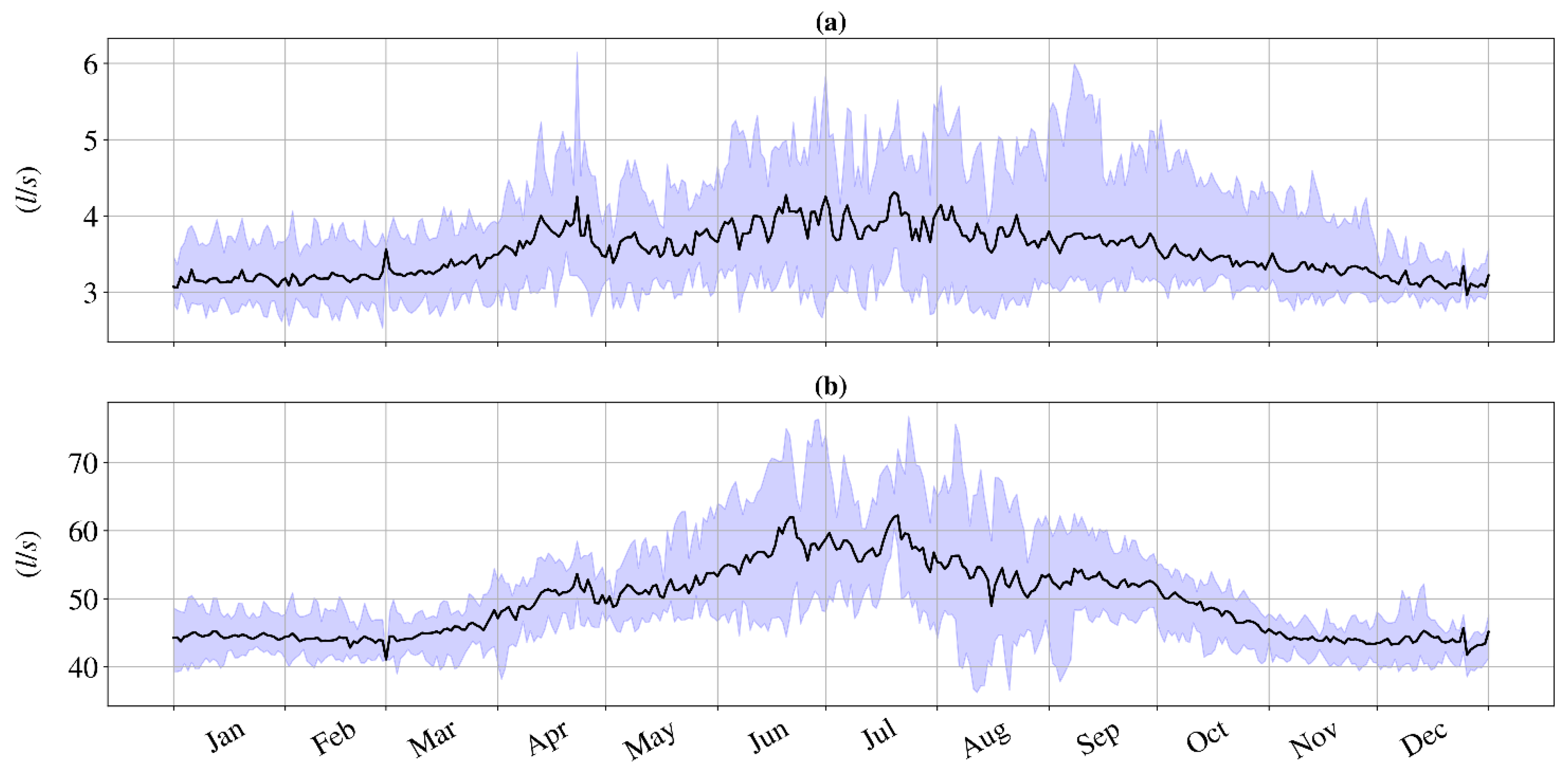
This section introduces the water demand data used in this study. In particular, the demand data belong to two WDSs in the north of Italy. The first case study has almost eight years (from 1 January 2013 to 1 September 2020) of observations, while the second is almost seven years long (from 1 January 2013 to 1 September 2019). Figure 1 shows the daily average value of the demand for both case studies.
In Figure 1a, the black line depicts the daily average value for case study 1 from 2013 to 2020 while Figure 1b depicts case study 2 from 2013 to 2019. The intervals represent the minimum and the maximum water demand registered for each day of the year. The typical seasonal water demand behaviour emerges with a significant yearly periodicity that involves both data level and variability. It is worth mentioning that these case studies are typical of small-medium residential systems. Study area 2 has more water users than study area 1. The variation of the water demand over the year depends on the different water usage from the final users, e.g., more water is consumed during summers due to outdoor water use such as watering of gardens and lawns [55,56], while less is consumed during winters. Table 1 gives the overall summary of the observed data of the two case studies, including the mean, standard deviation, and quantiles.
Concerning the training and testing portion of the dataset, the observations from 1 January 2013 to 1 November 2018 are adopted as training and the remaining almost 2 years as testing for case study 1. Similarly, the data from 1 January 2013 to 1 November 2017 are used as training, while the remaining part is until 1 September 2019 as testing for case study 2.
2.2. Meteorological Data
The weather data used in this work are the measurements of ground stations, and the results of the RCM provided as reanalysis. The measurements of the Autonomous Province of Trento (Italy) of the station of Laste (TN) are the reference dataset for this paper, which was obtained from Meteotrentino. The station of interest represents the area for both the case studies, and the dataset covers the entire period used in this work.
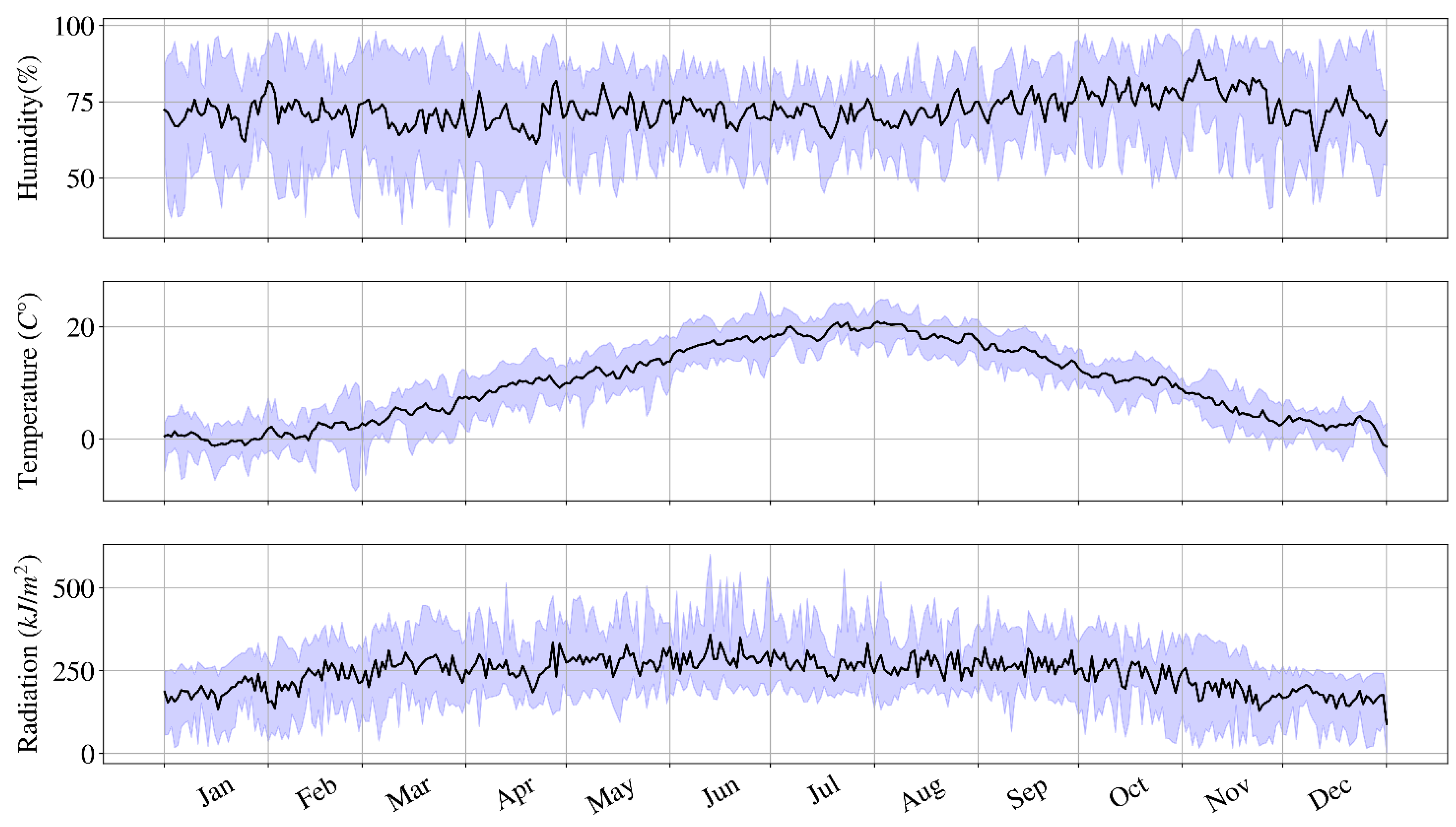
Furthermore, the ERA5 dataset is the main meteorological driver of the forecasting model analysed in this paper. These data are the fifth generation of reanalysis produced by the ECMWF, and the motivation to use them is to evaluate how the model itself is feasible as input of the water demand forecasting models. Indeed, ERA5 and the seasonal forecasting (SEAS5) products of ECMWF are based on the same physical model, but the former provides an enhanced version of the results without the prediction uncertainty. Specifically, the reanalysis dataset includes just the model uncertainties because the data assimilation process and the improved initial condition reduce the other uncertainties (i.e., initial condition and model parameters uncertainties). The ERA5 data are available to download on the Copernicus Climate Change Service Climate Data Store, and the data of interest in this work are the relative humidity (as a combination of 2 m dewpoint temperature and 2 m temperature), solar radiation (surface solar radiation downwards) and temperature (2 m temperature) at hourly temporal resolution and depending on the variable, the data are accumulated or instantaneous values. Figure 2 shows the data at the nearest point of the ERA5 grid to the ground weather station of the two case studies.
The relative humidity does not have a particular pattern, and the mean value is 72% against the 66% of the measurements. The temperature pattern is clear along the year, with ERA5 meanly cooler than ground station values (10 °C vs. 13 °C). The last variable used is the radiation, where a slight pattern along the year is present, with ERA5 that overestimates the real measurements with a mean of 542.88 kJ m−2 against the real value of 520.69 kJ m−2 (shown in Table 2). Although the ERA5 data are a good representation of weather conditions, there are some biases with respect to the measurements, leading to inaccuracy in the inputs of the water demand forecasting algorithm.
2.3. Forecasting Model
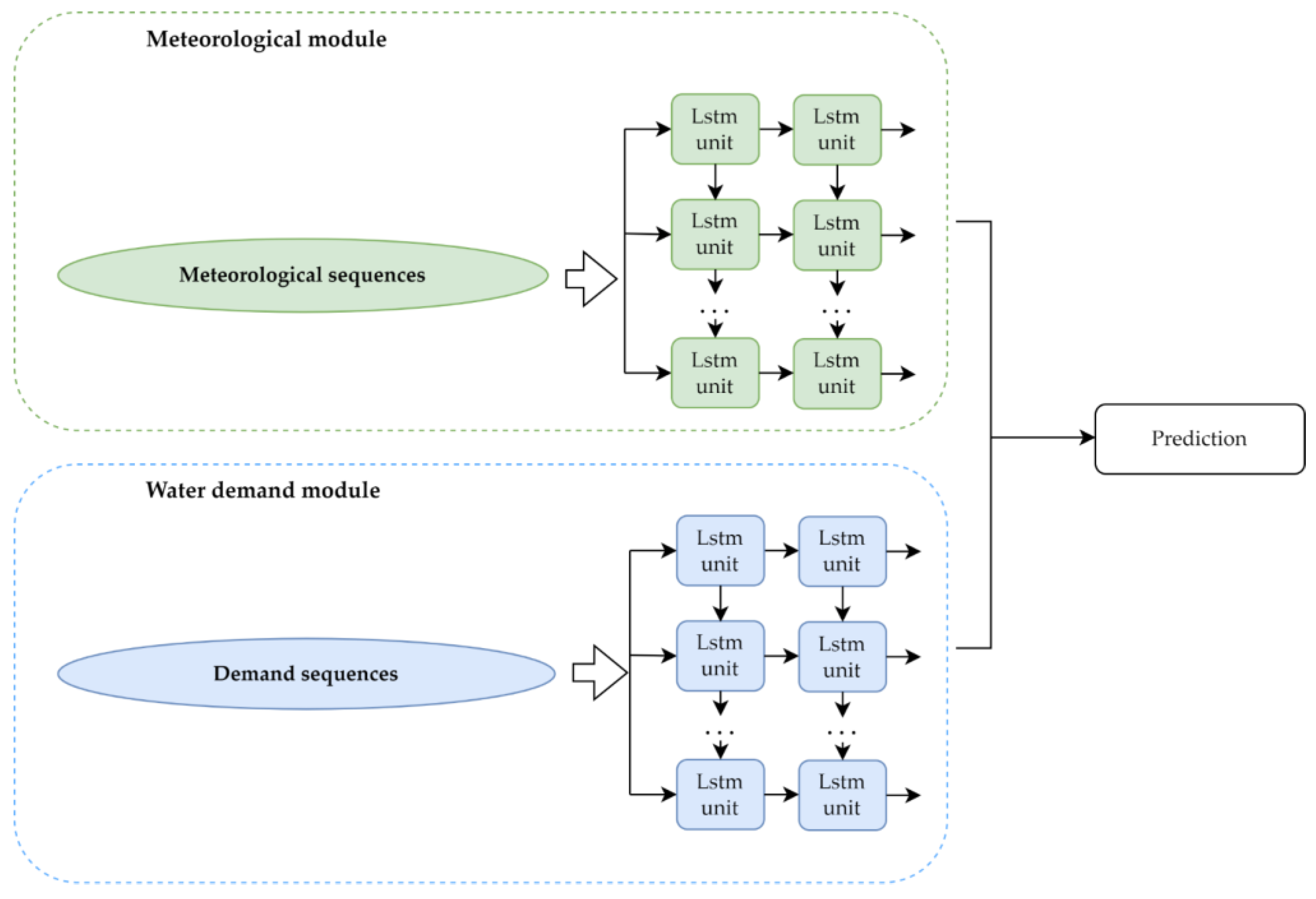
This section presents the model used for this study based on the LSTM units, which have been used with remarkable results for water demand forecasting [57]. Figure 3 presents the architecture of the model, which is the same developed in [57].
The proposed model of Figure 3 has firstly to model the input sequence. This latter is composed of past observations of the water demand and the meteorological variables of relative humidity, temperature, and solar radiation. Therefore, this model is a multivariate LSTM with four different features. Concerning the demand, the sequence is equipped with the past observation of this latter. Differently, the other variables of temperature, humidity, and radiation are forecast data. Generally, this model aims at providing the forecast of daily demand from the time step t until time step t + n, where n is the number of days to be forecasted.
2.4. Evaluation Metrics
The mean absolute error (MAE) and the mean absolute percentage error (MAPE) are adopted to evaluate the prediction ability of the proposed models. These metrics can be defined as follows:
where N is the number of predicted values, yi and are the observed and the forecasted values at the i hourly time step, respectively. It is worth mentioning that the low value of both MAPE and MAE determines a well-performing model.
3. Results
Forecasting of drinking water demand is performed for different time horizons ranging from seven days to two months (i.e., 7, 14, 30, and 60 days). Weather variables (temperature, humidity, and radiation) obtained from ERA5 are used as input to the LSTM deep learning model and are compared with observed data in order to test the feasibility of using ERA5 data as a benchmark for gridded data, which is tested on two case studies.
The model is first trained and tested using observed data to understand the metrics, as discussed in Section 2.1. The results using observed data are shown in Table 4 as “LSTM-OBS”. The shorter time horizon of seven days gives better results than the longer time horizon for both case studies using observed (OBS) data. Next, training and testing of the model are completed on the ERA5 dataset for both case studies (shown in Table 4, “LSTM-ERA5”). The MAE using ERA5 data for seven days is 0.24 L/s and 2.10 L/s for case studies 1 and 2, respectively. Similarly, MAPE for seven days is 6.51% and 3.88% while using ERA5 as input data for both case studies, respectively. However, as the time horizon increases, the efficiency of the model decreases, with MAE increasing from 0.25 L/s to 0.36 L/s from 14 days to 60 days for case study 1 and 2.62 L/s to 4.22 L/s from 14 days to 60 days for case study 2. In order to test the capability of the model, close-to-operative forecasting is performed in which the model is trained using observed data, and testing is carried out using ERA5 data; the results are shown in Table 4 “LSTM-MIX”. The MAE of the close-to-operative model called LSTM-MIX for seven days is 0.31 L/s and 2.49 L/s for case studies 1 and 2, respectively. Similarly, MAPE for seven days for the LSTM-MIX dataset is 8.20% and 4.60% for both case studies, respectively. With an increasing time horizon, MAE increases from 0.25 L/s to 0.36 L/s from 14 days to 60 days for case study 1 and from 3.67 L/s to 3.93 L/s from 14 days to 60 days for case study 2. Similarly, MAPE increases from 9.16% to 9.68% from 14 days to 60 days for case study 1 and from 3.67% to 3.93% from 14 days to 60 days for case study 2.
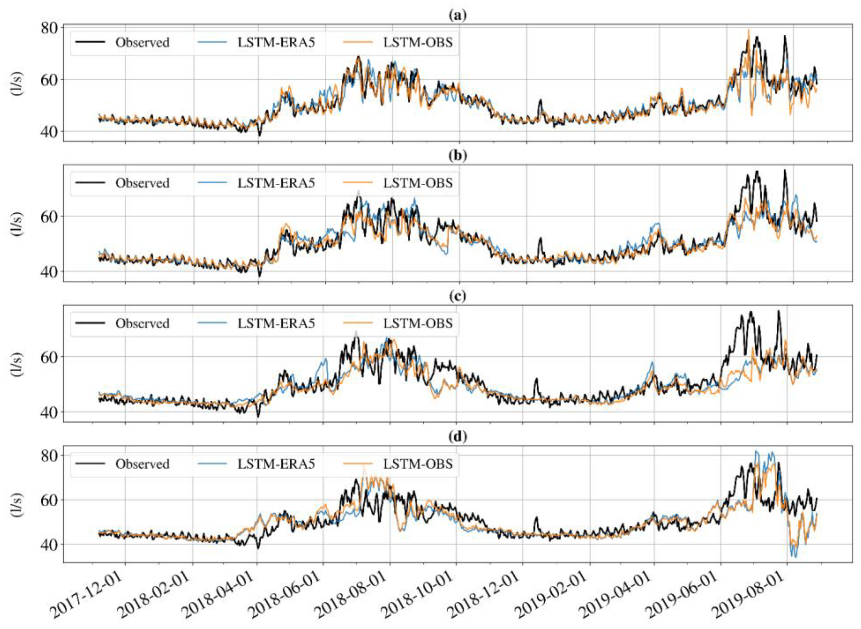
Figure 4 shows the results obtained by the model for case study 2 for different time horizons; in particular, the black line shows the observed drinking water demand, while the orange and blue line shows the modelled drinking water demand for the testing period using observed data and ERA5 data, respectively. Panel a shows the modelled water demand for seven days. Similarly, panels b, c, and d show modelled water demand using different inputs for 14-, 30-, and 60-day horizons for the testing period, respectively. All outputs from the model using different inputs show similar results for the months from October to June. However, for the months from July to September, during high-temperature periods and high variability demand, the model predicts increasing errors with increasing time horizons, with maximum errors for 60 days. The same behaviour of the model can also be seen for study area 1 (see Figure S1 in Supplementary Materials).
4. Discussion
The proposed input of ERA5 to the LSTM model is tested on two study regions, and the results for different combinations, i.e., weather inputs, models, and time horizons, are shown in Table 4. The simulations show better results for case study 2 in all the cases (see Table 4). For example, for the LSTM-OBS to model a seven-day forecast, the MAPE is 6.16% for case study 1 against 3.49% for case study 2. This is due to the higher number of water users in study area 2 than in study area 1, making the demand for case study 2 smoother with less variability and, thus, easier to model and forecast.
Moreover, the behaviour of both case studies is similar, showing a decrease with an increase in the prediction horizon. For this reason, the main discussion in the current section is on case study 2, but it is held to be valid for the other case study. The comparison between observed water demand and modelled water demand using observed and ERA5 data are shown in Figure 4. The LSTM-OBS model leads to a MAPE from 3.49% of the seven days forecasting up to 7.29% at 60 days. It is important to underline that the model with ERA5 input shows similar results with a MAPE from 3.88% (seven days forecasting) up to 7.75% (60 days forecasting). The meteorological bias between the LSTM-OBS and LSTM-ERA5 is reflected in the forecasting outcomes, but this does not invalidate the simulations using ERA5, which seems to be promising.
The LSTM-MIX emphasises the influence of the meteorological input biases, which is even more crucial in a procedure of close-to-operative forecasting where the training data are the observation, while the testing/prediction data are the RCM outputs. The simulations on 7–14 days of forecasting degrade the performance obtained by LSTM-OBS and LSTM-ERA5 models. On the other side, LSTM-MIX on 30- and 60-day time horizon perform in line with LSTM-OBS. It means that the impact of the input data decreases with the increase in the time horizon, and on the contrary, the uncertainty of the LSTM model rises with the growth of the forecasting window. This latter factor does not depend on the input type but only on the forecasting procedure. It can be concluded that the LSTM-ERA5 model can be used as a reference gridded dataset to weather data in the field of drinking water demand forecasting, but the application of a bias correction procedure on the RCM outputs could be helpful to avoid the propagation of the errors in the deep learning algorithm.
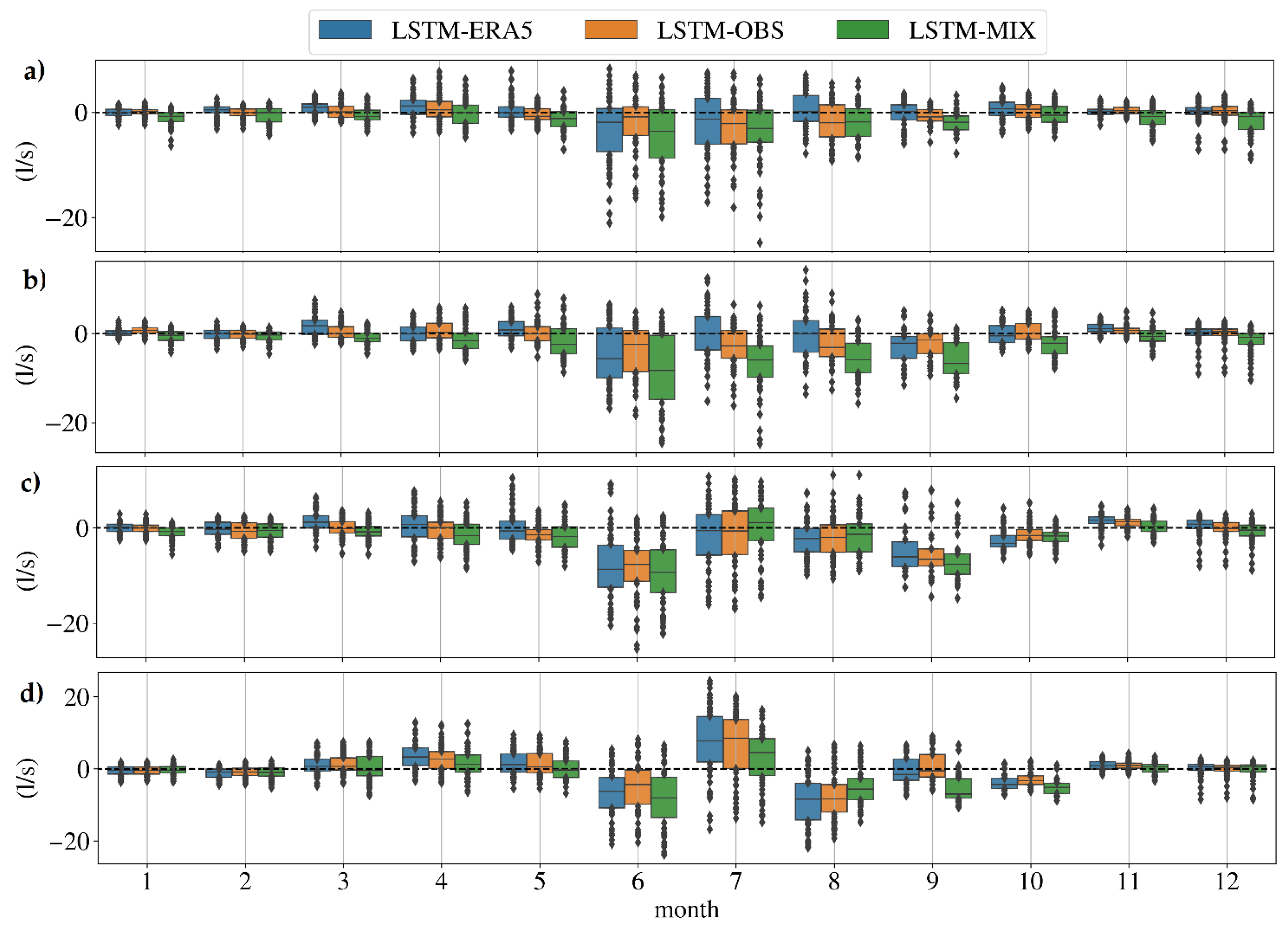
Figure 5 shows the absolute errors for different time horizons for case study 2 using different input datasets. Similar results are obtained for case study 1, which is shown in Supplementary Materials (Figure S2).
In Figure 5, the blue boxes represent the modelled absolute errors using the ERA5 dataset (LSTM-ERA5), observed dataset (orange boxes), and close-to-operative forecasted data (green boxes). The months from October to March show smaller errors. However, higher errors can be seen from June to September due to different seasonality of consumption.
5. Conclusions
Drinking water demand modelling and forecasting are essential for sustainable management and planning of water supply systems. This work aims to evaluate ERA5 in feeding deep learning algorithms as suitable input to model medium-term drinking water demand. A multivariate deep learning model based on the LSTM architecture was adopted to capture the weather data’s time dependencies with water demand. Several simulations were carried out using observed and ERA5 datasets over different time horizons for analyzing the performance of the water demand hindcasting with a particular focus on the suitability of ERA5 reanalysis inputs. In addition, close-to-operative forecasting was also presented, which was trained on the observed data and tested on ERA5 data as a proxy of SEAS5, the seasonal forecasting product of the same RCM provided by ECMWF. The analysis was performed for different time horizons ranging from seven days to two months for two case studies in northern Italy.
With the increase in the time horizon, the uncertainty related to the prediction and its complexity also increased. The LSTM-ERA5 model shows good results when compared to the LSTM-OBS model; however, the meteorological biases of ERA5 lead to slightly worse results. LSTM-MIX emphasises the influence of such biases. For shorter time horizons, the performance of LSTM-MIX is worse than LSTM-OBS and LSTM-ERA5 models. However, for higher time horizons, it is in line with LSTM-OBS, meaning that the impact of the input data decreases with the increase in the time horizon, and the uncertainty of the LSTM model rises with the increase in the forecasting window, which can be attributed to the forecasting procedure and not the input data. Thus, it can be concluded that ERA5 can be used as a reference gridded dataset to weather data to model and forecast drinking water demand. Moreover, it could be significant to use bias correction methods on RCM outputs to avoid propagation errors in the deep learning algorithms, which could be studied in future studies. Due to the use of data from two real-world case studies to model and forecast water demand, it can be concluded that this methodology can be an effective tool for modelling water demand at the medium-term horizon.
Supplementary Materials
The following supporting information can be downloaded at: https://www.mdpi.com/article/10.3390/w15081495/s1. This section reports the results also for case study 1 in terms of forecasting in Figure S1 and in terms of variability of the error in Figure S2.
Author Contributions
Conceptualization, P.D., D.D.T., A.Z., A.M., M.L. and M.R.; data curation, P.D., D.D.T., A.Z. and A.M.; formal analysis, P.D., D.D.T., A.Z. and A.M.; funding acquisition, M.L. and M.R.; investigation, P.D., D.D.T., A.Z. and A.M.; methodology, A.Z. and A.M.; project administration, M.L. and M.R.; resources, M.L. and M.R.; software, D.D.T. and A.Z.; supervision, M.L. and M.R.; validation, P.D., D.D.T., A.Z. and A.M.; visualization, A.Z.; writing—original draft preparation, P.D., D.D.T., A.Z. and A.M.; writing—review and editing, P.D., D.D.T., A.Z., A.M., M.L. and M.R. All authors have read and agreed to the published version of the manuscript.
Funding
This study has been funded by the project DIADEM, Project Number: 5554, “Data driven anomaly detection for sustainable water and energy smart grids management” of the Free University of Bozen-Bolzano, Italy.
Data Availability Statement
The data presented in this study are available on request from the corresponding author.
Conflicts of Interest
The authors declare no conflict of interest.
References
- Sharif, M.N.; Haider, H.; Farahat, A.; Hewage, K.; Sadiq, R. Water–energy nexus for water distribution systems: A literature review. Environ. Rev. 2019, 27, 519–544. [Google Scholar] [CrossRef]
- Fuertes, P.C.; Alzamora, F.M.; Carot, M.H.; Campos, J.A. Building and exploiting a Digital Twin for the management of drinking water distribution networks. Urban Water J. 2020, 17, 704–713. [Google Scholar] [CrossRef]
- Laucelli, D.; Berardi, L.; Giustolisi, O. WDNetXL: Efficient Research Transfer for Management, Planning and Design of Water Distribution Networks. In Proceedings of the 11th International Conference on Hydroinformatics HIC 2014, New York, NY, USA, 17–21 August 2014. [Google Scholar]
- Butler, D.; Memon, F. Water Demand Management; IWA Publishing: London, UK, 2006. [Google Scholar] [CrossRef]
- Alvisi, S.; Franchini, M. Assessment of predictive uncertainty within the framework of water demand forecasting using the Model Conditional Processor (MCP). Urban Water J. 2017, 14, 1–10. [Google Scholar] [CrossRef]
- Meuleman, A.; Cirkel, G.; Zwolsman, G. When climate change is a fact! Adaptive strategies for drinking water production in a changing natural environment. Water Sci. Technol. 2007, 56, 137–144. [Google Scholar] [CrossRef]
- Delpla, I.; Jung, A.-V.; Baures, E.; Clement, M.; Thomas, O. Impacts of climate change on surface water quality in relation to drinking water production. Environ. Int. 2009, 35, 1225–1233. [Google Scholar] [CrossRef]
- Doll, P.; Jiménez-Cisneros, B.; Oki, T.; Arnell, N.; Benito, G.; Cogley, J.; Jiang, T.; Kundzewicz, Z.; Mwakalila, S.; Nishijima, A. Integrating risks of climate change into water management. Hydrol. Sci. J. 2015, 60, 4–13. [Google Scholar] [CrossRef] [Green Version]
- Joshi, N.; Tamaddun, K.; Parajuli, R.; Kalra, A.; Maheshwari, P.; Mastino, L.; Velotta, M. Future Changes in Water Supply and Demand for Las Vegas Valley: A System Dynamic Approach based on CMIP3 and CMIP5 Climate Projections. Hydrology 2020, 7, 16. [Google Scholar] [CrossRef] [Green Version]
- Babel, M.S.; Maporn, N.; Shinde, V.R. Incorporating Future Climatic and Socioeconomic Variables in Water Demand Forecasting: A Case Study in Bangkok. Water Resour. Manag. 2014, 28, 2049–2062. [Google Scholar] [CrossRef]
- Ougougdal, H.A.; Khebiza, M.Y.; Messouli, M.; Lachir, A. Assessment of Future Water Demand and Supply under IPCC Climate Change and Socio-Economic Scenarios, Using a Combination of Models in Ourika Watershed, High Atlas, Morocco. Water 2020, 12, 1751. [Google Scholar] [CrossRef]
- Zubaidi, S.L.; Ortega-Martorell, S.; Al-Bugharbee, H.; Olier, I.; Hashim, K.S.; Gharghan, S.K.; Kot, P.; Al-Khaddar, R. Urban Water Demand Prediction for a City That Suffers from Climate Change and Population Growth: Gauteng Province Case Study. Water 2020, 12, 1885. [Google Scholar] [CrossRef]
- Righetti, M.; Bort, C.M.G.; Bottazzi, M.; Menapace, A.; Zanfei, A. Optimal Selection and Monitoring of Nodes Aimed at Supporting Leakages Identification in WDS. Water 2019, 11, 629. [Google Scholar] [CrossRef] [Green Version]
- Mohammed, E.G.; Zeleke, E.B.; Abebe, S.L. Water leakage detection and localization using hydraulic modeling and classification. J. Hydroinformatics 2021, 23, 782–794. [Google Scholar] [CrossRef]
- Menapace, A.; Zanfei, A.; Felicetti, M.; Avesani, D.; Righetti, M.; Gargano, R. Burst Detection in Water Distribution Systems: The Issue of Dataset Collection. Appl. Sci. 2020, 10, 8219. [Google Scholar] [CrossRef]
- Zanfei, A.; Menapace, A.; Santopietro, S.; Righetti, M. Calibration Procedure for Water Distribution Systems: Comparison among Hydraulic Models. Water 2020, 12, 1421. [Google Scholar] [CrossRef]
- Lima, G.M.; Brentan, B.M.; Manzi, D.; Luvizotto, E. Metamodel for nodal pressure estimation at near real-time in water distribution systems using artificial neural networks. J. Hydroinformatics 2018, 20, 486–496. [Google Scholar] [CrossRef]
- Xing, L.; Sela, L. Graph Neural Networks for State Estimation in Water Distribution Systems: Application of Supervised and Semisupervised Learning. J. Water Resour. Plan. Manag. 2022, 148, 4022018. [Google Scholar] [CrossRef]
- Giustolisi, O.; Savic, D.A. Advances in data-driven analyses and modelling using EPR-MOGA. J. Hydroinformatics 2009, 11, 225–236. [Google Scholar] [CrossRef]
- Guarnaccia, C.; Tepedino, C.; Viccione, G.; Quartieri, J. Short-Term Forecasting of Tank Water Levels Serving Urban Water Distribution Networks with ARIMA Models. In Frontiers in Water-Energy-Nexus—Nature-Based Solutions, Advanced Technologies and Best Practices for Environmental Sustainability; Springer: Berlin/Heidelberg, Germany, 2020; pp. 25–28. [Google Scholar] [CrossRef]
- Birylo, M.; Rzepecka, Z.; Kuczynska-Siehien, J.; Nastula, J. Analysis of water budget prediction accuracy using ARIMA models. Water Supply 2017, 18, 819–830. [Google Scholar] [CrossRef]
- Wei, S.; Lei, A.; Islam, S.N. Modeling and simulation of industrial water demand of Beijing municipality in China. Front. Environ. Sci. Eng. China 2010, 4, 91–101. [Google Scholar] [CrossRef]
- Guo, G.; Liu, S.; Wu, Y.; Li, J.; Zhou, R.; Zhu, X. Short-Term Water Demand Forecast Based on Deep Learning Method. J. Water Resour. Plan. Manag. 2018, 144, 4018076. [Google Scholar] [CrossRef]
- Rezaali, M.; Quilty, J.; Karimi, A. Probabilistic urban water demand forecasting using wavelet-based machine learning models. J. Hydrol. 2021, 600, 126358. [Google Scholar] [CrossRef]
- Du, B.; Zhou, Q.; Guo, J.; Guo, S.; Wang, L. Deep learning with long short-term memory neural networks combining wavelet transform and principal component analysis for daily urban water demand forecasting. Expert Syst. Appl. 2021, 171, 114571. [Google Scholar] [CrossRef]
- Niknam, A.; Zare, H.K.; Hosseininasab, H.; Mostafaeipour, A.; Herrera, M. A Critical Review of Short-Term Water Demand Forecasting Tools—What Method Should I Use? Sustainability 2022, 14, 5412. [Google Scholar] [CrossRef]
- Herrera, M.; Torgo, L.; Izquierdo, J.; Pérez-García, R. Predictive models for forecasting hourly urban water demand. J. Hydrol. 2010, 387, 141–150. [Google Scholar] [CrossRef]
- Brentan, B.M.; Luvizotto, E., Jr.; Herrera, M.; Izquierdo, J.; Pérez-García, R. Hybrid regression model for near real-time urban water demand forecasting. J. Comput. Appl. Math. 2017, 309, 532–541. [Google Scholar] [CrossRef]
- Zanfei, A.; Menapace, A.; Granata, F.; Gargano, R.; Frisinghelli, M.; Righetti, M. An Ensemble Neural Network Model to Forecast Drinking Water Consumption. J. Water Resour. Plan. Manag. 2022, 148, 4022014. [Google Scholar] [CrossRef]
- Mu, L.; Zheng, F.; Tao, R.; Zhang, Q.; Kapelan, Z. Hourly and Daily Urban Water Demand Predictions Using a Long Short-Term Memory Based Model. J. Water Resour. Plan. Manag. 2020, 146, 5020017. [Google Scholar] [CrossRef]
- Kühnert, C.; Gonuguntla, N.; Krieg, H.; Nowak, D.; Thomas, J. Application of LSTM Networks for Water Demand Prediction in Optimal Pump Control. Water 2021, 13, 644. [Google Scholar] [CrossRef]
- Ajbar, A.; Ali, E.M. Prediction of municipal water production in touristic Mecca City in Saudi Arabia using neural networks. J. King Saud Univ. Eng. Sci. 2015, 27, 83–91. [Google Scholar] [CrossRef] [Green Version]
- Bata, M.H.; Carriveau, R.; Ting, D.S.-K. Short-Term Water Demand Forecasting Using Nonlinear Autoregressive Artificial Neural Networks. J. Water Resour. Plan. Manag. 2020, 146, 04020008. [Google Scholar] [CrossRef]
- Tiwari, M.K.; Adamowski, J. Urban water demand forecasting and uncertainty assessment using ensemble wavelet-bootstrap-neural network models. Water Resour. Res. 2013, 49, 6486–6507. [Google Scholar] [CrossRef]
- Tiwari, M.K.; Adamowski, J.F. Medium-Term Urban Water Demand Forecasting with Limited Data Using an Ensemble Wavelet–Bootstrap Machine-Learning Approach. J. Water Resour. Plan. Manag. 2015, 141, 04014053. [Google Scholar] [CrossRef] [Green Version]
- Shah, S.; Hosseini, M.; Ben Miled, Z.; Shafer, R.; Berube, S. A Water Demand Prediction Model for Central Indiana. In Proceedings of the AAAI Conference on Artificial Intelligence, New Orleans, LA, USA, 2–3 February 2018; Volume 32. [Google Scholar] [CrossRef]
- Roushangar, K.; Alizadeh, F. Investigating effect of socio-economic and climatic variables in urban water consumption prediction via Gaussian process regression approach. Water Sci. Technol. Water Supply 2017, 18, 84–93. [Google Scholar] [CrossRef] [Green Version]
- Parandvash, G.H.; Chang, H. Analysis of long-term climate change on per capita water demand in urban versus suburban areas in the Portland metropolitan area, USA. J. Hydrol. 2016, 538, 574–586. [Google Scholar] [CrossRef]
- Stelzl, A.; Pointl, M.; Fuchs-Hanusch, D. Estimating Future Peak Water Demand with a Regression Model Considering Climate Indices. Water 2021, 13, 1912. [Google Scholar] [CrossRef]
- Fiorillo, D.; Kapelan, Z.; Xenochristou, M.; De Paola, F.; Giugni, M. Assessing the Impact of Climate Change on Future Water Demand using Weather Data. Water Resour. Manag. 2021, 35, 1449–1462. [Google Scholar] [CrossRef]
- Bakker, M.; van Duist, H.; van Schagen, K.; Vreeburg, J.; Rietveld, L. Improving the Performance of Water Demand Forecasting Models by Using Weather Input. Procedia Eng. 2014, 70, 93–102. [Google Scholar] [CrossRef] [Green Version]
- Zubaidi, S.L.; Gharghan, S.K.; Dooley, J.; Alkhaddar, R.M.; Abdellatif, M. Short-Term Urban Water Demand Prediction Considering Weather Factors. Water Resour. Manag. 2018, 32, 4527–4542. [Google Scholar] [CrossRef]
- Parker, W.S. Reanalyses and Observations: What’s the Difference? Bull. Am. Meteorol. Soc. 2016, 97, 1565–1572. [Google Scholar] [CrossRef] [Green Version]
- Muñoz-Sabater, J.; Dutra, E.; Agustí-Panareda, A.; Albergel, C.; Arduini, G.; Balsamo, G.; Boussetta, S.; Choulga, M.; Harrigan, S.; Hersbach, H.; et al. ERA5-Land: A state-of-the-art global reanalysis dataset for land applications. Earth Syst. Sci. Data 2021, 13, 4349–4383. [Google Scholar] [CrossRef]
- Olauson, J. ERA5: The new champion of wind power modelling? Renew. Energy 2018, 126, 322–331. [Google Scholar] [CrossRef] [Green Version]
- Urraca, R.; Huld, T.; Gracia-Amillo, A.; Martinez-De-Pison, F.J.; Kaspar, F.; Sanz-Garcia, A. Evaluation of global horizontal irradiance estimates from ERA5 and COSMO-REA6 reanalyses using ground and satellite-based data. Sol. Energy 2018, 164, 339–354. [Google Scholar] [CrossRef]
- Tarek, M.; Brissette, F.P.; Arsenault, R. Evaluation of the ERA5 reanalysis as a potential reference dataset for hydrological modelling over North America. Hydrol. Earth Syst. Sci. 2020, 24, 2527–2544. [Google Scholar] [CrossRef]
- Johnson, S.J.; Stockdale, T.N.; Ferranti, L.; Balmaseda, M.A.; Molteni, F.; Magnusson, L.; Tietsche, S.; Decremer, D.; Weisheimer, A.; Balsamo, G.; et al. SEAS5: The new ECMWF seasonal forecast system. Geosci. Model Dev. 2019, 12, 1087–1117. [Google Scholar] [CrossRef] [Green Version]
- Ghiassi, M.; Zimbra, D.K.; Saidane, H. Urban Water Demand Forecasting with a Dynamic Artificial Neural Network Model. J. Water Resour. Plan. Manag. 2008, 134, 138–146. [Google Scholar] [CrossRef]
- Antunes, A.; Andrade-Campos, A.; Sardinha-Lourenço, A.; Oliveira, M. Short-term water demand forecasting using machine learning techniques. J. Hydroinformatics 2018, 20, 1343–1366. [Google Scholar] [CrossRef] [Green Version]
- Gagliardi, F.; Alvisi, S.; Kapelan, Z.; Franchini, M. A Probabilistic Short-Term Water Demand Forecasting Model Based on the Markov Chain. Water 2017, 9, 507. [Google Scholar] [CrossRef]
- Mouatadid, S.; Adamowski, J. Using extreme learning machines for short-term urban water demand forecasting. Urban Water J. 2016, 14, 630–638. [Google Scholar] [CrossRef]
- Haque, M.; Rahman, A.; Hagare, D.; Chowdhury, R.K. A Comparative Assessment of Variable Selection Methods in Urban Water Demand Forecasting. Water 2018, 10, 419. [Google Scholar] [CrossRef] [Green Version]
- Behboudian, S.; Tabesh, M.; Falahnezhad, M.; Ghavanini, F.A. A long-term prediction of domestic water demand using preprocessing in artificial neural network. J. Water Supply Res. Technol. 2013, 63, 31–42. [Google Scholar] [CrossRef]
- Adamowski, J.; Chan, H.F.; Prasher, S.O.; Ozga-Zielinski, B.; Sliusarieva, A. Comparison of multiple linear and nonlinear regression, autoregressive integrated moving average, artificial neural network, and wavelet artificial neural network methods for urban water demand forecasting in Montreal, Canada. Water Resour. Res. 2012, 48, W01528. [Google Scholar] [CrossRef]
- Polebitski, A.S.; Palmer, R.N. Seasonal Residential Water Demand Forecasting for Census Tracts. J. Water Resour. Plan. Manag. 2010, 136, 27–36. [Google Scholar] [CrossRef]
- Zanfei, A.; Brentan, B.M.; Menapace, A.; Righetti, M. A short-term water demand forecasting model using multivariate long short-term memory with meteorological data. J. Hydroinformatics 2022, 24, 1053–1065. [Google Scholar] [CrossRef]
- Menapace, A.; Zanfei, A.; Righetti, M. Tuning ANN Hyperparameters for Forecasting Drinking Water Demand. Appl. Sci. 2021, 11, 4290. [Google Scholar] [CrossRef]
- Chollet, F.; Watson, M.; Bursztein, E.; Zhu, Q.S.; Jin, H. Keras. 2015. Available online: https://keras.io/getting_started/faq/#how-should-i-cite-keras (accessed on 5 January 2023).
- Abadi, M.; Barham, P.; Chen, J.; Chen, Z.; Davis, A.; Dean, J.; Devin, M.; Ghemawat, S.; Irving, G.; Isard, M.; et al. Tensorflow: A system for large-scale machine learning. In Proceedings of the 12th {USENIX} Symposium on Operating Systems Design and Implementation ({OSDI} 16), Savannah, GA, USA, 2–4 November 2016; pp. 265–283. [Google Scholar]
Figure 1.
(a) Daily average water demand for case study 1 from 2013 to 2020, (b) Daily average water demand for case study 2 from 2013 to 2019. Black line depicts the daily average value, whereas the purple interval shows the minimum and maximum value for each day.
Figure 1.
(a) Daily average water demand for case study 1 from 2013 to 2020, (b) Daily average water demand for case study 2 from 2013 to 2019. Black line depicts the daily average value, whereas the purple interval shows the minimum and maximum value for each day.

Figure 2.
Meteorological ERA5 data from 2013 to 2020 for different variables. Black line depicts the daily average values, whereas the purple interval shows the minimum and maximum values for each day of the year.
Figure 2.
Meteorological ERA5 data from 2013 to 2020 for different variables. Black line depicts the daily average values, whereas the purple interval shows the minimum and maximum values for each day of the year.

Figure 3.
Diagram of the proposed medium-term forecasting model based on LSTM units.

Figure 4.
Observed water demand (black) and modelled water demand for LSTM-OBS (orange) and LSTM-ERA5 data (blue) for testing period for case study 2. (a) 7 days horizon (b) 14 days horizon (c) 30 days horizon (d) 60 days horizon.
Figure 4.
Observed water demand (black) and modelled water demand for LSTM-OBS (orange) and LSTM-ERA5 data (blue) for testing period for case study 2. (a) 7 days horizon (b) 14 days horizon (c) 30 days horizon (d) 60 days horizon.

Figure 5.
Absolute errors aggregated to the month for case study 2. Modelled absolute errors for LSTM-ERA5 (blue), LSTM-OBS (orange), and LSTM-MIX (green). (a) 7 days horizon, (b) 14 days horizon, (c) 30 days horizon, and (d) 60 days horizon.
Figure 5.
Absolute errors aggregated to the month for case study 2. Modelled absolute errors for LSTM-ERA5 (blue), LSTM-OBS (orange), and LSTM-MIX (green). (a) 7 days horizon, (b) 14 days horizon, (c) 30 days horizon, and (d) 60 days horizon.


Table 1.
Summary of observed data of the two case studies.
| Case Study 1 | Case Study 2 | |
|---|---|---|
| Number of Inhabitants | 861 | 20,482 |
| Mean (L/s) | 3.53 | 49.57 |
| Standard deviation (L/s) | 0.56 | 6.70 |
| Minimum (L/s) | 2.53 | 36.25 |
| Q1/4 (L/s) | 3.13 | 44.50 |
| Q1/2 (L/s) | 3.39 | 48.03 |
| Q3/4 (L/s) | 3.80 | 52.94 |
| Maximum (L/s) | 6.15 | 76.81 |
Table 2.
Summary of the two types of meteorological data used in the study: ERA5 and observed.
| Humidity (%) | Radiation (kJ m−2) | Temperature (°C) | ||||
|---|---|---|---|---|---|---|
| ERA5 | OBS | ERA5 | OBS | ERA5 | OBS | |
| Mean | 72.40 | 65.93 | 542.88 | 520.69 | 9.94 | 13.20 |
| Standard deviation | 12.24 | 16.79 | 777.22 | 851.88 | 7.15 | 7.61 |
| Minimum | 33.65 | 1.04 | 0.00 | 0.00 | −9.24 | −3.55 |
| Q1/4 | 63.96 | 55.08 | 0.00 | 0.00 | 3.74 | 6.44 |
| Q1/2 | 72.99 | 65.93 | 24.13 | 0.10 | 10.21 | 13.59 |
| Q3/4 | 81.39 | 77.89 | 972.18 | 806.82 | 16.06 | 19.60 |
| Maximum | 98.99 | 100.00 | 3443.94 | 3932.30 | 26.36 | 30.15 |
Table 3.
Hyper-parameters of the models for different time horizons.
| Time Horizon | 7 Days | 14 Days | 30 Days | 60 Days |
|---|---|---|---|---|
| Number of layers | 3 | 3 | 3 | 3 |
| Number of units | 48-72-48 | 48-72-48 | 32-48-32 | 32-48-32 |
| Activation function | tanh/sigmoid | tanh/sigmoid | tanh/sigmoid | tanh/sigmoid |
| Optimiser | Adam | Adam | Adam | Adam |
| Loss function | mse | mse | mse | mse |
| Number of epochs | 100 | 100 | 150 | 200 |
Table 4.
Evaluation metrics of case studies.
| Case Study 1 | Case Study 2 | ||||
|---|---|---|---|---|---|
| Meteo | MAPE (%) | MAE (L/s) | MAPE (%) | MAE (L/s) | |
| 7 days | LSTM-OBS | 6.16 | 0.23 | 3.49 | 1.89 |
| LSTM-ERA5 | 6.51 | 0.24 | 3.88 | 2.10 | |
| LSTM-MIX | 8.20 | 0.31 | 4.60 | 2.49 | |
| 14 days | LSTM-OBS | 6.47 | 0.24 | 4.14 | 2.25 |
| LSTM-ERA5 | 6.93 | 0.25 | 4.84 | 2.62 | |
| LSTM-MIX | 9.16 | 0.34 | 6.62 | 3.67 | |
| 30 days | LSTM-OBS | 7.86 | 0.29 | 5.47 | 3.02 |
| LSTM-ERA5 | 8.44 | 0.31 | 6.07 | 3.29 | |
| LSTM-MIX | 8.88 | 0.33 | 5.88 | 3.23 | |
| 60 days | LSTM-OBS | 9.29 | 0.34 | 7.29 | 3.95 |
| LSTM-ERA5 | 9.80 | 0.36 | 7.75 | 4.22 | |
| LSTM-MIX | 9.68 | 0.36 | 7.24 | 3.93 | |
Disclaimer/Publisher’s Note: The statements, opinions and data contained in all publications are solely those of the individual author(s) and contributor(s) and not of MDPI and/or the editor(s). MDPI and/or the editor(s) disclaim responsibility for any injury to people or property resulting from any ideas, methods, instructions or products referred to in the content. |
© 2023 by the authors. Licensee MDPI, Basel, Switzerland. This article is an open access article distributed under the terms and conditions of the Creative Commons Attribution (CC BY) license (https://creativecommons.org/licenses/by/4.0/).
Share and Cite
MDPI and ACS Style
Dhawan, P.; Dalla Torre, D.; Zanfei, A.; Menapace, A.; Larcher, M.; Righetti, M. Assessment of ERA5-Land Data in Medium-Term Drinking Water Demand Modelling with Deep Learning. Water 2023, 15, 1495. https://doi.org/10.3390/w15081495
AMA Style
Dhawan P, Dalla Torre D, Zanfei A, Menapace A, Larcher M, Righetti M. Assessment of ERA5-Land Data in Medium-Term Drinking Water Demand Modelling with Deep Learning. Water. 2023; 15(8):1495. https://doi.org/10.3390/w15081495
Chicago/Turabian StyleDhawan, Pranav, Daniele Dalla Torre, Ariele Zanfei, Andrea Menapace, Michele Larcher, and Maurizio Righetti. 2023. "Assessment of ERA5-Land Data in Medium-Term Drinking Water Demand Modelling with Deep Learning" Water 15, no. 8: 1495. https://doi.org/10.3390/w15081495
Note that from the first issue of 2016, this journal uses article numbers instead of page numbers. See further details here.