
Remote Sensing with UAVs for Modeling Floods: An Exploratory Approach Based on Three Chilean Rivers
by
 , , , and
Robert Clasing
1,2 ,
,
Enrique Muñoz
1,2,*,
José Luis Arumí
3,4,
Diego Caamaño
1,
Hernán Alcayaga
5 and
Yelena Medina
1,2 1
Department of Civil Engineering, Universidad Católica de la Santísima Concepción, Concepción 4090541, Chile
2
Centro de Investigación en Biodiversidad y Ambientes Sustentables (CIBAS), Universidad Católica de la Santísima Concepción, Concepción 4090541, Chile
3
Department of Water Resources, Universidad de Concepción, Chillán 3812120, Chile
4
Centro Fondap CRHIAM, Concepción 4070411, Chile
5
Escuela de Ingeniería en Obras Civiles, Universidad Diego Portales, Santiago 8370109, Chile
*
Author to whom correspondence should be addressed.
Water 2023, 15(8), 1502; https://doi.org/10.3390/w15081502
Submission received: 13 March 2023
/
Revised: 2 April 2023
/
Accepted: 4 April 2023
/
Published: 12 April 2023
(This article belongs to the Special Issue A Safer Future—Prediction of Water-Related Disasters)
Abstract
:The use of unmanned aerial vehicles (UAVs) has been steadily increasing due to their ability to acquire high-precision ground elevation information at a low cost. However, these devices have limitations in estimating elevations of the water surface and submerged terrain (i.e., channel bathymetry). Therefore, the creation of a digital terrain model (DTM) using UAVs in low-water periods means a greater dry channel surface area and thus reduces the lack of information on the wet area not appropriately measured by the UAV. Under such scenarios, UAV-DTM-derived data present an opportunity for practical engineering in estimating floods; however, the accuracy of estimations against current methods of flood estimations and design needs to be measured. The objective of this study is therefore to develop an exploratory analysis for the creation of hydraulic models of river floods using only UAV-derived topographic information. Hydraulic models were constructed based on DTMs created in (i) the traditional manner, considering the bathymetry measured with RTK-GPS and topography, and via (ii) remote sensing, which involves topography measurement with a UAV and assumes a flat bed in the part of the channel covered by water. The 1D steady-state HEC-RAS model v.5.0.3 was used to simulate floods at different return periods. The applied methodology allows a slightly conservative, efficient, economical, and safe approach for the estimation of floods in rivers, with an RMSE of 6.1, 11.8 and 12.6 cm for the Nicodahue, Bellavista and Curanilahue rivers. The approach has important implications for flood studies, as larger areas can be surveyed, and cost- and time-efficient flood estimations can be performed using affordable UAVs. Further research on this topic is necessary to estimate the limitations and precision in rivers with different morphologies and under different geographical contexts.
1. Introduction
The morphological characterization of rivers is necessary for a correct topological discretization, which, along with a numerical analysis, allows a modeling process for various activities such as flood protection, management, and control [1,2,3], the study of fluvial process and pollutant transport dynamics [4], urban stormwater management [5], and river restoration [6], among others. Thus, the calculation process for the river modeling is necessary to predict scenarios and thereby respond effectively to extreme events [7,8], save lives [9], and maintain the functioning of social systems that develop around a fluvial system [10,11].
In terms of topography and mapping, the Earth’s surface is composed of (i) land, (ii) water, (iii) vegetation, and (iv) infrastructure. A digital terrain model (DTM) consists of a characterization of the Earth’s surface without regard for vegetation or infrastructure [12]. Hydraulic models, meanwhile, use a physical and mathematical simulation to describe processes that occur in a channel and its floodplain [13]. These models solve equations of the hydrodynamics that govern fluid movement [14].
In engineering, models are useful tools for predicting the effects of a hydraulic design (hydraulic structure or channel intervention), and thus offer technically and economically optimal solutions [13]. Hydraulic models also provide unique support for flood hazard assessment [14,15,16], drought analysis [17], environmental flows [18], and habitat definition [19,20], among other areas. To create a hydraulic model, it is required to have a detailed topo-bathymetric characterization of the channel, and therefore an important factor in any hydraulic model is DTM accuracy [21]. Traditionally, the acquisition of topo-bathymetric data for DTM construction requires intense field work, especially in relation to bathymetry, which requires that the measuring devices enter the channel in the presence of water, with imminent risk to the operator [22,23,24,25].
In the last decade, the use and applications of unmanned aerial vehicles (UAVs) have steadily expanded due to their ability to acquire terrain information from above with high precision at a low cost [26,27,28,29].
The derivation of hydraulic models through topographic characterization with UAVs has been bolstered by the development of remote sensors and easily transportable equipment (e.g., UAVs, drones, laser scanners, echo sounders, etc.). Under this logic, Kim et al. [4] evaluated a model to retrieve the bathymetry of submeter-depth streams using a UAV, and Zhao et al. [30] used UAVs to calculate the environmental flow of a river, demonstrating that UAV-derived information can prove useful for various functions and scopes related to the management, planning, and design of hydraulic structures and river management. While it is possible to use UAVs to estimate land elevation with centimeter precision [31,32,33], on water-covered surfaces, a DTM is affected by both water transparency and the lack of visual (photogrammetric union) points, which must be stable [33].
King et al. [34] described a method to estimate flow using rating curves associated with river width; to this end, they identified areas in which the river presented low flows and exposed a substantial portion of the riverbed. They obtained the topography of the exposed bed using aerial images, while the geometry of the flooded portion was approximated based on the topography of the banks and maximum depth assumptions.
Given that in low-water periods rivers present low flows and expose more riverbed surface area [35,36], these periods are optimal for the collection of topo-bathymetric data using UAVs [37]. The surface area measurable via aerial topography increases, while the area to measure via bathymetry decreases, reducing the amount of information unmeasured by a UAV.
Approaches such as D-GPS (Differential Global Positioning System) and RTK-GPS [38], total stations [39,40,41], the airborne LiDAR bathymetry method (ALB) [42,43], and echo sounding methods have been used to measure and model the bathymetry of shallow-water areas [44,45]. D-GPS, RTK-GPS, and total stations provide precise data, but for practitioners this means a compromise between the extension of the area and the spatial resolution, resulting in a discontinuous image of the riverbed and possibly an incorrect interpretation of phenomena such as erosion and sedimentation volumes [39,46]. These techniques also require physical contact with the riverbed, which restricts their use to areas that can be safely waded. Physical contact with the riverbed can also disturb the original topography, as well as habitat characteristics such as fish spawning sites [47].
Meanwhile, ALB [48,49] provides a dense point cloud of information about channel bathymetry, increases measurement depth, and eliminates errors caused by shadows and surface disturbances, and the information acquisition is not affected by the sun or the brightness of the water surface, such that it is not limited to favorable light conditions [50]. This method has been used to characterize the topography and bathymetry in coastal areas [51] to create two-dimensional hydraulic models to assess the aquatic habitat of rivers [52] and for hydraulic modeling for urban flood maps [53]. Meanwhile, green laser LiDAR system technology is suitable for the creation of topo-bathymetric models; due to its relatively limited commercial availability [37,54], along with the high cost of execution and access to this technology, it is necessary to exploit alternative sources of information [55].
Remote sensing using airborne remote sensors in UAVs has become an important means of flood monitoring and emergency assessment due to its dynamism, coverage, and low costs related to data acquisition and processing [56]. Thus, some UAVs equipped with RGB cameras allow the acquisition of images for photogrammetry, which, accompanied by ground control points (GCP), make it possible to produce a DTM with a spatial resolution of less than 10 cm/pixel [57].
In this study, it is hypothesized that, using information derived from a UVA in low-water periods, it is possible to construct a valid and representative hydraulic model for river flood modeling and design, thereby reducing topo-bathymetric information acquisition times and costs. Out of this hypothesis originates the study objective, which consists of proving that using only topographic information collected using a UAV it is possible to develop hydraulic models for floods. To achieve this objective, three rivers located in south-central Chile are analyzed, with an assessment of the importance of the area submerged during low-water periods. In this regard, it is important to point out that this study is focused on flood estimations for practitioners where the missing bathymetric data is seen as a trade-off between the accuracy of model estimations and the simplicity in measurement, cost-effective measurements and coverage among other benefits related to UAV-DTM-derived data.
2. Materials and Methods
A geometric characterization of the channels comparing the efficiency of a UAV-derived DTM and a DTM derived from cross sections measured with differential GPS (D-GPS) is carried out. The efficiency assessment is performed using hydraulic models with frequent flood flows, associated with different return periods (hydraulic flood model development) and following the local recommendations provided by the National Water Management Service (DGA) [58] for flood estimations.
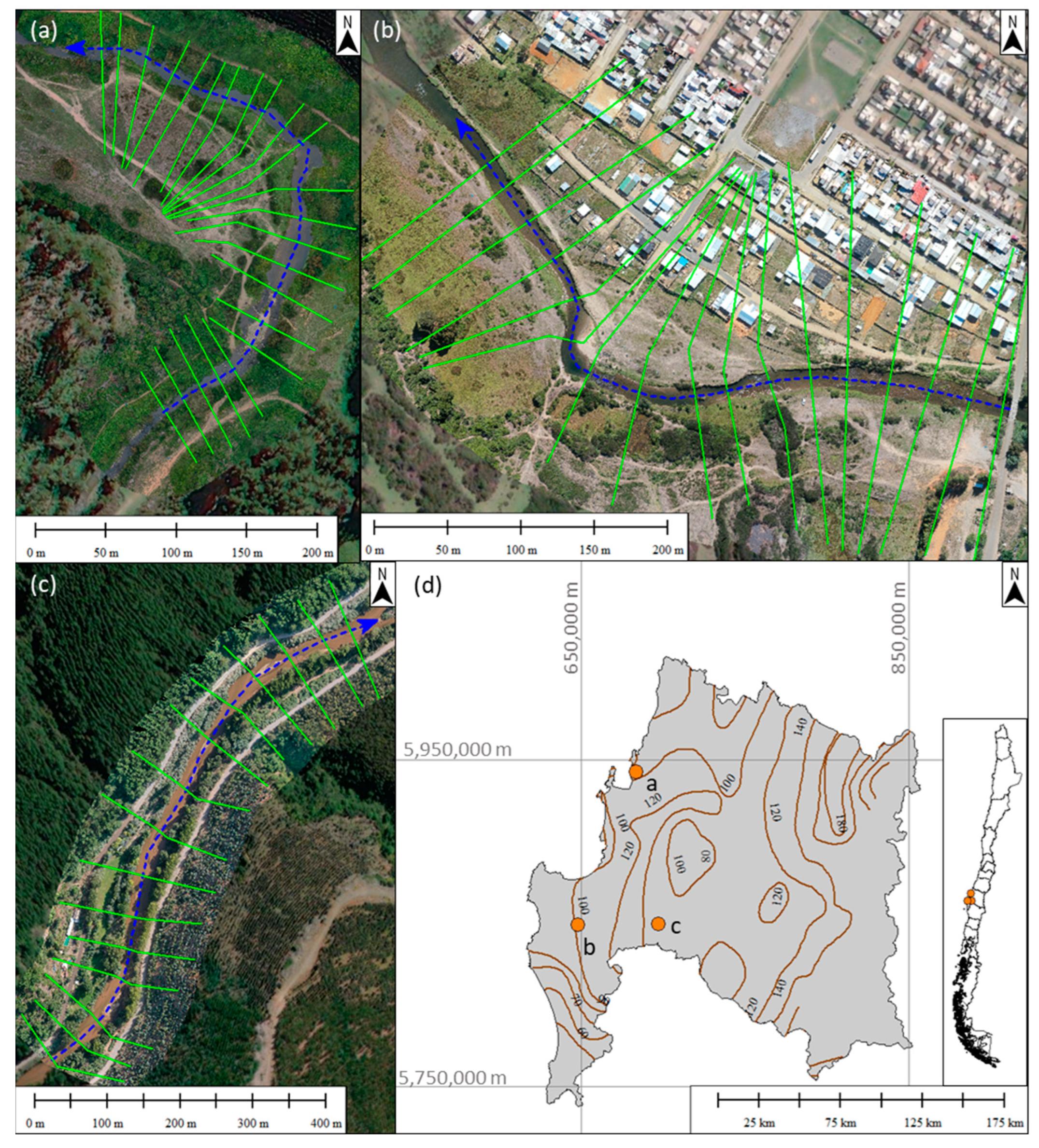
Field campaigns were carried out in the low-water period in three rivers located in south-central Chile (Figure 1). A UAV and RTK-GPS were used to collect topographic and bathymetric information, which was used as a benchmark. For each river, the aero-photogrammetric survey was used along with the bathymetry (RTK-GPS) to generate a traditional DTM (DTM-T). Then, a DTM based on the aero-photogrammetric survey, called the remotely sensed DTM (DTM-RS), was generated, in which the wet part of the river was assumed to have a flat bed.
Based on each DTM, a hydraulic model (HM) was constructed. That is, for each river, two geometries were generated that gave rise to two models: (i) with field data captured using traditional methods, defined as HM-T, and (ii) created using remote sensing data, defined as HM-RS.
For the HM-T and HM-RS of each river to be comparable, 1D steady-state modeling was used, in which the slope of the water surface obtained by means of remote sensing was used as the boundary condition. In addition, Manning’s n, detailed by Chow [59], was used as a roughness parameter, associated with river vegetation and irregularities, and was determined by visual inspection of the orthophoto of each river, from which a representative coefficient of the channel and its floodplain was obtained for flood scenarios. Thus, HM-T was considered as a reference and representative of the channel, and based on this model, comparisons and analysis of the results with respect to HM-RS were performed.
2.1. Study Area
Three sections of the Bellavista, Curanilahue, and Nicodahue rivers, located in south-central Chile (Figure 1), were selected for this study. These rivers have an exclusively pluvial regime, with greater flows during the austral winter months (June to September) and lower flows from January to April. A reference precipitation value for flood estimation is the 24 h maximum annual precipitation for a 10-year return period (P2410), which is 95, 100, and 120 mm for the Bellavista, Curanilahue, and Nicodahue areas, respectively [60].
The topographic surveys were conducted between the months of February and April 2021 (during low-water conditions). Figure 1 shows the Bellavista, Curanilahue, and Nicodahue channels, with their locations in Chile.
2.2. Morphological Channel Classification
For the channel classification and subsequent analysis, the classification system proposed by Rosgen [61] was used. This classification has four levels: basic morphological characterization (level I), morphological description (level II), assessment of river stability conditions (level III), and verification (level IV). The Rosgen classification has been used to understand processes in rivers and their morphology [62] for stream restoration design [63,64], to aid in complex riparian ecological site descriptions [65], and other purposes.
In this study, classification level II was applied, which provides a detailed morphological description of the channel based on information collected in the field. This level of morphological description requires the calculation of the entrenchment ratio (ER), width/depth ratio (W/D), sinuosity, and surface slope, along with the determination of the riverbed material [61].
The entrenchment ratio is defined as the ratio of the width of the channel at a water height associated with a 50-year-return-period flow and the bankfull width. The bankfull flow is that which fills the entire channel section before the floodplain is flooded [66]. According to Rosgen [61], the occurrence interval of this flow is generally 1.5 to 2 years. Meanwhile, the W/D ratio is measured in reference to the bankfull stage [67]. Sinuosity is defined as the quotient of the channel length divided by valley length [61,68]. Water surface slope is determined by measuring the difference in water surface elevation over the length of the channel.
Information collected using remote sensing, along with the Rosgen classification parameters, was used to determine river typology. In the tolerances suggested in the method for river classification, the values for the entrenchment ratio can vary by ±0.2 units and the width/depth ratio can vary by ±2 units as a function of the continuum of physical variables within stream reaches [61].
2.3. Field Measurements
In the field campaign, topographic surveys were carried out using remote sensing and cross sections were plotted with RTK-GPS.
The remote sensing topographic survey was conducted using a four-motor rotary wing Mavic 2 Pro (DJI Technology Co., Ltd., Shenzhen, China) UAV with a 1″ 20 MP sensor. The images captured by the UAV had a longitudinal and lateral overlap of 80%, with a flight elevation of 100 m and a velocity of 25 km/h. In addition, a rolling shutter effect correction was carried out. Each survey was georeferenced, and accuracy was controlled using 5 ground control points (GCP) measured with a differential GPS in RTK mode. The GCP were distributed among the vertices and center of the study area; mean RMS errors of 0.033, 0.023, and 0.015 m were obtained for Bellavista, Curanilahue, and Nicodahue, respectively.
The images captured by the UAV were processed with Pix4D® version 4.5 [69]. Pix4D is software designed for aerial mapping and 3D modeling of large-scale areas and objects using unmanned aerial vehicles (UAVs) [70]. A georeferenced orthophoto was obtained along with a color point cloud with 10 cm spacing in LAZ format for each river. LAZ (LASzip) is a lossless compression format based on the binary file format designed for transmitting point cloud data that is supported by all contemporary LIDAR processing software tools [71]. Based on the differences relative to the local mean, colors, elevations, and the use of orthorectified aerial photography, a semi-automatic classification of the points as terrain or not terrain was carried out. The points classified as terrain were subsequently used to construct the topography of each river.
Meanwhile, to characterize the bathymetry of each channel, cross sections were measured by wading the river from bank to bank; a distance between cross sections of approximately 30 m was used, which increased as a function of channel homogeneity. Thus, the channel bed was represented using RTK-GPS. Based on the bathymetric survey, a DTM of the channel bed was derived using the triangulated irregular network (TIN) method.
2.4. DTM-Traditional (DTM-T) and DTM-Remote Sensing (DTM-RS)
For each river, DTM-T and DTM-RS were constructed. To this end, the boundary between the wet and dry zones of the river was identified via aerial photography; thus, the wet and dry zones were processed independently. The topography was obtained using the point cloud in LAZ format classified as terrain, derived from photographs obtained using the UAV. Meanwhile, the DMT-T bathymetry was characterized through river cross sections using RTK-GPS, while the DTM-RS bathymetry was constructed using the water level obtained from the aerophotogrammetric survey, with identification of points on the channel banks that represent the water surface elevation.
2.5. Flow Discharge Data
Because the sections of the rivers under study are ungauged, the rational method was used to calculate the flood flows for the hydraulic model [72]. The rational method (Equation (1)) is a conceptual model to estimate the maximum flow (Q) at a basin outlet based on rainfall intensity (i), the area of the catchment basin (A), and an empirical factor called the runoff coefficient (C), which depends, among other variables, on the soil type, return period and land cover in the basin [73,74].
Q(T) = C·i(T)·A.
Using the rational method, flows for return periods (T) of T = 2, 5, 10, 25, 50, 100, and 150 years were calculated, with (C) varying according to the analyzed return period and channel location. In the present analysis, this coefficient varies between 0.33 at T = 2 and 0.39 at T = 150 for the studied rivers [75,76]. Meanwhile, rainfall intensity was calculated based on maximum 24 h rainfall, basin time of concentration (Tc), and the drag coefficient (CD). By means of a map of rainfall isohyets [60], the P2410 was obtained for each area; Tc was calculated using the California Culvert Practice formula (1942), designed for small basins, while for the drag coefficient (CD) values proposed by Varas and Sánchez [77] were used.
The parameters used and the flows obtained for the Bellavista, Curanilahue, and Nicodahue rivers are shown in Table 1.
2.6. Hydraulic Modeling
Arc GIS v.10.5 software and the Geo Spatial River Analysis System (HEC-Geo RAS v.10.2) were used to extract the geometric data on the active channel and its floodplain from a DTM. To this end, with the use of the georeferenced orthophoto derived from the UAV, the main channel and the boundary between the active channel and floodplain were identified. In addition, to compare the models, the HM-RS cross sections were projected in the same location as the HM-T cross sections obtained using RTK-GPS.
The HEC-RAS version 5.0.3 [78] software developed by the U.S. Army Corps of Engineers represents the channel and flood plain as a series of cross sections perpendicular to the flow, solving all or some of the Saint-Venant equations, depending on the case study. HEC-RAS was used to model the river geometric information extracted from both DTMs. The modeling in HEC-RAS used a one-dimensional (1D), steady-state approach, as it is effective for predicting the extent of floods for hydraulic design and risk assessment purposes [79,80,81,82].
The roughness coefficient for the channel and flood zone was determined by crossing river dimensions and bed size material obtained from the orthophoto derived from the UAV, with the roughness coefficient recommendations provided by Chow [59] for rivers of varying sizes and roughness. Average values for the riverbed and flood plain were estimated for the three studied rivers. Values of n = 0.035 and 0.15 were estimated for the riverbed and flood plain of the Nicodahue River, respectively, while values of 0.045 and 0.05 were estimated for the riverbed and floodplain of the Curanilahue and Bellavista rivers. The modeled flows correspond to floods for return periods of T = 2, 5, 10, 25, 50, 100, and 150 years.
To analyze HM-RS behavior, HM-T was assumed to be the benchmark. The hydraulic models generated for each river were also assumed to be independent of each other. Thus, for both HM-T and HM-RS the same boundary conditions, Manning’s roughness coefficient, river geometry (active channel and floodplain), topography, cross section locations, and flows were used in order to compare the results based on the differences in bathymetry of each model.
To verify the quality of the water surface elevation (WSE) results of the HM-T (WSE-T) and HM-RS (WSE-RS), two objective functions were used to optimize the analysis (minimize their values): the Root Mean Square Error (RMSE) (Equation (2)) and Mean Absolute Error (MAE) (Equation (3)). WSE-T was used as a reference elevation (assumed as correct) and N is the number of cross sections of each river section. In addition, the Mean Absolute Percentage Error (MAPE) (Equation (4)) was used to compare the percentage variation of the depths, obtained from HM-T and HM-RS. To determine depth, bed elevation from the HM-T was used as a reference, along with the WSE results of each modeling, with the depth from the traditional model (Depth-T) used as a reference.
It is important to point out that DGA [58] guidelines are intended for practitioners and hydraulic flood design. In most, river flood-elevation data do not exist, and, moreover, calibration with low flow might not be valid for floods [83]. Therefore, to tackle this issue, the HM-T was considered as a benchmark. In addition, the HM-T is the model design currently used for practitioners; therefore, comparisons against HM-T might result very informative for flood design and risk management.
3. Results
3.1. DTM-T and DTM-RS Results
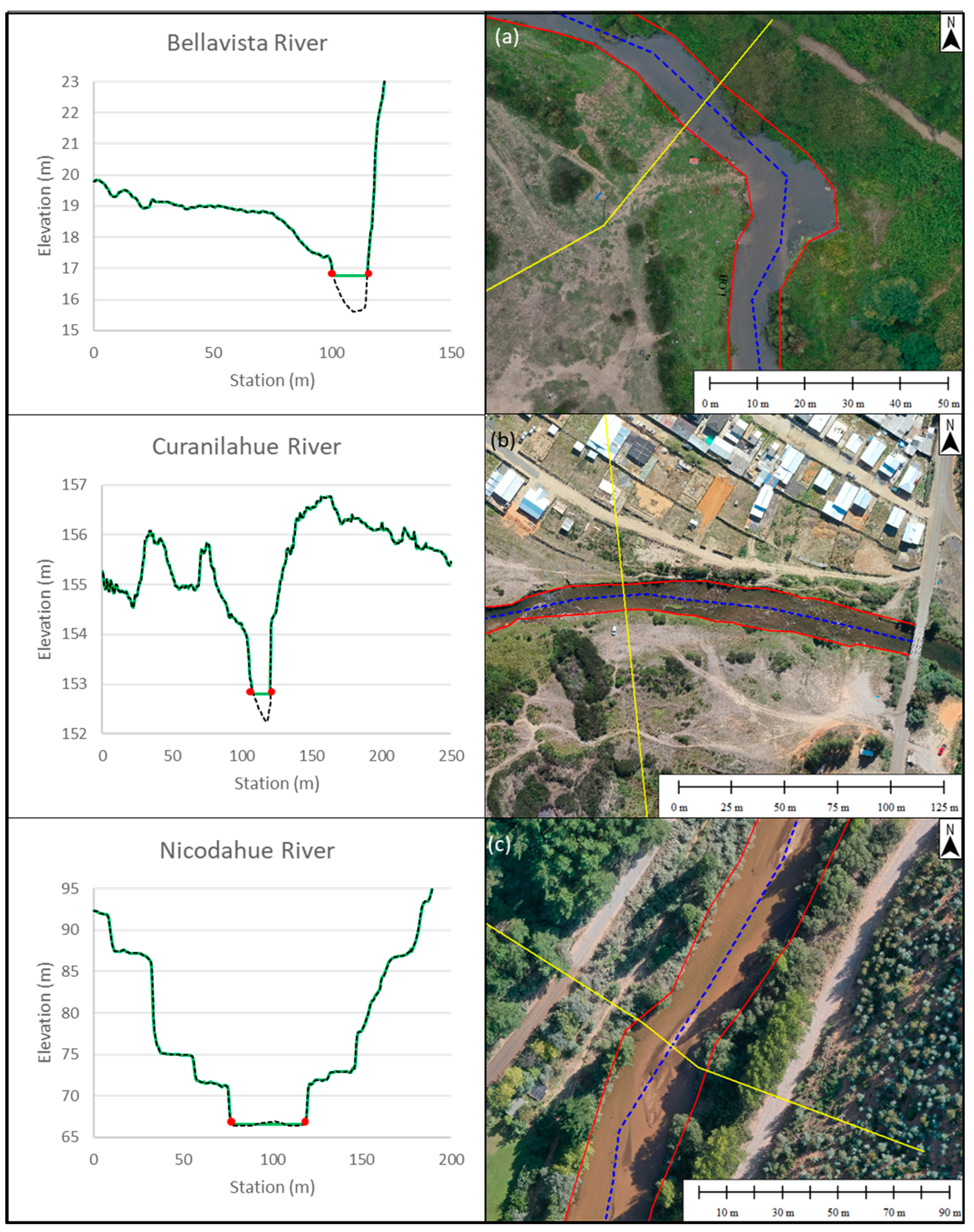
Figure 2 shows, as an example, cross sections and aerial views of the (a) Bellavista, (b) Curanilahue, and (c) Nicodahue rivers. A dotted black line indicates the DTM-T river cross section while the solid green line indicates the cross section derived from the DTM-RS. For the Bellavista and Curanilahue rivers (Figure 2a,b, respectively), the maximum distance differences between the bottom of the channel bed (DTM-T) and the water surface (bottom of the channel bed for the DTM-RS) were 1.13 m and 0.56 m, respectively, and for the Nicodahue River (Figure 2c), this distance was 0.18 m, which is ~3 to 5 times less than that for the Bellavista and Curanilahue rivers.
3.2. Variables for Morphological Description
Table 2 shows the variables of each river section and level II of the Rosgen morphological classification [61], derived from the HM-T results. Figure 3 shows a comparison of the parameters calculated for the description of morphological level II using the HM-T and HM-RS models. Figure 3a shows a comparison between the entrenchment ratio (ER) calculated according to HM-T (ER-T) and ER according to HM-RS (ER-RS) for the Bellavista river for each cross section of the developed model. The dashed blue line indicates the 1:1 ratio of ER-T to ER-RS as a reference. Similarly, Figure 3b shows a comparison of the W/D variable obtained using HM-T and HM-RS (W/D-T and W/D-RS), calculated at the bankfull stage (T = 2 years). Finally, Figure 3c–f show the aforementioned comparisons for the Curanilahue and Nicodahue rivers, respectively.
In addition, maps with the geology of the study sites at watershed scale are included in Figure S1: Maps with the geology of the study sites at watershed scale.
3.3. WSE
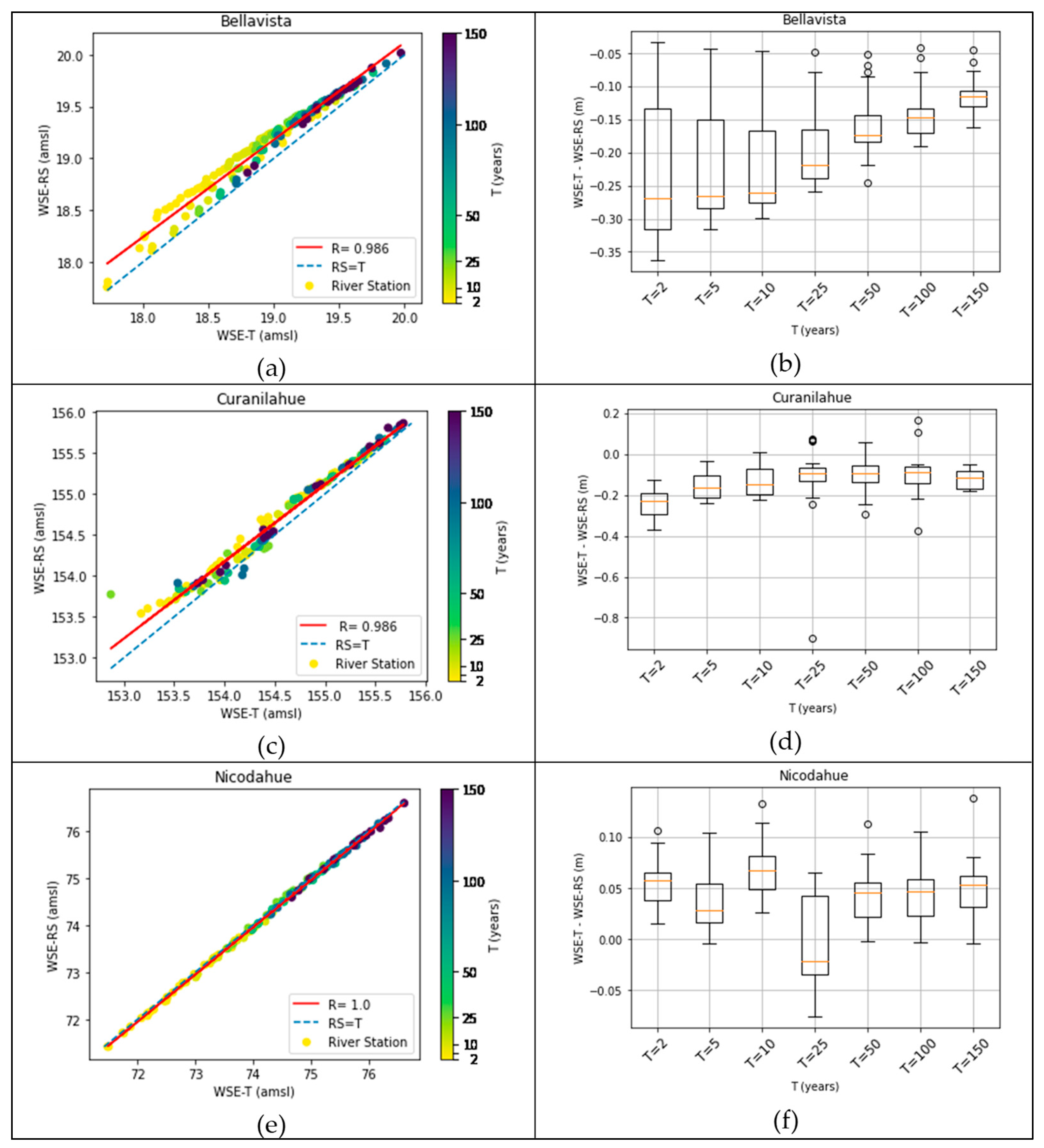
The WSE results for the Bellavista, Curanilahue, and Nicodahue rivers are presented in Figure 4, with Figure 4a,c,e showing a comparison between the WSE-T and WSE-RS results for each cross section of the models at different return periods. The dashed blue line shows the 1:1 ratio of WSE-T to WSE-RS results and the red line shows the trend of the results and their coefficient of correlation®. Figure 4b,d,f show the distribution of the differences between the WSE-T and WSE-RS results of all the cross sections for different return periods.
The minimum and maximum differences for T = 150 in the Bellavista River are −0.7 and −16.2 cm, while in the Curanilahue River they are −0.5 and −17.9 cm. In the Nicodahue River, a high correlation between the WSE results is observed, which suggests small differences between the HM-T and HM-RS results. Thus, the minimum and maximum differences (WSE-T—WSE-RS) in Nicodahue for T = 150 years are −0.4 and 8 cm. For T = 150 years, the mean WSE-T—WSE-RS differences are −11.5, −11.8, and 5.1 cm for Bellavista, Curanilahue, and Nicodahue, respectively.
Table 3 shows the RMSE and MAE results at different return periods for the Bellavista, Curanilahue, and Nicodahue rivers.
Table 3 shows submeter errors, with a trend in Bellavista and Curanilahue of decreasing errors as T increases. The thalweg elevation differences vary between 0.09 and 1.13 m (0.55 m average) in Bellavista and 0.08 and 1.02 m (0.53 m average) in Curanilahue. Both rivers have mostly type C areas according to the Rosgen classification.
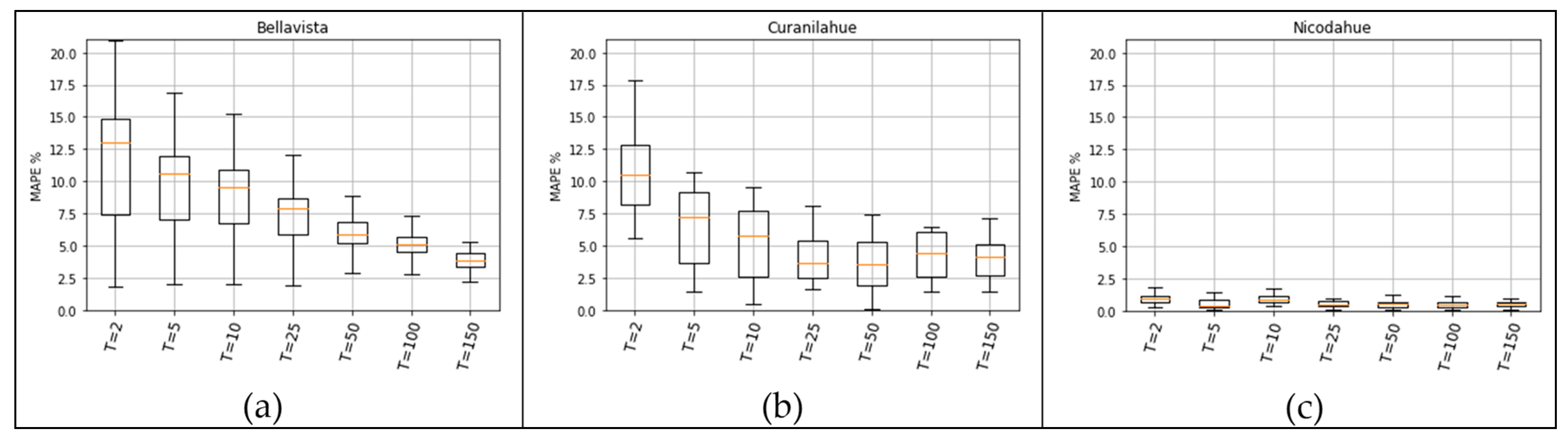
Figure 5 shows, via boxplots, the error percentage variation at different return periods for the Bellavista, Curanilahue, and Nicodahue rivers.
It is observed that for T = 2-year floods, there are MAPE percentage variations of less than 21.0, 17.9, and 1.8% for Bellavista, Curanilahue, and Nicodahue, respectively. The percentage variation decreases as the magnitude of the flood increases. Thus, for a design flow of T = 100, MAPE values below 7.3, 6.4, and 1.1 were obtained for Bellavista, Curanilahue, and Nicodahue, respectively. For a T = 150 flow, a MAPE below 7.1% was obtained for rivers classified as type C, and it was below 1.4% for rivers classified as type B.
The objective function results allow the WSE-RS error to be observed for different floods. This error is associated with the overestimation of WSE-RS, as it is a more conservative result for hydraulic design (T = 100 and 150 years) and overflow risk assessment (T = 2 and 5 years) than WSE-T.
4. Discussion
This study compared two DTMs, one that includes bathymetry obtained using RTK-GPS, called DTM-T, and another that assumes the wet area to have a flat bed, called DTM-RS. For the sake of simplicity in the surveys performed in this study and as RTK-GPS and UAV surveys have nearly the same precision (2 cm for RTK-GPS and 1.5–3.3 cm for the UAV surveys), the dry area (i.e., topography) was derived from UAV measurements. Conducting measurements in the low-water period entails a smaller wet area and therefore reduces the lack of bathymetric information when a flat bed is assumed. Based on each DTM, hydraulic models were constructed that allow a review of morphological variables and estimation of the flood area and WSE.
A flat bed was assumed in the HM-RS bathymetry, which raises the minimum channel elevation and the water surface elevation, which in turn increases the flood width. Thus, it is observed that the W/D-RS results are overestimated with respect to W/D-T for the three studied rivers, which is consistent with expectations. Meanwhile, for ER, different behaviors are observed; in Bellavista, ER-T < ER-RS; in Curanilahue, ER-T > ER-RS; and in Nicodahue, ER-T ≈ ER-RS as the flood widths in HM-RS increase in different proportions relative to the widths obtained from HM-T, which depend on the type of river and its cross section.
According to the Rosgen classification, type B rivers are characterized by having moderate to gentle slopes and narrow valleys that limit the development of a broad floodplain [84]. This classification applies to the Nicodahue River and some sections of the Curanilahue River, where the entrenchment ratio is moderate (1.4–2.2) and W/D > 12. Type C rivers have broad, defined floodplains and in the main channel there are erosion and sediment deposition areas (point bars), with ER > 2.2 and W/D > 12; such characteristics are observed in some sections of the Bellavista and Curanilahue rivers. Type F rivers occur in low areas of valleys, where the channel width increases steadily to a stable, functional floodplain with ER < 1.4 and W/D > 12. The Bellavista River flows in a valley that keeps it entrenched, a type F section, and then changes to type C.
It is observed that in the Bellavista and Nicodahue rivers, the increase in W/D-RS is maintained in the order and distribution of the W/D-T results. In the Nicodahue River, because the floodplain is contained in the valley, the mean variations of W/D and ER are 0.3 and 0.03 m/m, respectively. In Bellavista, W/D-RS increases 2.6 m/m due to the increase in the floodplain area, as does ER-RS, which increases 0.16 m/m on average.
In the Curanilahue River, greater differences are observed, where on average W/D-RS is overestimated by 15.9 m/m with respect to W/D-T. Because it is a slightly entrenched channel, in the HM-RS of Curanilahue, the T = 2 flood occurs above the overflow zone, meaning that the flood width is overestimated. The same effect results in ER-RS values being lower than ER-T, as the differences between flood widths decrease for T = 2 and T = 50 years. Therefore, ER-RS is on average 1.1 m/m less than ER-T. The HM-RS results for Curanilahue suggest an entrenched River (ER < 2.2) with a high W/D-RS ratio, which would lead to an incorrect interpretation for its classification, moving it from class C to class D as an anastomosed river.
While Bellavista and Curanilahue are type C rivers, the differences in W/D ratio and ER behavior are attributed to the type of valley in which they flow. The Bellavista River overflows one of its banks because it borders a colluvial slope along its entire length, while the Curanilahue River floods on both banks.
In the case of slightly entrenched channels (e.g., type C, D, DA, and E), the flows that exceed the bankfull stage overflow their banks and extend to their floodplain, which does not occur in entrenched channels (e.g., type A, F, and G), in which the bank elevations are higher than the bankfull stage. In entrenched channels flows that exceed the bankfull stage increase in depth faster than in width; that is, as channel width increases, the flood area increases only marginally in width [85].
In the Bellavista and Curanilahue rivers, it is observed that WSE-RS tends to be greater than WSE-T; similarly, the distribution of the differences between WSE-T and WSE-RS is mostly negative (WSE-T < WSE-RS). This behavior is expected, as with a flat, higher bathymetry in the DTM-RS, the bottom elevation increases together with WSE. In the Nicodahue River, while the DTM-RS bathymetry is higher than the DTM-T bathymetry, the differences between WSE values are mostly positive (WSE-T > WSE-RS). This behavior is a response to the channel slope, as the upstream flow elevation in the HM-T increases due to the river slope increase, and the effect of the WSE increase remains downstream. Meanwhile, the differences between models are low due to the width and shallow depth of the river, as well as the simplification of channel peculiarities (e.g., islands and sandbanks) of the bathymetry projection in DTM-RS (Figure 2c).
In addition, the decrease in WSE errors is due to the increase in flood width, which compensates for the lack of bathymetric data in the active flood plain using UAVs. Errors are observed to be stable in Nicodahue due to the shallow depth of its initial conditions for the creation of the DTM-RS, the behavior of which at low flows is similar to that at high flows, explained by its degree of lateral confinement. In the Curanilahue river, a slight change in WSE differences trend is observed for the T = 150 years (i.e., the absolute value of the median tends to increase with T, but for T = 150 years, it slightly increases; Figure 4d). This behavior is caused by two cross sections where the HM-RS floods, but the HM-T does not.
A T = 150 year flood is used in various countries [58] for the design and verification of large hydraulic structures. The error results show the overestimation of WSE-RS, making it a more conservative result for hydraulic design. On average, for T = 150 floods, the percentage difference in MAPE is 3.8, 4.2, and 0.55% for Bellavista, Curanilahue, and Nicodahue, respectively. The minor percentage difference is found in river type B.
HM-RS allows flood modeling with conservative results relative to those obtained using HM-T. HM-RS seems to be a safe, low-cost, efficient alternative for developing HM for floods where the WSE is slightly overestimated (up to 15.3 cm of RMSE and 7.3% of depth for T = 100 years) in comparison with the WSE calculated from a HM-T. Therefore, the HM-RS seems to be a recommendable option for practitioners in flood estimation and risk management with a low and controlled overestimation in WSE results.
The approach has important implications in flood studies, as larger areas and cost- and time-efficient flood estimations can be performed using affordable UAVs. Further research in this topic is necessary to estimate the limitations and precision in rivers with different morphologies and under different geographical contexts.
5. Conclusions
This study presented an analysis that explores the utility of a hydraulic flood model derived from remote sensing against a traditional HM used by practitioners in hydraulic engineering. To this end, topographic information obtained using a UAV in low-water periods of wadable rivers was used to construct two digital terrain models for sections of the Bellavista, Curanilahue, and Nicodahue rivers. DTM-T included the bathymetry measured in the field, while in DTM-RS, the bathymetry was assumed to be a flat bed. Based on the DTMs, the hydraulic models HM-T and HM-RS were generated for each river, and the water surface elevation (WSE) behavior was compared, along with the channel morphology and its Rosgen classification.
It was determined that for T = 2-year floods, the MAPE percentage difference in depths is below 21%, and it is greatest for type C rivers. This difference decreases with greater flood magnitudes (greater T) and is below 7.1% in type C rivers and below 1.42% in type B rivers for T = 150-year floods.
Based on the WSE comparison for a T = 150 flood, mean square errors of 0.118, 0.126, and 0.061 m were obtained for Bellavista, Curanilahue, and Nicodahue, which represent mean percentage differences (MAPE) in depth of 3.8, 4.2, and 0.55%, respectively.
In the three modeled rivers, WSE differences tend to decrease as the flow increases. In the Bellavista and Curanilahue rivers, WSE differences are greater with low flows. This is due to the effect of the increase in elevation in the projected DTM-RS bathymetry. This effect decreases with flow increases and in rivers with type C morphology. In type C rivers, flows that overflow the banks increase their width in greater proportion than their depth. Thus, ER and W/D ratios in these rivers cannot be representative. The Nicodahue River, due to its shallow depth in the low-water period, along with its type B morphology (high degree of confinement), presents small differences from T = 2 floods to greater-magnitude floods. The ER and W/D ratios in the Nicodahue River (type B) are representative in HM-RS.
The methodology applied to generate the HM-RS is suitable for shallow channels with a greater dry surface area. The channel morphology classification allows WSE behavior in a flood to be understood, thereby decreasing the uncertainty generated by the area not measured by the UAV. HM-RS allows flood modeling with conservative results relative to those obtained using HM-T, as WSE-RS is overestimated. In addition, in HM-RS, a flat bed is assumed for the bathymetry, which does not involve the collection of information on the wet area of the river, thereby avoiding contact with the river and alteration of the bed. This decreases the risks for the operator when conducting a topographic–bathymetric survey of a river. It also reduces survey-related costs and the times required to obtain results to create a model, making it a recommendable alternative for obtaining a slightly conservative, efficient, economical, and safe approximation for the estimation of floods in rivers in narrow valleys or rivers with defined flood plains.
The current approach represents an exploratory analysis in the right direction for cost- and time-effective flood estimations using UAVs and hydraulic modeling. However, further research in this topic is necessary to validate the main results in broader areas and across rivers with different geomorphology.
Supplementary Materials
The following supporting information can be downloaded at: https://www.mdpi.com/article/10.3390/w15081502/s1, Figure S1: Maps with the geology of the study sites at watershed scale.
Author Contributions
Conceptualization, R.C., E.M., J.L.A., Y.M., D.C. and H.A.; methodology, R.C., E.M. and J.L.A.; software, R.C.; validation, R.C., Y.M., E.M. and J.L.A.; formal analysis, R.C., E.M., J.L.A., Y.M., D.C. and H.A.; investigation, R.C. and E.M.; resources, E.M.; data curation, R.C.; writing—original draft preparation, R.C., E.M., J.L.A., Y.M., D.C. and H.A.; writing—review and editing, R.C., E.M., J.L.A., Y.M., D.C. and H.A.; visualization, R.C. and E.M.; supervision, E.M. and J.L.A.; project administration, E.M.; funding acquisition, E.M. All authors have read and agreed to the published version of the manuscript.
Funding
This research was funded by CIBAS 2019-01 project, DI-FME 03/2021 and by the CRHIAM Center project ANID/FONDAP/15130015.
Data Availability Statement
Publicly available datasets (orthomosaic and digital surface model files) can be found here: [https://www.dropbox.com/sh/t97cuogu9sd7kmq/AAD2IX8haJAgKzSiUCwKSGena?dl=0] (accessed on 1 April 2023).
Acknowledgments
The authors thank Pix4d for proving an educational license for their products and to the CRHIAM Center project ANID/FONDAP/1513001.
Conflicts of Interest
The authors declare no conflict of interest.
References
- Bures, L.; Roub, R.; Sychova, P.; Gdulova, K.; Doubalova, J. Comparison of bathymetric data sources used in hydraulic modelling of floods. Flood Risk Manag. 2018, 12, e12495. [Google Scholar] [CrossRef] [Green Version]
- Wang, X.; Xie, H. A Review on Applications of Remote Sensing and Geographic Information Systems (GIS) in Water Resources and Flood Risk Management. Water 2018, 10, 608. [Google Scholar] [CrossRef] [Green Version]
- Watanabe, Y.; Kawahara, Y. UAV Photogrammetry for Monitoring Changes in River Topography and Vegetation. Procedia Eng. 2016, 154, 317–325. [Google Scholar] [CrossRef] [Green Version]
- Kim, J.S.; Baek, D.; Seo, I.W.; Shin, J. Retrieving shallow stream bathymetry from UAV-assisted RGB imagery using a geospatial regression method. Geomorphology 2019, 341, 102–114. [Google Scholar] [CrossRef]
- McDonald, W. Drones in urban stormwater management: A review and future perspectives. Urban Water J. 2019, 16, 505–518. [Google Scholar] [CrossRef]
- Rosgen, D.L. The Natural Channel Design Method for River Restoration. In Proceedings of the World Environmental and Water Resource Congress, Omaha, Nebraska, 21–25 May 2006; pp. 1–12. [Google Scholar] [CrossRef] [Green Version]
- Degiorgis, M.; Gnecco, G.; Gorni, S.; Roth, G.; Sanguineti, M.; Taramasso, A.C. Classifiers for the detection of flood-prone areas using remote sensed elevation data. J. Hydrol. 2012, 470–471, 302–315. [Google Scholar] [CrossRef]
- Petrović, A.M.; Kovačević-Majkić, J.; Milošević, M.V. Application of run-off model as a contribution to the torrential flood risk management in Topčiderska Reka watershed, Serbia. Nat. Hazards 2016, 82, 1743–1753. [Google Scholar] [CrossRef]
- Salmoral, G.; Casado, M.R.; Muthusamy, M.; Butler, D.; Menon, P.P.; Leinster, P. Guidelines for the use of unmanned aerial systems in flood emergency response. Water 2020, 12, 521. [Google Scholar] [CrossRef] [Green Version]
- Castellarin, A.; Domeneghetti, A.; Brath, A. Identifying robust large-scale flood risk mitigation strategies: A quasi-2D hydraulic model as a tool for the Po river. Phys. Chem. Earth Parts A/B/C 2011, 36, 299–308. [Google Scholar] [CrossRef]
- Koc, K.; Isik, Z. A multi-agent-based model for sustainable governance of urban flood risk mitigation measures. Nat. Hazards 2020, 104, 1079–1110. [Google Scholar] [CrossRef]
- Pandjaitan, N.H.; Sutoyo, S.; Rau, M.I.; Febrita, J.; Dharmawan, I.; Akhmat, I. Comparison between DSM and DTM from photogrammetric UAV in Ngantru Hemlet, Sekaran Village, Bojonegoro East Java. Proc. SPIE 2019, 11372, 678–683. [Google Scholar] [CrossRef]
- Novak, P.; Guinot, V.; Jeffrey, A.; Reeve, D.E. Hydraulic Modelling–An Introduction: Principles, Methods and Applications; CRC Press: Boca Raton, FL, USA, 2018. [Google Scholar]
- Pasquier, U.; He, Y.; Hooton, S.; Goulden, M.; Hiscock, K.M. An integrated 1D-2D hydraulic modelling approach to assess the sensitivity of a coastal region to compound flooding hazard under climate change. Nat. Hazards 2018, 98, 915–937. [Google Scholar] [CrossRef] [Green Version]
- Michaelis, T.; Brandimarte, L.; Mazzoleni, M.; Archfield, S.; Pande, S. Capturing flood-risk dynamics with a coupled agent-based and hydraulic modelling framework. Hydrol. Sci. J. 2020, 65, 1458–1473. [Google Scholar] [CrossRef]
- Quesada-Román, A.; Ballesteros-Cánovas, J.A.; Granados-Bolaños, S.; Birkel, C.; Stoffel, M. Dendrogeomorphic reconstruction of floods in a dynamic tropical river. Geomorphology 2020, 359, 107133. [Google Scholar] [CrossRef]
- Asaad, B.I.; Abed, B.S. Flow Characteristics Of Tigris River Within Baghdad City During Drought. J. Eng. 2020, 26, 77–92. [Google Scholar] [CrossRef] [Green Version]
- Sedighkia, M.; Abdoli, A. Optimizing environmental flow regime by integrating river and reservoir ecosystems. Water Resour. Manag. 2022, 36, 2079–2094. [Google Scholar] [CrossRef]
- Lamouroux, N.; Capra, H.; Pouilly, M. Predicting habitat suitability for lotic fish: Linking statistical hydraulic models with multivariate habitat use models. Regul. Rivers Res. Manag. 1998, 14, 1–11. [Google Scholar] [CrossRef]
- Sundt, H.; Alfredsen, K.; Museth, J.; Forseth, T. Combining green LiDAR bathymetry, aerial images and telemetry data to derive mesoscale habitat characteristics for European grayling and brown trout in a Norwegian river. Hydrobiologia 2022, 849, 509–525. [Google Scholar] [CrossRef]
- Papaioannou, G.; Loukas, A.; Vasiliades, L.; Aronica, G.T.; Gr, G. Flood inundation mapping sensitivity to riverine spatial resolution and modelling approach. Nat. Hazards 2016, 83, 117–132. [Google Scholar] [CrossRef]
- Flener, C.; Lotsari, E.; Alho, P.; Käyhkö, J. Comparison of empirical and theoretical remote sensing based bathymetry models in river environments. River Res. Appl. 2012, 28, 118–133. [Google Scholar] [CrossRef]
- Jawak, S.D.; Vadlamani, S.S.; Luis, A.J.; Jawak, S.D.; Vadlamani, S.S.; Luis, A.J. A Synoptic Review on Deriving Bathymetry Information Using Remote Sensing Technologies: Models, Methods and Comparisons. Adv. Remote Sens. 2015, 4, 147–162. [Google Scholar] [CrossRef] [Green Version]
- Ballesteros Cánovas, J.A.; Eguibar, M.; Bodoque, J.M.; Díez-Herrero, A.; Stoffel, M.; Gutiérrez-Pérez, I. Estimating flash flood discharge in an ungauged mountain catchment with 2D hydraulic models and dendrogeomorphic palaeostage indicators. Hydrol. Process. 2011, 25, 970–979. [Google Scholar] [CrossRef] [Green Version]
- Bodoque, J.M.; Díez-Herrero, A.; Eguibar, M.A.; Benito, G.; Ruiz-Villanueva, V.; Ballesteros-Cánovas, J.A. Challenges in paleoflood hydrology applied to risk analysis in mountainous watersheds—A review. J. Hydrol. 2015, 529, 449–467. [Google Scholar] [CrossRef] [Green Version]
- Koutalakis, P.; Tzoraki, O.; Zaimes, G. drones UAVs for Hydrologic Scopes: Application of a Low-Cost UAV to Estimate Surface Water Velocity by Using Three Different Image-Based Methods. Drones 2019, 3, 14. [Google Scholar] [CrossRef] [Green Version]
- Hill, D.J.; Pypker, T.G.; Church, J. Applications of Unpiloted Aerial Vehicles (UAVs) in Forest Hydrology BT—Forest-Water Interactions; Levia, D.F., Carlyle-Moses, D.E., Iida, S., Michalzik, B., Nanko, K., Tischer, A., Eds.; Springer International Publishing: Cham, Switzerland, 2020; pp. 55–85. [Google Scholar]
- Mazzoleni, M.; Paron, P.; Reali, A.; Juizo, D.; Manane, J.; Brandimarte, L. Testing UAV-derived topography for hydraulic modelling in a tropical environmentderived topography LiDAR RTK-GPS SRTM Hydraulic model Tropical environment. Nat. Hazards 2020, 103, 139–163. [Google Scholar] [CrossRef]
- Granados-Bolaños, S.; Quesada-Román, A.; Alvarado, G.E. Low-cost UAV applications in dynamic tropical volcanic landforms. J. Volcanol. Geotherm. Res. 2021, 410, 107143. [Google Scholar] [CrossRef]
- Zhao, C.; Zhang, C.; Yang, S.; Liu, C.; Xiang, H.; Sun, Y.; Yang, Z.; Zhang, Y.; Yu, X.; Shao, N.; et al. Calculating e-flow using UAV and ground monitoring. J. Hydrol. 2017, 552, 351–365. [Google Scholar] [CrossRef]
- Carbonneau, P.E.; Dietrich, J.T. Cost-effective non-metric photogrammetry from consumer-grade sUAS: Implications for direct georeferencing of structure from motion photogrammetry. Earth Surf. Process. Landf. 2016, 42, 473–486. [Google Scholar] [CrossRef] [Green Version]
- Santise, M.; Fornari, M.; Forlani, G.; Roncella, R. Evaluation of dem generation accuracy from uas imagery. Int. Arch. Photogramm. Remote Sens. Spat. Inf. Sci. 2014, 45, 529–536. [Google Scholar] [CrossRef] [Green Version]
- Bandini, F.; Sunding, T.P.; Linde, J.; Smith, O.; Jensen, I.K.; Köppl, C.J.; Butts, M.; Bauer-Gottwein, P. Unmanned Aerial System (UAS) observations of water surface elevation in a small stream: Comparison of radar altimetry, LIDAR and photogrammetry techniques. Remote Sens. Environ. 2020, 237, 111487. [Google Scholar] [CrossRef]
- King, T.V.; Neilson, B.T.; Rasmussen, M.T. Estimating Discharge in Low-Order Rivers With High-Resolution Aerial Imagery. Water Resour. Res. 2018, 54, 863–878. [Google Scholar] [CrossRef] [Green Version]
- Hicks, D.M. Remotely Sensed Topographic Change in Gravel Riverbeds with Flowing Channels. In Gravel—Bed Rivers; John Wiley & Sons, Ltd.: Hoboken, NJ, USA, 2012; pp. 303–314. [Google Scholar]
- Williams, R.D.; Brasington, J.; Vericat, D.; Hicks, D.M. Hyperscale terrain modelling of braided rivers: Fusing mobile terrestrial laser scanning and optical bathymetric mapping. Earth Surf. Process. Landf. 2014, 39, 167–183. [Google Scholar] [CrossRef]
- Flener, C.; Vaaja, M.; Jaakkola, A.; Krooks, A.; Kaartinen, H.; Kukko, A.; Kasvi, E.; Hyyppä, H.; Hyyppä, J.; Alho, P. Seamless mapping of river channels at high resolution using mobile LiDAR and UAV-photography. Remote Sens. 2013, 5, 6382–6407. [Google Scholar] [CrossRef] [Green Version]
- Brasington, J.; Rumsby, B.T.; McVey, R.A. Monitoring and modelling morphological change in a braided gravel-bed river using high resolution GPS-based survey. Earth Surf. Process. Landf. 2000, 25, 973–990. [Google Scholar] [CrossRef]
- Lane, S.N.; Richards, K.S.; Chandler, J.H. Developments in monitoring and modelling small-scale river bed topography. Earth Surf. Process. Landf. 1994, 19, 349–368. [Google Scholar] [CrossRef]
- Milne, J.A.; Sear, D.A. Modelling river channel topography using GIS. Int. J. Geogr. Inf. Sci. 1997, 11, 499–519. [Google Scholar] [CrossRef]
- Koljonen, S.; Huusko, A.; Mäki-Petäys, A.; Louhi, P.; Muotka, T. Assessing Habitat Suitability for Juvenile Atlantic Salmon in Relation to In-Stream Restoration and Discharge Variability. Restor. Ecol. 2013, 21, 344–352. [Google Scholar] [CrossRef]
- Kinzel, P.J.; Legleiter, C.J.; Nelson, J.M. Mapping River Bathymetry With a Small Footprint Green LiDAR: Applications and Challenges1. JAWRA J. Am. Water Resour. Assoc. 2013, 49, 183–204. [Google Scholar] [CrossRef]
- Guenther, G.C. Airborne lidar bathymetry. Digit. Elev. Model Technol. Appl. DEM Users Man. 2007, 2, 253–320. [Google Scholar]
- Guerrero, M.; Lamberti, A. Flow field and morphology mapping using ADCP and multibeam techniques: Survey in the Po River. J. Hydraul. Eng. 2011, 137, 1576–1587. [Google Scholar] [CrossRef]
- Kasvi, E.; Laamanen, L.; Lotsari, E.; Alho, P. Flow Patterns and Morphological Changes in a Sandy Meander Bend during a Flood—Spatially and Temporally Intensive ADCP Measurement Approach. Water 2017, 9, 106. [Google Scholar] [CrossRef] [Green Version]
- Westaway, R.M.; Lane, S.N.; Hicks, D.M. Remote sensing of clear-water, shallow, gravel-bed rivers using digital photogrammetry. Photogramm. Eng. Remote Sens. 2001, 67, 1271–1282. [Google Scholar]
- Kasvi, E.; Salmela, J.; Lotsari, E.; Kumpula, T.; Lane, S.N. Comparison of remote sensing based approaches for mapping bathymetry of shallow, clear water rivers. Geomorphology 2019, 333, 180–197. [Google Scholar] [CrossRef]
- Billard, B.; Abbot, R.H.; Penny, M.F. Airborne estimation of sea turbidity parameters from the WRELADS laser airborne depth sounder. Appl. Opt. 1986, 25, 2080–2088. [Google Scholar] [CrossRef] [PubMed]
- Eren, F.; Pe’eri, S.; Rzhanov, Y.; Ward, L. Bottom characterization by using airborne lidar bathymetry (ALB) waveform features obtained from bottom return residual analysis. Remote Sens. Environ. 2018, 206, 260–274. [Google Scholar] [CrossRef]
- Hilldale, R.C.; Raff, D. Assessing the ability of airborne LiDAR to map river bathymetry. Earth Surf. Process. Landf. 2008, 33, 773–783. [Google Scholar] [CrossRef]
- Lin, Y.-C.; Cheng, Y.-T.; Zhou, T.; Ravi, R.; Hasheminasab, S.M.; Flatt, J.E.; Troy, C.; Habib, A. Evaluation of UAV LiDAR for Mapping Coastal Environments. Remote Sens. 2019, 11, 2893. [Google Scholar] [CrossRef] [Green Version]
- Hilldale, R.C. Using Bathymetric LiDAR and a 2-D Hydraulic Model to Identify Aquatic River Habitat. In Proceedings of the World Environmental and Water Resources Congress 2007: Restoring Our Natural Habitat, Tampa, FL, USA, 15–19 May 2007; pp. 1–18. [Google Scholar]
- Mihu-Pintilie, A.; Cîmpianu, C.I.; Stoleriu, C.C.; Pérez, M.N.; Paveluc, L.E. Using High-Density LiDAR Data and 2D Streamflow Hydraulic Modeling to Improve Urban Flood Hazard Maps: A HEC-RAS Multi-Scenario Approach. Water 2019, 11, 1832. [Google Scholar] [CrossRef] [Green Version]
- Costa, B.M.; Battista, T.A.; Pittman, S.J. Comparative evaluation of airborne LiDAR and ship-based multibeam SoNAR bathymetry and intensity for mapping coral reef ecosystems. Remote Sens. Environ. 2009, 113, 1082–1100. [Google Scholar] [CrossRef]
- Genchi, S.A.; Vitale, A.J.; Perillo, G.M.E.; Seitz, C.; Delrieux, C.A. Mapping Topobathymetry in a Shallow Tidal Environment Using Low-Cost Technology. Remote Sens. 2020, 12, 1394. [Google Scholar] [CrossRef]
- Lei, T.; Wang, J.; Li, X.; Wang, W.; Shao, C.; Liu, B. Flood Disaster Monitoring and Emergency Assessment Based on Multi-Source Remote Sensing Observations. Water 2022, 14, 2207. [Google Scholar] [CrossRef]
- Jiménez-Jiménez, S.; Ojeda, W.; Marcial, M.D.; Enciso, J. Digital Terrain Models Generated with Low-Cost UAV Photogrammetry: Methodology and Accuracy. ISPRS Int. J. Geo-Inf. 2021, 10, 285. [Google Scholar] [CrossRef]
- DGA. Guías Metodológicas Para Presentación y Revisión Técnica de Proyectos de Modificación de Cauces Naturales Y Artificiales; DGA: Santiago, Chile, 2016. [Google Scholar]
- Chow, V.T. Open-Channel Hydraulics, Classical Textbook Reissue; McGraw-Hill: New York, NY, USA, 1988. [Google Scholar]
- DGA. Precipitaciones Máximas Diarias (Mapoteca Digital). 2018. Available online: https://dga.mop.gob.cl (accessed on 15 January 2023).
- Rosgen, D.L. A classification of natural rivers. Catena 1994, 22, 169–199. [Google Scholar] [CrossRef] [Green Version]
- Rajabi, M.; Roostaei, S.; Barzkar, M. Morphological classification stability of Zab river channel on Rosgen method. Geogr. Plan. 2021, 25, 141–155. [Google Scholar] [CrossRef]
- Schwartz, J.S. Use of Ecohydraulic-Based Mesohabitat Classification and Fish Species Traits for Stream Restoration Design. Water 2016, 8, 520. [Google Scholar] [CrossRef] [Green Version]
- Rosgen, D.L. Rosgen, D.L. Rosgen geomorphic channel design. In Part 654 Stream Restoration Design National Engineering Handbook; United States Department of Agriculture: Washington, DC, USA, 2007. [Google Scholar]
- Meehan, M.A.; O’Brien, P.L. Using the Rosgen Stream Classification System to Aid in Riparian Complex Ecological Site Descriptions Development. Rangel. Ecol. Manag. 2019, 72, 729–735. [Google Scholar] [CrossRef]
- Wolman, M.G.; Leopold, L.B. River Flood Plains: Some Observations on Their Formation; US Government Printing Office: Washington, DC, USA, 1957. [Google Scholar]
- Williams, G.P. Bank-full discharge of rivers. Water Resour. Res. 1978, 14, 1141–1154. [Google Scholar] [CrossRef]
- Friend, P.F.; Sinha, R. Braiding and meandering parameters. Geol. Soc. Lond. Spec. Publ. 1993, 75, 105–111. [Google Scholar] [CrossRef]
- Becker, C.; Häni, N.; Rosinskaya, E.; d’Angelo, E.; Strecha, C. Classification of aerial photogrammetric 3D point clouds. arXiv 2017, arXiv:1705.08374. [Google Scholar] [CrossRef] [Green Version]
- Walter, J.; Edwards, J.; McDonald, G.; Kuchel, H. Photogrammetry for the estimation of wheat biomass and harvest index. Field Crop. Res. 2018, 216, 165–174. [Google Scholar] [CrossRef]
- Deems, J.S.; Painter, T.H.; Finnegan, D.C. Lidar measurement of snow depth: A review. J. Glaciol. 2013, 59, 467–479. [Google Scholar] [CrossRef] [Green Version]
- Schaake, J.C., Jr.; Geyer, J.C.; Knapp, J.W. Experimental examination of the rational method. J. Hydraul. Div. 1967, 93, 353–370. [Google Scholar] [CrossRef]
- Mulvaney, T.J. On the use of self-registering rain and flood gauges in making observations of the relations of rainfall and flood discharges in a given catchment. Proc. Inst. Civ. Eng. Irel. 1851, 4, 19–31. [Google Scholar]
- Campos, J.N.B.; Studart, T.M.; Souza Filho, D.F.; Porto, V.C. On the Rainfall Intensity–Duration–Frequency Curves, Partial-Area Effect and the Rational Method: Theory and the Engineering Practice. Water 2020, 12, 2730. [Google Scholar] [CrossRef]
- Ayala, C.; Vidal Jara, F.; Ayala Riquelme, L. Manual de Cálculo de Crecidas y Caudales Mínimos en Cuencas sin Información Fluviométrica. Ministerio de Obras Públicas, Dirección General de Aguas: Santiago, Chile, 1995. Agosto. Available online: https://snia.mop.gob.cl/sad/FLU398.pdf (accessed on 15 January 2023).
- MOP. Manual de Carreteras Volumen N° 2. Procedimientos de Estudios Viales. 2022. Available online: https://mc.mop.gob.cl (accessed on 15 January 2023).
- Varas, E.; Sánchez, S. Curvas Generalizadas de Intensidad-Duración-Frecuencia de Lluvias. Hidrol. Dren. Vial. Chile 1988. Available online: http://www.dga.cl/estudiospublicaciones/mapoteca/Balance%20Hdrico/isoyetas.zip (accessed on 15 January 2023).
- Charley, W.J. The Hydrologic Modeling System (HEC-HMS): Design and Development Issues; US Army Corps of Engineers, Hydrologic Engineering Center: Davis, CA, USA, 1995. [Google Scholar]
- Horritt, M.S.; Bates, P.D. Evaluation of 1D and 2D numerical models for predicting river flood inundation. J. Hydrol. 2002, 268, 87–99. [Google Scholar] [CrossRef]
- Lamichhane, N.; Sharma, S. Development of Flood Warning System and Flood Inundation Mapping Using Field Survey and LiDAR Data for the Grand River near the City of Painesville, Ohio. Hydrology 2017, 4, 24. [Google Scholar] [CrossRef] [Green Version]
- Namara, W.G.; Damisse, T.A.; Tufa, F.G. Application of HEC-RAS and HEC-GeoRAS model for Flood Inundation Mapping, the case of Awash Bello Flood Plain, Upper Awash River Basin, Oromiya Regional State, Ethiopia. Model. Earth Syst. Environ. 2021, 8, 1449–1460. [Google Scholar] [CrossRef]
- Quesada-Román, A.; Ballesteros-Cánovas, J.A.; Granados-Bolaños, S.; Birkel, C.; Stoffel, M. Improving regional flood risk assessment using flood frequency and dendrogeomorphic analyses in mountain catchments impacted by tropical cyclones. Geomorphology 2022, 396, 108000. [Google Scholar] [CrossRef]
- Azamathulla, H.M.; Jarrett, R.D. Use of Gene-Expression Programming to Estimate Manning’s Roughness Coefficient for High Gradient Streams. Water Resour. Manag. 2013, 27, 715–729. [Google Scholar] [CrossRef]
- Haile, A.T.; Asfaw, W.; Rientjes, T.; Worako, A.W. Deterioration of streamflow monitoring in Omo-Gibe basin in Ethiopia. Hydrol. Sci. J. 2022, 67, 1040–1053. [Google Scholar] [CrossRef]
- Rosgen, D.L. Applied River Morphology; Wildland Hydrology: Pagosa Springs, CO, USA, 1996. [Google Scholar]
Figure 1.
Orthophoto of the (a) Bellavista (Lat/Lon: 36°38′51″ S, 72°56′41″ W), (b) Curanilahue (Lat/Lon: 37°29′35″ S, 73°19′21″ W), and (c) Nicodahue (Lat/Lon: 37°29′13″ S, 72°46′25″ W) rivers and (d) their locations in Chile, with a map of rainfall isohyets in mm. The green lines indicate the cross sections of the modeling domain and the blue lines indicate the flow directions of the rivers. Coordinates UTM 18S (WGS 84).

Figure 2.
Cross sections of the (a) Bellavista (Lat/Lon: 37°29′34″ S, 73°19′27″ W), (b) Curanilahue (Lat/Lon: 37°29′34″ S, 73°19′27″ W), and (c) Nicodahue (Lat/Lon: 37°29′04″ S, 72°46′21″ W) rivers. The solid line shows the flat bed assumed using the DTM-RS, while the dotted line is from the DTM-T. The right panels show an aerial view of the river, while the left panels show the cross section (yellow line) derived for the DTM-RS and DTM-T. The red lines indicate the banks.

Figure 3.
Comparison of entrenchment ratio (ER-T vs. ER-RS) and comparison of width/depth ratio (W/D-T vs. W/D-RS) for the Bellavista (a,b), Curanilahue (c,d), and Nicodahue rivers (e,f). The dashed blue line represents the 1:1 ratio of the RS to T results. R2 as the coefficient of determination.
Figure 3.
Comparison of entrenchment ratio (ER-T vs. ER-RS) and comparison of width/depth ratio (W/D-T vs. W/D-RS) for the Bellavista (a,b), Curanilahue (c,d), and Nicodahue rivers (e,f). The dashed blue line represents the 1:1 ratio of the RS to T results. R2 as the coefficient of determination.

Figure 4.
WSE-RS vs. WSE-T results for each cross section of the (a) Bellavista, (c) Curanilahue, and (e) Nicodahue rivers for different return periods. The dashed blue line shows the 1:1 ratio of WSE-T to WSR-RS and the red line shows the trend of the results and correlation (R). (b,d,f) show the distribution of differences between WSE-T and WSE-RS for the Bellavista, Curanilahue, and Nicodahue rivers, respectively.

Figure 5.
Boxplots of the absolute percentage differences in depth between HM-T and HM-RS at different return periods for the (a) Bellavista, (b) Curanilahue, and (c) Nicodahue rivers.
Figure 5.
Boxplots of the absolute percentage differences in depth between HM-T and HM-RS at different return periods for the (a) Bellavista, (b) Curanilahue, and (c) Nicodahue rivers.


Table 1.
Parameters and flows calculated using the rational method for different return periods for the Bellavista, Curanilahue, and Nicodahue rivers.
Table 1.
Parameters and flows calculated using the rational method for different return periods for the Bellavista, Curanilahue, and Nicodahue rivers.
| River | A (km2) | Tc (hr) | CD | Q(m3/s) | |||||||
|---|---|---|---|---|---|---|---|---|---|---|---|
| T = 2 | T = 5 | T = 10 | T = 25 | T = 50 | T = 100 | T = 150 | |||||
| Bellavista | 81.9 | 4.05 | 0.38 | 95 | 46.5 | 64.3 | 73.8 | 85.3 | 95.8 | 103.9 | 113.2 |
| Curanilahue | 70.9 | 2.06 | 0.28 | 100 | 64.2 | 86.3 | 97.4 | 109.4 | 116.5 | 131.9 | 140.4 |
| Nicodahue | 727.6 | 5.11 | 0.43 | 120 | 468.6 | 648.2 | 744.1 | 860.2 | 965.7 | 1048 | 1141.3 |
Table 2.
Morphological characteristics of the studied river sections.
| River | Bellavista | Curanilahue | Nicodahue |
|---|---|---|---|
| Sinuosity | 1.522 | 1.172 | 1.056 |
| Slope | 0.0039 | 0.0034 | 0.0015 |
| Channel material | Cobble | Cobble | Gravel |
| Length (m) | 391 | 455 | 755 |
| Date measured | 16-02-2021 | 25-03-2021 | 18-03-2021 |
| Rosgen Classification | F3; C3 | B3c; C3 | B4c |
Table 3.
Objective functions (O.F.), Root Mean Square Error (RMSE) and Mean Absolute Error (MAE) values for the WSE comparison at different return periods for the Bellavista, Curanilahue, and Nicodahue rivers.
Table 3.
Objective functions (O.F.), Root Mean Square Error (RMSE) and Mean Absolute Error (MAE) values for the WSE comparison at different return periods for the Bellavista, Curanilahue, and Nicodahue rivers.
| River | O.F. | T = 2 | T = 5 | T = 10 | T = 25 | T = 50 | T = 100 | T = 150 |
|---|---|---|---|---|---|---|---|---|
| Bellavista | RMSE (m) | 0.251 | 0.233 | 0.228 | 0.201 | 0.167 | 0.148 | 0.118 |
| MAE (m) | 0.230 | 0.218 | 0.214 | 0.191 | 0.159 | 0.142 | 0.115 | |
| Curanilahue | RMSE (m) | 0.251 | 0.171 | 0.149 | 0.250 | 0.137 | 0.153 | 0.126 |
| MAE (m) | 0.240 | 0.156 | 0.132 | 0.158 | 0.112 | 0.131 | 0.118 | |
| Nicodahue | RMSE (m) | 0.060 | 0.047 | 0.076 | 0.045 | 0.054 | 0.054 | 0.061 |
| MAE (m) | 0.055 | 0.038 | 0.070 | 0.041 | 0.045 | 0.047 | 0.052 |
Disclaimer/Publisher’s Note: The statements, opinions and data contained in all publications are solely those of the individual author(s) and contributor(s) and not of MDPI and/or the editor(s). MDPI and/or the editor(s) disclaim responsibility for any injury to people or property resulting from any ideas, methods, instructions or products referred to in the content. |
© 2023 by the authors. Licensee MDPI, Basel, Switzerland. This article is an open access article distributed under the terms and conditions of the Creative Commons Attribution (CC BY) license (https://creativecommons.org/licenses/by/4.0/).
Share and Cite
MDPI and ACS Style
Clasing, R.; Muñoz, E.; Arumí, J.L.; Caamaño, D.; Alcayaga, H.; Medina, Y. Remote Sensing with UAVs for Modeling Floods: An Exploratory Approach Based on Three Chilean Rivers. Water 2023, 15, 1502. https://doi.org/10.3390/w15081502
AMA Style
Clasing R, Muñoz E, Arumí JL, Caamaño D, Alcayaga H, Medina Y. Remote Sensing with UAVs for Modeling Floods: An Exploratory Approach Based on Three Chilean Rivers. Water. 2023; 15(8):1502. https://doi.org/10.3390/w15081502
Chicago/Turabian StyleClasing, Robert, Enrique Muñoz, José Luis Arumí, Diego Caamaño, Hernán Alcayaga, and Yelena Medina. 2023. "Remote Sensing with UAVs for Modeling Floods: An Exploratory Approach Based on Three Chilean Rivers" Water 15, no. 8: 1502. https://doi.org/10.3390/w15081502
Note that from the first issue of 2016, this journal uses article numbers instead of page numbers. See further details here.