

A Comparison of Different Methods for Modelling Water Hammer Valve Closure with CFD

1
Department of Engineering Sciences and Mathematics, Luleå University of Technology, 971 87 Luleå, Sweden
2
Department of Hydraulics, Hydraulic Machinery and Environmental Engineering, University Politehnica of Bucharest, 060042 București, Romania
3
Vattenfall AB, 162 87 Stockholm, Sweden
*
Author to whom correspondence should be addressed.
Water 2023, 15(8), 1510; https://doi.org/10.3390/w15081510
Submission received: 10 March 2023
/
Revised: 4 April 2023
/
Accepted: 10 April 2023
/
Published: 12 April 2023
(This article belongs to the Special Issue About an Important Phenomenon—Water Hammer)
Abstract
:Water hammer is a transient phenomenon that occurs when a flowing fluid is rapidly decelerated, which can be harmful and damaging to a piping system. Three-dimensional computational fluid dynamics (CFD) with three-dimensional geometry is a common tool for studying water hammer, which is more accurate than numerical simulation with one-dimension approximation of the geometry. There are different methods with different accuracy and computational costs for valve closure modelling. This paper presents the result of water hammer 3D simulation with three main technics for modelling an axial valve closure: dynamic mesh, sliding mesh, and immersed solid methods. The variation of the differential pressure variation and the wall shear stress are compared with experimental results. Additionally, the 3D effects of the flow after the valve closure and the computational cost are addressed. The sliding mesh method presents the most physical results compared to the other two methods. The immersed solid method predicts a smaller pressure rise which may be the result of using a source term in the momentum equation instead of modelling the valve movement. The dynamic mesh method adds fluctuations to the primary phenomenon. Moreover, the sliding mesh is less expensive than the dynamic mesh method in terms of computational cost (approximately one-third), which was the primary method for axial valve closure modelling in the literature.
1. Introduction
Water hammer is a transient phenomenon caused by a sudden deceleration of the water in a closed system. Water hammer may cause a considerable pressure spike, just after the deceleration or acceleration of the fluid, followed by a pressure wave that travels periodically along the pipe. The wave is damped as it travels back and forth along the pipe. Water hammer may create strong vibrations, which put piping and equipment such as pumps and turbines in significant danger. Detailed information about pressure variation during this physical phenomenon can be used in designing pipe networks. Therefore, it is essential to accurately estimate the pressure rise during the water hammer.
An application which requires a decelerating flow, similarly to the water hammer, is the pressure-time method which is used for flow measurement in hydropower. This method takes advantage of the conversion of momentum into pressure during the deceleration of a liquid mass, caused by a valve or guide vane closure, to predict the flow rate [1]. Flow rate can be calculated by integrating the differential pressure and pressure losses due to friction during the water hammer in Equation (1).
where, Q, L, , tf, A, Δp, Δpf, and q are the flow rate, length between the measuring cross-sections, density, final limit of integration, cross-section area, differential pressure, pressure losses due to friction, and leakage flow rate after valve closure. Transient viscous losses shall be estimated accurately during the water hammer to calculate the flow rate accurately. The existing evaluation method assumes one-dimensional flow limiting its applicability considerably. There is a need to extend the evaluation method to account for geometry variation as well as for second flows. Thus, 3-dimensional numerical simulations to evaluate the experimental data seem to be the next step for a better overall accuracy of the flow rate estimated.
Different boundary conditions were used in previous research to simulate transient flow regimes. Refs. [2,3] used a combination of 1D water hammer equations solved using the method of characteristics (1D-MOC) and CFD simulation to couple a pipe system to a more complex geometries such as a pump or turbine. Moreover, 1D-MOC was used to obtain the variation of the variables during valve closure. The mentioned variables were applied to the interface of the 1D and 3D domains for transient CFD simulation of the flow inside the pump and turbine. Saemi et al. [4] used 2D and 3D CFD simulations for modelling water hammer during a gate valve closure. They showed that a local recirculation zone appeared close to the gate for a downward valve closure, making the flow three-dimensional. However, 2D simulation can be used instead of 3D simulation for a distance larger than 2.33D from the gate as the recirculation zone created near the valve vanishes.
Refs. [5,6,7,8] changed the outlet boundary to the wall boundary condition for modelling the transient water hammer, simplifying the CFD simulation as the valve did not need to be modelled. However, this approach is not entirely accurate as the flow rate reduction is not instantaneous in reality. Ref. [9] used a velocity reduction at the outlet boundary instead of modelling the valve closure. They argued that a better agreement between CFD results and experimental data was obtained than with the MOC. However, the flow rate reduction curve may not always be available. The modelling of the valve closure may be necessary for more truthful simulation results.
There are several methods that can be used for modelling valve closure. The dynamic mesh method [4,10,11] has been used to model axial gate valve closure. In this method, the boundary moves, and the mesh deforms. Refs. [4,10,11] used total pressure at the inlet and static pressure at the outlet for the simulations. Remeshing with the dynamic mesh approach increases the simulation time and can cause divergence, especially at the end of the valve closure when re-meshing is performed in a smaller zone.
Refs. [12,13,14,15] used the sliding mesh method for modelling water hammer caused by the closure of a spherical valve, i.e., a circular movement of the valve. The results showed that the sliding mesh is an accurate tool for modelling the fast closure of ball valves rotational movement. In this method, separate zones move relative to each other. Despite the high capability of this method, no study using the sliding mesh method for a gate or sliding valve closure with vertical movement has been used yet.
Kalantar et al. [16] used the immersed solid method to model the valve closure. The immersed solid method defines a source term in the momentum equation to force velocity in the fluid domain to be the same as the immersed solid. Kalantar et al. [16] argued that only opening and total pressure at the inlet could predict oscillation [16]. This method is less time-consuming and more stable than the dynamic mesh method used for axial valve movement as the mesh deformation and re-meshing steps are removed.
The available literature presents results for the mentioned methods for modelling fast valve closure during a water hammer transient. They are applied to different cases with different types of valve closures. There is no study comparing the different methods for modelling valve closure during such a water hammer transient in terms of modelling accuracy and computational cost. Moreover, the sliding mesh has not been used for modelling the axial valve closure.
In this paper, the water hammer in a straight 3D pipe during an axial gate valve closure is modelled using CFD. Three methods: dynamic mesh, sliding mesh, and immersed solid methods are used for modelling the valve closure. The transient results are compared with experimental data from Ref. [17] that include the variation of the differential pressure between two cross-sections and the wall shear stress. Moreover, the three-dimensionality of the flow after the valve closure and the computational cost of mentioned methods are addressed.
2. Materials and Methods
2.1. Test Case
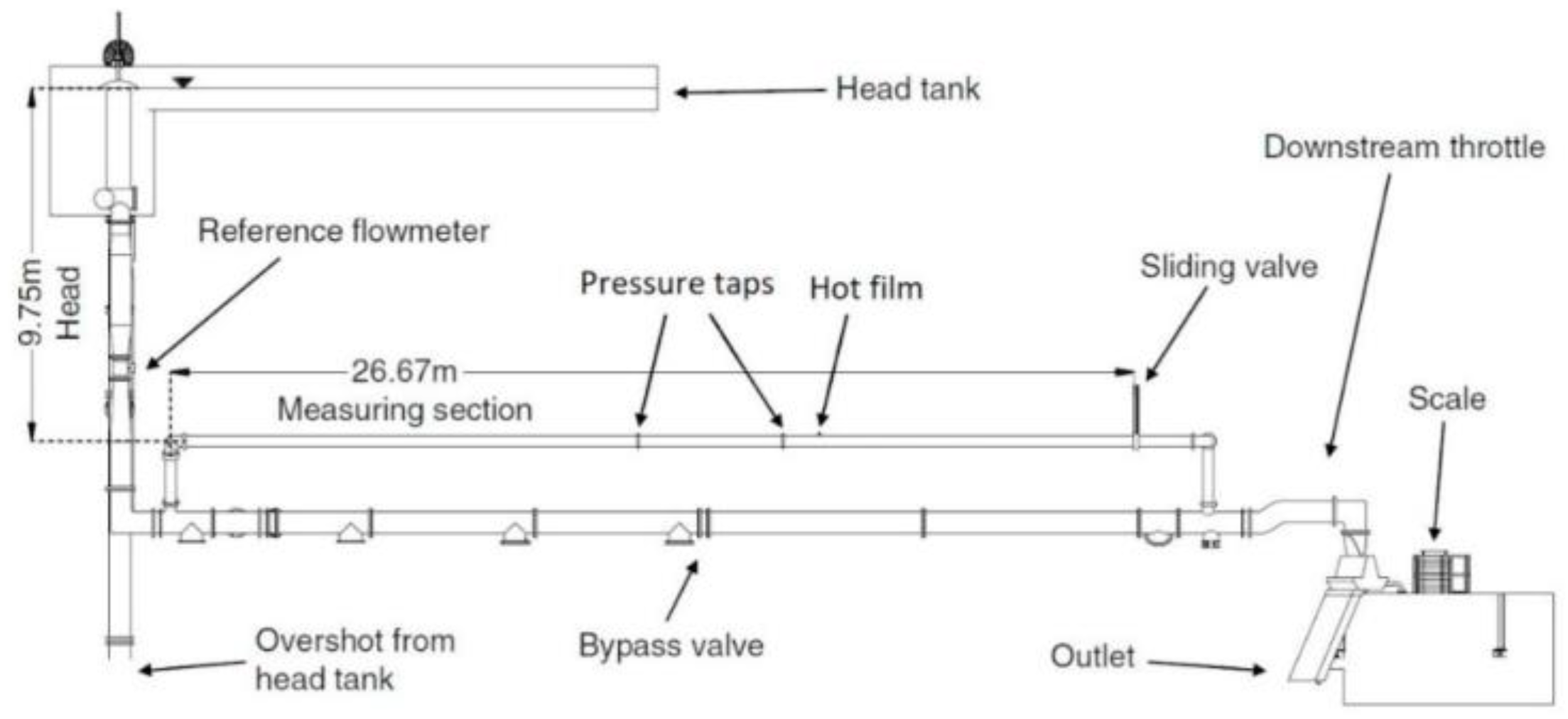
The analyzed test case of this study is based on an experimental investigation conducted by Sundstrom et al. [17]. The geometry is a straight pipe with a constant internal diameter of 300 mm. A schematic of the test apparatus used for the experiment is shown in Figure 1. The water flows by gravity from a head tank, situated H = 9.75 m above the measuring section. The maximum flow rate is Q = 0.410 m3/s.
A gate valve is used to decrease the flow rate which can be reduced to zero in 4.68 s. A differential pressure transducer with a range of 0–5 bar and an accuracy of 0.04% of full scale measures the pressure variation between two sections, 11 and 15 m upstream of the valve. In addition, the wall shear stress at the cross-section 10 m upstream of the valve was measured using a hot-film probe. The flow rate during the measurement was Q = 0.169 m3/s, i.e., a Reynolds number Re = 7 × 10⁵.
The geometry is considered a straight pipe, and other parts such as elbows and fittings are eliminated in the CFD geometry for simplification. The length of the pipe is considered to be 36 m to match the water hammer period obtained in the experiments.
2.2. Mathematical Modelling
The continuity and momentum equations for a time-dependent isothermal compressible turbulent flow are given by:
where P, ρ, Ui, and µ are the pressure, fluid density, mean velocity, and fluid dynamic viscosity, respectively. To model the Reynolds shear stress term () in the turbulent flow, the low Reynolds k-ω SST model [18] is used. Ref. [12] demonstrated that low-Re SST k-ω turbulence models predict more acceptable results for pressure variation during water hammer than high-Re turbulence models. The k-ε model with wall functions cannot capture the variation of the velocity profile close to the wall. This turbulence model was used in similar studies with satisfactory results [4,10,11,12]. To model the fluid compressibility, Hooke’s law with Equation (4) describing the variation of the density with the pressure [19] is used. The effects of pipe elasticity [11] are accounted in modified bulk modulus , Equation (5), where E, e, and D are the Young’s modulus of elasticity, thickness, and pipe diameter, respectively.
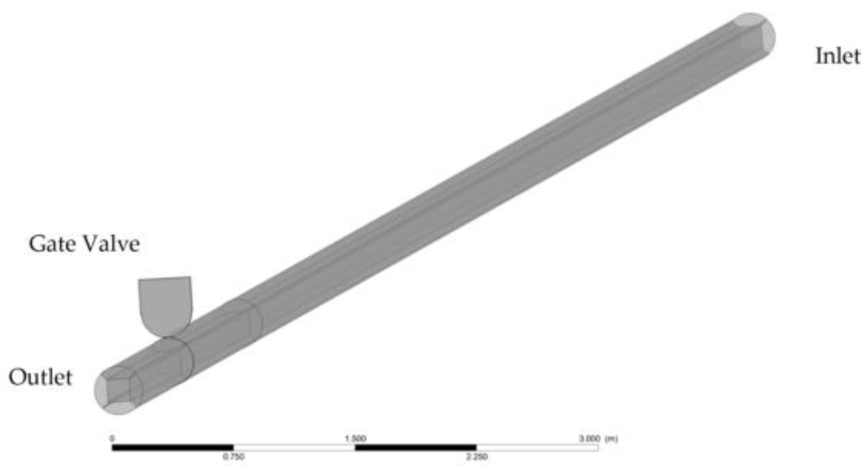
To eliminate the impact of the outlet boundary condition, the pipe was extended for 6 m downstream the valve, i.e., 20 × D. The total pressure value at the inlet ([) is adjusted in the steady-state simulation to match the experiment’s flow rate, while at the outlet the atmospheric pressure () is used. The boundary condition and the geometry used for the simulation is shown in Figure 2. A converged steady-state solution with a constant flow rate is employed for the initial condition of the transient simulation including the valve movement. A root-mean-square (RMS) residual level of 10-5 is considered for the convergence of the variables.
2.3. Valve Closure Modeling
Three methods were used to model the valve closure: dynamic mesh, mesh motion, and immersed solid. Two codes were used: Ansys-Fluent and Ansys-CFX as immersed solid is unavailable in Ansys-Fluent and the sliding mesh is not available for domain translation in Ansys-CFX.
2.3.1. Immersed Solid Method
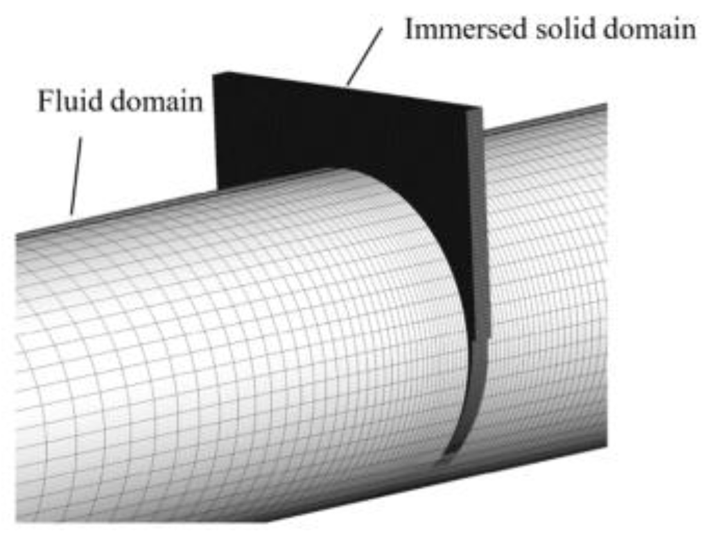
In the immersed solid method, the valve body is modelled by the domain named immersed solid domain. The immersed solid domain overlaps the fluid domain, represented by a pipe, as the valve enters the pipe, shown in Figure 3. In this method, there is no mesh deformation, re-meshing, or domain interface, making this method simple to implement and computationally effective. Instead, the region of overlap between the fluid domain and immersed solid domain is identified at each time step of the simulation. At the fluid cells overlapping with the immersed solid cells, a source term is defined in the momentum equation to match the fluid velocity to the solid velocity [20]. As the momentum equations enforce the fluid velocity in the fluid region to be the same as the velocity of the immersed solid, it will not precisely model the same physical phenomena. The part of the fluid domain that overlaps with the immersed solid has a downward velocity similar to the gate. However, there should be no water there. Moreover, the estimation of the source term by the solver could lead to some leakage through the immersed solid [16].
2.3.2. Dynamic Mesh
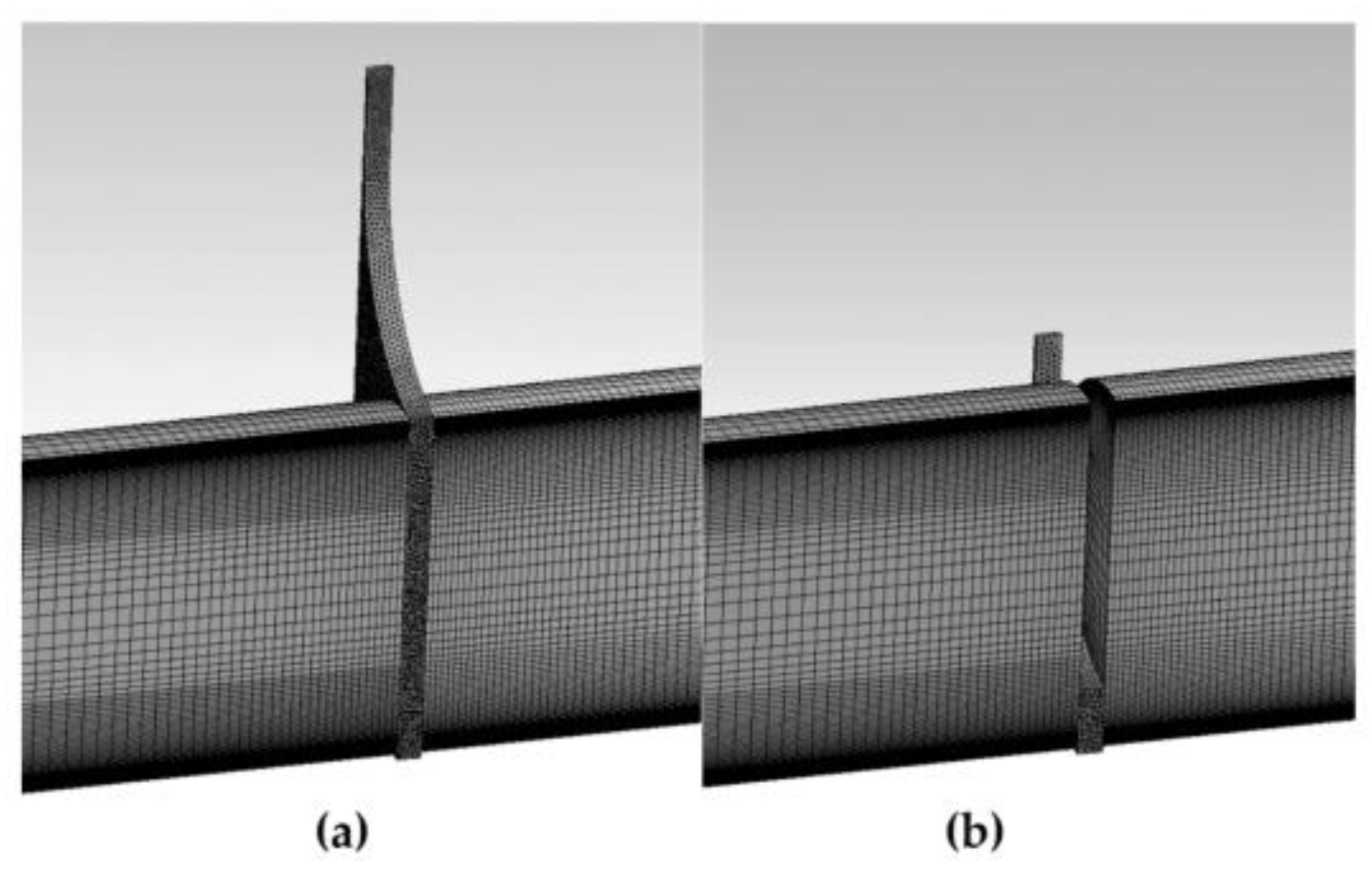
In the dynamic mesh method, the complete geometry is modelled with 3 domains: the pipe upstream the valve (domain 1), the space to be occupied by the valve in the pipe (domain 2), and the pipe downstream the valve (domain 3), see Figure 4. The lower part of the valve is represented by the upper part of domain 2. As the valve moves inside the pipe, the upper part of domain 2 moves downward, decreasing the volume of domain 2. The movement shall be normal to the boundary and involves mesh deformation and remeshing. As the valve moves inside the pipe, a space modelling the valve, i.e., a solid, appears between domain 1 and domain 3. Interfaces connect the domains which are updated at each time step.
The dynamic mesh is available in Ansys-Fluent allowing smoothing and re-meshing at each time step. Re-meshing is not available at Ansys-CFX; therefore, Ansys-Fluent is used. Both smoothing and re-meshing are used in mesh deformation. The spring/Laplacian-based smoothing method [21] is employed. According to Hooke’s law, a displacement at a moving boundary node will produce a force proportional to the displacement along the grid. The spring/Laplacian smoothing process moves each mesh vertex closer to its surrounding vertex’s geometric center. Cell deformation with smoothing for considerable displacement becomes excessively skewed [21]. Therefore, re-meshing is used when the quality of the mesh decreases below thresholds; the maximum face skewness (0.5) and maximum cell skewness (0.7). Moreover, only triangular or tetrahedral mesh can be used for re-meshing in the dynamic mesh zone.
The re-meshing makes the simulation more time-consuming and expensive compared to the other two methods. At the end of the valve closure, as the space to re-mesh is smaller and smaller, there is a higher possibility of divergence as it is challenging to ensure a good quality. To solve the problem, a lower under-relaxation factor value and a higher number of iterations at each time step is considered, making the simulation even more expensive. Moreover, as the mesh is updated at each time step through deformation or a new mesh, the data from the previous time step will be interpolated, which could cause some errors.
2.3.3. Sliding Mesh
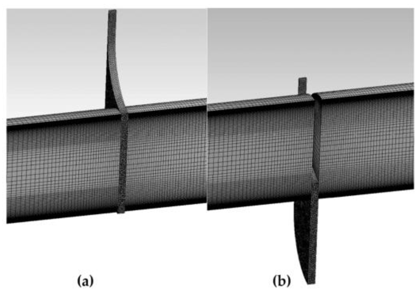
In the sliding mesh method, the computational domain is represented by three sub-domains, like for the dynamic mesh. However, domain 2 is now sliding; thus, no deformation or mesh adjustment is performed. The other fluid zones are stationary. The mesh representing the volume to be occupied by the gate, domain 2, moves along the interface relative to the stationary mesh. After sliding the domain, the interface re-establishes the zone connectivity at each time step. Each zone (stationary or sliding) has at least one “interface zone” around it where it intersects with the neighboring cell zone. In the case of non-overlapping boundaries, wall boundaries are considered. Since the mesh does not deform, the downward movement of the valve zone extends at the bottom of the pipe, shown in Figure 5. Therefore, the bottom of the pipe at the position of domain 2 presents a cavity during the transient that does not present in reality. This could be why dynamic mesh is used for all previous research on gate valve closure [4,10,11]. However, as the valve body thickness is small compared to the pipe’s diameter (0.06 × D), it may have a neglectable effect on the results compared to the expensive method such as the dynamic mesh method. The axial and rotational sliding of mesh are available in Ansys-Fluent; however, the axial movement is not available at Ansys-CFX.
2.4. Computational Setup
As mentioned, all methods are not available in both ANSYS-CFX and ANSYS-Fluent. Therefore, both solvers are employed based on the valve closure method. For the immersed solid method, ANSYS-CFX is used to solve the continuity, momentum, turbulence eddy frequency, and turbulence kinetic energy equations using the coupled finite volume method. The high-resolution scheme is used to solve the terms in the mentioned equations. The high-resolution scheme in CFX is equilibrium to upwind with the number of iterations to increase accuracy. Moreover, CFX uses a couple solver.
The pipe mesh is made of hexahedral elements with a finer mesh in the viscous sublayer to obtain y+ < 1 at the wall. Moreover, a finer mesh close to the valve is also used to have better accuracy, see Figure 6.
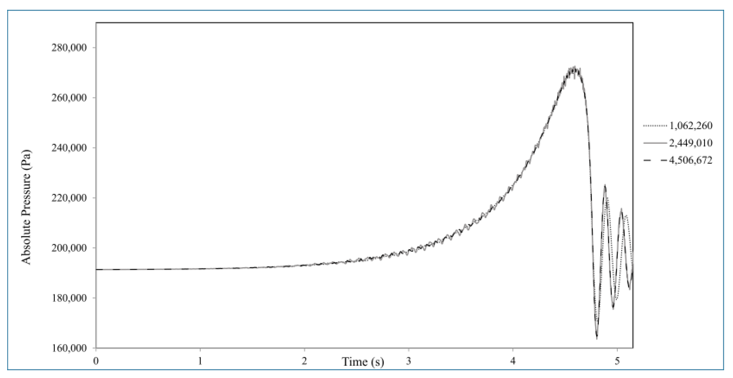
Three different meshes, including both fluid and immersed solid, with grid nodes of 1 × 10⁶, 2.4 × 10⁶, and 4.5 × 10⁶ are made using a time step size of 0.1 ms to study the effect of the mesh on the transient simulation solution. The average aspect ratio is around 1021, and the skewness is 0.13.
The average absolute pressure variation at the surface 11 m upstream of the valve is monitored for the three grids during the valve closure and is presented in Figure 7. This point is one of the points that were later used for validation in the differential pressure measurement. The coarse grids predict different results, frequency, and amplitude of the pressure oscillations. The denser and medium grids present similar results. Therefore, the mesh with 2.4 × 10⁶ nodes is considered for the simulation.
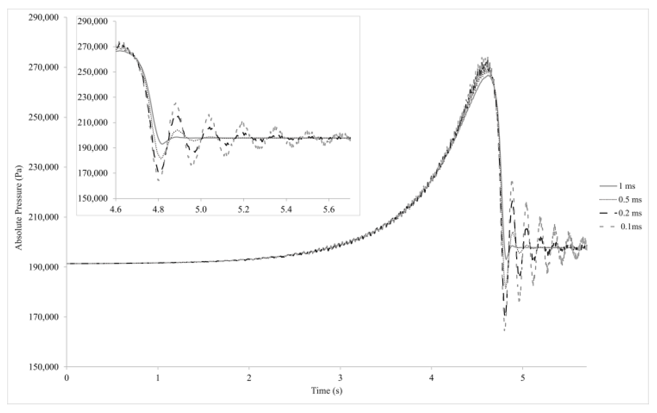
Four time steps ranging from 1 ms to 0.1 ms were applied to the simulation to study the result’s sensitivity to the time step size. The larger time step is not able to predict the pressure oscillations (Figure 8). By reducing the time step size, the oscillation’s amplitude increases and becomes less sensitive to it. A time step size 0.1 ms is considered for independent simulation, which is used in a similar simulation by Kalantar et al. [16]. With a smaller time step, the simulation became too long and gave unphysical results.
For modelling the valve movement with the dynamic mesh method, ANSYS-Fluent is employed. SIMPLE algorithm is used for solving the coupled equations of motion using the finite volume method. The third-order monotonic upwind method (MUSCL) is employed to discretize all transport equations’ non-linear convective terms. A similar number of the elements (2.2 mil grid nodes) and time step (0.1 ms) to Refs. [4,10] are employed for the simulations. In the dynamic mesh method, the maximum face skewness of 0.5 and the maximum cell skewness of 0.7 are considered as the threshold for re-meshing.
For the sliding mesh, ANSYS-Fluent with a similar configuration is used. However, the domain slides and does not need any smoothing or re-meshing.
3. Results
3.1. Pressure Variation
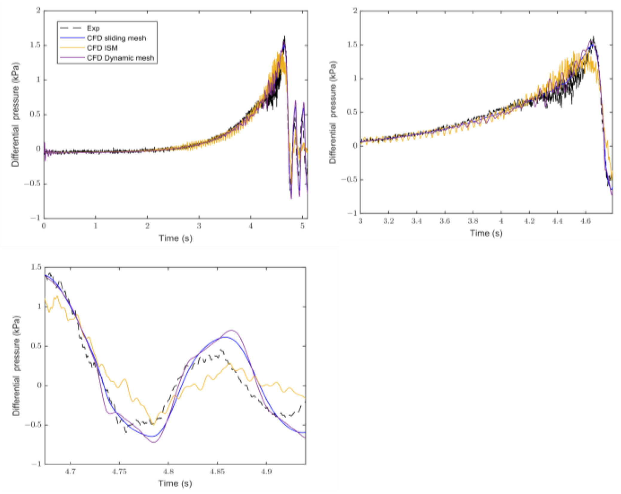
The result of the simulations with different valve modelling has been validated with experimental data from Ref. [17]. The differential pressure variation at the pressure tap between two cross-sections, 11 m and 15 m upstream of the valve, is compared with experimental data in Figure 9. The numerical pressure is obtained at the position of the experimental pressure taps. The maximum peak is lower than the experimental one for the immersed solid method. After the supposed complete valve closure, there is a leakage flow rate, 0.06% of the initial flow rate. This leakage also happens during the valve movement, which leads to a delay in the flow deceleration and thus conversion of momentum into pressure which can be seen in the small delay of pressure the rise before t = 4 s in Figure 9. The underestimation of the maximum peak is certainly related to the leakage and delay in the flow reduction, which affects the maximum pressure rise. The pressure oscillations after the valve closure are also underestimated, which could be for the same reason. Moreover, possible source term estimation errors may add a fluctuation to the main phenomenon, as seen in Figure 9.
The maximum pressure peak in the immersed solid method happens earlier than the experimental one and other CFD results, about 0.1 s. It could be the effect of the downward movement of the water in the fluid zone overlapping the immersed solid. As mentioned, part of the fluid domain overlapping the immersed solid has a downward velocity similar to the gate. However, there should be no water there.
Fluctuations are observed at the start of the valve movement for the dynamic mesh. Changing the mesh at each time step, extrapolation of data to new mesh and skewed mesh during the smoothing leads to error in the simulation, which may be the reason for the instability. Smoothing and re-meshing lead to a higher deviation from the experiment compared to results from sliding mesh, with high-quality mesh.
The sliding mesh technic has a better agreement in predicting the maximum pressure peak and oscillation after the valve closure than the immersed solid and dynamic mesh methods. This method models the same phenomena that happen compared to the immersed solid method. Furthermore, the sliding mesh method uses a higher-quality grid and predicts pressure variation with less fluctuation than the dynamic mesh. Moreover, this method is less computationally intensive than the dynamic mesh.
Results from the sliding and dynamic mesh methods overestimate the pressure oscillations after the valve closure compared to the experimental ones. The reason could be the geometrical differences, simplification in the geometry, and the experimental results’ sensitivity to the tubing in differential pressure measurement. The irregularities and the tank in the test rig may have a higher damping ratio compared to the geometry used in the simulation.
For a better comparison, the predicted differential pressure during the valve movement closure with the sliding mesh method, the closest model to the experiment minus the experimental value, is presented in Figure 10.
As it can be seen, the highest deviation to the experiment happens at the end of the valve closure, and the simulation underestimates the peak. At this time, the variation of the pressure during the water hammer is maximum and based on Equation (4), the highest fluid density variation occurs.
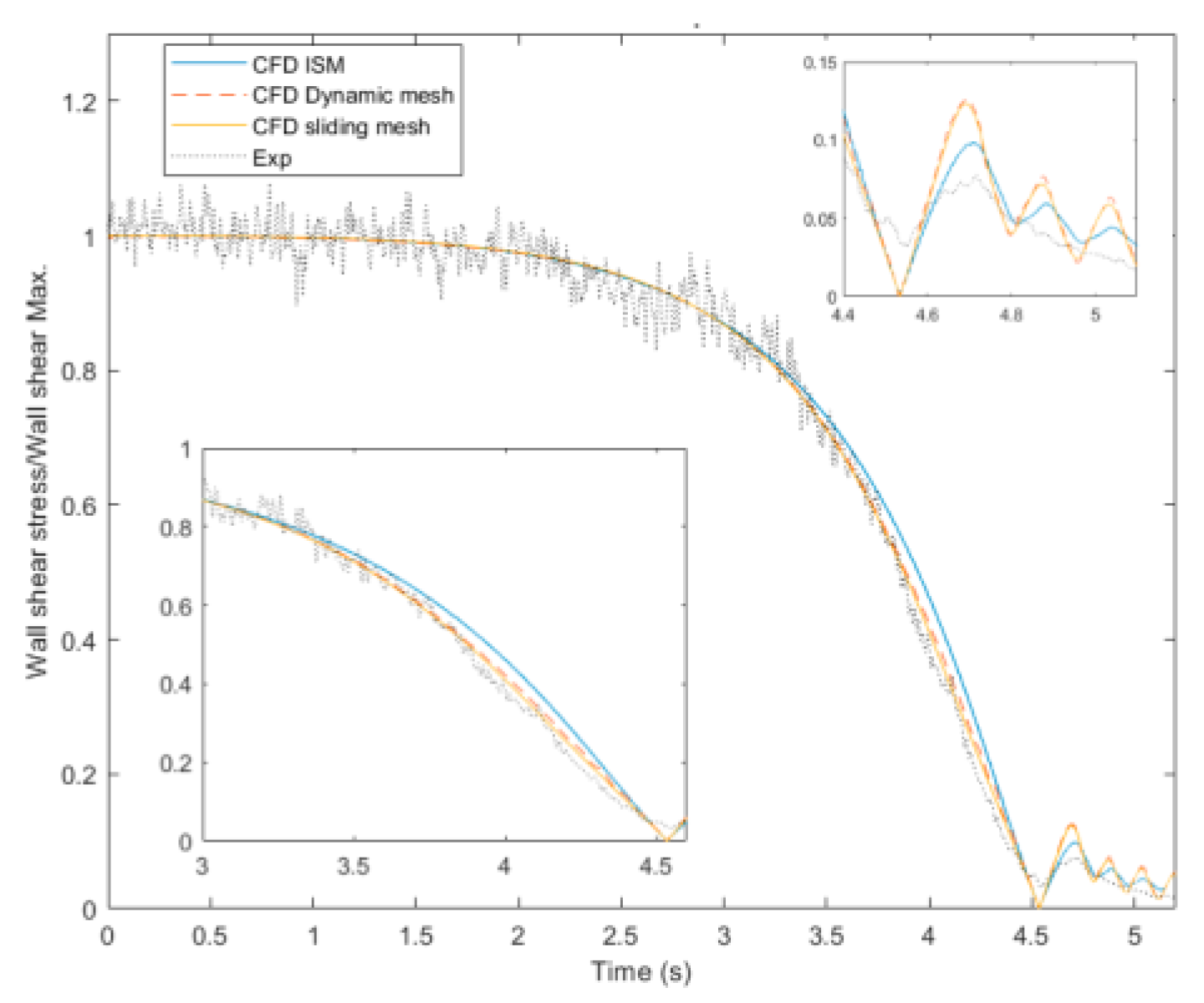
3.2. Wall Shear Stress Variation
The normalized magnitude of the wall shear stress is presented for the different methods used in Figure 11. The results from the sliding mesh agree better than the other methods with the experimental values. The immersed solid method overestimates the wall shear stress between 3 and 4.6 s. The reason could be the delay in flow rate reduction and possible leakage with the method. The dynamic mesh has a good agreement for predicting the wall shear stress during the valve closure. However, there is a slight overestimation of the wall shear stress from 3 to 4.6 s. The sliding mesh has the best agreement for predicting the wall shear stress during the valve closure compared to the other methods. All the methods overestimate the wall shear stress after the valve closure during the oscillations. The irregularities, such as elbow and contractions, and the tanks in the test rig may have a higher damping ratio compared to the simplified geometry used, a single pipe. Therefore, a lower flow rate will be expected during the oscillation compared to the geometry used in the simulation.
3.3. 3D Effects
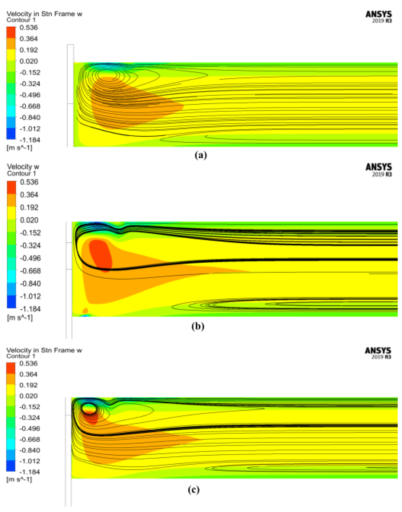
As mentioned, a non-symmetrical recirculation region appears near the gate valve with its movement. Therefore, the flow is 3D close to the valve; however, far from the valve, the flow is 2D. The 3D flow related to the valve closure during the water hammer is visualized by contours of the axial velocity close to the valve at the end of the closure. Streamlines and axial velocity contour of the flow inside the pipe are presented in Figure 12. This non-symmetrical recirculation region extends approximately two to three pipe diameters depending on the simulation method. In Figure 12, the streamlines are presented at time t = 4.75 s; however, the immersed solid method models may have a small time shift regarding the delay in the flow rate reduction. Immersed solid method predicts a shorter length of 3D effect because of possible leakage and weaker water hammer. Dynamic mesh indicates a negative axial velocity at the bottom of the pipe close to the valve, which other methods do not predict. The reason could be the skewed mesh at the end of valve closure, inducing an unphysical value for the velocity profile. The sliding mesh, the most physical method, predicts the most extended 3D effects.
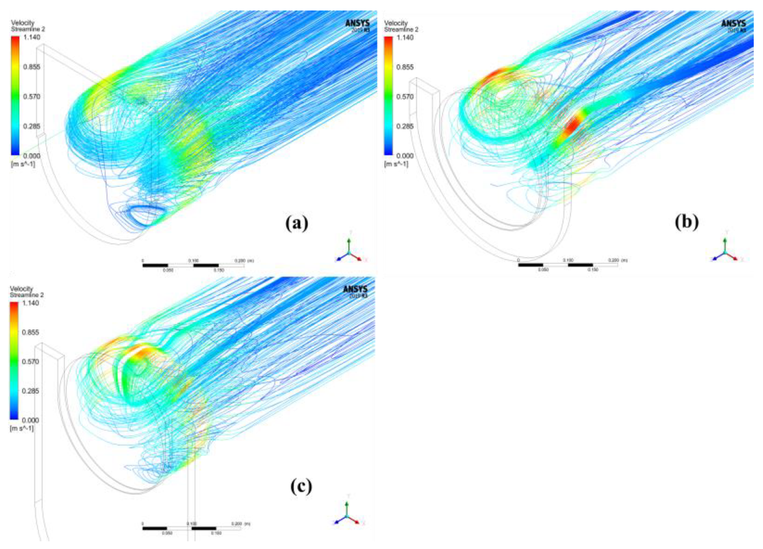
The 3D effect can be observed more accurately with 3D flow streamlines close to the valve at the end of valve closure, shown in Figure 13. The leakage flow can be observed in the 3D streamlines obtained from the immersed solid method. The two-dimensional streamlines cannot show the recirculation zone along to the pipe wall. For the simulations performed using the sliding mesh and dynamic mesh techniques, the recirculation around the top and sides of the pipe wall is similar and recirculation zone at the bottom of the pipe is weaker. However, the recirculation zones close to the top of the pipe are weaker for simulation by the immersed solid technique than other results. It could be related to leakage through the immersed solid during the valve closure. The 3D streamlines predicted a similar 3D structure after the valve closure for simulation using the sliding mesh and dynamic mesh techniques.
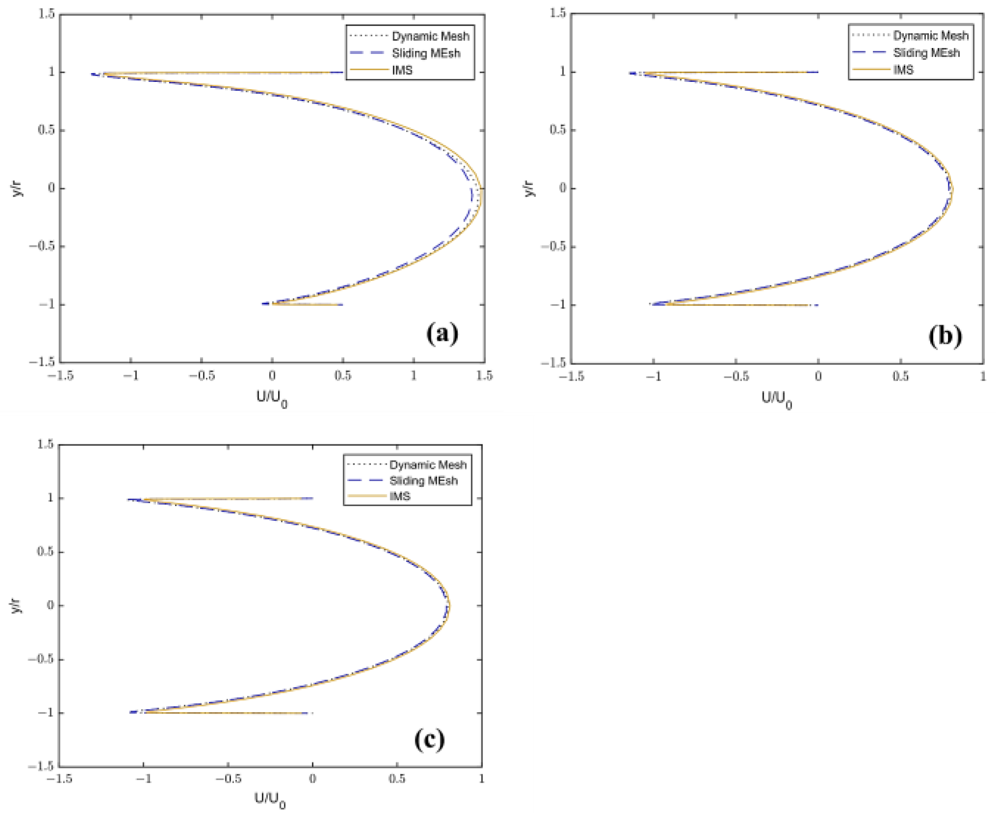
The axial velocity profile at the vertical line with distances 25 cm, 50 cm, and 75 cm upstream of the valve at the end of the valve closure is presented in Figure 14. The velocity profiles are more asymmetrical closer to the valve. The flow field gradually becomes symmetrical away from the valve. By moving from the valve towards the inlet, the 3D effect decreases, and in line ‘’c’’ (with a distance of 75 cm upstream of the valve), the 3D effect ends. Therefore, the pressure measurement for application, like the pressure-time method, shall be performed at a section before this area.
The 3D effect is more significant for the results from sliding mesh and the immersed solid method predicts the least 3D effects because of possible leakage and weaker water hammer.
3.4. Computational Cost
Another essential aspect to consider is the computational cost of each method. Immersed solid method and sliding mesh have quite the same computational cost. For dynamic mesh, the process of re-meshing is added to the calculation. Moreover, the lower quality of regenerated mesh makes it more possible to diverge. Therefore, a lower under-relaxation factor and, consequently, a higher number of iterations per time step is applied in the simulation. The mentioned drawbacks made the computational cost of the dynamic mesh method around three times more than the sliding mesh and immersed solid method. The details of the computational resources and time used for the simulation with the different methods are summarized in Table 1.
4. Conclusions and Discussion
The current method presents a CFD simulation of the water hammer caused by the axial movement of a gate valve in a straight pipe. Three techniques for modelling valve closure are employed, including immersed solid (Ansys-CFX), dynamic, and sliding mesh methods (Ansys-Fluent). The results show that immersed solid method has a delay in flow rate reduction, which underestimates differential pressure rise and overestimates wall shear stress close to the end of valve closure. The dynamic mesh method models the same physical phenomenon. However, it is more time-consuming and three times more expensive in terms of computational cost than other methods. Furthermore, the dynamic mesh was unstable, with the possibility of divergence.
As an inexpensive and stable technique, the sliding mesh method predicts the closest result to the experimental value. It was proved that for a thin gate valve, the axial movement of the valve can be modelled by mesh movement without any mesh deformation. This method can predict more physical results for the conditions mentioned in the paper.
Author Contributions
Conceptualization, M.K.N. and M.J.C.; methodology, M.K.N. and M.J.C.; software, M.K.N.; validation, M.K.N.; formal analysis, M.K.N.; investigation, M.K.N., G.D. and M.J.C.; resources, M.J.C.; data curation, M.K.N.; writing—original draft preparation, M.K.N.; writing—review and editing, P.J., G.D. and M.J.C.; visualization, M.K.N.; supervision, P.J., G.D. and M.J.C.; project administration, M.J.C.; funding acquisition, M.J.C. All authors have read and agreed to the published version of the manuscript.
Funding
This research was funded by “Swedish Hydropower Centre-SVC” and “Luleå University of Technology-LTU”. “Swedish Hydropower Centre-SVC” established by the Swedish Energy Agency, Elforsk and Svenska Kraftnät, together with the Luleå University of Technology, The Royal Institute of Technology, Chalmers University of Technology, and Uppsala University.
Data Availability Statement
Data available on request due to restrictions privacy.
Acknowledgments
The research presented was carried out as a part of “Swedish Hydropower Centre-SVC” established by the Swedish Energy Agency, Elforsk and Svenska Kraftnät, together with the Luleå University of Technology, The Royal Institute of Technology, Chalmers University of Technology, and Uppsala University.
Conflicts of Interest
The authors declare no conflict of interest.
References
- IEC 60041, I.; Field Acceptance Tests to Determine the Hydraulic Performance of Hydraulic Turbines, Storage Pumps and Pump-Turbines. International Electrotechnical Commission: Geneva, Switzerland, 1991.
- Zhang, X.; Cheng, Y.; Xia, L.; Yang, J. CFD Simulation of Reverse Water-Hammer Induced by Collapse of Draft-Tube Cavity in a Model Pump-Turbine during Runaway Process. In Proceedings of the IOP Conference Series: Earth and Environmental Science, Grenoble, France, 4–8 July 2016; Volume 49. [Google Scholar]
- Wu, D.; Yang, S.; Wu, P.; Wang, L. MOC-CFD Coupled Approach for the Analysis of the Fluid Dynamic Interaction between Water Hammer and Pump. J. Hydraul. Eng. 2015, 141, 06015003. [Google Scholar] [CrossRef]
- Saemi, S.; Raisee, M.; Cervantes, M.J.; Nourbakhsh, A. Numerical Investigation of the Pressure-Time Method Considering Pipe with Variable Cross Section. J. Fluids Eng. Trans. ASME 2018, 140, 101401. [Google Scholar] [CrossRef]
- Saemi, S.D.; Raisee, M.; Cervantes, M.J.; Nourbakhsh, A. Computation of Laminar and Turbulent Water Hammer Flows. In Proceedings of the 11th World Congress on Computational Mechanics (WCCM XI) 5th European Conference on Computational Mechanics (ECCM V) 6th European Conference on Computational Fluid Dynamics (ECFD VI), Barcelona, Spain, 20–25 June 2014. [Google Scholar]
- Martin, N.M.C.; Wahba, E.M. On the Hierarchy of Models for Pipe Transients: From Quasi-Two-Dimensional Water Hammer Models to Full Three-Dimensional Computational Fluid Dynamics Models. J. Press. Vessel. Technol. Trans. ASME 2022, 144, 021402. [Google Scholar] [CrossRef]
- Nikpour, M.R.; Nazemi, A.H.; Dalir, A.H.; Shoja, F.; Varjavand, P. Experimental and Numerical Simulation of Water Hammer. Arab. J. Sci. Eng. 2014, 39, 2669–2675. [Google Scholar] [CrossRef]
- Li, J.; Wu, P.; Yang, J. Cfd Numerical Simulation of Water Hammer in Pipeline Based on the Navier-Stokes Equation. In Proceedings of theV European Conference on Computational Fluid Dynamics, Lisbon, Portugal, 14–17 June 2010. [Google Scholar]
- Mandair, S.; Magnan, R.; Morissette, J.-F.; Karney, B. Energy-Based Evaluation of 1D Unsteady Friction Models for Classic Laminar Water Hammer with Comparison to CFD. J. Hydraul. Eng. 2020, 146, 04019072. [Google Scholar] [CrossRef]
- Saemi, S.; Cervantes, M.J.; Raisee, M.; Nourbakhsh, A. Numerical Investigation of the Pressure-Time Method. Flow Meas. Instrum. 2017, 55, 44–58. [Google Scholar] [CrossRef]
- Saemi, S.; Sundström, L.R.J.; Cervantes, M.J.; Raisee, M. Evaluation of Transient Effects in the Pressure-Time Method. Flow Meas. Instrum. 2019, 68, 101581. [Google Scholar] [CrossRef]
- SaemI, S.; Raisee, M.; Cervantes, M.J.; Nourbakhsh, A. Computation of Two- and Three-Dimensional Water Hammer Flows. J. Hydraul. Res. 2019, 57, 386–404. [Google Scholar] [CrossRef]
- Wang, H.; Zhou, L.; Liu, D.; Karney, B.; Wang, P.; Xia, L.; Ma, J.; Xu, C. CFD Approach for Column Separation in Water Pipelines. J. Hydraul. Eng. 2016, 142, 04016036. [Google Scholar] [CrossRef] [Green Version]
- Yang, S.; Wu, D.; Lai, Z.; Du, T. Three-Dimensional Computational Fluid Dynamics Simulation of Valve-Induced Water Hammer. Proc. Inst. Mech. Eng. C J. Mech. Eng. Sci. 2017, 231, 2263–2274. [Google Scholar] [CrossRef]
- Han, Y.; Shi, W.; Xu, H.; Wang, J.; Zhou, L. Effects of Closing Times and Laws on Water Hammer in a Ball Valve Pipeline. Water 2022, 14, 1497. [Google Scholar] [CrossRef]
- Kalantar, M.; Jonsson, P.; Dunca, G.; Cervantes, M.J. Numerical Investigation of the Pressure-Time Method. IOP Conf. Ser. Earth Environ. Sci. 2022, 1079, 012075. [Google Scholar] [CrossRef]
- Sundstrom, L.R.J.; Cervantes, M.J. Transient Wall Shear Stress Measurements and Estimates at High Reynolds Numbers. Flow Meas. Instrum. 2017, 58, 112–119. [Google Scholar] [CrossRef]
- Menter, F.R. Two-Equation Eddy-Viscosity Turbulence Models for Engineering Applications. AIAA J. 1994, 32, 1598–1605. [Google Scholar] [CrossRef] [Green Version]
- Korteweg, D.J. Ueber Die Fortpflanzungsgeschwindigkeit Des Schalles in Elastischen Röhren. Ann. Phys. 1878, 241, 525–542. [Google Scholar] [CrossRef] [Green Version]
- Yoon, Y.; Park, B.H.; Shim, J.; Han, Y.O.; Hong, B.J.; Yun, S.H. Numerical Simulation of Three-Dimensional External Gear Pump Using Immersed Solid Method. Appl. Therm. Eng. 2017, 118, 539–550. [Google Scholar] [CrossRef]
- ANSYS, Inc. ANSYS Fluent User’s Guide, Release 17.2; ANSYS, Inc.: Canonsburg, PA, USA, 2016. [Google Scholar]
Figure 1.
The water hammer test rig schematic. Figure courtesy of Sundstrom et al. [17].
Figure 1.
The water hammer test rig schematic. Figure courtesy of Sundstrom et al. [17].

Figure 2.
The boundary conditions and geometry used for the simulation.

Figure 3.
Overlapping of the fluid zone and immersed solid zone at time t =4 s (close to the end of the valve closure) in the immersed solid method for modelling valve movement.
Figure 3.
Overlapping of the fluid zone and immersed solid zone at time t =4 s (close to the end of the valve closure) in the immersed solid method for modelling valve movement.

Figure 4.
Dynamic mesh method grid cut in half: (a) before valve movement; (b) at t = 4 s close to the end of valve closure.
Figure 4.
Dynamic mesh method grid cut in half: (a) before valve movement; (b) at t = 4 s close to the end of valve closure.

Figure 5.
Sliding mesh method grid cut in half: (a) at t = 0 s before valve movement; (b) at t = 4 s close to the end of valve closure.
Figure 5.
Sliding mesh method grid cut in half: (a) at t = 0 s before valve movement; (b) at t = 4 s close to the end of valve closure.

Figure 6.
Immersed solid method grid: (a) fine grid near the gate; (b) grid at the pipe cross-section.
Figure 6.
Immersed solid method grid: (a) fine grid near the gate; (b) grid at the pipe cross-section.

Figure 7.
Average absolute pressure monitoring at section 11 m upstream of valve for three different grids.
Figure 7.
Average absolute pressure monitoring at section 11 m upstream of valve for three different grids.

Figure 8.
Average absolute pressure monitoring at section 11 m upstream of valve for four different time steps.
Figure 8.
Average absolute pressure monitoring at section 11 m upstream of valve for four different time steps.

Figure 9.
The variation of differential pressure with time during the valve closure between two cross-sections 11 m and 15 m upstream of the valve.
Figure 9.
The variation of differential pressure with time during the valve closure between two cross-sections 11 m and 15 m upstream of the valve.

Figure 10.
The deviation of estimated differential pressure by sliding mesh with the experiment between two cross-sections 11 m and 15 m upstream of the valve.
Figure 10.
The deviation of estimated differential pressure by sliding mesh with the experiment between two cross-sections 11 m and 15 m upstream of the valve.

Figure 11.
The time variation of the magnitude wall shear stress at cross-sections 10 m upstream of the valve.
Figure 11.
The time variation of the magnitude wall shear stress at cross-sections 10 m upstream of the valve.

Figure 12.
Streamlines and axial velocity contour of the flow inside the pipe at the end of the valve closure: (a) immersed solid method; (b) dynamic mesh; (c) sliding mesh.
Figure 12.
Streamlines and axial velocity contour of the flow inside the pipe at the end of the valve closure: (a) immersed solid method; (b) dynamic mesh; (c) sliding mesh.

Figure 13.
Streamlines of the flow inside the pipe at the end of the valve closure for the different valve modelling method: (a) immersed solid; (b) dynamic mesh; (c) sliding mesh.
Figure 13.
Streamlines of the flow inside the pipe at the end of the valve closure for the different valve modelling method: (a) immersed solid; (b) dynamic mesh; (c) sliding mesh.

Figure 14.
Axial velocity profile at the vertical line with distances of: (a) 25cm; (b) 50 cm; (c) 75 cm upstream of the valve at the end of the valve closure.
Figure 14.
Axial velocity profile at the vertical line with distances of: (a) 25cm; (b) 50 cm; (c) 75 cm upstream of the valve at the end of the valve closure.


Table 1.
Computational resources and time allocated to the simulations.
| Method | Number of CPU (2.60 GHz) | App. Time (h) |
|---|---|---|
| Immersed solid method | 48 | 60 |
| Dynamic mesh method | 48 | 170 |
| Sliding mesh method | 48 | 65 |
Disclaimer/Publisher’s Note: The statements, opinions and data contained in all publications are solely those of the individual author(s) and contributor(s) and not of MDPI and/or the editor(s). MDPI and/or the editor(s) disclaim responsibility for any injury to people or property resulting from any ideas, methods, instructions or products referred to in the content. |
© 2023 by the authors. Licensee MDPI, Basel, Switzerland. This article is an open access article distributed under the terms and conditions of the Creative Commons Attribution (CC BY) license (https://creativecommons.org/licenses/by/4.0/).
Share and Cite
MDPI and ACS Style
Neyestanaki, M.K.; Dunca, G.; Jonsson, P.; Cervantes, M.J. A Comparison of Different Methods for Modelling Water Hammer Valve Closure with CFD. Water 2023, 15, 1510. https://doi.org/10.3390/w15081510
AMA Style
Neyestanaki MK, Dunca G, Jonsson P, Cervantes MJ. A Comparison of Different Methods for Modelling Water Hammer Valve Closure with CFD. Water. 2023; 15(8):1510. https://doi.org/10.3390/w15081510
Chicago/Turabian StyleNeyestanaki, Mehrdad Kalantar, Georgiana Dunca, Pontus Jonsson, and Michel J. Cervantes. 2023. "A Comparison of Different Methods for Modelling Water Hammer Valve Closure with CFD" Water 15, no. 8: 1510. https://doi.org/10.3390/w15081510
Note that from the first issue of 2016, this journal uses article numbers instead of page numbers. See further details here.