


Numerical Simulation of Two-Dimensional Dam Failure and Free-Side Deformation Flow Studies

1
School of Electronics and Information Engineering, Guangdong Ocean University, Zhanjiang 524088, China
2
Ocean College, Zhejiang University, Zhoushan 316021, China
3
Ship and Maritime College, Guangdong Ocean University, Zhanjiang 524088, China
4
School of Maritime Transport, Ningbo University, Ningbo 315211, China
*
Author to whom correspondence should be addressed.
Water 2023, 15(8), 1515; https://doi.org/10.3390/w15081515
Submission received: 28 February 2023
/
Revised: 30 March 2023
/
Accepted: 10 April 2023
/
Published: 13 April 2023
(This article belongs to the Special Issue Application of Spatiotemporal Data in Hydrological Hazards of Drought, Flood and Water Pollution Assessment and Monitoring)
Abstract
:A dam breaking is a major flood catastrophe. The shape, depth, and wave Doppler effect of initial water flow are all modified as a result of the interaction of the water body with downstream structures after a dam breach, forming a diffraction and reflection flow field. This study investigates the dam breaking problem of a single liquid, by creating a two-dimensional simplified numerical model using the VOF approach, analysing the interaction and effect between barriers of various forms and the dam failure flow, and explains the problem of a complex flow mechanism involving significant deformation of the free surface of a medium. According to the findings, obstacles of varying forms could obstruct the dam break’s water flow to various degrees, and the viscous dissipation characteristic of the water body at the edge of the obstacle is closely related to the slope of the site. The numerical simulation presented in this study is validated, demonstrating its accuracy for both the gate-pulling and downstream wet-bed scenarios.
1. Introduction
Dam collapse, or dam body failure, is a common flow phenomenon in water conservation systems. A massive volume of water is abruptly released out of control when the dam body breaks, creating a flood that spreads quickly downstream in the shape of a surge wave and inflicting catastrophic destruction to lives and property in the downstream region [1]. There have been many significant dam failure disasters in recent decades that left a terrible toll in terms of both human lives and property destruction [2]. For example, the 1963 failure of Vajont dam in Italy caused 2600 deaths, the 1976 failure of Teton dam in America caused hundred deaths and economic loss about 1 billion dollars, and the 1993 failure of Gouhou dam in China caused 300 deaths. The statistical analysis of 534 dam failures from 43 countries before 1974 indicated that earth-rock dam failures accounted for the largest proportion of all failures and included 49% caused by overtopping, 28% seepage in dam body and 29% seepage in foundation. There were about 3498 dam failures in China between 1954 and 2006, 90% of which were earth dams, especially homogeneous earth dams which account for 85% of all these failures [3,4]. To prevent flooding and limit fatalities, it is crucial to forecast free surfaces, water depths, and wave changes because of dam breakdown.
With the development of computers and numerical methods, numerical simulation has proved to be an effective means to study the evolution of dam failure flow and is widely used [5]. Dam collapse is a typical free-plane large-deformation flow problem, and correctly modelling the process of dam failure depends on perfectly capturing the free surface. For complicated water epidemics after dam collapse, Kocaman [6,7,8,9,10] carried out a number of model experiments and numerical simulations, providing benchmark model for later researchers. Up to now, various numerical models are proposed to study the free surface problem of dam failure simulation, such as the VOF (volume of fluid) method, the SPH (smoothed particle hydrodynamics) method, the finite element method, and artificial intelligence models.
The VOF multiphase model belongs to the family of Interface-capturing methods that predict the distribution and the movement of the interface of immiscible phases [11,12,13]. This modeling approach assumes that the mesh resolution is sufficient to resolve the position and the shape of the interface between the phases. Issakhov [14] simulated the movement of macro particles on the water’s surface in the dam’s water flow using the VOF method in conjunction with a discrete phase model and macro particle model. Mokrani and Abadie [15] addressed the problem of numerical simulation of the dynamic loads generated during a dry dam break flow impact on a wall using the VOF model. The conclusion could be drawn that the pressure field in the vicinity of the wall right after impact was highly variable in space and time. Khoshkonesh et al. [16] evaluated the effects of the opening width of a dam site on the evolution of partial dam break waves over a fixed dry bed. The VOF method was also used to scrutinize the propagation of the dam break free surface. The results showed that the VOF model could accurately predict the three-dimensional features of the partial dam break wave. However, the model performance was highly dependent on the overall mesh resolution and model parameters. Munoz and Constantinescu [17] presented 3-D dam break flow simulations using the VOF approach. It was found that dam break flow may be subject to strong 3-D effects. The VOF method determines the interface position by tracking the volume fraction of a phase of fluid in the grid, which has the advantages of less mass loss, less computational complexity, high accuracy, and is widely used.
The SPH method Is totally mesh free and It has been proven to be effective In tracking large free surface deformations [18,19,20]. The basic idea of the SPH method is to describe a continuous fluid (or solid) as an interacting group of particles. Each material point carries various physical quantities, such as mass and velocity. By solving the dynamic equations of a group of particles and tracking the trajectory of each particle, the mechanical behavior of the entire system is obtained. Soleimani [21] utilized the SPH method to model the induced material flow of a double liquid dam breakdown in the presence of various obstructions. Gu et al. [22] simulated the flow mechanism of a three-dimensional dam breakdown using the Level-Set approach. A dam collapse flood wave computation model based on CE/SE format was created by Zhang et al. [23]. Miao et al. [24] used the SPH method to simulate the flow issue of a two-dimensional dam failure on the exterior and performed an initial analysis of flow and energy dissipation of various downstream barriers. Xu et al. [25] simulated three-dimensional dam break flows against various forms of the obstacle using the SPH method. The results showed that the SPH method could handle 3D large deformation flows with any complex boundaries accurately. According to the literature, the VOF method (based on the Euler model) and the SPH method (based on Lagrange model) are the two most often utilized models in the numerical modelling of the free surface of dam breaks.
The finite element method is a numerical method used to obtain the solution of differential equations [26,27,28]. Completion using this method produces an approximation solution in the form of a function on each element such that these functions are continuous with each other [29]. This method can also be used to calculate the free surface of dam breaks. For example, Savant et al. [30] presented an implicit finite element hydrodynamic model for dam and levee breach. The unstructured, implicit, Petrov-Galerkin finite element model relied on computed residuals to automatically adjust the time-step size. Zhang et al. [31] evaluated a three-dimensional unstructured-mesh finite element model for dam break floods through three test cases. Other methods, such as a fast data driven method based on the artificial intelligence (AI), can also help to analyze the flow problems of two-dimensional dam breaks [32,33].
A dam breakdown would generate massive flood waves, transport sediment, induce landform erosion, and result in minor adjustments. Since an unstable and rapidly changing complex flow will also result in significant devastation and fatalities [34,35,36,37,38,39,40,41]. The appearance of the downstream channel may have a significant impact on the water flow structure, maximum depth, and speed of wave propagation during dam breaking wave propagation. When there are wharfs, bridge piers, and other structures in the river, the dam break water flow will also be hampered. A diffraction and reflection flow field will develop around the structures, which will negatively influence the flood’s discharge as well as the structures themselves. Dam water flow will have a significant influence on structures, putting them to the test in terms of strength and stability [42,43,44,45,46].
Much research on dam break flow under various obstacles has been conducted to date, but the study of the interaction mechanism between water flow and barriers, as well as the effect of obstacles on dam break waves, is still insufficient. To investigate the influence of different-shaped obstacles on the dam break flow and evaluate the action mechanism of the complex flow problem of large deformation of the free liquid surface. This paper incorporates the single-liquid dam break problem and uses the VOF method to construct a corresponding two-dimensional simplified numerical model for this case. The simulation results of the dam collapse under the conditions of the gate being pulled out and the downstream with a wet bed are also shown in this research. The rest of the paper is organized as follows: Section 2 presents the numerical models including governing equations and the VOF method. Section 3 and Section 4 simulate the single liquid dam failure with different shapes of obstacles and wet bed downstream, respectively. The free surface, the maximum height of the water column on the left wall and the pressure of obstacles with different shapes are studied. Section 5 compares and analyzes the free surface flow field distribution of dam failure with and without gate. Finally, the conclusions drawn from this study are depicted in Section 6.
2. Numerical Models and the Proposed Method
2.1. Governing Equations
The fundamental laws that govern the mechanics of fluids and solids are the conservation of mass, linear momentum, angular momentum, and energy [47,48]. In this paper, they can be summarized by a two-dimensional continuity equation and Navier-Stokes equations in vector form:
where μeff = μ + μt, μ is the dynamic viscosity, μt is the turbulence viscosity, v is the flow velocity, t is the time, p is the pressure, ρ is the density, fb is the mean external strength of the body.
In CFD simulation, Reynolds-Averaged Navier-Stokes (RANS) turbulence models provide closure relations for the RANS, that govern the transport of the mean flow quantities. To obtain the Reynolds-Averaged Navier-Stokes equations, each solution variable ϕ in the instantaneous Navier-Stokes equations is decomposed into its mean, or averaged, value and its fluctuating component ϕ’:
where ϕ represents velocity components, pressure, energy, or species concentration.
The averaging process may be thought of as time-averaging for steady-state situations and ensemble averaging for repeatable transient situations. Inserting the decomposed solution variables into the Navier-Stokes equations results in equations for the mean quantities.
The mean mass and momentum transport equations can be written as:
where, ρ is the density. is the mean velocity. is the mean pressure. I is the identity tensor. is the mean viscous stress tensor. fb is the resultant of the body force (such as gravity or centrifugal forces).
These equations are essentially identical to the original Navier-Stokes equations, except that an additional term now appears in the momentum and energy transport equations. This additional term is the so-called the stress tensor.
2.2. VOF Method
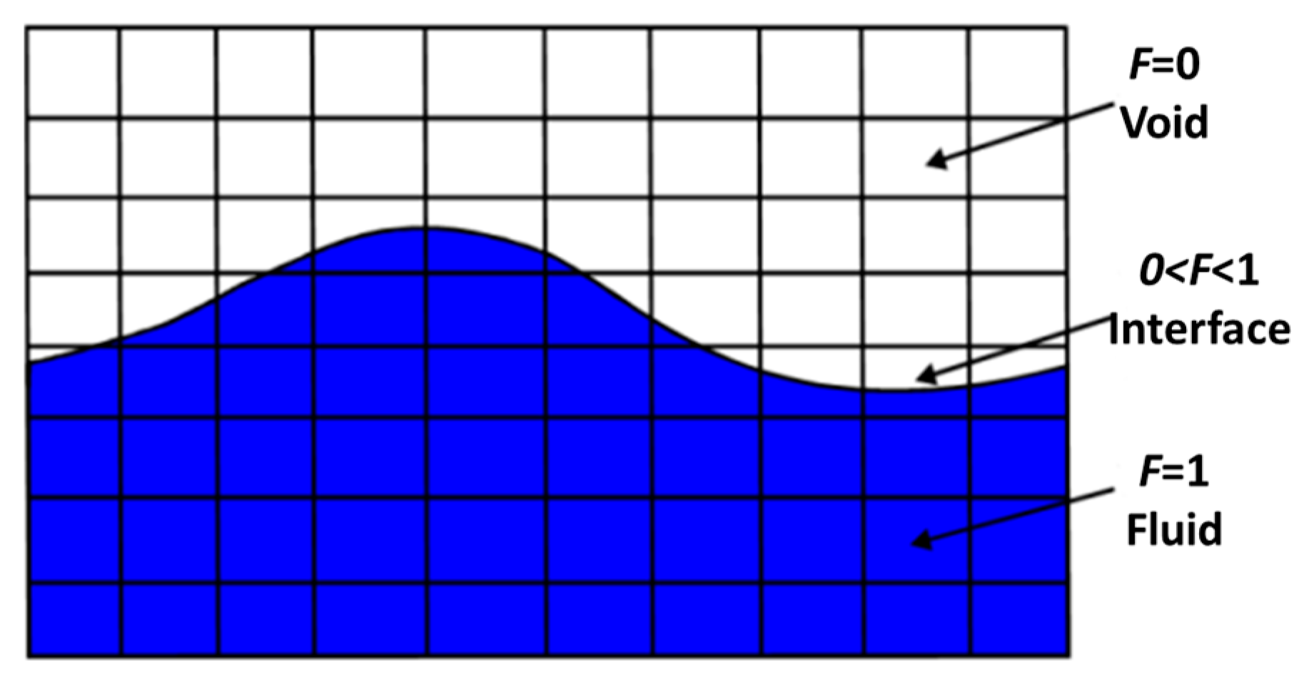
The volume of fluid (VOF) method is used to capture the evolution of free surface for the two-phase flow. The Volume of Fluid (VOF) multiphase model belongs to the family of interface-capturing methods that predict the distribution and the movement of the interface of immiscible phases. This modeling approach assumes that the mesh resolution is sufficient to resolve the position and the shape of the interface between the phases.
The distribution of phases and the position of the interface are described by the fields of phase volume fraction Fi. The volume fraction of phase i is defined as:
where Vi is the volume of phase i in the cell and V is the volume of the cell. The volume fractions of all phases in a cell must sum up to one:
where N is the total number of phases.
Depending on the value of the volume fraction, the presence of different phases or fluids in a cell can be distinguished:
Fi = 0 means that the cell is completely void of phase i;
Fi = 1 means that the cell is completely filled with phase i;
0 < Fi < 1 means that values between the two limits indicate the presence of an interface between phases. The VOF model is shown in Figure 1.
The material properties that are calculated in the cells containing the interface depend on the material properties of the constituent fluids. The fluids that are present in the same interface-containing cell are treated as a mixture:
where ρi is the density, μi is the dynamic viscosity, and (Cp)i is the specific heat of phase i.
The distribution of phase i is driven by the phase mass conservation equation:
where a is the surface area vector, v is the mixture (mass-averaged) velocity, vd,i is the diffusion velocity, Sαi is a user-defined source term of phase i, and Dρi/Dt is the material or Lagrangian derivative of the phase densities ρi.
3. Single Liquid Dam Failure Simulation with Different Shapes of Obstacles Downstream
3.1. Basic Calculation Model Parameters
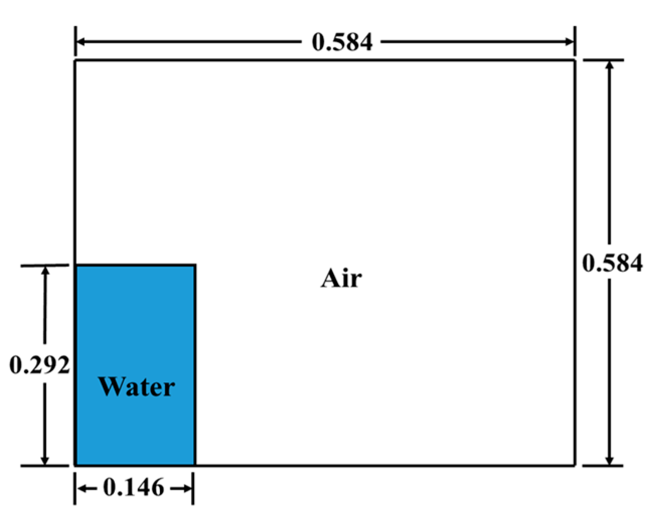
In order to provide sufficient comparison with the model test and verify reliability, the computational model size of the numerical simulation is usually consistent with the size of the model test [49]. Figure 2 illustrates the basic computational formula model for a dam breakdown without any downstream obstacles. The entire calculation domain is a square describer with 0.584 m × 0.584 m. A length of 0.146 m and a height of 0.29 m of static water are provided. The initial state is placed in the lower left corner of container.
3.2. Mesh Division and Boundary Conditions of Foundation Dam Failure Computational Model
The simulations were carried out in the commercial CFD software STAR-CCM+. The geometric model is used to divide the grids. Two-dimensional grids can be circular, quadrilateral, triangular, or polygonal. The quadrilateral grid provides uniform node distribution, a controllable design, a low number of singular points, and a grid edge that is aligned with the edge of the rectangular computing domain. The edge size of the grid is 1.25 mm, the number of grid layers on the rectangular edge is approximately 470, and the total number of two-dimensional grids is about 220,000. There is a slip-free wall surface and a pressure outlet at the top of the rectangular calculation domain’s boundary conditions on the left, right, and bottom. Since the top of the square calculation domain is connected to the atmosphere, the initial pressure of the calculation domain is equal to the atmospheric pressure. The realizable k-ε turbulence model is used. This turbulence model is suitable for a wide range of flow types, including swirling uniform shear flow, free flow (jet and mixing layer), cavity flow, and boundary layer flow. This turbulence model can perform well for dam break simulation with flow separation.
3.3. Data Analysis of Basic Dam Model Calculation Results
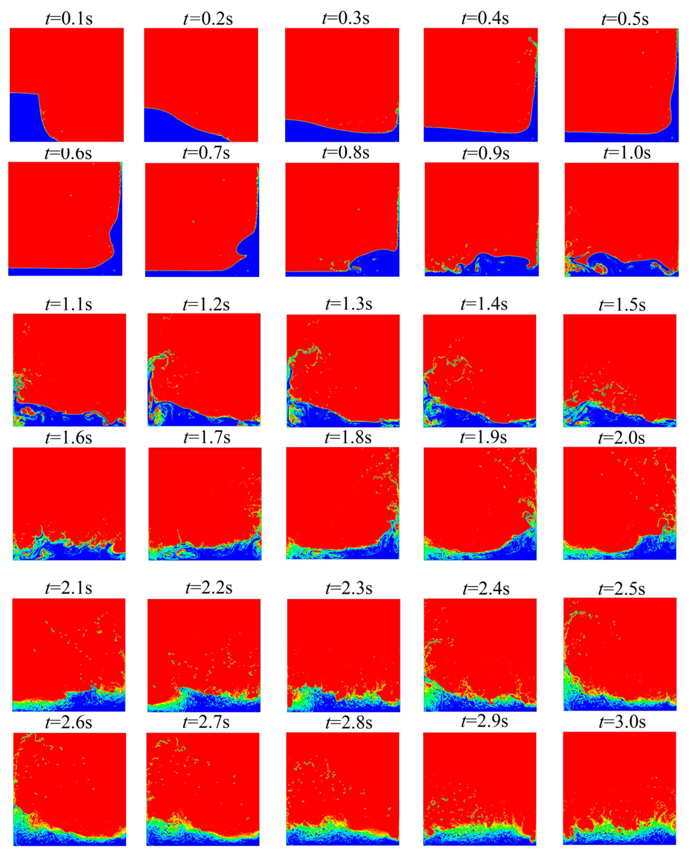
As shown in Figure 3, the dam break process without any obstacles in the downstream can be divided into four stages. First, the water column starts to descend until the front flow hits the right wall of the container. The second phase addresses water flow and the optimum container wall. The interaction of the wall includes inertia backflow and gravity fluid movement up and down the wall. The third stage occurs between the first time the backflow is expelled back to the left wall and the second time it affects the opposite wall of the container. At the fourth stage, gravity and energy loss combine to steady the water flow. The dam breakdown started with the first stage, which is the beginning of the whole process. The water level decreased significantly as the water body changed direction at high speed. The free surface at the top of the water body transforms from a straight line to an arc that arches slightly higher because the water flow on the far right in contact with the air falls quicker than the water flow near to the wall. The rightmost end of the water column forms a long downward curving arc-shaped free surface as the upstream water body squeezes towards the downstream water body under the influence of gravity. The arc-shaped free surface will gradually straighten throughout the water body’s sinking process. The right wall of the rectangular container is reached by the front end of fast-moving water at about t = 0.25 s, and it is brutally struck by the wall before climbing upward. All of this dam breaking activity simultaneously advances to its second stage.
As the water flow rose up the wall in the second stage of dam break, water droplets continued to fall from the front end of the flow. At t = 0.5 s, the speed of water flow climbing along the wall gradually decreases to zero, and then falls and rolls rapidly under the action of gravity. Droplets of water hit with the top of the water as it flows to the right from the bottom, generating a wide variety of bubble sizes and shapes. At the same time, the impact causes a water flow to expel to the left from the area at which bottom water surface and falling water body interact directly. This is the initial water flow on the bottom water surface. Water particles travelling to the right near the bottom of the container caused a second hydraulic leap before hitting the wall, reducing the height. During the process of water flow forming, water droplets keep breaking off and falling back into the water flow. The left wall of container is hit by water flow as it rotates and accelerates to the left. As a result of gravity and the dissipation of kinetic energy, the level of water increases. The water droplets coming out of the increasing water flow become increasingly larger when it strikes the left wall of the container.
During the short period of hitting the right wall, the downstream water body close to the left wall produces a gyrating motion. It will increase the kinetic energy loss of the water flow, thereby greatly reducing the speed of the water flow. It is noteworthy that the second stage of the dam break began near the bottom of the trough after the initial hydraulic surge. In the water container, a substantial air bubble was deformed by extrusion of surrounding flowing water. The air bubble will gradually burst until water returns to the right wall of container. A number of air bubbles of varying sizes develop when the air rushes into the water above as the ascending water falls back below. After switching direction, the water forces the downstream water particles to travel towards the container’s right wall, where it eventually arrives at t = 1.7 s. Here, the process of a dam breaking has reached its third stage. The water body loses energy as it repeatedly collides with the right wall of the container, demonstrating the immense effect of gravity. Nevertheless, compared to the first two stages, both the height of leap and the flow rate of backflow are much reduced. The water body could still climb up the wall and produce backflow. The water flow would continue to wobble left and right throughout the time interval between t = 1.7 s and t = 3 s owing to inertia, but it will finally settle due to energy loss caused by the wall hit.
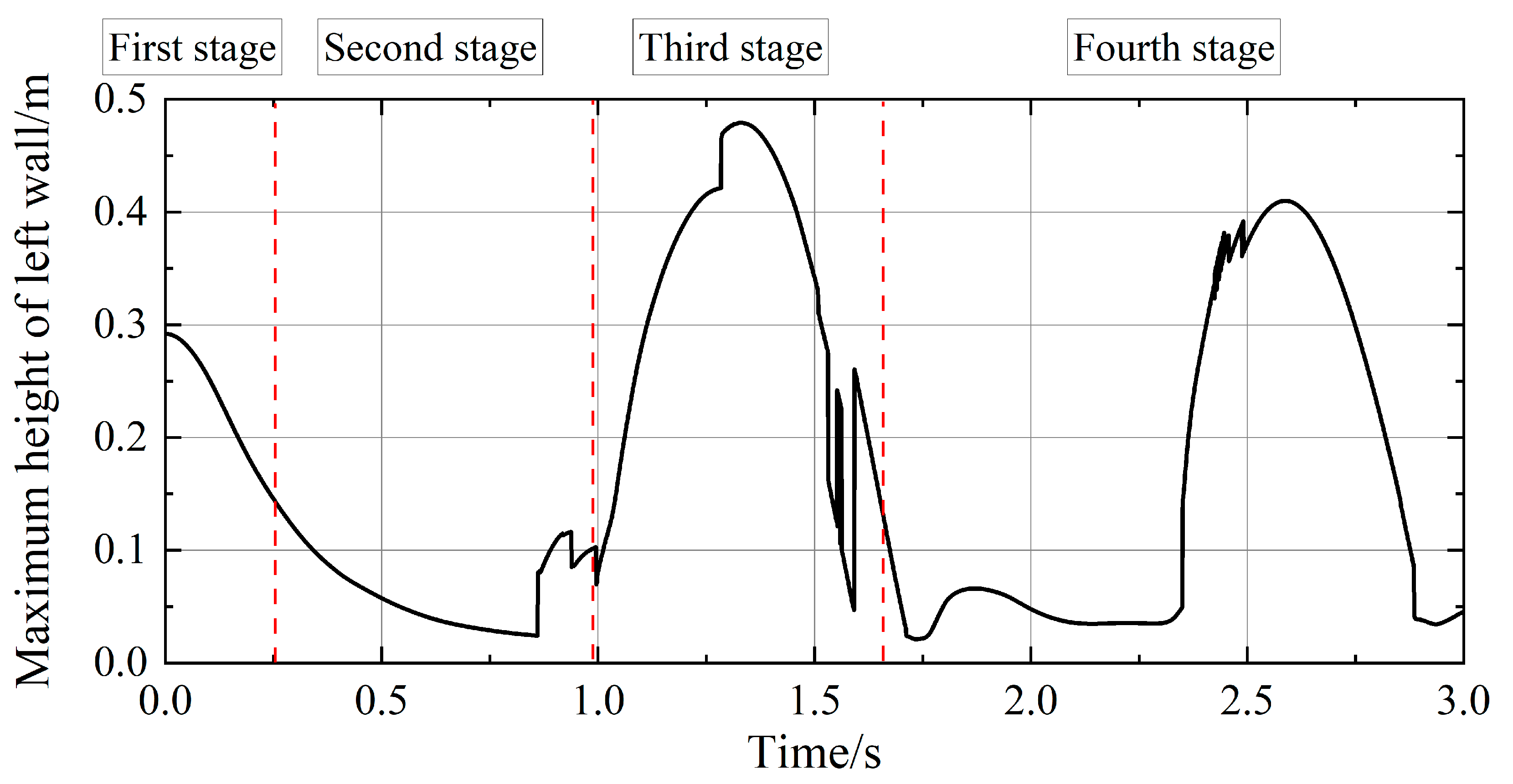
Figure 4 depicts a time series of water level as seen against the left wall of the container. During the first stage of the dam breakdown, the water column height along the left side of the container decreases significantly, and the rate at which it falls grows steadily until it reaches a maximum. When compared with Figure 4, it is obvious that at t = 0.25 s, the leading edge of the water flow has reached the right wall of the container, and the rate of descent of the water column has slowed considerably.
When t = 0.85 s, the separation beads which are formed during the water reflux process will cause the water column on the left side of the container to increase slightly. At time t = 1.0 s, the body of reflux water has reached the left container wall. The height of the free surface on the left wall went through a process of rapid rise at time interval t = 1.0~1.5 s. At the end of the third stage of a dam breaking, there is a repeated jump in the height of the free surface of the left wall. Water droplets that fall off the front of the climbing water flow and adhere to the left wall cause this. The water body returns to the left wall of the container during the shaking process, and the height of the free surface of the left wall gradually varies over a lengthy period thereafter. As compared to the initial return, the maximum height of the free surface is lower because of gravity and energy loss. It is foreseeable that over time, the maximum height of free surface of left wall will continue to decrease until it remains at a fixed height.
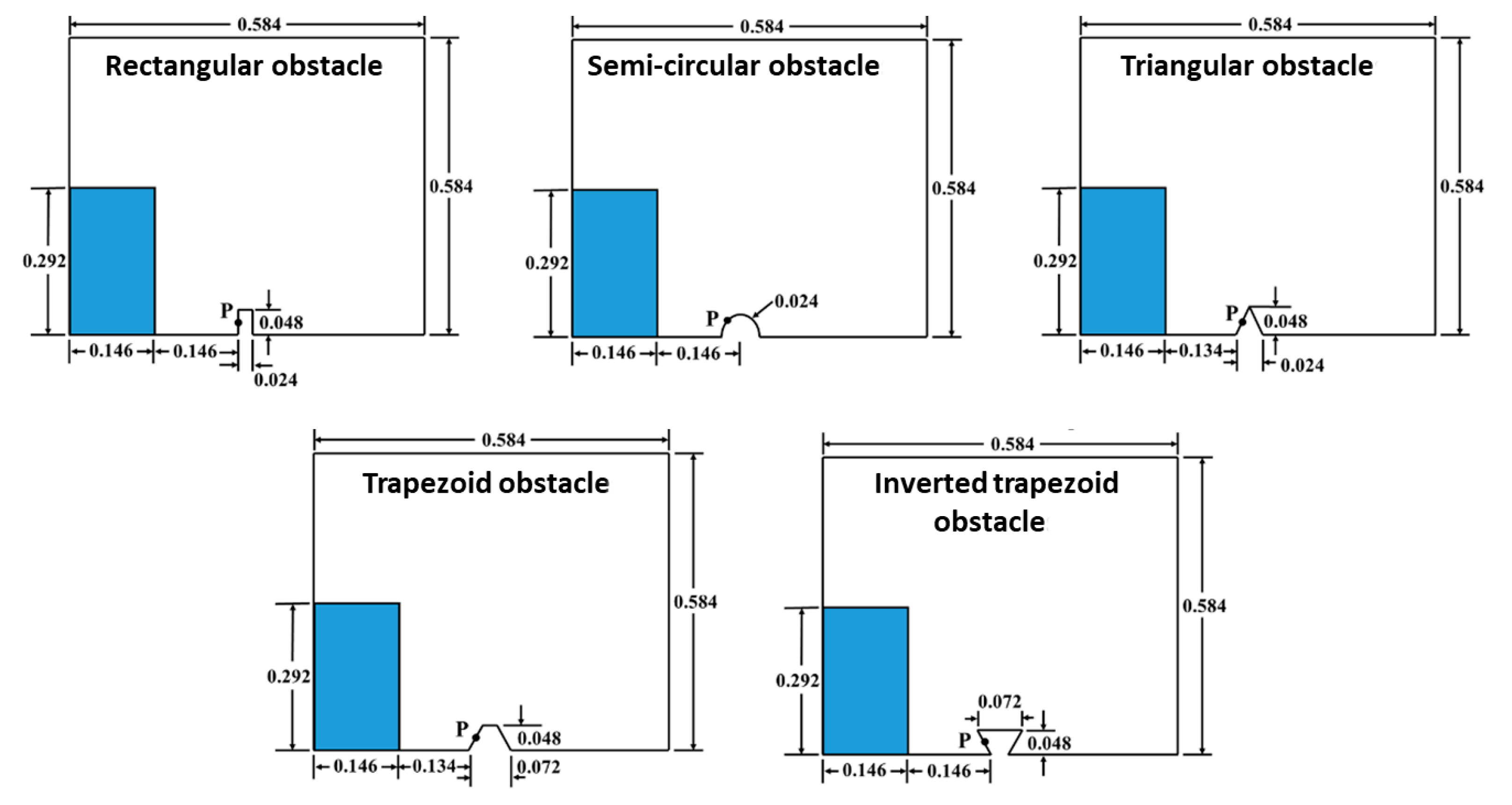
3.4. Comparative Analysis of Dam Failure Models with Diverse Obstacles Shapes Down-Stream
This section compares and contrasts five different calculating models, including the rectangle, semicircle, triangle, trapezoid, and inverted trapezoid. These obstacles can be reflected in buildings downstream of the dam, such as residential buildings, embankments, seawalls, and cofferdams. In order to provide an accurate comparison of various shaped barriers affect dam break flows, it is important that the length and size of each obstruction be as similar as possible. Similarly, a half-side test point P near the water flow could be applied to track variations in pressure that are indicative of the presence of an obstruction. Figure 5 shows calculation models for the breakdown of a dam with five obstacles.
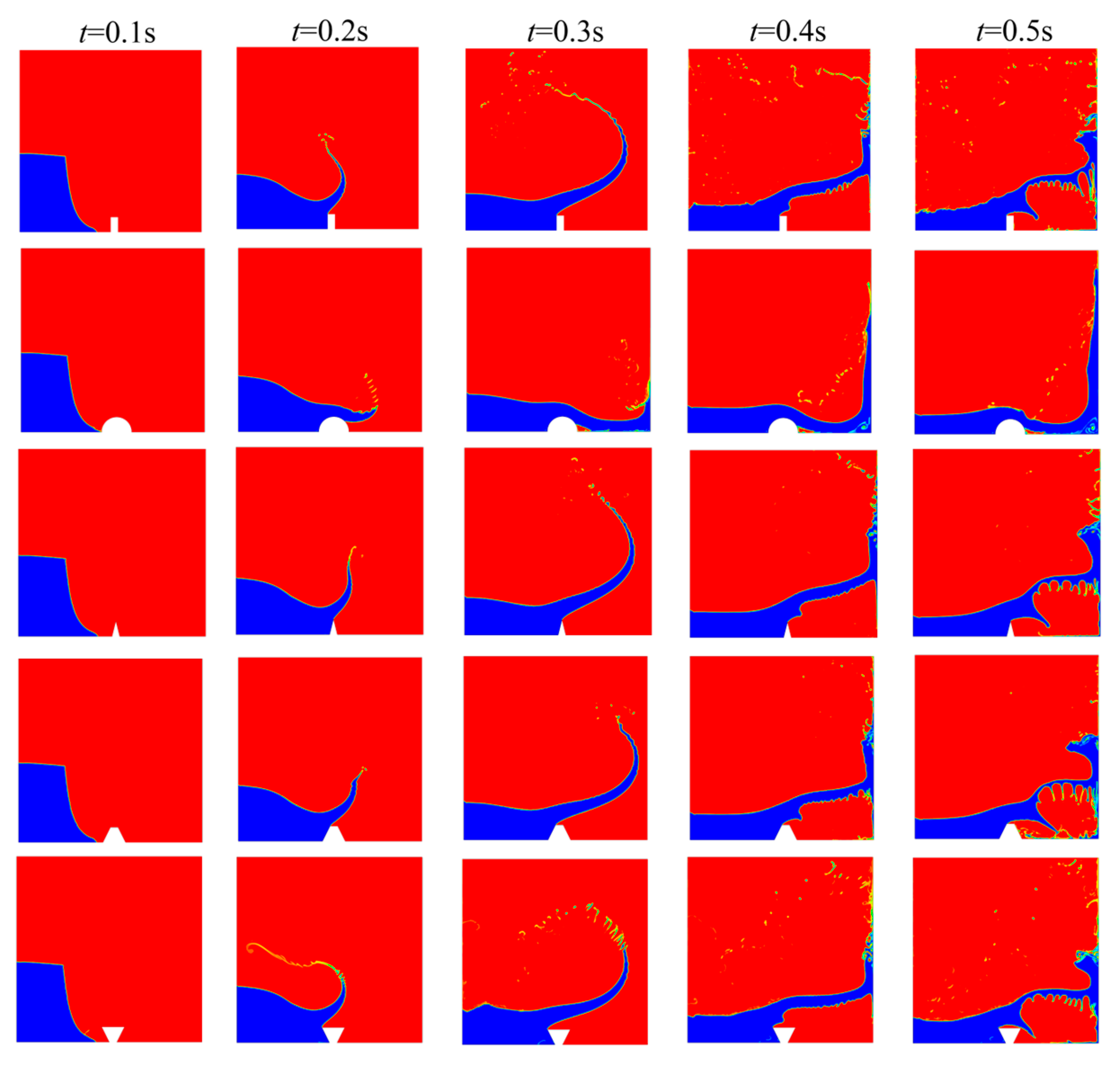
Figure 6 shows that, between 0.1 s to 0.5 s, all except the dam breach with a semicircular obstruction downstream have very similar water flow transformation. The front of the water flow reaches the obstruction at t = 0.2 s, and the front of dam breakwater flow reaches it prior to that time. All of dam breakwaters in the other four models, with the exception of the semicircular barrier, make contact with the water before turning upward and right, generating a water tongue. The shape and size of water tongue, as well as the angle formed with horizontal plane, are determined by height and slope of barrier walls. Both the triangular and trapezoidal obstacles have sidewalls that slope towards the horizontal plane. This reduces the effect of water flow on the obstacle, so the height and size of the water tongue produced by the triangular and trapezoidal obstacles are not as good as that produced by the rectangular obstacle. The direction of the sidewall of an inverted trapezoid is opposite that of a triangle and a regular trapezoid. The sidewall squeezes the advancing water flow, forcing the front water to go backwards and join with the rear water. In contrast to the preceding four obstacles, the front end of water flow does not create a water tongue in front of circular obstacles. After the fore-flow has climbed the left wall, a closed air is generated at the bottom of the right side of circular barrier owing to the flow separation area. The fronts of four different kinds of obstacles that comprise of a water tongue all have an angular region with a convex edge or a sharp point, as can be seen by combining the forms of five different obstacles. If a river flows into this sharp bend, the water will be separated into two separate streams. Whereas water will flow easily from the top of the semicircular obstruction to the downstream, since there are no sharp points in its arc-shaped structure.
Figure 7 shows the free surface flow field of obstacles of different shapes at 0.6–1.0 s, at t = 0.3 s, the water tongues of four obstacles continued to move towards the top right, making an elongated crescent-shaped water whip. Simultaneously, water droplets continue to emerge from the front of the water flow. At t = 0.4 s, the water whip collides with the container’s right wall. At the instant of impact, there is insufficient time for air to disperse, resulting in the formation of bubbles of varying sizes in the water. Under the influence of gravity, the water begins to flow down the right container wall. The air bubbles disperse and spread out as the water flows below. Simultaneously, dispersed water droplets separate from the base of the water whip. A strip of water breaks from the water whip above the obstruction and spills out at the same instant the water whip hits the right wall of the container. At time t = 0.5 s, the water body descends and collides from the right wall to the bottom of the container, causing water droplets to splash. The bulk of the water body on the water whip is driven onto the right wall of container by rear water body. The backwater body continues to contact the right wall of container, increasing the amount of air bubbles in water body. A portion of the water that collides with the right wall of the container falls down along the right wall, while the remainder rushes towards the obstruction. The flow condition of water body with semicircular obstruction at time t = 0.1~0.5 s is comparable to the flow state in Figure 3. The front part of the water body bypasses the semicircular obstacle and then climbs up along the right wall of container.
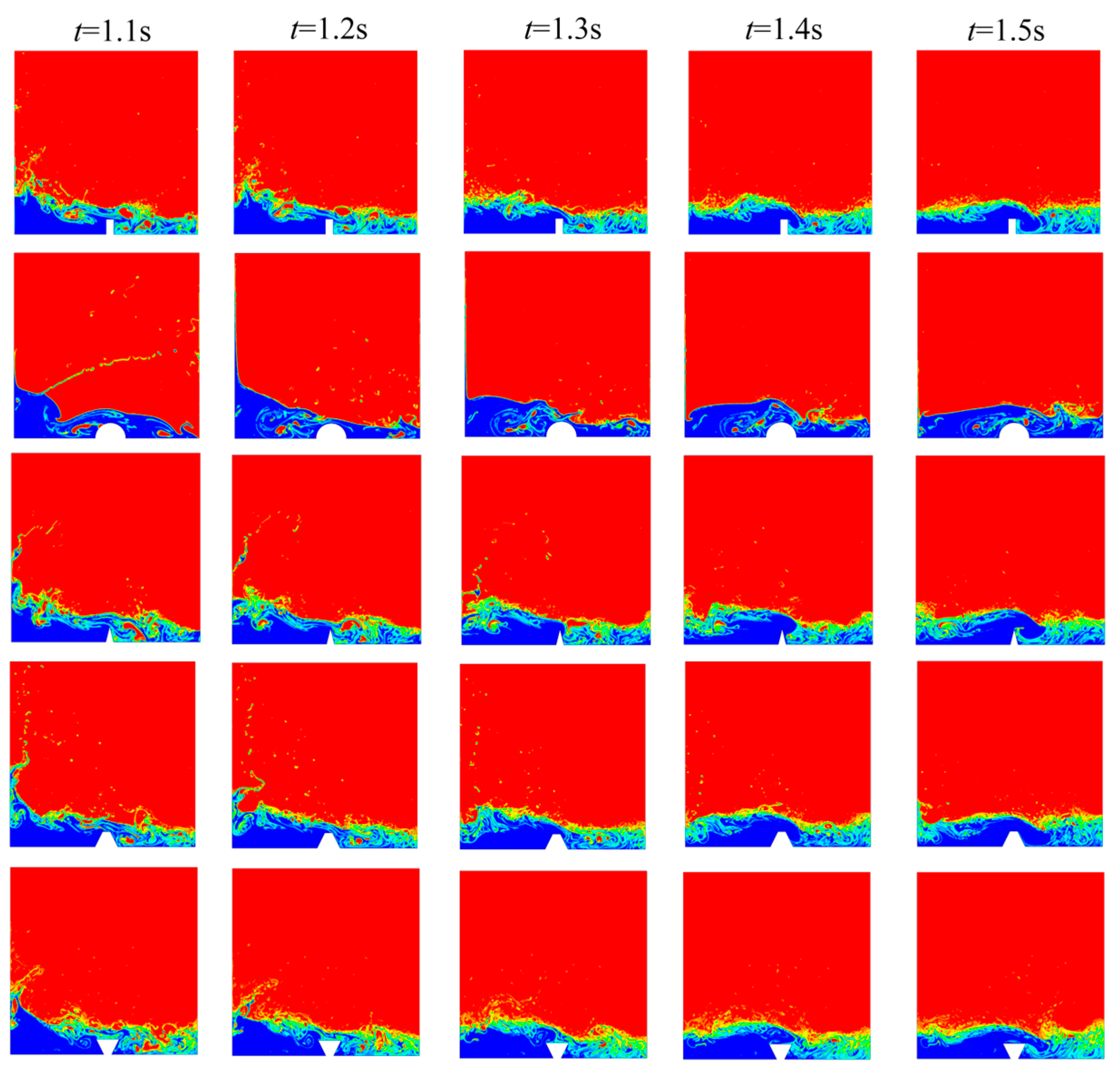
Between t = 0.6–1.0 s, the dam break water flow of barriers of various forms on the right side of the container becomes chaotic and disorganized. The backwater body repeatedly crosses impediment and collides with right wall of the container, splashing forth several water droplets. After being slapped on the top plane of the obstacle, the water body that falls from the right wall and flows to the obstruction will roll and flow back to the left wall. The force-bearing area of a triangle obstruction is a cusp, which theoretically has the minimum interaction force with the water flow. The rectangle and trapezoid have the same top area; hence, their free surface flow changes are identical. The inverted trapezoid has the maximum force-bearing surface and the lowest water body rise. The arc-shaped design of semicircular barriers prevents the water from breaking as rapidly as the prior obstacles, and most of water flows over slightly because of the obstacle.
Figure 8 and Figure 9 show the time between the initial return to the left wall and the second arrival on the right wall owing to downstream obstructions. Compared to when there are no obstacles, the frequency of water spill is substantially lower. While the free surface deforms extremely forcefully in the right region of container during the first 1 s of water flow contact with the obstacle, the flow of the water body is smoother after being hindered by the obstruction, and energy is continually released throughout the impact of water flow with the obstacle.
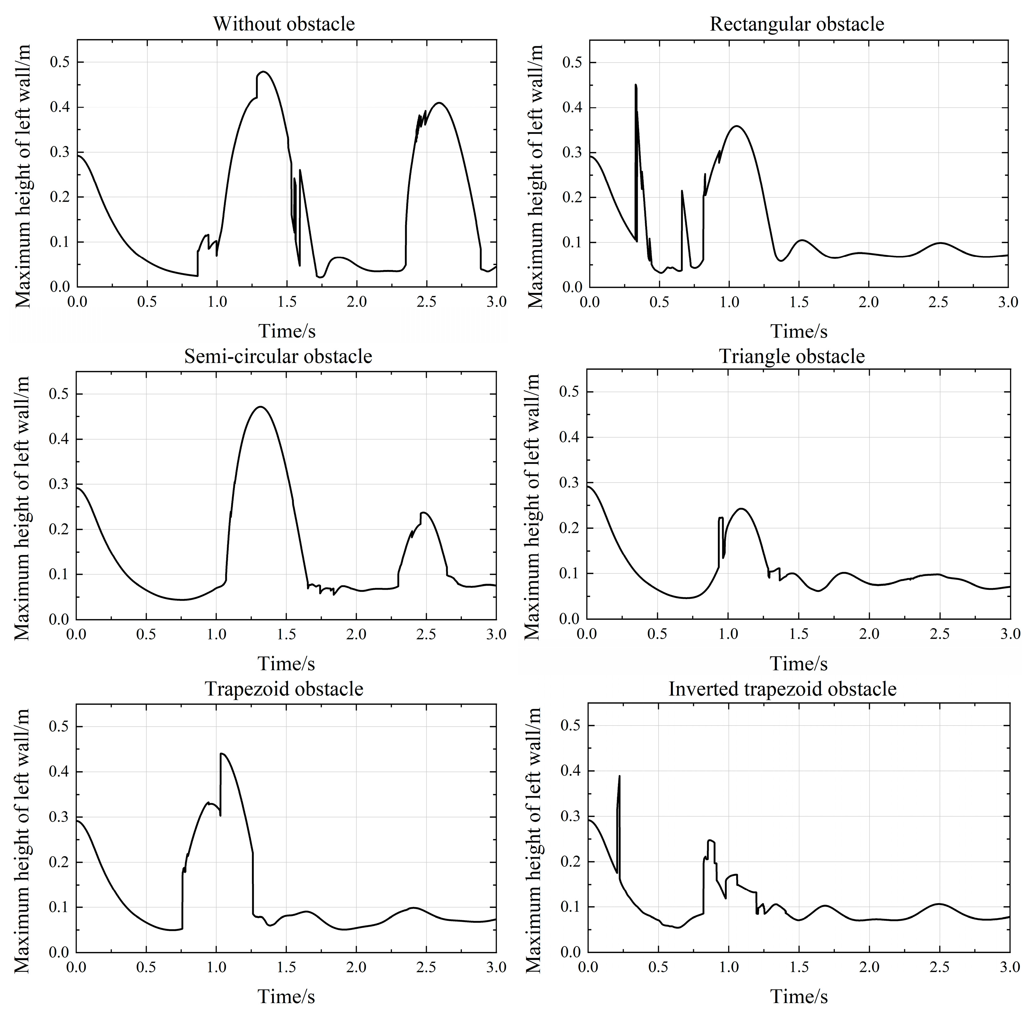
Figure 10 depicts the height of the water column at the left wall of the container with various types of obstructions. Prior to t = 0.5 s, the water flow from the collapse of the dam was falling with a uniform acceleration since the law of height change remained unchanged for each obstacle. The inverted trapezoidal and rectangular obstacles reach their height peak before t = 0.5 s due to water droplets from the front most water flow striking the container’s left wall during the water tongue’s passage. Compared to the rectangular obstacle, the inverted trapezoidal obstacle’s water tongue develops faster and is lower; therefore, its water column’s peak height appears earlier and is smaller.
At t = 0.50–1.25 s, the height of the water column across different-shaped obstacles varied significantly with time. At this stage, the water from the dam does not go back to the left side of the vessel for the first time. For rectangular obstacles, a small portion of the water body created by the water flow hitting the obstacle first flows to the left wall of the container during the process of returning to the left wall, causing an increase in the maximum height of the water column. The value of the maximum height of the water column then increases instantaneously as a significant number of water flows reach the container’s left wall and ascend the wall. The maximum height of water flow rising is decreased by a factor of two when rectangular obstructions are incorporated compared to an unobstructed structure. Of the many different kinds of barriers, the water column height of triangles is minimum in magnitude. Figure 10 shows a thin straight line of water droplets that stay to wall for a shorter duration and increase more rapidly than the total water flow. When the trapezoidal obstacle’s water flow travels to the container’s left wall, a secondary climbing process takes place. The forwards water flow is squeezed by the rear half of the water body during the climb, and the height of the water column rapidly increases to the maximum. With the inverted trapezoidal obstacle at time t = 0.5–1.25 s, the change of maximum height of left wall with time is not parabolic like the other obstacles, but step-like, which indicates that the dam failure return does not directly climb to the left wall. The water droplets separated by dam failure flow repeatedly slap onto wall and attach for a short period, thus forming a step-like height curve. The shape and amplitude of the height curve of the semicircular obstacle at the time interval of t = 0.5–1.25 s are quite similar to the curve of the obstacle, with the exception that there are no leap phenomena at the highest point.
When the dam breaking water flow of the semicircular obstacle moves to about t = 2.3 s, it also climbs slightly on the left wall of the container. The amplitude is half that of when it lacks obstacles, indicating that the semi-circular barriers hamper the water flow very weakly in the first half of the dam break water movement. When the water flow hits the right wall of the container for the first time and goes back to the left wall, it hinders the collapse to some extent of the flow rate of the groundwater. Figure 11 shows that the maximum height of the left wall of the container swings slightly below 0.1 m in the second half, which is consistent with the steady water flow of other obstacles.
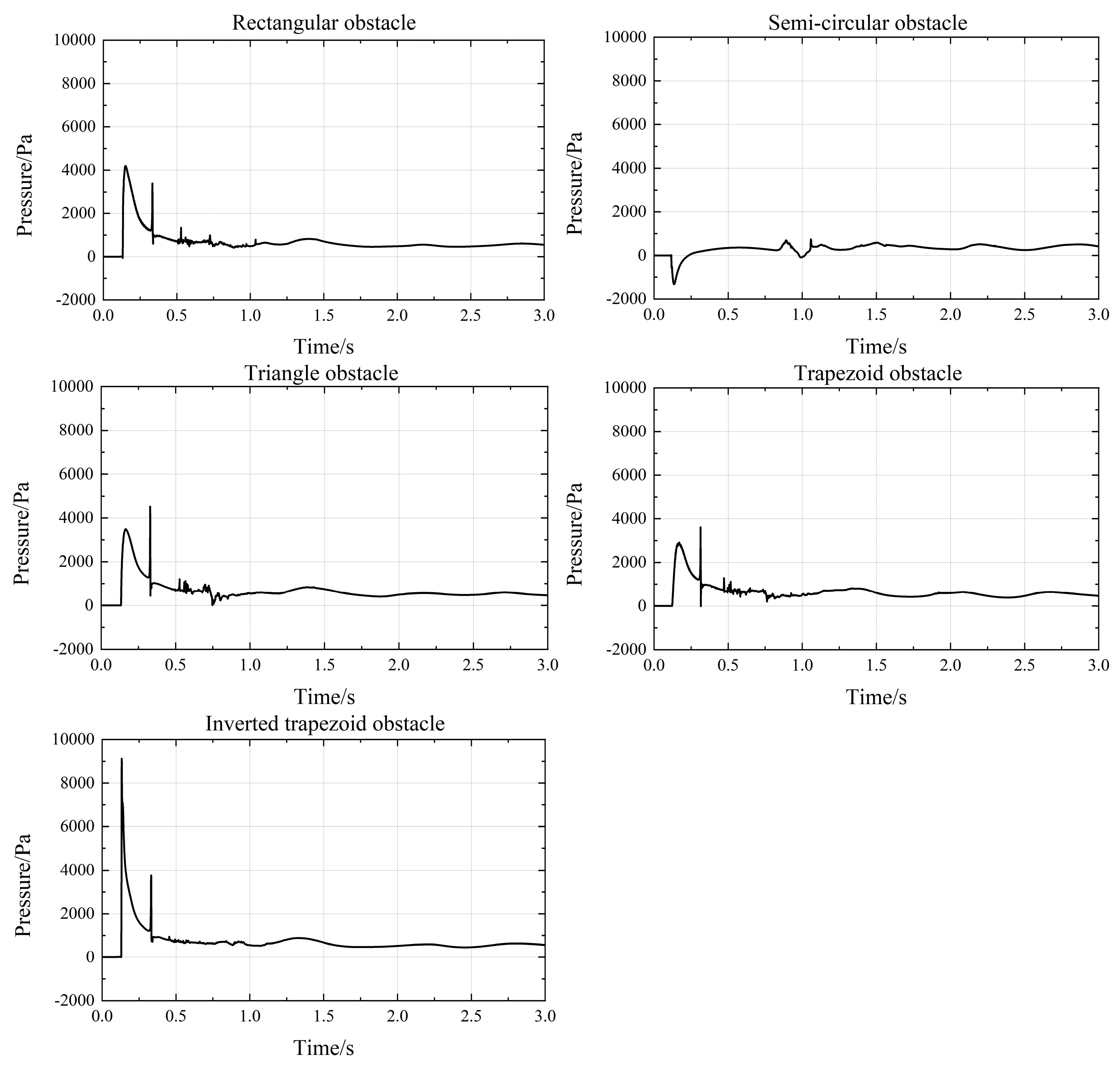
Figure 11 shows a pressure comparison chart for obstacles with various shapes at test point P. The pressure value at test point P varies significantly for flow at 1 s, as seen in Figure 11. The pressure at P of the other four obstacles increases directly as water-flow approaches the obstacle initially, except for the semicircle.
As compared to the rectangle, triangle, and trapezoid, the inverted trapezoidal obstacle increases in pressure significantly more. The influence of water flow is significantly larger on this obstacle than the other three due to the inverted trapezoidal slope. The pressure decreases for semicircular obstructions as water passes through point P. The speed and pressure gradually return to normal when the water passes through point P to the normal flow rate and water pressure values at t = 0.3 s. In combination with Figure 6, we can see that the outer edge of water flow forms a tongue that collides with the right wall of the container. The flow rate stagnated at point P, leading to a rise in the pressure value at this time. The pressure value at point P fluctuates constantly for t = 0.5–1.0 s due to the chaotic water flow. There is no change in the steady rate of water flow after t = 1.0 s, and the pressure value gradually begins to stabilize in its range of variation.
4. Simulation and Analysis of Single Liquid Dam with Wet Bed Downstream
For the dam break water flow problem mentioned above, there is no water flow downstream in the initial state (downstream is a dry bed), and the dam break problem for the initial downstream wet bed situation is one of the current research hotspots [15]. In this section, the dam break experiment with a wet bed downstream carried out by Kocaman and Ozmen-Cagatay [9] in 2015 is used as a calculation model to analyze the influence of downstream water flow on the free surface of dam break.
4.1. Calculation Model of Wet Bed
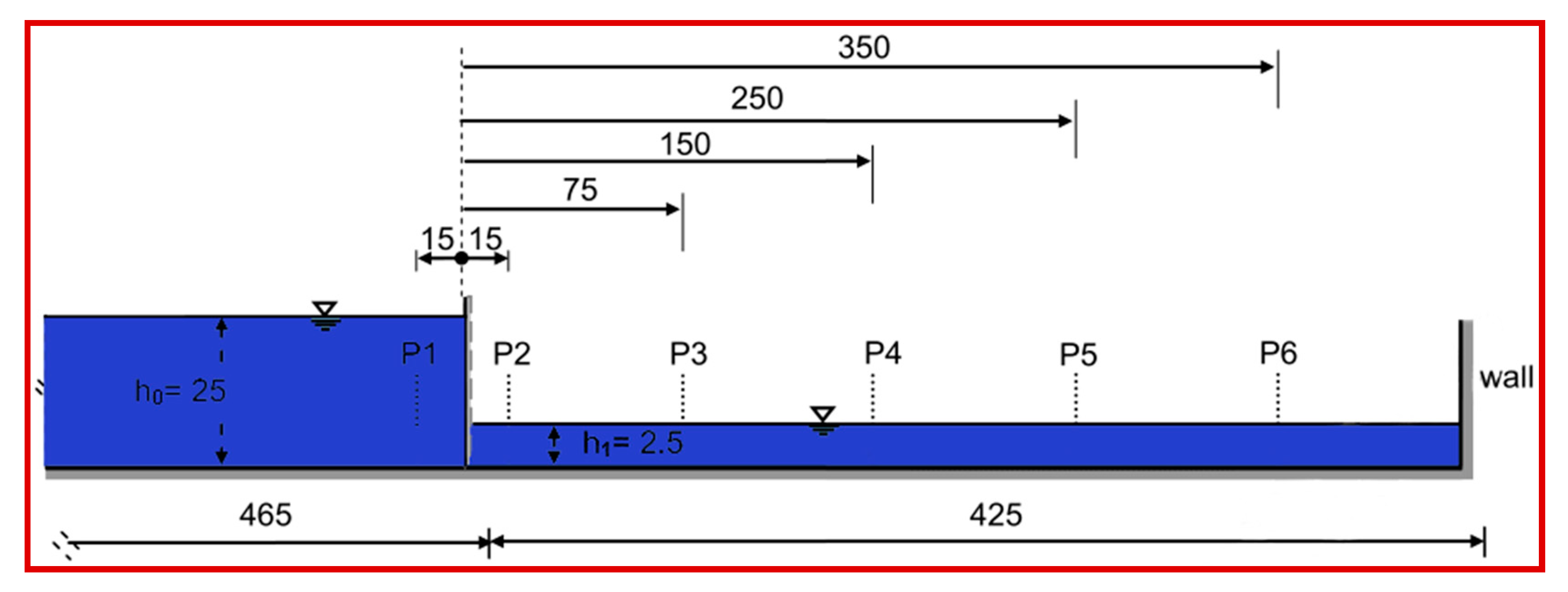
A model of a tank downstream with a wet bed is shown in Figure 12. The upstream water column is 4.65 m long and 0.25 m high, while the downstream water body is 4.25 m long and 0.025 m high. The computational area is 0.5 m high and 8.9 m long. Kocaman’s model test involved the placement of six probes to determine the time-dependent free-surface-height curves of six different cross-sections. Kocaman’s model test maintains the probe at a constant height above the free surface for an extended duration.
4.2. Computational Model of Grid Division with Wet Bed
The number of two-dimensional grids in the downstream calculation domain with wet bed is approximately 100,000. The distribution of an upstream water column and a downstream wet bed in the initial state is shown in Figure 13. Since the top of the tank is connected to the air, the initial pressure of the calculation domain should not be zero but could be equal to the pressure in the atmosphere.
4.3. Distribution and Evolution of Free Surface Flow Field
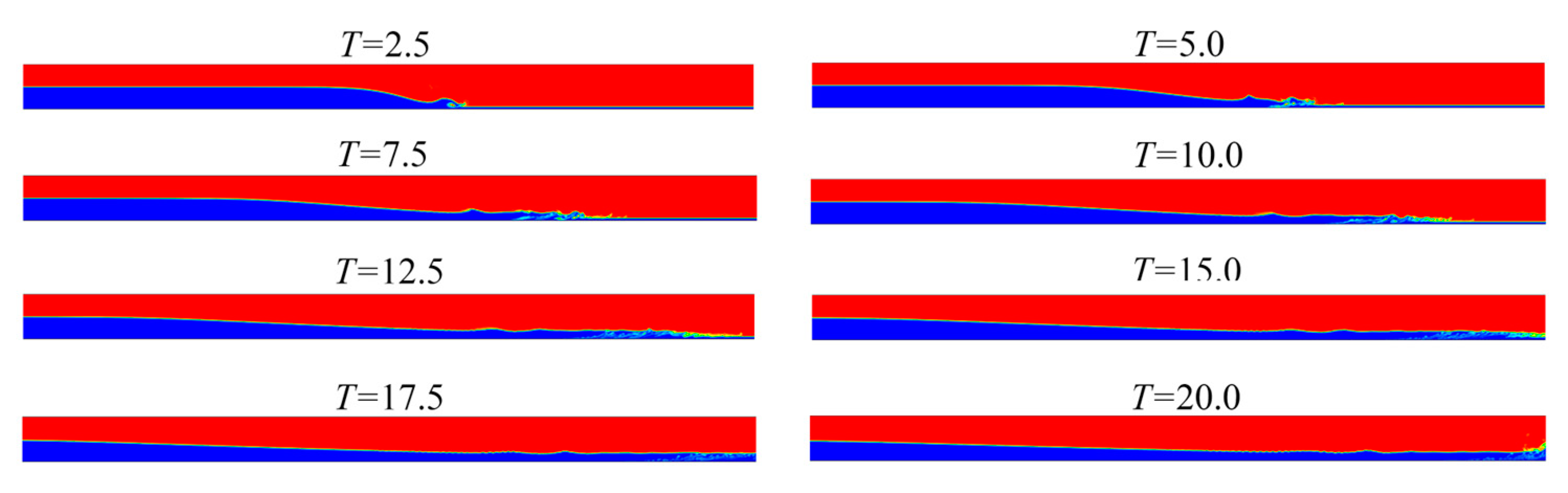
We followed the infinite time T = t(g/h0)0.5, where g is acceleration of gravity, which is 9.81 m/s2. The distribution and evolution of free surface flow field at T = 2.5–80 are shown in Figure 14, Figure 15, Figure 16 and Figure 17. Figure 14 shows that the potential energy of the upstream water is transformed into kinetic energy when the dam breaking water flow begins to move under the effect of gravity. The downstream water may impede the flow of the upstream water when there is 2.5 cm of still water downstream of the flume, causing the upstream water flow to travel upward in the form of a rolling wave.
The wave with the leading edge is broken and a jet forms downstream as a result of an obvious rolling phenomenon at the front end of the dam breaking water flow. The wave breaking on the downstream wet bed during the first stage of the dam break created instability that caused a significant amount of foam development on the wave front before T = 5.0 (physical time 0.79 s). The water flow was mixed with a large amount of air, and after T = 5.0 the air gradually diffuses into the tank while moving with the water flow. During the period of T = 7.5–15.0, the dam break wave moves forward in a waveform similar to a swell after the dam breaks. The dam break wave reaches the right wall of tank at around T = 17.5 (physical time of 2.79 s), is reflected by the wall, and then travels in the direction of the left wall.
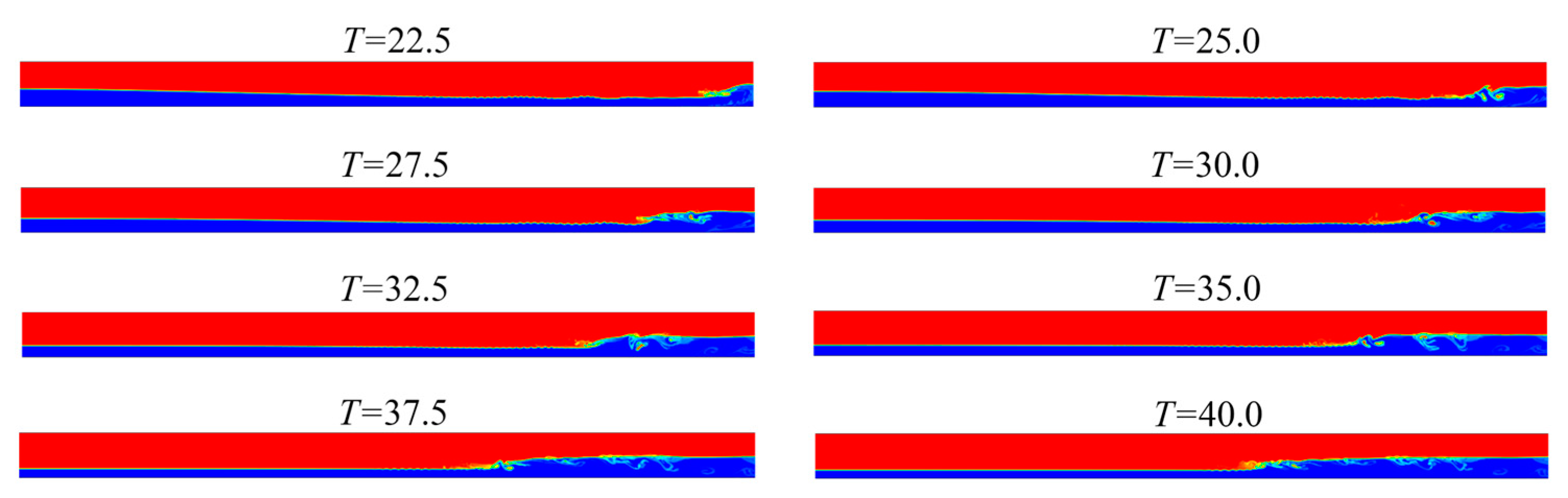
Water surface reflection off the right wall after T = 22.5 results in a leftward-propagating negative wave. The upstream water might flow to the right wall due to a small potential difference in the levels of upstream and downstream water. The wave function speed is decreased due to the mutual interference of the reflected negative and positive waves from the wall. On the open surface of the reflected wave, the turbulence effect brought forth by the early dam wave breaking predominates. As a result, until the breaking wave happens at time T = 35, the front-end peak of the reflected wave becomes sharper (physical time of 5.5 s). After T = 37.5, the water level difference between upstream and downstream gradually becomes zero, and the reflected wave moves gently to the left side of the sink under the action of inertia.
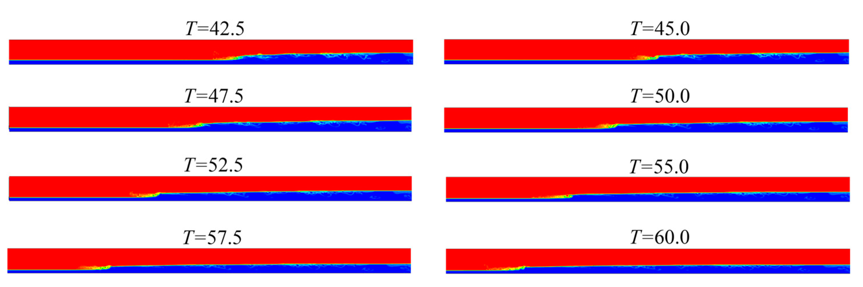
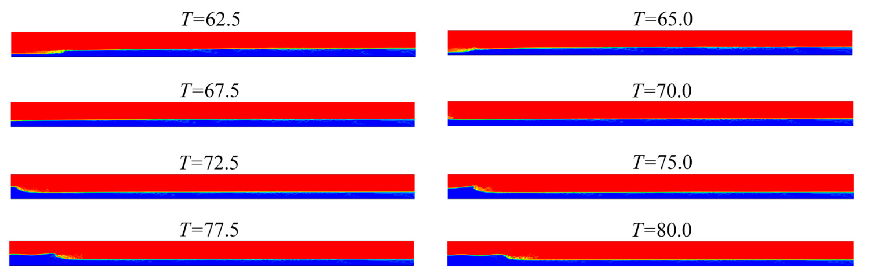
At T = 42.5–80.0, the water wave is a steady sinusoidal waveform that travels from the right side of tank to the left. When the dam wave rebounds and the backflow hits the wall to the left of tank, the front waterbody is slightly compressed by upstream and downstream water bodies. The kinetic energy of return flow reaching the left wall is less than the first time it reaches the right wall, so the degree of rolling of water flow is also greatly reduced.
4.4. Free Surface Height Variation at Different Positions
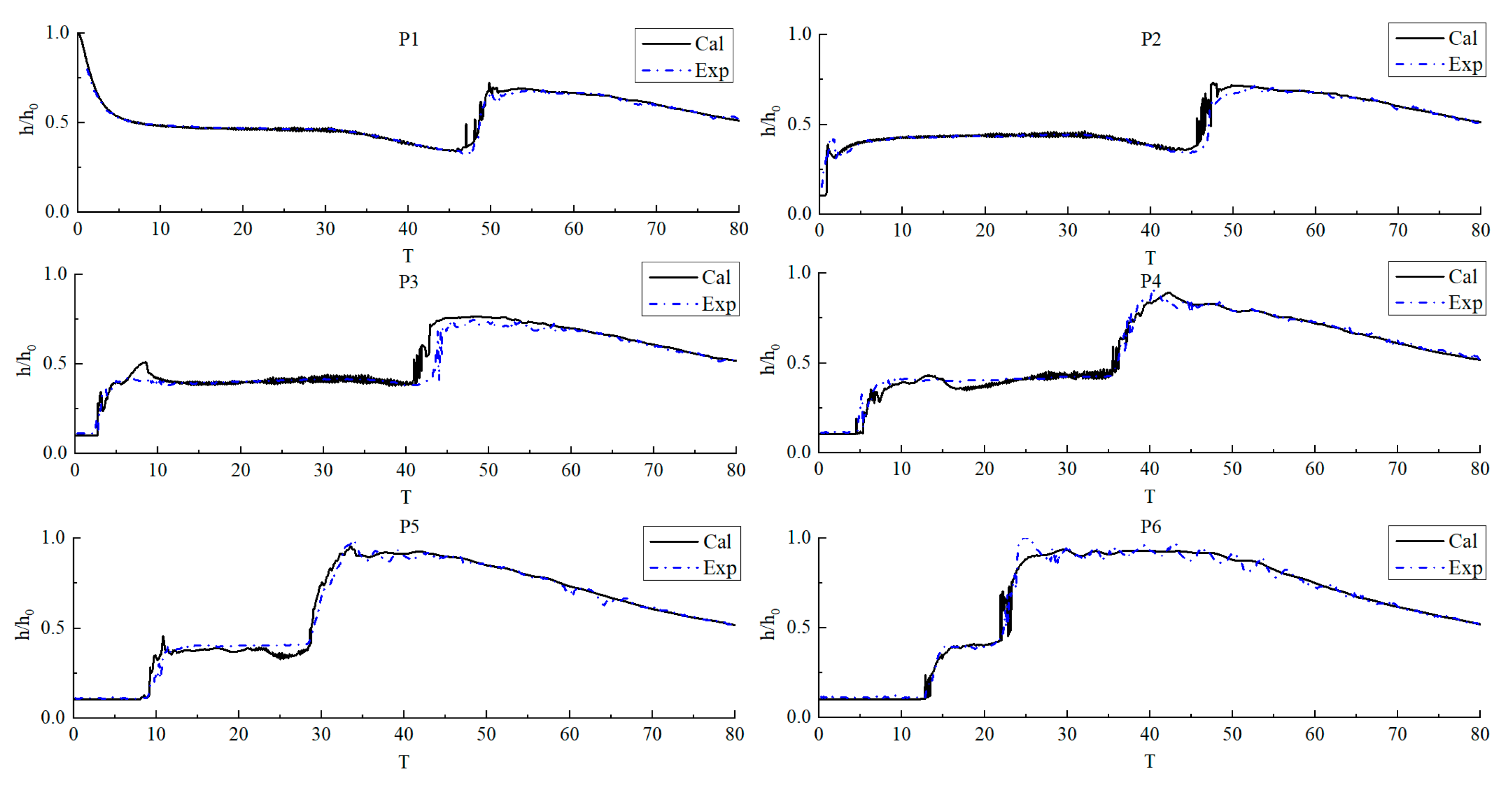
Figure 18 depicts the time-varying curve of water level at six positions. The ordinate represents the ratio of instantaneous height h to the maximum height h0, while the abscissa represents dimensionless time T. In general, the calculated values of water level at the six locations are in good agreement with the experimental values. As the dam break wave reaches the area, the water level at other regions will increase swiftly and remain constant for a long time. The position of P2 is the closest to the upstream water column, so the height of free surface here will rise rapidly after the dam break begins, and then the water level will remain constant before T = 33 and maintain at about h/h0 = 0.43. The water levels of P1 and P2 gradually decreased between T = 32–48 and T = 33–46, respectively, and then rose rapidly to the peak. The second rapid rise in the free surface water level at each location is caused by reflected waves generated by the reflection of the dam break wave against the downstream right wall.
When the moving wave from the dam break hits the wall on the right side of the tank, the wave is reflected, producing a wave with the largest depth. As the reflected wave reaches a height of six positions, it returns to left wall of the tank, triggering a jump in water level. The lag period between the dam break wave and the reflected wave decreases downstream (from P2 to P6) and is smallest at P6. The water level rapidly lowers after the wave is reflected and reaches the upstream end. For P3–P6, the water level remains constant and maintains at h/h0 = 0.40 after the first rapid rise, which indicates that the free surface profile upstream of reflected wave is horizontal. As the dam wave reaches the right wall of the tank, it is reflected and carries on to the measurement section, producing wave columns in all measuring positions. With the passage of time, there is a gradual reduction in the amplitude of the travelling wave. The reflected wave height h/h0 exceeds 1 at P5 and P6, which can be explained by the collision of the reflected wave moving upstream. The dam breaking wave moving downstream results in the superposition and the reflected wave also becomes steeper as it moves upstream.
Typically, insignificant fluctuations with a short wavelength and amplitude emerge on the water’s surface adjacent to the downstream end wall. The reflected wave was first noticed on the portion between points P5 and P6 along the right wall of the downstream stream. At the position near the right wall of the downstream flume (positions P5 and P6), the reflected wave was observed earlier than at other sections. The dam break wave moves from P2 to P5 in 9.5 s, while the reflected wave returns to P2 in 19 s. The right wall of the tank is therefore reached by the dam break wave. When the wave hits the right wall at the rear, some of the energy is lost, decelerating the flow of water by about 50%.
5. Simulation and Analysis of Single Liquid Dam Failure during Gate Twitching
5.1. Dam Breaking Model When the Gate Twitches
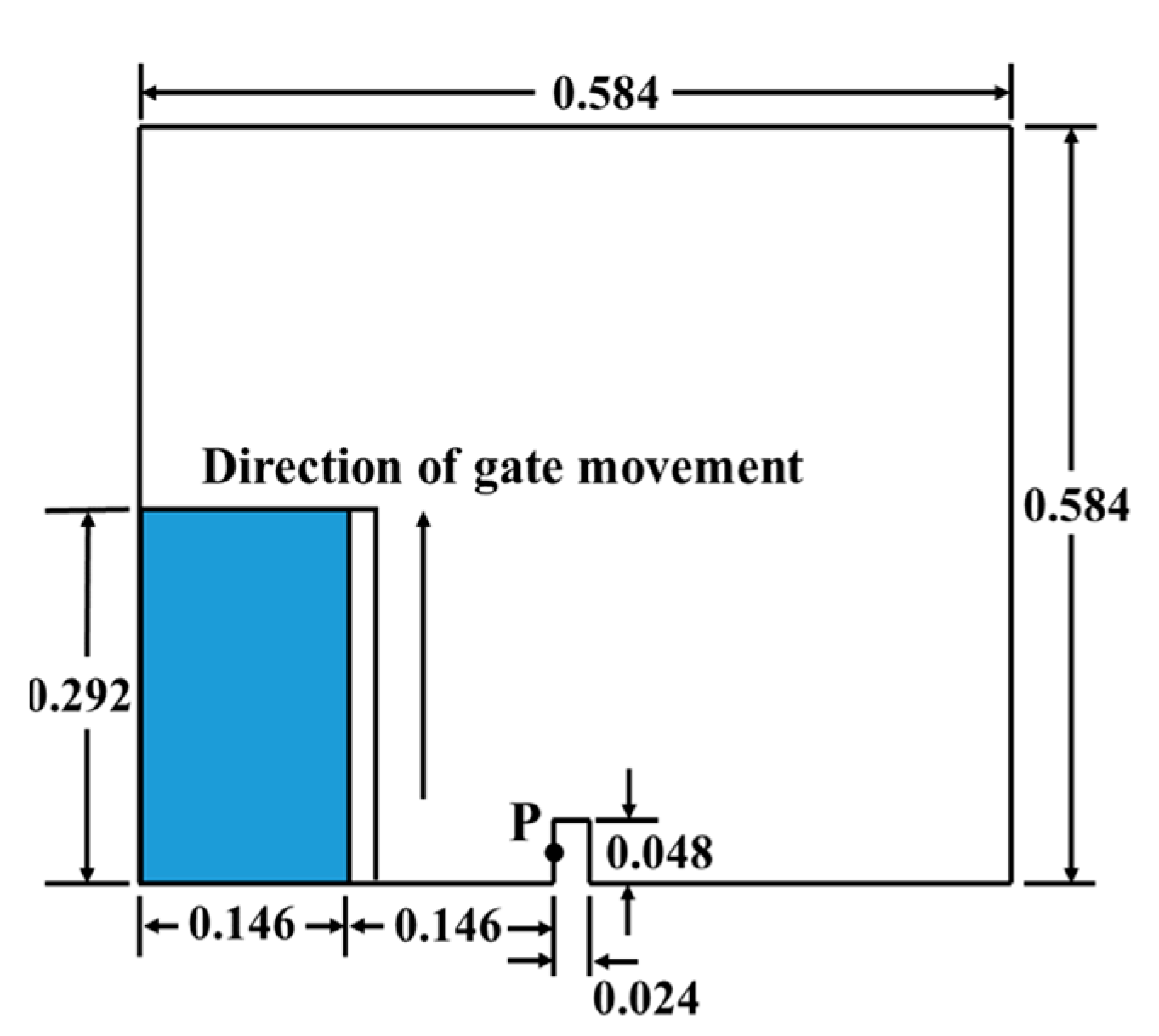
This section takes the dam failure model with rectangular obstacles downstream as an example when the gate twitches, and briefly compares the influence of gate twitching on the flow area of free surface of dam breaking. The dam failure calculation model with gates is shown in Figure 19. The movement speed of the gates is 0.14 m/s, which is realized by the translational movement of overlapping grids. The number of grids in the overlapping domain is 3450, and the number of grids in the background domain is about 85,000.
5.2. Free Surface Flow Field Distribution
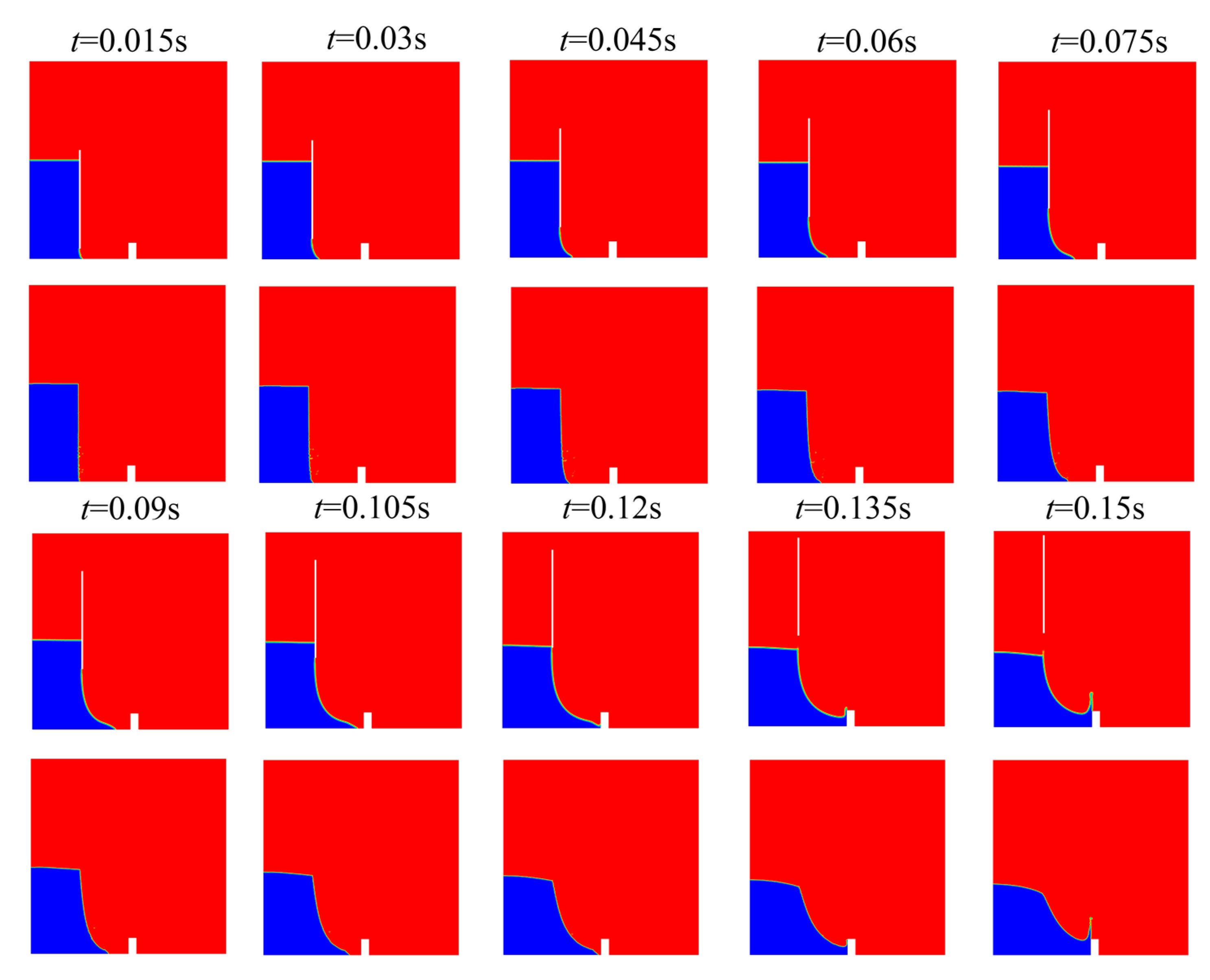
The impact of gates on water flow of dam breaking is mainly concentrated in the process of gate pumping. When the gate is separated from the water flow, it is suspended on the upper left of the container. At this time, there is almost no interaction between the gate and the water flow. When the calculation time is greater than 0.14 s, the translational motion speed of gate is 0, so this section selects the free surface of dam break before 0.15 s as the analysis object. Figure 20 shows that the open surface of the water body upstream of the water column in contact with the sluice gate is relatively fixed at the commencement of dam collapse due to the extrusion limitation. The shape of the free surface hardly changes during the collapse of the water column. The free surface at upper end of water body always maintains a straight shape before the gate leaves the water body and does not form an arched arc. When the gate leaves the water body, the water body is not in any restricted contact with the outside air. The free surface at the far-right end of the water column is affected by the sudden increase in static pressure to form a more curved arc.
During the translational movement of the gate, relative slippage occurs between the water body and the gate. The gate has an upward effect on the water flow, and it reduces fluid velocity of the water body as it encounters it. As the gate moves, a portion of the lower water body is released causing the dam flow to reach the rectangular obstruction sooner. After the gate stops moving, splashes of water during the dam failure occasionally lap on the gate, but the suspended gate does not have a large impact on the subsequent stages of the dam breaking.
6. Conclusions
The simulation results of a single liquid dam breaking with various barriers downstream indicate that the slope at the corner of the obstruction is directly connected to the flow separation phenomenon of the water body. While creating an inverted trapezoidal obstruction, its structural strength should be considered. Triangles and trapezoids generate lower pressure than other obstacles, but their complex shape may impede the construction method. The semicircular blockage causes the least amount of pressure change and has a minor effect on the dam breakdown flow obstruction. In general, rectangular barriers are used for preventing the spread of floodwaters caused by dam breaks.
The simulation results of a single liquid dam collapse with a wet bed downstream indicate that the downstream water would hinder the upstream water flow, causing the upstream water flow to travel upward in a similar form to the sweeping wave. A substantial curling phenomenon occurs at the front end of the dam failure flow, destroying the wave front edge and forming a jet downstream. The water body is in unrestricted contact with the outside air when the gate departs, according to modelling findings of a single liquid dam collapse while the pump is running. The abrupt increase in static pressure causes the free surface at the far-right edge of the water column to bend significantly. The water body and gate fall during gate translation. The gate could be damaged by a few splashing droplets of water during the groundwater breakdown. However, after it begins to flow, the suspended gate will have little impact on subsequent phases.
The present study only considers dam breaks with a single liquid. Future research will focus on the multi-fluid dam break simulation and calculations with the water in the lower stand and the elements of the structure.
Author Contributions
Conceptualization, Z.D. and B.Z.; methodology, B.Z. and Z.D.; software, B.Z.; validation, Z.D. and B.Z.; formal analysis, K.Z. and Z.D.; investigation, H.J. and Z.D.; resources, Z.D.; data curation, B.Z.; writing-original draft preparation, Z.D.; writing-review and editing, B.Z.; visualization, B.Z.; supervision, Z.D.; funding acquisition, Z.D. and H.J. All authors have read and agreed to the published version of the manuscript.
Funding
This research was funded by the Program for Scientific Research Start-up Funds of Guangdong Ocean University, grant number 060302072101, Zhanjiang Marine Youth Talent Project- Comparative Study and Optimization of Horizontal Lifting of Subsea Pipeline, grant number 2021E501.
Data Availability Statement
Not applicable.
Conflicts of Interest
The authors declare no conflict of interest.
References
- Shuang, W.U. Statistics and Analysis of Dam Failures in United States since 2010. Dam Saf. 2020, 5, 61. [Google Scholar]
- Li, H.E.; Sheng, J.B.; He, Y.J. Global dam break events raise an alert about dam safety management. China Water Res. 2020, 16, 19–22+30. (In Chinese) [Google Scholar]
- Xie, J.B.; Sun, D.Y. Statistics of dam failures in China and analysis on failure causations. Water Resou. Hydro. Eng. 2009, 40, 124–128. [Google Scholar]
- You, L.; Li, C.; Min, X.; Xiaolei, T. Review of dam-break research of earth-rock dam combining with dam safety management. Proc. Eng. 2012, 28, 382–388. [Google Scholar] [CrossRef]
- Huang, B.; Ge, L.; Xu, X.; Wang, Y. Application of HEC-RAS in 2D Dam Break Simulation—A Case Study of Hongqi Reservoir. Pearl River 2021, 42, 73–79. (In Chinese) [Google Scholar]
- Yilmaz, A.; Kocaman, S.; Demirci, M. Numerical Modeling of the Dam-Break Wave Impact on Elastic Sluice Gate: A New Benchmark Case for Hydroelasticity Problems. Ocean Eng. 2021, 231, 108870. [Google Scholar] [CrossRef]
- Kocaman, S.; Evangelista, S.; Guzel, H.; Dal, K.; Yilmaz, A.; Viccione, G. Experimental and Numerical Investigation of 3d Dam-Break Wave Propagation in an Enclosed Domain with Dry and Wet Bottom. Appl. Sci. 2021, 11, 5638. [Google Scholar] [CrossRef]
- Kocaman, S.; Dal, K. A New Experimental Study and SPH Comparison for the Sequential Dam-Break Problem. J. Mar. Sci. Eng. 2020, 8, 905. [Google Scholar] [CrossRef]
- Kocaman, S.; Ozmen-Cagatay, H. Investigation of Dam-Break Induced Shock Waves Impact on a Vertical Wall. J. Hydrol. 2015, 525, 1–12. [Google Scholar] [CrossRef]
- Kocaman, S.; Ozmen-Cagatay, H. The Effect of Lateral Channel Contraction on Dam Break Flows: Laboratory Experiment. J. Hydrol. 2012, 432, 145–153. [Google Scholar] [CrossRef]
- Issakhov, A.; Zhandaulet, Y.; Nogaeva, A. Numerical simulation of dam break flow for various forms of the obstacle by VOF method. Int. J. Multi. Flow. 2018, 109, 191–206. [Google Scholar] [CrossRef]
- Issakhov, A.; Imanberdiyeva, M. Numerical simulation of the movement of water surface of dam break flow by VOF methods for various obstacles. Int. J. Heat. Mass. Transfer 2019, 136, 1030–1051. [Google Scholar] [CrossRef]
- Li, Y.L.; Wan, L.; Wang, Y.H.; Ma, C.P.; Ren, L. Numerical investigation of interface capturing method by the Rayleigh-Taylor instability, dambreak and solitary wave problems. Ocean Eng. 2020, 194, 106583. [Google Scholar] [CrossRef]
- Issakhov, A.; Imanberdiyeva, M. Numerical modelling of the water surface movement with macroscopic particles of dam break flow for various obstacles. J. Hydro. Resour. 2021, 59, 523–544. [Google Scholar] [CrossRef]
- Mokrani, C.; Abadie, S. Conditions for peak pressure stability in VOF simulations of dam break flow impact. J. Fluids Struc. 2016, 62, 86–103. [Google Scholar] [CrossRef]
- Khoshkonesh, A.; Nsom, B.; Bahmanpouri, F.; Dehrashid, F.A.; Adeli, A. Numerical study of the dynamics and structure of a partial dam-break flow using the VOF method. Water Resou. Mana. 2021, 35, 1513–1528. [Google Scholar] [CrossRef]
- Munoz, D.H.; Constantinescu, G. 3-D dam break flow simulations in simplified and complex domains. Adv. Water Resour. 2020, 137, 103510. [Google Scholar] [CrossRef]
- Chang, T.J.; Kao, H.M.; Chang, K.H.; Hsu, M.H. Numerical simulation of shallow-water dam break flows in open channels using smoothed particle hydrodynamics. J. Hydro. 2011, 408, 78–90. [Google Scholar] [CrossRef]
- Xu, X. An improved SPH approach for simulating 3D dam-break flows with breaking waves. Comput. Methods Appl. Mech. Eng. 2016, 311, 723–742. [Google Scholar] [CrossRef]
- Wu, Y.; Tian, L.; Rubinato, M.; Gu, S.; Yu, T.; Xu, Z.; Cao, P.; Wang, X.; Zhao, Q. A New Parallel Framework of SPH-SWE for Dam Break Simulation Based on OpenMP. Water 2020, 12, 1395. [Google Scholar] [CrossRef]
- Soleimani, K.; Ketabdari, M.J. Meshfree modeling of near field two-liquid mixing process in the presence of different obstacles. Ocean Eng. 2020, 213, 107625. [Google Scholar] [CrossRef]
- Gu, Z.H.; Wen, H.L.; Yu, C.-H.; Sheu, T.W. Interface-Preserving Level Set Method for Simulating Dam-Break Flows. J. Comput. Phys. 2018, 374, 249–280. [Google Scholar] [CrossRef]
- Zhang, Y.; Chen, J. Numerical Simulation of 2-D Dambreak Wave by Using Conservation Element and Solution Element Method. J. Hydraul. Eng. 2005, 36, 1224–1229. [Google Scholar]
- Miao, J.; Huang, C.; Zhang, X. Research on Dambreak Flow Simulation by Meshfree SPH Method. C.R. Wat. Hyd. 2012, 01, 134–136. [Google Scholar]
- Xu, X.; Jiang, Y.; Yu, P. SPH simulations of 3D dam-break flow against various forms of the obstacle: Toward an optimal design. Ocean Eng. 2021, 229, 108978. [Google Scholar] [CrossRef]
- Hervouet, J.M. Hydrodynamics of Free Surface Flows: Modelling with the Finite Element Method; John Wiley and Sons: Hoboken, NJ, USA, 2007. [Google Scholar]
- Seyedashraf, O.; Akhtari, A.A. Two-dimensional numerical modeling of dam-break flow using a new TVD finite-element scheme. J. Braz. Soc. Mech. Sci. Eng. 2017, 39, 4393–4401. [Google Scholar] [CrossRef]
- Harlan, D.; Adityawan, M.B.; Natakusumah, D.K.; Zendrato, N.L.H. Application of numerical filter to a Taylor Galerkin finite element model for movable bed dam break flows. GEOMATE J. 2019, 16, 209–216. [Google Scholar] [CrossRef]
- Larese, A.N.T.O.N.I.A.; Rossi, R.; Oñate, E.; Idelsohn, S.R. Validation of the particle finite element method (PFEM) for simulation of free surface flows. Eng. Comput. 2013, 10, 385–425. [Google Scholar] [CrossRef]
- Savant, G.; Berger, C.; McAlpin, T.O.; Tate, J.N. Efficient implicit finite-element hydrodynamic model for dam and levee breach. J. Hydra. Eng. 2011, 137, 1005–1018. [Google Scholar] [CrossRef]
- Zhang, T.; Peng, L.; Feng, P. Evaluation of a 3D unstructured-mesh finite element model for dam-break floods. Comput. Fluids 2018, 160, 64–77. [Google Scholar] [CrossRef]
- Hosseini Boosari, S.S. Predicting the Dynamic Parameters of Multiphase Flow in CFD (Dam-Break Simulation) Using Artificial Intelligence-(Cascading Deployment). Fluids 2019, 4, 44. [Google Scholar] [CrossRef]
- Nourani, V.; Hakimzadeh, H.; Amini, A.B. Implementation of artificial neural network technique in the simulation of dam breach hydrograph. J. Hydro. 2012, 14, 478–496. [Google Scholar] [CrossRef]
- Mu, D.; Chen, L.; Ning, D. Three-D Numerical Study of Interaction between Dam-break Wave and Circular Cylinder. S.C. 2020, 61, 231–239. [Google Scholar]
- Wang, B.; Chen, Y.; Wu, C.; Peng, Y.; Song, J.; Liu, W.; Liu, X. Empirical and semi-analytical models for predicting peak outflows caused by embankment dam failures. J. Hydrol. 2018, 562, 692–702. [Google Scholar] [CrossRef]
- Aureli, F.; Maranzoni, A.; Petaccia, G. Review of historical dam-break events and laboratory tests on real topography for the validation of numerical models. Water-Sui 2021, 13, 1968. [Google Scholar] [CrossRef]
- Li, W.; Zhu, J.; Fu, L.; Zhu, Q.; Guo, Y.; Gong, Y. A rapid 3D reproduction system of dam-break floods constrained by post-disaster information. Environ. Modell. Softw. 2021, 139, 104994. [Google Scholar] [CrossRef]
- Azeez, O.; Elfeki, A.; Kamis, A.S.; Chaabani, A. Dam break analysis and flood disaster simulation in arid urban environment: The Um Al-Khair dam case study, Jeddah, Saudi Arabia. Nat. Hazards 2020, 100, 995–1011. [Google Scholar] [CrossRef]
- Ye, Y.; Xu, T.; Zhu, D.Z. Numerical analysis of dam-break waves propagating over dry and wet beds by the mesh-free method. Ocean Eng. 2020, 217, 107969. [Google Scholar] [CrossRef]
- Bahmanpouri, F.; Daliri, M.; Khoshkonesh, A.; Namin, M.M.; Buccino, M. Bed compaction effect on dam break flow over erodible bed; experimental and numerical modeling. J. Hydrol. 2021, 594, 125645. [Google Scholar] [CrossRef]
- Ahmadi, S.M.; Yamamoto, Y. A New Dam-Break Outflow-Rate Concept and Its Installation to a Hydro-Morphodynamics Simulation Model Based on FDM (An Example on Amagase Dam of Japan). Water 2021, 13, 1759. [Google Scholar] [CrossRef]
- Cai, W.; Zhu, X.; Peng, A.; Wang, X.; Fan, Z. Flood Risk Analysis for Cascade Dam Systems: A Case Study in the Dadu River Basin in China. Water 2019, 11, 1365. [Google Scholar] [CrossRef]
- Cantero-Chinchilla, F.N.; Bergillos, R.J.; Gamero, P.; Castro-Orgaz, O.; Cea, L.; Hager, W.H. Vertically Averaged and Moment Equations for Dam-Break Wave Modeling: Shallow Water Hypotheses. Water 2020, 12, 3232. [Google Scholar] [CrossRef]
- Bello, D.; Alcayaga, H.; Caamaño, D.; Pizarro, A. Influence of Dam Breach Parameter Statistical Definition on Resulting Rupture Maximum Discharge. Water 2022, 14, 1776. [Google Scholar] [CrossRef]
- Issakhov, A.; Zhandaulet, Y. Numerical study of dam break waves on movable beds for various forms of the obstacle by VOF method. Ocean Eng. 2020, 209, 107459. [Google Scholar] [CrossRef]
- Hernández-Fontes, J.V.; Vitola, M.A.; Esperança, P.T.; Sphaier, S.H.; Silva, R. Patterns and vertical loads in water shipping in systematic wet dam-break experiments. Ocean Eng. 2020, 197, 106891. [Google Scholar] [CrossRef]
- Wang, C.N.; Yang, F.C.; Nguyen, V.T.T.; Vo, N.T.M. CFD Analysis and Optimum Design for a Centrifugal Pump Using an Effectively Artificial Intelligent Algorithm. Micromachines 2022, 13, 1208. [Google Scholar] [CrossRef]
- Nguyen, V.T.T.; Vo, T.M.N. Centrifugal Pump Design: An Optimization. Eurasia Procee. Sci. Techn. Engi Math. 2022, 17, 136–151. [Google Scholar] [CrossRef]
- Yao, Z.; Peng, Y. Numerical Simulation of Dam Break Flood and Its Application; China Water & Power Press: Beijing, China, 2013. (In Chinese) [Google Scholar]
Figure 1.
VOF model.

Figure 2.
Dam break foundation calculation model.

Figure 3.
Free surface at typical time in 0~3 s.

Figure 4.
Changes in the height of the water column on the left wall.

Figure 5.
Calculation models of different obstacles.

Figure 6.
The free surface flow field of obstacles of different shapes at 0.1–0.5 s (from top to bottom, it is rectangular, semi-circular, triangular, regular trapezoid and inverted trapezoid).
Figure 6.
The free surface flow field of obstacles of different shapes at 0.1–0.5 s (from top to bottom, it is rectangular, semi-circular, triangular, regular trapezoid and inverted trapezoid).

Figure 7.
The free surface flow field of obstacles of different shapes at 0.6–1.0 s.

Figure 8.
The free surface flow field of obstacles of different shapes at 1.1–1.5 s.

Figure 9.
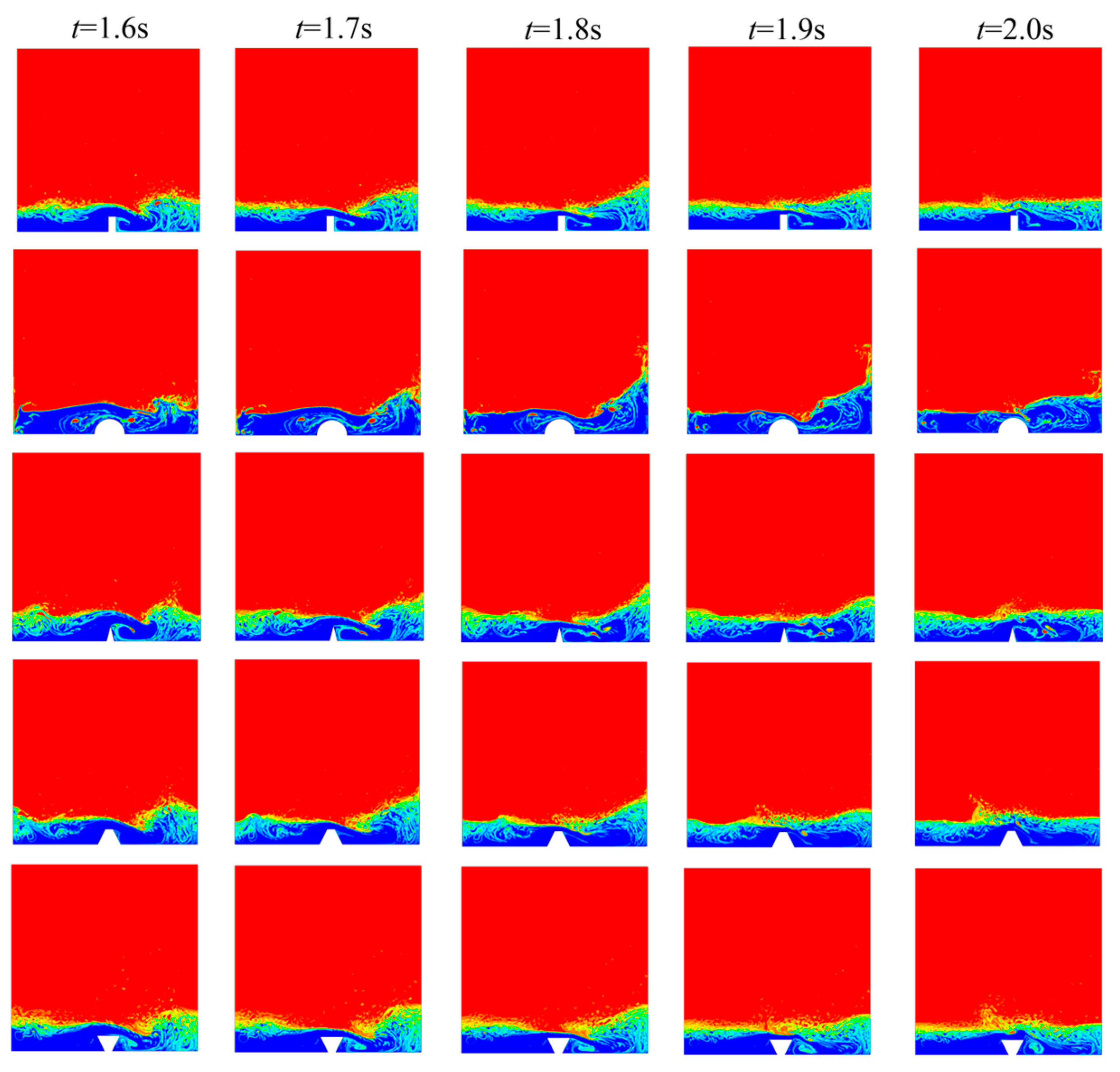
The free surface flow field of obstacles of different shapes at 1.6–2.0 s.

Figure 10.
The maximum height of the water column on the left wall of the obstruction container of different shapes.
Figure 10.
The maximum height of the water column on the left wall of the obstruction container of different shapes.

Figure 11.
Pressure at test points of obstacles with different shapes.

Figure 12.
Calculation model with wet bed.

Figure 13.
Distribution of an upstream water column and a downstream wet bed in the initial state.

Figure 14.
Free surface at T = 2.5~20.0.

Figure 15.
Free surface at T = 22.5–40.0.

Figure 16.
Free surface at T = 42.5–60.0.

Figure 17.
Free surface at T = 62.5–80.0.

Figure 18.
Altitude changes at 6 positions.

Figure 19.
Calculation model with gate.

Figure 20.
Free face comparison with and without gate.

Disclaimer/Publisher’s Note: The statements, opinions and data contained in all publications are solely those of the individual author(s) and contributor(s) and not of MDPI and/or the editor(s). MDPI and/or the editor(s) disclaim responsibility for any injury to people or property resulting from any ideas, methods, instructions or products referred to in the content. |
© 2023 by the authors. Licensee MDPI, Basel, Switzerland. This article is an open access article distributed under the terms and conditions of the Creative Commons Attribution (CC BY) license (https://creativecommons.org/licenses/by/4.0/).
Share and Cite
MDPI and ACS Style
Jiang, H.; Zhao, B.; Dapeng, Z.; Zhu, K. Numerical Simulation of Two-Dimensional Dam Failure and Free-Side Deformation Flow Studies. Water 2023, 15, 1515. https://doi.org/10.3390/w15081515
AMA Style
Jiang H, Zhao B, Dapeng Z, Zhu K. Numerical Simulation of Two-Dimensional Dam Failure and Free-Side Deformation Flow Studies. Water. 2023; 15(8):1515. https://doi.org/10.3390/w15081515
Chicago/Turabian StyleJiang, Haoyu, Bowen Zhao, Zhang Dapeng, and Keqiang Zhu. 2023. "Numerical Simulation of Two-Dimensional Dam Failure and Free-Side Deformation Flow Studies" Water 15, no. 8: 1515. https://doi.org/10.3390/w15081515
Note that from the first issue of 2016, this journal uses article numbers instead of page numbers. See further details here.