Article

Linear and Non-Linear Modelling of Bromate Formation during Ozonation of Surface Water in Drinking Water Production

1
Faculty of Food Technology and Biotechnology, University of Zagreb, Pierottijeva str. 6, 10000 Zagreb, Croatia
2
Department for Water Safety and Water Supply, Croatian Institute of Public Health, Rockefeller str. 7, 10000 Zagreb, Croatia
*
Author to whom correspondence should be addressed.
Water 2023, 15(8), 1516; https://doi.org/10.3390/w15081516
Submission received: 15 March 2023 / Revised: 31 March 2023 / Accepted: 11 April 2023 / Published: 13 April 2023
(This article belongs to the Section Water Quality and Contamination)

Abstract

:
Bromate formation is a complex process that depends on the properties of water and the ozone used. Due to fluctuations in quality, surface waters require major adjustments to the treatment process. In this work, we investigated how the time of year, ozone dose and duration, and ammonium affect bromides, bromates, absorbance at 254 nm (UV254), near-infrared (NIR) spectra, and fluorescent components (humic-like and tyrosine-like) during surface water ozonation. Linear and non-linear models were used to determine and predict the relationships between input and output variables. Season, ozonation dose and time were correlated with the output variables, while ammonium affected only bromates. All coefficients of determination (R2) for the multiple linear regression models were >0.64, while R2 for the piecewise linear regression models was >0.89. The season had no effect on bromate formation in either model, while ammonium only affected bromides and bromates. Three input variables influenced UV254 in both models. The artificial neural network (ANN) model with the season, ozonation dose and time, ammonium, and NIR spectra was an effective way to describe water ozonation results. The multilayer perception neural network 14-14-5 had the lowest errors and was the best ANN model with R2 values for training, testing, and validation of 0.9916, 0.9826, and 0.9732, respectively.

Graphical Abstract

1. Introduction

Obtaining drinking water in the world is becoming an increasingly important challenge [1]. In some regions, water scarcity is increasing the demand for new water sources. Where possible, surface waters such as natural lakes and artificial reservoirs are being used for drinking water production. However, the quality of surface water varies greatly compared to groundwater due to susceptibility to various direct and indirect contaminants as well as climate-change-induced conditions. Due to large open areas, surface waters heat up with the resulting thermal stratification leading to a reduction in dissolved oxygen, release of metals from sediments, growth of pathogens, aquatic algae, and bacteria, all of which contribute to an increase in the concentration of organic matter [2]. Various combinations of physicochemical processes are used in the production of drinking water to remove undesirable constituents such as microorganisms, metals, organics, and turbidity. These include disinfection, oxidation, sedimentation, flocculation, and various filtration processes from sand filters to membrane processes. In addition to the removal of undesirable constituents, the treatment processes also generate new undesirable compounds whose formation must be minimized (e.g., trihalomethanes and haloacetic acids after chlorine disinfection [3] or bromates after ozonation). The process conditions in water treatment plants are determined by the quality of raw water used to obtain safe drinking water. Since the quality of raw water is constantly changing, so must the complexity and cost of treatment. Given the limited supply and health requirements necessary for the production of high-quality water, treatment technologies are constantly being adapted and new solutions are being sought [4].
Bromide (Br) is a bromine anion that occurs naturally in marine waters, while its amount in groundwater or surface water depends largely upon the water source. The natural source of bromide in groundwater is usually seawater intrusion [5,6] or lithosphere dissolution. Anthropogenic sources include pesticide use, surface runoff containing road salt, domestic or industrial wastewater, or landfill leachate [7]. Bromide in water can produce undesirable by-products such as bromate (BrO3) which is produced upon ozonation during drinking water production. The maximum contaminant level (MCL) of bromate in water has been set at 10 µg/L due to its known carcinogenicity [8,9]. The literature reports that bromate formation during the ozonation of water is influenced by bromide concentration and ozone dose as the main reactants of the reaction, as well as pH, temperature, alkalinity, ammonium (NH4+), organic matter concentration, and the presence of hydrogen peroxide [10,11]. It has also been suggested that bromate formation can be minimized through lowering the pH, adding ammonia or hydrogen peroxide, or using a combination of both for pre-treatment [12].
Since ozonation has a wide range of applications, including water disinfection, organics degradation, and inorganics removal, it is important to evaluate key phenomena which occur during this process. These phenomena can be explained by different empirical models in order to facilitate the control of the drinking water treatment process [13,14,15].
According to von Gunten [16], the probability of bromate formation during ozonation is very low if the water contains less than 20 µg/L of bromides. Waters with a bromide content between 50 and 100 µg/L have the possibility of bromate formation above the MCL, while waters with a bromide content greater than 100 µg/L are considered very problematic during treatment with ozone. Since bromate formation has been detected as an influential experimental factor in the application of ozone during treatment of water containing high levels of bromide, two modelling approaches have been developed for modelling bromate concentrations. The first approach considers specific reaction pathways and kinetics, while the second one employs empirical models. Although the first approach explains the mechanisms of bromide oxidation by ozone, empirical models better explain the complex nature of natural waters [6].
Multiple linear and non-linear regression models have been primarily used for the prediction of bromate formation based on different independent (input) variables such as bromide concentration, pH, ozone concentration, contact time, ammonium concentration, and absorbance at 254 nm (UV254) [6,17]. In addition, the general form of these models is expressed as a multiparameter power function with exponents varying significantly, depending on different process conditions [13]. Since the currently available models are mostly specific and applicable only to the water samples on which they are based [17], there is a need for the introduction of artificial neural networks (ANNs), as a new modelling strategy [14,18]. ANNs represent machine-learning systems composed of processing layers (neurons) with the ability to use input variables that may not be independent of one another and with non-linear relationships between variables [14,19,20]. ANN modelling enables the analysis of large experimental datasets, preliminary model development, and model optimization [18].
Since organics have a major impact on bromate formation during ozonation, new methods are being sought that better describe their composition and structure, especially if they are non-invasive and can be easily applied and adapted in existing water treatment systems. One of these new methods is the characterization of natural organic matter by fluorescence (humic-like (HL) and tyrosine-like (TL) components) [21]. The other new method is near-infrared (NIR) spectroscopy, which is characterized by its simplicity, rapidity, and nondestructive measurement that can be used to observe the chemical composition in terms of the relative proportions of molecular bonds (C-H, N-H, and O-H) in the NIR spectral region (750–2500 nm). NIR spectroscopy is considered a powerful tool to be associated with chemometrics [22,23]. With these new methods of organic characterization (fluorescence and NIR spectroscopy), there is a possibility to replace the existing analysis techniques, which are more complex and time-consuming, as well as being more expensive. The existing analysis techniques such as the measurement of total organic carbon, dissolved organic carbon, UV254, or chemical oxygen demand provide insufficient information about the properties of organic matter, since their purpose is to determine the concentration of total organic matter [24].
The aim of this work was to study the influence of input variables (season, ozonation dose and duration, and ammonium) on output values (concentration of bromides and bromates, UV254, NIR spectra, HL and TL fluorescent components) during the ozonation of water and to apply different mathematical models suitable to understand their relationships and predict their changes. For this study, water from the Butoniga water treatment plant (Croatia) was used to investigate the formation of bromate by ozonation. Spearman’s correlation matrix, multiple linear regression (MLR), piecewise linear regression (PLR), and ANNs were used to analyze the obtained experimental data. These models could facilitate the refinement of the water treatment process used for drinking water production in plants using ozone, especially in predicting the dependence of input and output variables and bromate formation.

2. Materials and Methods

2.1. Water Samples

Water samples were collected from the Butoniga water treatment plant after the dual media rapid filtration (DMRF) phase, i.e., after water pre-treatment (pre-ozonation and filtration) during two seasons: summer (12 July 2019) and autumn (23 September 2019).

2.2. Ozonation Experiment

The ozonation experiment was performed with an ozone generator (Ozone generator “Pacific ozone G-10”) that converted oxygen 2.6 (Messer Croatia Plin d.o.o., Zaprešić, Croatia) into ozone. The hose through which the ozone flowed was connected to a gas flow meter (which is part of the ozone generator). The tubing was then immersed in a 500 mL plastic measuring cylinder containing a DMRF water sample. The desired residual ozone concentration in the water samples was adjusted by the gas flow rate on the flow meter and the ozone production intensity control on the ozone generator. Before ozone was injected into the water samples, ozone was first introduced into a graduated cylinder containing distilled water to determine the ideal combination of oxygen flow rate and ozone production in the generator to achieve the desired residual ozone concentration. Only then was ozone introduced into the cylinder containing the tested water sample under the same conditions.
During experiments, 500 mL of the sample was ozonated in a plastic measuring cylinder with residual ozone concentrations of 0.1, 0.3 and 0.5 mg/L. Oxygen flow through the ozone generator was continuous at 4 L/min, while the total treatment period of the water samples was 45 min. The experiments were performed at room temperature (22 °C) without correction of water pH which was in the range of 8.5–9.0. At time intervals of 0, 5, 10 and 45 min samples were collected for the determination of Br, BrO3, UV254, HL and TL fluorescence components and NIR spectroscopy analysis. Collected samples were poured into 5 mL plastic cuvettes to which 0.1 mL of sodium sulphite solution (126.043 mg/mmol) (Na2SO3 anhydrous ACS, BDH Prolabo, Merck Ltd., Darmstadt, Germany) was previously added to completely remove residual ozone without any excess reagent. When testing samples with ammonium addition, the adjustment of the desired ammonium ion concentration at 0.4 mg/L in the sample was performed by adding 1 M ammonium chloride solution (NH4Cl p. a., Gram-Mol d.o.o., Zagreb, Croatia). Ozonation experiments were performed in duplicate to check the repeatability of the results.

2.3. Analytical Determination

2.3.1. Conventional Analytical Methods

The analysis of the treated water samples was carried out in the internal laboratory of the Istrian Water Supply Company (Istarski vodovod d.o.o.) in Buzet, where bromides and bromates were determined using the Dionex ICS 3000 ion chromatography system (Thermo Fisher Scientific, Waltham, MA, USA). Bromides were measured according to HRN EN ISO 10304-1:2009/Cor 1:2012 and bromates according to HRN EN ISO 15061:2001.
Ozone concentration in water samples was determined using the Hach cuvette test LCW 510 for the photometric determination of ozone (DPD method: ISO 7393-1-2-1985) with a range of 0.03–1.5 mg O3/L, and ammonium content in water samples was determined using the Hach cuvette test LCW 304 (indophenol blue method: ISO 7150-1) with a range of 0.02–2.5 mg NH4/L.

2.3.2. Fluorescence

A spectrofluorometer (Horiba Aqualog Jobin Yvonn Spectrofluorometer, Kisshoin, Minami-ku, Kyoto, Japan) was used to characterize the natural organic matter (HL and TL). Samples were collected in opaque plastic bottles and stored at 4 °C until analysis. Fluorescence analysis was performed on unfiltered samples, and all analyses were performed within 24 h of sample collection. Samples were stabilized at room temperature before analysis. Excitation–emission matrices (EEMs) were obtained by scanning excitation wavelengths from 240 nm to 600 nm (in 5 nm steps) and emission wavelengths from 246.62 to 829.14 nm (in 5 nm steps) with an integration time of 1.0 s. The analyses were carried out in a quartz cuvette with a film thickness of 1 cm. The fluorescence of a blank solution (Milli-Q water) was subtracted from the excitation emission matrix of the samples. The charge-coupled device gain was set to ”medium”, and the saturation mask width was 10 nm. The data were corrected for inner filter effects and Rayleigh masking (1st and 2nd order). After normalization of the samples, parallel factor analysis (PARAFAC) modelling was performed using Solo software (Eigenvector Research Incorporated, Manson, Washington). Samples were collected and modelled with two components identified. Absorbance at 254 nm of organic components in water samples was determined also with a spectrofluorometer.

2.3.3. NIR Spectroscopy

The NIR spectrophotometer NIR128L-1.7-USB/6.25/50 µm (Control Development, South Bend, IN, USA) was used in combination with the Control Development software Spec32 to record all water samples studied. The use of the NIR instrument was previously described in the work of Bicanic et al. [25]. Briefly, NIR spectra in the wavelength range of λ = 904–1699 nm, were recorded ten times for all water samples using disposable sample holders in 1 mL quartz cuvettes placed in a cuvette holder. No sample preparation was required, and the recorded spectra were not altered (pre-processed) in any way prior to chemometric analysis.

2.4. Data Analysis and Modelling

2.4.1. Descriptive Statistics

Basic statistical analysis including average values and standard deviations was performed in Statistica v14.0 software (Tibco Software, Palo Alto, Santa Clara, CA, USA). Spearman’s rank-order correlations were performed in Statistica 14.0 to test the correlations between all analyzed variables (ozone dose, ozonation time, season, and ammonium, UV254, Br, BrO3, HL, and TL).

2.4.2. Principal Component Analysis (PCA) of NIR Spectra

PCA is one of the most commonly used chemometric techniques to not only show similarities and differences between samples but to reduce data matrix for larger datasets [26]. The reason for PCA application in this instance was to reduce the large dataset derived from NIR spectra, reducing the data matrix from the original state of 360 × 344 to 360 × 10 in terms of 10 factors that explained 99.9% of the total variance. The raw NIR spectra were used to perform the PCA by the Statistica v.14.0 software.

2.4.3. Multiple Linear Regression (MLR), Piecewise Linear Regression (PLR) and Artificial Neural Network (ANN) Modelling

The effects of season (X1), ozone dose (X2), ozonation time (X3) and presence of NH4+ (X4) on UV254, BrO3, Br, HL, and TL fluorescence were modelled using MLR, PLR, and ANNs (Equation (1)):
(UV254, BrO3, Br, HL, TL) = f (season, O3 dose, O3 time, NH4+)
Parameters for the MLR models Equation (2) and PLR models Equation (3) were estimated using the Levenberg–Marquardt algorithm implemented in Statistica 14.0. The algorithm ensures numerical solutions in function parameter space using the least-squares method. Calculations were performed in 50 iterations with convergence of 10−6 and 95% confidence interval.
(UV254, BrO3, Br, HL, TL) = b0 + b1∙X1 + b2∙X2 + b3∙X3 + b4∙X4
(UV254, BrO3, Br, HL, TL) = (b01 + b11∙X1 + b21∙X2 + b3∙X31 + b41∙X4) ∙ ((UV254, BrO3, Br, HL, TL) ≤ bn) + (b02 + b12∙X1 + b22∙X2 + b32∙X3 + b42∙X4) ∙ ((UV254, BrO3, Br, HL, TL) > bn)
The performance of MLP and PLR models was evaluated based on the coefficient of determination (R2), adjusted coefficient of determination (Radj2) and standard error (SEE).
Artificial neural network modelling was applied to describe UV254, Br, BrO3, HL, and TL fluorescence based on ozone dose, ozonation time, and season. Moreover, ANN models were developed using NIR spectra (10 factors derived from PCA) in combination with ozone dose, ozonation time and season as input parameters. Multiple layer perceptron neural networks (MLPs) were developed in Statistica v.14.0 software. The ANN training was performed with separation of data into training, test, and validation sets, at a 70:15:15 ratio. The back error propagation algorithm available in Statistica v.14.0 was applied for the model training. The model performance was evaluated based on the R2 and root mean squared error (RMSE) values for training, test, and validation determined between the experimental data and model-predicted data.

3. Results and Discussion

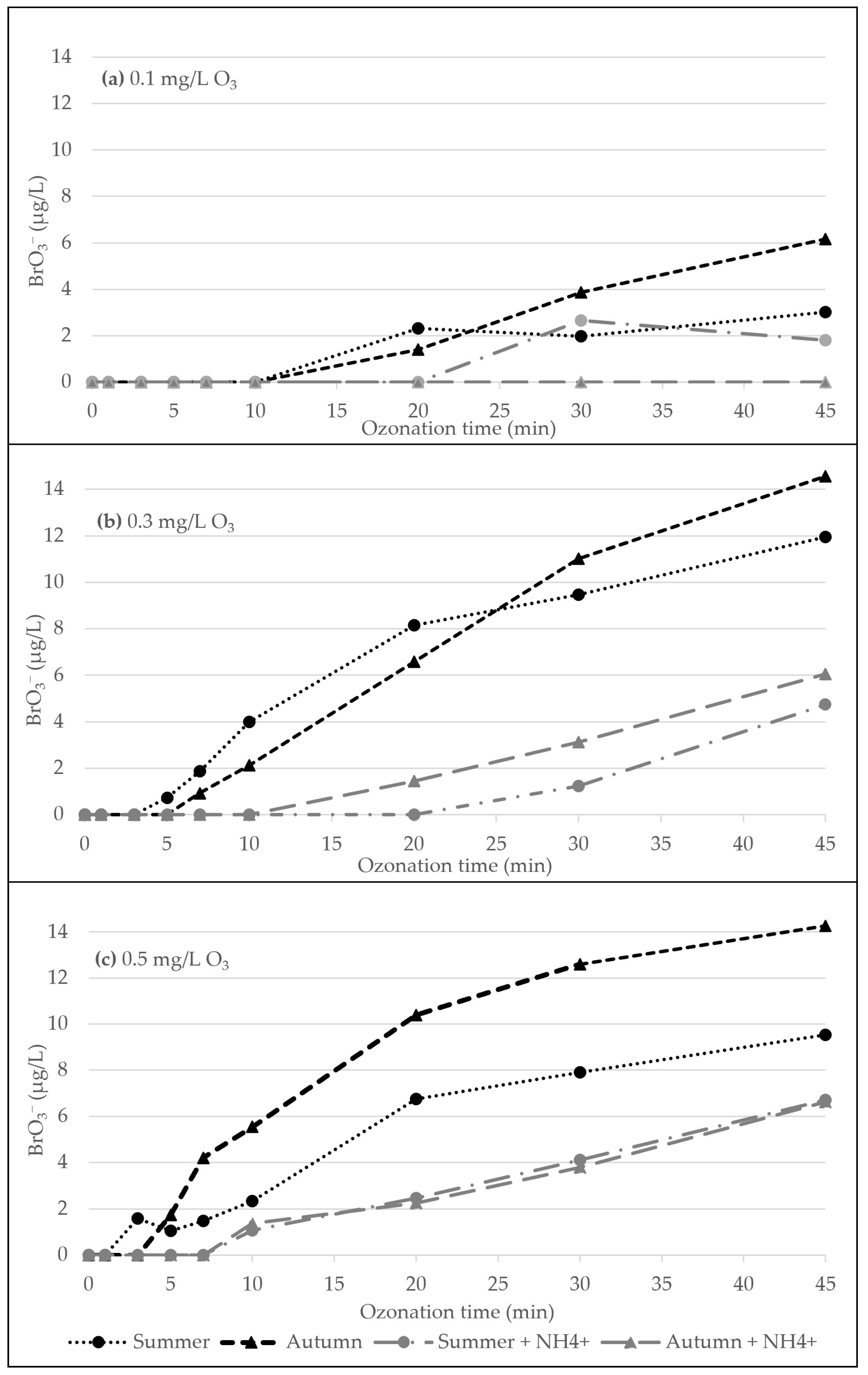
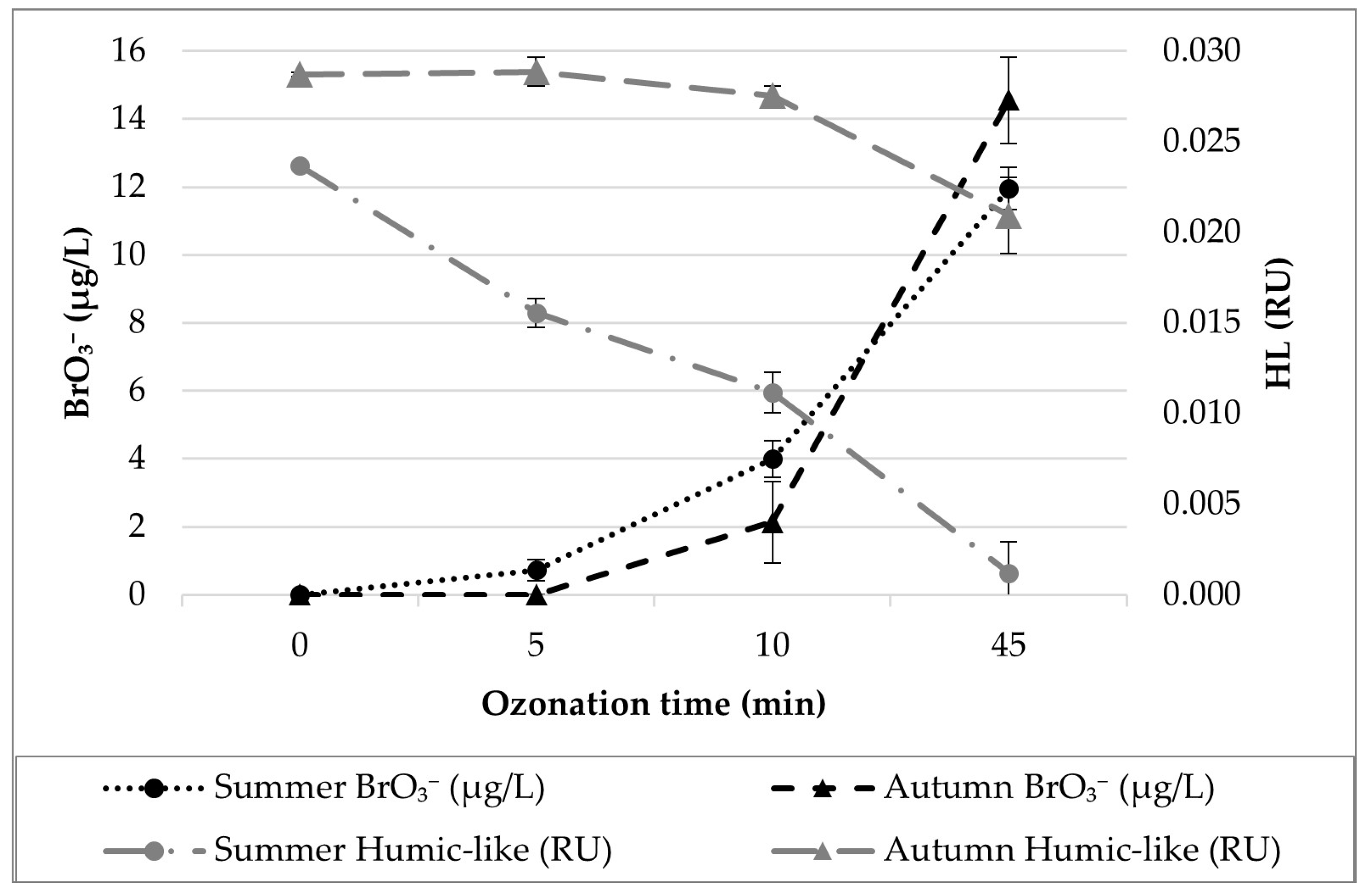
3.1. Ozonation Experiment

The Butoniga water treatment plant is one of the largest producers of drinking water in Croatia that uses ozonation, and in recent years bromate has been detected in the treated water because the raw surface water from the reservoir contains bromides (<20 µg/L), which are the precursors of bromate in the ozonation process. According to the literature, this surface water should have no potential for bromate formation because it contains less than 20 µg/L of bromide [16]. It was necessary to investigate correlations between bromide, bromate, and other water quality parameters with the applied ozone doses to determine their relationship and why this water has this potential for bromate formation.
Two seasons (summer and autumn) were selected to study the effects of raw water quality: when the lake was stratified and when it was not. In the water treatment plant, the main ozonation occurs at lower doses than those used during pre-ozonation but over a much longer period, so this was simulated in the laboratory. The DMRF phase also removes metals such as manganese and iron, which are mainly oxidized by ozone during the pre-treatment, so it was possible to study the effect of ozone in the main ozonation almost exclusively on bromate formation. Although it is known that iron can contribute to the Fenton oxidation process [27], in this work it was assumed that no dissolved metals were present in the samples because they had been previously removed. The organic matter change was observed as UV254, HL, and TL fluorescence instead of total organic carbon or dissolved organic carbon [21,28].
One problem that occurs with raw lake water is temperature stratification in the summer. The lake is relatively shallow (the maximum depth near the dam is 16 m) and there is temperature stratification of water and other water compounds that affect the quality of raw water obtained for drinking water. In the water extraction tower, the water can be taken from four different depths, which allows the selection of water with optimal quality for treatment.
The average raw water results after DMRF are presented in Table 1, with ammonium concentrations found to be below the quantification limit (<0.003 mg/L). Since the mechanism of bromate formation from bromide is very complex, it is difficult to predict the degree of bromate formation without conducting experiments on the specific water to be ozonated [10]. From the water analysis data, it appears that most of the bromate formation occurred only in water after the main ozonation phase, in which the duration was longer, and the ozone dose was higher and remained higher in the next treatment phases. Considering the literature on bromate formation during ozonation, the concentration of residual ozone and ammonium were selected as the variables that could have the greatest influence on bromate formation [29].
Bromate formation (Figure 1a, at the lowest ozone dose of 0.1 mg/L) was observed in the samples without ammonium addition in the 20th minute. In the presence of ammonium, an increase in bromate formation in the summer was observed in the 30th minute, while in the autumn, no bromate was formed after 45 min of ozonation. This could mean that in certain seasons the formation of bromates can be prevented by the addition of ammonium during the treatment with a low dose of ozone. Bromate formation was less than 7 µg/L in all samples, which is below the MCL. Samples treated with an ozone dose of 0.3 mg/L (Figure 1b) showed an increase in bromate levels after 5 min in both seasons, while other samples with added ammonium showed bromate formation after 20 min of ozonation. More bromates were formed in the autumn than in the summer.
At a low residual ozone concentration of 0.1 mg/L (Figure 1a), bromates were detected after 10 min, whereas at ozone concentrations of 0.3 (Figure 1b) and 0.5 mg/L (Figure 1c), formation was visible after 5 min. Although the difference in the amount and rate of bromate formation in water after DMRF was not large at ozone concentrations of 0.3 and 0.5 mg/L, the ozone dose of 0.5 mg/L resulted in faster rates of formation and higher final concentrations. The results suggest that it would be possible to control bromate formation by reducing the ozone dosage and duration. In addition, higher bromate formation was observed in the autumn than in the summer, implying that greater caution should be taken when ozonating water during this time of year.
Von Gunten [16] pointed out that the formation of bromate is the most important problem in ozonation. Furthermore, the effect of organic matter on bromate formation was studied by Song et al. [30], and they concluded that organic matter reduces the formation of bromate. In addition to the effects of organic matter, Siddiqui and Amy [31] and Song et al. [30] found that bromate formation was reduced by increased ammonium concentrations in water. This was also confirmed in this study as the elevated ammonium concentration (0.4 mg/L) in the water reduced the formation of bromate during ozonation for both seasons, and all bromates formed were below the MCL.

3.2. Data Analysis and Modelling

3.2.1. Spearman’s Correlation Matrix

Spearman’s correlation coefficients were calculated to evaluate the correlations between variables in ozonated water. As seen in Table 2, the season was positively correlated with UV254 values, which means that the sample collected in the autumn had significantly higher UV254 values than the sample collected in the summer. UV254 was significantly correlated with water quality as a function of season [32], bromate formation, and ozonation time. Higher HL fluorescence levels were found in the summer period, while higher TL fluorescence levels were found in the autumn period. Since UV254 is associated with organic matter, it can be concluded that samples collected in the autumn have a higher concentration of organic matter. The Br concentration was significantly lower in the samples collected in the autumn so it was expected that fewer bromates would form in the water collected in the summer than in the water collected in the autumn. Bromides showed a negative but significant correlation with season, ozonation time, and bromate formation. The levels of Br, UV254, HL, and TL were dependent on time of year, indicating that water composition varies significantly with sampling time [33].
Ozone dose was positively correlated with BrO3 content, with higher ozone dose resulting in higher BrO3 concentrations detected in the samples, consistent with previous studies [11]. Ozonation time significantly affected the levels of UV254, HL, TL, and Br, with the highest value for BrO3 (r = 0.784). Longer ozone treatment times resulted in an increase in BrO3 and TL levels while decreasing UV254, Br, and HL levels. A negative correlation was found between BrO3 concentrations and NH4+, Br, HL, while the TL values showed a positive correlation with BrO3 concentration.
The fluorescent components (HL and TL) were significantly correlated with Br concentration, ozonation time, and each other. Moreover, an increase in the levels of HL showed a decrease in TL levels, as indicated by a negative Spearman’s correlation coefficient (r = −0.676). HL was significantly correlated with Br, while a decrease in Br was followed by the formation of TL. Bromate formation was significantly correlated with decreases in UV254, Br, and HL values, while bromate was positively correlated with TL formation and increased with dose and duration of ozonation. Li et al. [34] observed appreciable bromate formation only after UV254 and HL fluorescence values in ozonated samples decreased compared to their initial values. In this research, there were negative correlations between bromate and HL fluorescence. R2 coefficients were in the range from −0.76 (samples with ammonium addition) to −0.998 (without ammonium addition). An example of this correlation can be seen in Figure 2 for an ozone dose of 0.3 mg/L which shows the decomposition of HL fluorescence as bromate was formed.
The addition of ammonium decreased the BrO3 content in this study during the ozonation experiment, as previously determined by Siddiqui and Amy [31] and Song et al. [30]. However, according to the Spearman’s rank-order correlation in this study, NH4+ addition had no other significant correlation with the remaining output parameters. This was expected since the addition was performed in a laboratory experiment, whereas these four outputs were associated with raw water quality after DMRF.

3.2.2. Multiple Linear Regression and Piecewise Linear Regression Models

The effects of season (X1), the ozone dose (X2), the ozonation time (X3), and the presence of NH4+ (X4) on UV254, BrO3, Br, HL, and TL fluorescence were analyzed by multiple linear regression, piecewise linear regression, and artificial neural networks. The performance of MLP and PLR models was evaluated based on R2, Radj2, and SEE.
Parameters of the MLR and PLR models were estimated using the Levenberg–Marquardt algorithm implemented in Statistica v14.0. The obtained values, as well as the basic statistical analysis of the developed models, are given in Table 3. The results for the multiple linear regressions (Table 3) show the best agreement between the model-predicted data and experimental data obtained for the Br content (R2adj = 0.8056), followed by UV254 (R2adj = 0.7579). On the other hand, the highest dissipation between the model and experimental data was obtained for the TL values (R2adj = 0.6173). Furthermore, statistical analysis of the MLR models revealed that dose and time of ozonation had a significant positive effect on bromate formation, while the presence of ammonium led to a decrease in bromate formation. Season, time, and ozone dose contributed significantly to the decrease in bromide concentration, while this effect was much smaller in the presence of ammonium. Since bromates are formed from bromides, it is logical that as bromide concentration decreases, bromate concentration increases. Therefore, the factors that affect the reduction of bromide also affect the formation of bromate and vice versa.
According to Ryan and Porth [35], when working with variables that have various linear connections over different ranges, a single regression cannot accurately capture the relationship between model input and model output variables. Therefore, PLR can be used as an efficient alternative. The PLR models explained the experimental data with more precision than the MLR models in this study. Linear regression computes an equation that minimizes the distance between the fitted line and all the data points. A model fits the data well in general if the differences between the observed and predicted values are small. The concept behind piecewise linear regression is that if the data demonstrate distinct linear patterns through various parts of the data, the regression function should be modelled in pieces. In this work, the data regression model was fitted to the data for two ranges of x, x ≤ bn and x > bn; therefore, piecewise linear regression ensured better agreement between the experimental data and model-predicted data. When a multiple linear regression model was utilized, for example, the agreement between the experimental and model-predicted data for BrO3 was quite poor (R2adj = 0.7091). The piecewise linear regression method ensured high agreement between the experimental and model data (R2adj = 0.9494). Furthermore, according to the developed MLR and PLR models, the presence of ammonium and ozone had no significant effect on HL and TL values. Ozonation time and season, which affect water quality and composition, had significant positive effects on TL and a significant negative effect on HL. The value of HL decreased with the change of season and a longer ozonation time, while at the same time the value of TL increased. It can be concluded that part of HL converts to TL components. A similar phenomenon was observed with the decrease in bromide concentrations while the bromate concentrations increased.
The proposed multiple linear regression models as well as the piecewise linear regression models were both found to be statistically significant (for p < 0.05) with p-values < 0.001 (Table 3). Statistical analysis (ANOVA) revealed that the F-values were likewise high (in the range from 28.43 to 118.44), compared to F-critical. Higher F-test values and lower p-values, according to Pilkington, Preston and Gomes [36], show the relative significance of the derived models. The gathered findings demonstrated the validity of the created models throughout the spectrum of variables evaluated.

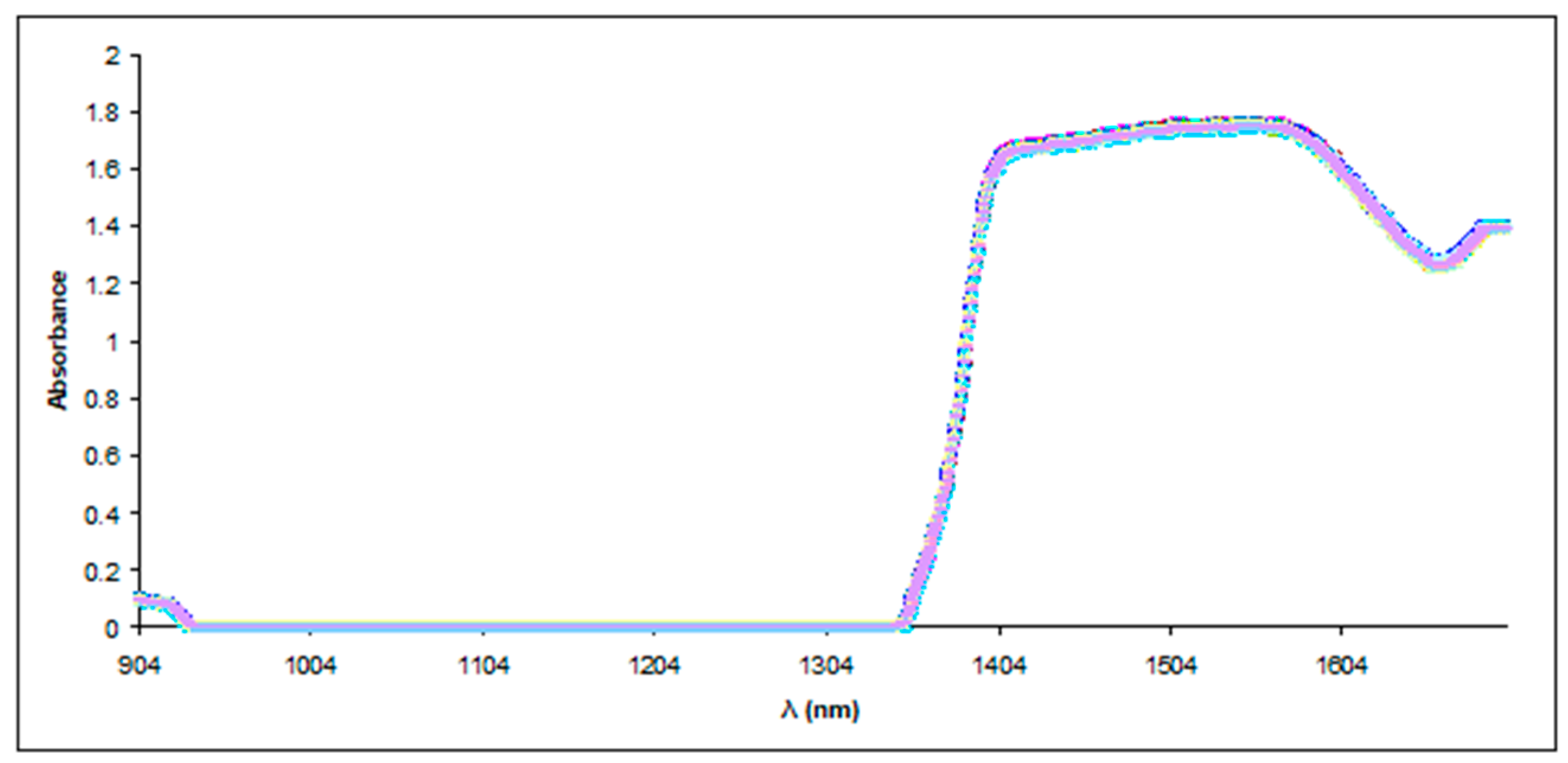
3.2.3. Near-Infrared (NIR) Spectroscopy and Principal Component Analysis (PCA)
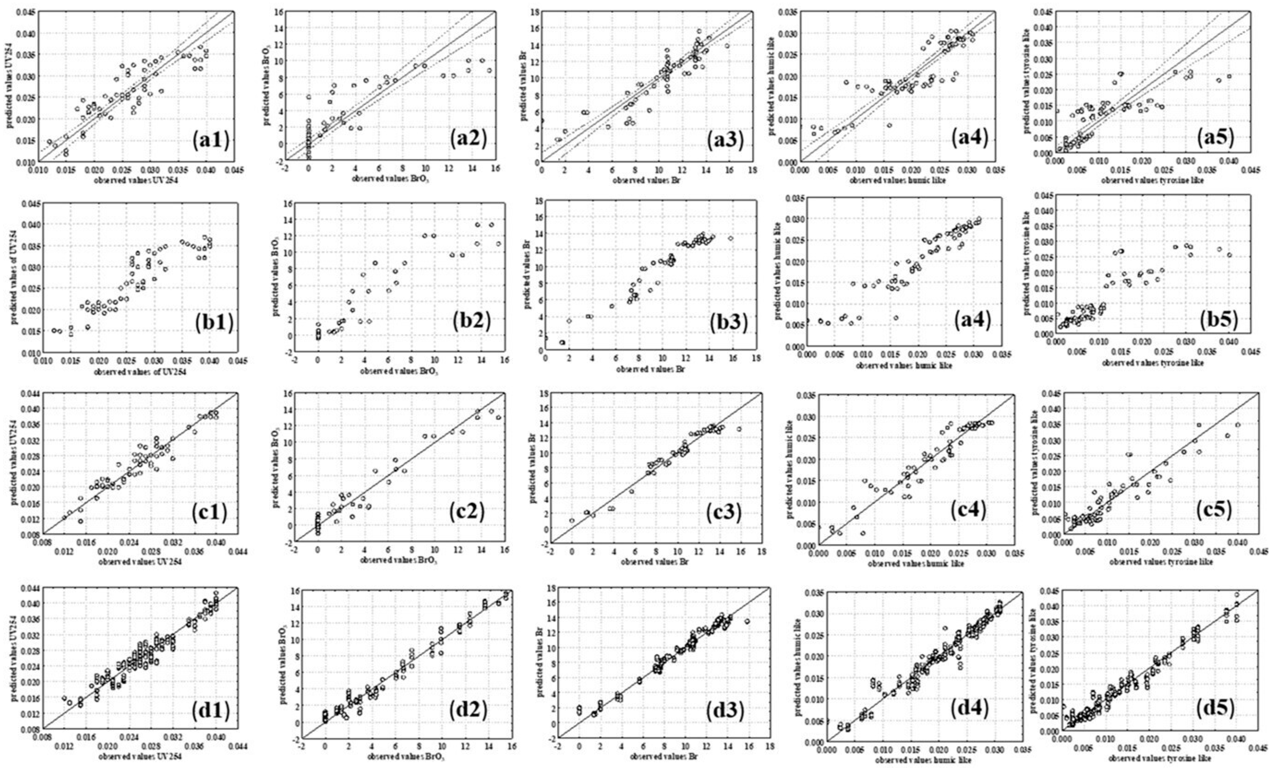
Near-infrared spectroscopy is a specific method where one cannot determine which peak of spectra is correlated to a specific compound without the use of chemometrics. Therefore, in this case principal component analysis was used. The goal of the PCA was to extract data in the form of principal components (factors) that will later be used for artificial neural network modelling. The raw spectra presented in Figure 3 showed slight differences that are sometimes not visible from such a large dataset when presented in this way.
There is also a visible area where spectra overlap (940–1355 nm), which is specific for water samples [37]. For further analysis, via PCA, the spectral range from 1355 to 1699 was used. The initial dataset comprised 36 water samples (each recorded five times) measured two times (July (summer) and September (autumn)), resulting in a datasheet of 360 rows (samples) and 344 columns (number of wavelengths). With the use of PCA, this dataset was decreased to 360 rows (samples) and 10 columns (i.e., the first 10 factors from the PCA). The first 10 factors were selected for further analysis since they represent 99.9% of variability in samples.

3.2.4. ANN Models

To test the applicability of ANN models for describing the ozonation process, two different approaches were used: (i) input for artificial neural networks without NIR spectra; (ii) input for artificial neural networks consisted of input that was used for the first approach with the addition of the PCA-derived data for the NIR spectra (10 additional variables). The selection of the optimal neural network was performed based on the linear coefficient of determination (R2) and on the RMSE between the measured value and the model-predicted value. The ANN models were run by splitting the data into 70:15:15 training, testing, and validation sets, as this gave the best results in terms of not overfitting or underfitting the model out of all the ratios tested (50:30:20, 60:20:20, 70:20:10, 70:15:15). The back error propagation algorithm available in Statistica v14.0 was used for model training.
The characteristics of the selected developed neural networks are given in Table 4. In cases where ANN models were developed using the parameters “season”, “ozone dose”, “ozonation time”, and “presence of NH4+“ for the simultaneous prediction of UV254, BrO3, Br, HL, and TL fluorescence, MLP 4-8-5 was selected as optimal. The selected ANN model included four neurons in the input layer, eight neurons in the hidden layer, and five outputs. Based on the R2 values of training, testing, and validation, this ANN model produced the highest values with the lowest errors. Comparisons between the experimental and model-predicted data are given in Figure 4, while a detailed overview of the selected ANN performance is provided in Table 5. Notably, when using the selected ANNs, the lowest R2 values for validation were obtained for HL (0.9365) and the highest for Br (0.9775), which confirmed the applicability of the ANN modelling for simulation description of several output variables [38,39].
Prior to the use of the NIR spectra as input data for ANNs, a PCA was performed. The first 10 factors derived from the NIR spectra, which explained 99.9% of the variance [20,40,41], were used as input variables along with the first four variables (time and dose of ozonation, ammonium, season) for the ANN development. As in the previous case, the effect of different number of neurons was tested, and in this case the range was 3–14 neurons. In addition, the models of ANNs were run with a 70:15:15 split of the data into training, testing, and validation sets, which again gave the best results in terms of R2 values with the lowest errors. Based on the results presented in Table 4, which lists five of the best-fitting ANNs, MLP 14-14-5 was selected as the best-fitting network in terms of R2 values for training, testing, and validation, which were 0.9916, 0.9826, and 0.9732, respectively, and had the lowest errors. Compared to the MLR and PLR results presented in Table 3 and Figure 4, higher values for training, testing, and validation were obtained for all five analyzed output variables. As in the earlier work of Kim et al. [37] which related to wastewater constituents, ANNs show a promising way to explain nonlinear interactions between process variables used in water treatment.
The model can serve as a guide for waters with different characteristics, but the result is not reliable. Model deviation due to climate change could be expected since the WHO notes that several potential changes in water quality may occur as a result of a global increase in the frequency and magnitude of extremely high temperatures and more frequent and intense heavy precipitation, including impacts on sediment loading, chemical composition, total organic carbon content, and microbial composition [42]. ANN structures were not determined based on the specific rules but on a trial-and-error basis. Although artificial neural networks have been demonstrated to be a useful tool for modelling complicated connections between input and output variables, their use in experimental data fitting may have some drawbacks that have to be taken into consideration when developing an ANN model. The first of them is overfitting. As described previously [43], ANN overfitting is evident when the error on the testing or validation dataset is significantly higher than the error on the training dataset. According to Table 4, overfitting was not evident for the ANN models developed in this work. Furthermore, ANN models can be considered as black-box models in the sense that, while they can estimate any function, examining its structure provides no information about the structure of the function being approximated [44]. Based on that, ANN models can be thought highly sensitive to the quality and quantity of input data [45]. Moreover, when developing the ANN model’s extrapolation capacity, the proposed model must be tested so that model predictively is estimated on an individual set of data [46], and computation complexity has to be taken into consideration [47]. As such, this could be considered as a potential limitation of this study.

4. Conclusions

In this work, the influence of season, ozonation dose and duration, and ammonium addition during ozonation of surface water on the concentration of bromides, bromates, UV254, NIR spectra, and fluorescent components (HL and TL substances) in drinking water was analyzed. The Spearman’s correlation analysis showed that season, ozonation dose, and time had significant correlations with all output variables, especially bromate formation, while ammonium affected only bromate and no other outputs. Moreover, the results showed that the MLR models ensured high R2 coefficients (0.82 for bromides prediction), while the PLR models had even higher R2 (up to 0.98 for bromides), and all input variables had a significant effect on bromides. For both MLR and PLR models, season had no significant effect on bromate formation, while ammonium addition affected only bromides and bromates. In addition, three of four input variables showed significant correlation with UV254 in both models. ANNs combined with NIR spectra showed a promising way to connect input process variables with output (results) for water treatment. MLP 14-14-5 was selected as the most appropriate ANN model. The R2 values for training, testing, and validation were 0.99, 0.98, and 0.97, respectively, and had the lowest errors. Of all the methods used for data analysis, ANN modelling provided the best performance in terms of R2 values for validation of the tested samples.

Author Contributions

Conceptualization, A.J.T., M.M., J.G.K., M.U.B. and J.Ć.; methodology, M.G., L.S. and J.Ć.; validation, A.J.T., D.V., M.B., T.J., L.K., M.M., J.G.K., M.U.B. and J.Ć.; formal analysis, D.V., L.S., L.K. and J.Ć.; investigation, M.G., A.J.T. and L.S.; writing—original draft preparation, M.G., A.J.T., D.V., M.B. and T.J.; writing—review and editing, M.G., M.M., J.G.K., M.U.B. and J.Ć.; visualization, M.G.; supervision, M.U.B. and J.Ć.; funding acquisition, M.U.B. All authors have read and agreed to the published version of the manuscript.

Funding

This work is part of the project “Mitigating the negative impacts of Climate Change on the treatment of surface water Reservoirs in drinking water production by flocculation and Ozone” (KK.05.1.1.02.0003) by the Croatian Institute of Public Health and the partner of project University of Zagreb, Faculty of Food Technology and Biotechnology. The project received funding from the European structural and investment funds. The total value of the Project is HRK 3,573,786.14.

Data Availability Statement

The data presented in this study are openly available [48].

Acknowledgments

The authors would like to thank the Istrian Water Supply for their cooperation and help with the experiments.

Conflicts of Interest

The authors declare no conflict of interest. The funders had no role in the design of this study; in the collection, analyses, or interpretation of data; in the writing of the manuscript; or in the decision to publish the results.

References

  1. UNESCO. Groundwater 1. Making the Invisible Visible. 2022. Available online: https://reliefweb.int/report/world/united-nations-world-water-development-report-2022-groundwater-making-invisible-visible?gclid=EAIaIQobChMI3cC79Lmh_gIVmAcGAB2QVgh1EAAYASAAEgLLIfD_BwE (accessed on 2 May 2022).
  2. Hou, P.; Chang, F.; Duan, L.; Zhang, Y.; Zhang, H. Seasonal Variation and Spatial Heterogeneity of Water Quality Parameters in Lake Chenghai in Southwestern China. Water 2022, 14, 1640. [Google Scholar] [CrossRef]
  3. Liang, L.; Singer, P.C. Factors Influencing the Formation and Relative Distribution of Haloacetic Acids and Trihalomethanes in Drinking Water. Environ. Sci. Technol. 2003, 37, 2920–2928. [Google Scholar] [CrossRef] [PubMed]
  4. Wada, Y.; Flörke, M.; Hanasaki, N.; Eisner, S.; Fischer, G.; Tramberend, S.; Satoh, Y.; van Vliet, M.T.H.; Yillia, P.; Ringler, C.; et al. Modeling global water use for the 21st century: The Water Futures and Solutions (WFaS) initiative and its approaches. Geosci. Model Dev. 2016, 9, 175–222. [Google Scholar] [CrossRef] [Green Version]
  5. Siddiqui, M.S.; Amy, G.L.; Rice, R.G. Bromate ion formation: A critical review. J. Am. Water Work. Assoc. 1995, 87, 58–70. [Google Scholar] [CrossRef]
  6. Tyrovola, K.; Diamadopoulos, E. Bromate formation during ozonation of groundwater in coastal areas in Greece. Desalination 2005, 176, 201–209. [Google Scholar] [CrossRef]
  7. Milosevic, N.; Thomsen, N.; Juhler, R.; Albrechtsen, H.-J.; Bjerg, P. Identification of discharge zones and quantification of contaminant mass discharges into a local stream from a landfill in a heterogeneous geologic setting. J. Hydrol. 2012, 446–447, 13–23. [Google Scholar] [CrossRef]
  8. De Angelo, A.B.; George, M.H.; Kilburn, S.R.; Moore, T.M.; Wolf, D.C. Carcinogenicity of Potassium Bromate Administered in the Drinking Water to Male B6C3F1 Mice and F344/N Rats. Toxicol. Pathol. 1998, 26, 587–594. [Google Scholar] [CrossRef] [Green Version]
  9. WHO. Bromate in Drinking Water: Background Document for Development of WHO Guidelines for Drinking-Water Quality; WHO: Geneva, Switzerland, 2005. [Google Scholar]
  10. Song, R.; Donohoe, C.; Minear, R.; Westerhoff, P.; Ozekin, K.; Amy, G. Empirical modeling of bromate formation during ozonation of bromide-containing waters. Water Res. 1996, 30, 1161–1168. [Google Scholar] [CrossRef]
  11. Gillogly, T. Bromate Formation and Control during Ozonation of Low Bromide Waters; AWWA Research Foundation and American Water Works Association: Denver, CO, USA, 2001. [Google Scholar]
  12. Wang, Y.; Man, T.; Zhang, R.; Yan, X.; Wang, S.; Zhang, M.; Wang, P.; Ren, L.; Yu, J.; Li, C. Effects of organic matter, ammonia, bromide, and hydrogen peroxide on bromate formation during water ozonation. Chemosphere 2021, 285, 131352. [Google Scholar] [CrossRef]
  13. Uyak, V.; Ozdemir, K.; Toroz, I. Multiple linear regression modeling of disinfection by-products formation in Istanbul drinking water reservoirs. Sci. Total. Environ. 2007, 378, 269–280. [Google Scholar] [CrossRef]
  14. Mandel, P. Modelling Ozonation Processes for Disinfection By-Product Control in Potable Water Treatment: From Laboratory to Industrial Units. 2011. Available online: https://tel.archives-ouvertes.fr/tel-00564767 (accessed on 28 May 2020).
  15. Gregov, M.; Jukić, A.; Ćurko, J.; Matošić, M.; Gajšak, F.; Crnek, V.; Ujević Bošnjak, M. Bromide occurrence in Croatian groundwater and application of literature models for bromate formation. Environ. Monit. Assess. 2022, 194, 544. [Google Scholar] [CrossRef] [PubMed]
  16. Von Gunten, U. Ozonation of drinking water: Part II. Disinfection and by-product formation in presence of bromide, iodide or chlorine. Water Res. 2003, 37, 1469–1487. [Google Scholar] [CrossRef]
  17. Jarvis, P.; Parsons, S.A.; Smith, R. Modeling Bromate Formation During Ozonation. Ozone Sci. Eng. 2007, 29, 429–442. [Google Scholar] [CrossRef] [Green Version]
  18. Legube, B.; Parinet, B.; Gelinet, K.; Berne, F.; Croue, J.-P. Modeling of bromate formation by ozonation of surface waters in drinking water treatment. Water Res. 2004, 38, 2185–2195. [Google Scholar] [CrossRef] [PubMed]
  19. Adamowski, J.; Chan, H.F.; Prasher, S.O.; Ozga-Zielinski, B.; Sliusarieva, A. Comparison of multiple linear and nonlinear regression, autoregressive integrated moving average, artificial neural network, and wavelet artificial neural network methods for urban water demand forecasting in Montreal, Canada. Water Resour. Res. 2012, 48, 3–4. [Google Scholar] [CrossRef]
  20. Valinger, D. Development of Near Infrared Spectroscopy Models for Quantitative Prediction of the Content of Bioactive Compounds in Olive Leaves. Chem. Biochem. Eng. Q. 2018, 32, 535–543. [Google Scholar] [CrossRef]
  21. Shi, W.; Zhuang, W.-E.; Hur, J.; Yang, L. Monitoring dissolved organic matter in wastewater and drinking water treatments using spectroscopic analysis and ultra-high resolution mass spectrometry. Water Res. 2021, 188, 116406. [Google Scholar] [CrossRef] [PubMed]
  22. Balbino, S.; Vincek, D.; Trtanj, I.; Egređija, D.; Gajdoš- Kljusurić, J.; Kraljić, K.; Obranović, M.; Škevin, D. Assessment of Pumpkin Seed Oil Adulteration Supported by Multivariate Analysis: Comparison of GC-MS, Colourimetry and NIR Spectroscopy Data. Foods 2022, 11, 835. [Google Scholar] [CrossRef]
  23. Gajdoš Kljusurić, J.; Boban, A.; Mucalo, A.; Budić-Leto, I. Novel Application of NIR Spectroscopy for Non-Destructive Determination of ‘Maraština’ Wine Parameters. Foods 2022, 11, 1172. [Google Scholar] [CrossRef]
  24. Matilainen, A.; Gjessing, E.T.; Lahtinen, T.; Hed, L.; Bhatnagar, A.; Sillanpää, M. An overview of the methods used in the characterisation of natural organic matter (NOM) in relation to drinking water treatment. Chemosphere 2011, 83, 1431–1442. [Google Scholar] [CrossRef]
  25. Bicanic, D.; Streza, M.; Dóka, O.; Valinger, D.; Luterotti, S.; Ajtony, Z.S.; Kurtanjek, Z.; Dadarlat, D. Non-destructive Measurement of Total Carotenoid Content in Processed Tomato Products: Infrared Lock-In Thermography, Near-Infrared Spectroscopy/Chemometrics, and Condensed Phase Laser-Based Photoacoustics—Pilot Study. Int. J. Thermophys. 2015, 36, 2380–2388. [Google Scholar] [CrossRef]
  26. Brereton, R.G. Graphical introduction to principal components analysis. J. Chemom. 2022, 36, e3404. [Google Scholar] [CrossRef]
  27. Xu, M.; Wu, C.; Zhou, Y. Advancements in the Fenton Process for Wastewater Treatment. In Advanced Oxidation Processes; IntechOpen Limited: London, UK, 2020; pp. 61–77. [Google Scholar] [CrossRef]
  28. Wang, X.; Tong, Y.; Chang, Q.; Lu, J.; Ma, T.; Zhou, F.; Li, J. Source identification and characteristics of dissolved organic matter and disinfection by-product formation potential using EEM-PARAFAC in the Manas River, China. RSC Adv. 2021, 11, 28476–28487. [Google Scholar] [CrossRef]
  29. Buffle, M.-O.; Galli, S.; von Gunten, U. Enhanced Bromate Control during Ozonation: The Chlorine-Ammonia Process. Environ. Sci. Technol. 2004, 38, 5187–5195. [Google Scholar] [CrossRef]
  30. Song, R.; Westerhoff, P.; Minear, R.; Amy, G. Bromate minimization during ozonation. J. Am. Water Work. Assoc. 1997, 89, 69–78. [Google Scholar] [CrossRef]
  31. Siddiqui, M.S.; Amy, G.L. Factors Affecting DBP Formation During Ozone-Bromide Reactions. J. Am. Water Work. Assoc. 1993, 85, 63–72. [Google Scholar] [CrossRef]
  32. Aitkenhead-Peterson, J.A.; McDowell, W.H.; Neff, J.C. Sources, Production, and Regulation of Allochthonous Dissolved Organic Matter Inputs to Surface Waters. In Aquatic Ecosystems; Elsevier: San Diego, CA, USA, 2003; pp. 25–70. [Google Scholar] [CrossRef]
  33. Elovitz, M.S.; von Gunten, U.; Kaiser, H.-P. Hydroxyl Radical/Ozone Ratios During Ozonation Processes. II. The Effect of Temperature, pH, Alkalinity, and DOM Properties. Ozone Sci. Eng. 2000, 22, 123–150. [Google Scholar] [CrossRef]
  34. Li, W.-T.; Cao, M.-J.; Young, T.; Ruffino, B.; Dodd, M.; Li, A.-M.; Korshin, G. Application of UV absorbance and fluorescence indicators to assess the formation of biodegradable dissolved organic carbon and bromate during ozonation. Water Res. 2017, 111, 154–162. [Google Scholar] [CrossRef] [PubMed] [Green Version]
  35. Ryan, S.E.; Porth, L.S. A Tutorial on the Piecewise Regression Approach Applied to Bedload Transport Data. 2007. Available online: https://www.fs.usda.gov/rm/pubs/rmrs_gtr189.pdf (accessed on 13 July 2022).
  36. Pilkington, J.L.; Preston, C.; Gomes, R.L. Comparison of response surface methodology (RSM) and artificial neural networks (ANN) towards efficient extraction of artemisinin from Artemisia annua. Ind. Crops. Prod. 2014, 58, 15–24. [Google Scholar] [CrossRef]
  37. Kim, S.Y.; Ćurko, J.; Gajdoš Kljusurić, J.; Matošić, M.; Crnek, V.; López-Vázquez, C.M.; Garcia, H.A.; Brdjanović, D.; Valinger, D. Use of near-infrared spectroscopy on predicting wastewater constituents to facilitate the operation of a membrane bioreactor. Chemosphere 2021, 272, 129899. [Google Scholar] [CrossRef]
  38. Liu, F.; He, Y.; Wang, L.; Sun, G. Detection of Organic Acids and pH of Fruit Vinegars Using Near-Infrared Spectroscopy and Multivariate Calibration. Food Bioprocess Technol. 2011, 4, 1331–1340. [Google Scholar] [CrossRef]
  39. Urbano-Cuadrado, M.; Luque de Castro, M.D.; Pérez-Juan, P.M.; García-Olmo, J.; Gómez-Nieto, M.A. Near infrared reflectance spectroscopy and multivariate analysis in enology: Determination or screening of fifteen parameters in different types of wines. Anal. Chim. Acta 2004, 527, 81–88. [Google Scholar] [CrossRef]
  40. Jurinjak Tušek, A.; Benković, M.; Malešić, E.; Marić, L.; Jurina, T.; Gajdoš Kljusurić, J.; Valinger, D. Rapid quantification of dissolved solids and bioactives in dried root vegetable extracts using near infrared spectroscopy. Spectrochim. Acta Part A Mol. Biomol. Spectrosc. 2021, 261, 120074. [Google Scholar] [CrossRef]
  41. Valinger, D.; Jurina, T.; Šain, A.; Matešić, N.; Panić, M.; Benković, M.; Gajdoš Kljusurić, J.; Jurinjak Tušek, A. Development of ANN models based on combined UV-vis-NIR spectra for rapid quantification of physical and chemical properties of industrial hemp extracts. Phytochem. Anal. 2021, 32, 326–338. [Google Scholar] [CrossRef]
  42. WHO, Climate-Resilient Water Safety Plans: Managing Health Risks Associated with Climate Variability and Change. 2017. Available online: http://apps.who.int/iris/bitstream/handle/10665/258722/9789241512794-eng.pdf?sequence=1 (accessed on 11 May 2022).
  43. Razavi, S. Deep learning, explained: Fundamentals, explainability, and bridgeability to process-based modelling. Environ. Model. Softw. 2021, 144, 105159. [Google Scholar] [CrossRef]
  44. Bakas, I.; Kontoleon, K.J. Performance Evaluation of Artificial Neural Networks (ANN) Predicting Heat Transfer through Masonry Walls Exposed to Fire. Appl. Sci. 2021, 11, 11435. [Google Scholar] [CrossRef]
  45. Lee, J.H.; Lee, J.Y.; Lee, M.H.; Lee, M.Y.; Kim, Y.W.; Hyung, J.S.; Kim, K.B.; Cha, Y.K.; Koo, J.Y. Development of a short-term water quality prediction model for urban rivers using real-time water quality data. Water Supply 2022, 22, 4082–4097. [Google Scholar] [CrossRef]
  46. El-Sari, B.; Biegler, M.; Rethmeier, M. Investigation of the Extrapolation Capability of an Artificial Neural Network Algorithm in Combination with Process Signals in Resistance Spot Welding of Advanced High-Strength Steels. Metals 2021, 11, 1874. [Google Scholar] [CrossRef]
  47. Kyono, T.; Otsuka, Y.; Fukumoto, Y.; Owaki, S.; Nakamura, M. Computational-Complexity Comparison of Artificial Neural Network and Volterra Series Transfer Function for Optical Nonlinearity Compensation with Time- and Frequency-Domain Dispersion Equalization. In Proceedings of the 2018 European Conference on Optical Communication (ECOC), Rome, Italy, 23–27 September 2018; pp. 1–3. [Google Scholar] [CrossRef]
  48. Gregov, M.; Jurinjak Tušek, A.; Valinger, D.; Benković, M.; Jurina, T.; Surać, L.; Kurajica, L.; Matošić, M.; Gajdoš Kljusurić, J.; Ujević Bošnjak, M.; et al. Data for paper Linear and Non-linear Modelling of Bromate Formation During Ozonation of Surface Water in Drinking Water Production. Zenodo 2023. [Google Scholar] [CrossRef]
Figure 1. Formation of bromate both with and without NH4+ addition at the ozone dosages of (a) 0.1 mg/L, (b) 0.3 mg/L, and (c) 0.5 mg/L.
Water 15 01516 g001
Figure 2. Formation of bromate and decomposition of HL fluorescence at the ozone dose of 0.3 mg/L without NH4+ addition.
Water 15 01516 g002
Figure 3. Raw NIR spectra of all water samples collected in July.
Water 15 01516 g003
Figure 4. Comparison between experimental data and (a) MLR model prediction; (b) PLR model; (c) ANN models without NIR spectra and (d) ANN models with NIR spectra (1) UV254; (2) BrO3; (3) Br; (4) HL; and (5) TL.
Water 15 01516 g004
Table 1. The quality results of raw water after DMRF (average values with standard deviation).
SeasonUV254 (cm−1)BrO3 (µg/L)Br (µg/L)Humic-Like (RU)Tyrosine-Like (RU)
Summer0.039 ± 0.001010.77 ± 0.080.0237 ± 0.00300.0084 ± 0.0026
Autumn0.027 ± 0.002013.20 ± 0.140.0287 ± 0.00240.0026 ± 0.0009
Table 2. The Spearman’s rank-order correlations for all analyzed properties. Values marked bold with * are significant at p < 0.05.
ParameterSeasonOzone Dose (mg/L)Ozonation Time (min)NH4+
(mg/L)
UV254 (cm−1)BrO3
(µg/L)
Br (µg/L)HL (RU)TL (RU)
Season-0.036−0.0060.0110.603*0.021−0.518 *−0.654 *0.672 *
Ozone dose (mg/L)0.036-0.033−0.038−0.2130.265*−0.203−0.0020.075
Ozonation time (min)−0.0060.033-−0.024−0.650*0.784 *−0.650 *−0.583 *0.523 *
NH4+ (mg/L)0.011−0.038−0.024-0.113−0.254 *0.158−0.118−0.183
UV254 (cm−1)0.603 *−0.213−0.650 *0.113-−0.586 *0.185−0.0020.026
BrO3 (µg/L)0.0210.265 *0.784 *−0.254 *−0.586*-−0.760 *−0.498 *0.499 *
Br (µg/L)−0.518 *−0.203−0.650 *0.1580.185−0.760 *-0.766 *−0.770 *
HL (RU)−0.654 *−0.002−0.583 *−0.118−0.002−0.498 *0.766 *-−0.676 *
TL (RU)0.672 *0.0750.523 *−0.1830.0260.499 *−0.770 *−0.676 *-
Table 3. MLR and PLR model coefficients. Values marked bold are significant at p < 0.001. (R2adj = R2 adjusted; SEE = standard error; F-value critical for this dataset was 2.53).
Model Outputb0b1 (Season)b2 (Ozone Dose)b3 (Ozonation Time)b4 (NH4+)Break PointR2R2adjSEEF-Value
MLRUV2540.019 ± 0.0020.009 ± 0.001−0.010 ± 0.003−2.430 × 10⁻⁴ ± 2.500 × 10−50.002 ± 0.002 0.77220.75790.003654.227
BrO3−0.529 ± 1.033−0.610 ± 0.5465.961 ± 1.7090.181 ± 0.015−4.976 ± 1.4320.72620.70912.264242.434
Br16.840 ± 0.739−2.284 ± 0.390−4.896 ± 1.222−0.160 ± 0.0113.808 ± 1.0250.81700.80561.619671.442
HL0.040 ± 0.002−0.009 ± 0.001−0.002 ± 0.003−2.670 × 10⁻³ ± 2.500 × 10⁻⁴−0.003 ± 0.0020.78570.77230.003758.668
TL−0.009 ± 0.0030.011 ± 0.0010.003 ± 0.0042.630 × 10−3 ± 3.800 × 10⁻⁵−0.005 ± 0.0040.63980.61730.005628.429
PLRUV2540.019 ± 0.001
0.025 ± 0.011
0.005 ± 0.001
0.006 ± 0.002
−0.004 ± 0.001
−0.011 ± 0.004
−1.680 × 10⁻⁴ ± 1.248 × 10⁻⁵
−2.180 × 10⁻⁴ ± 1.113 × 10⁻⁵
3.160 × 10⁻⁴ ± 1.111 × 10⁻⁵
0.001 ± 0.001
0.0260.91870.91361.7277 × 10−5118.437
BrO3−0.492 ± 0.025
−1.437 ± 0.078
0.186 ± 0.044
−1.370 ± 0.069
1.037 ± 0.128
11.681 ± 0.887
0.038 ± 0.012
0.226 ± 0.056
−0.589 ± 0.023
−14.181 ± 0.785
2.4660.95240.94943.5157 × 10−5110.241
Br16.519 ± 0.987
16.229 ± 0.547
−0.526 ± 0.011
−2.604 ± 0.147
−13.039 ± 0.567
−0.906 ± 0.025
−0.180 ± 0.004
−0.065 ± 0.007
10.907 ± 0.147
0.960 ± 0.221
10.0090.97530.97371.2528 × 10−5105.138
HL0.043 ± 0.001
0.031 ± 0.003
−0.013 ± 0.004
−0.004 ± 0.001
−0.003 ± 0.001
0.005 ± 0.001
−2.340 × 10⁻⁴ ± 1.870 × 10⁻⁵
−1.530 × 10⁻⁴ ± 3.125 × 10⁻⁵
0.001 ± 0.001
−0.005 ± 0.002
0.0200.95070.94762.1110 × 10−6110.641
TL6.250 × 10−4 ± 2.011 × 10⁻⁵
−0.007 ± 0.001
0.004 ± 0.002
0.011 ± 0.007
−0.002 ± 0.001
0.006 ± 0.003
8.900 × 10⁻⁵ ± 2.155 × 10⁻⁶
2.260 × 10⁻⁴ ± 1.118 × 10⁻⁵
−0.004 ± 0.001
0.001 ± 0.001
0.0110.89230.88551.1199 × 10−775.402
Table 4. Characteristics of the generated artificial neural networks.
ANN StructureTraining perf./
Training Error
Test perf./
Test Error
Validation perf./
Validation Error
Hidden ActivationOutput Activation
ANN models without NIR data as the model inputMLP 4-5-50.9401
0.0179
0.9386
0.0191
0.9328
0.0175
TanhIdentity
MLP 4-9-50.9646
0.0106
0.9630
0.0113
0.9530
0.0124
TanhTanh
MLP 4-6-50.9447
0.0176
0.9445
0.0179
0.9318
0.0184
ExponentialExponential
MLP 4-8-50.9685
0.0097
0.9681
0.0099
0.9581
0.0110
ExponentialLogistic
MLP 4-6-50.9321
0.0194
0.9225
0.0221
0.9185
0.0164
LogisticTanh
ANN models including NIR data as the model inputMLP 14-14-50.9899
0.0031
0.9811
0.0062
0.9717
0.0071
LogisticTanh
MLP 14-14-50.9916
0.0025
0.9826
0.0059
0.9732
0.0067
TanhLogistic
MLP 14-13-50.9814
0.0057
0.9726
0.0097
0.9616
0.0114
ExponentialExponential
MLP 14-8-50.9838
0.0050
0.9789
0.0070
0.9737
0.0068
LogisticExponential
MLP 14-11-50.9878
0.0037
0.9806
0.0064
0.9755
0.0065
LogisticLogistic
MLP 14-14-50.9899
0.0032
0.9811
0.0063
0.9717
0.0071
LogisticTanh
Table 5. Coefficients of determination of analyzed output variables based on selected ANNs.
Model OutputTrainingTestValidation
ANN models without NIR data as the model inputUV2540.97120.96200.9431
BrO30.97600.98110.9623
Br0.98240.99030.9774
HL0.96220.97130.9365
TL0.93110.91040.9459
ANN models including NIR data as the model inputUV2540.97890.96570.9559
BrO30.98980.99210.9876
Br0.98510.99160.9795
HL0.98480.97350.9688
TL0.98030.97160.9766
Disclaimer/Publisher’s Note: The statements, opinions and data contained in all publications are solely those of the individual author(s) and contributor(s) and not of MDPI and/or the editor(s). MDPI and/or the editor(s) disclaim responsibility for any injury to people or property resulting from any ideas, methods, instructions or products referred to in the content.

