Comparing Single and Multiple Imputation Approaches for Missing Values in Univariate and Multivariate Water Level Data

Abstract

Missing values in water level data is a persistent problem in data modelling and especially common in developing countries. Data imputation has received considerable research attention, to raise the quality of data in the study of extreme events such as flooding and droughts. This article evaluates single and multiple imputation methods used on monthly univariate and multivariate water level data from four water stations on the rivers Benue and Niger in Nigeria. The missing completely at random, missing at random and missing not at random data mechanisms were each considered. The best imputation method is identified using two error metrics: root mean square error and mean absolute percentage error. For the univariate case, the seasonal decomposition method is best for imputing missing values at various missingness levels for all three missing mechanisms, followed by Kalman smoothing, while random imputation is much poorer. For instance, for 5% missing data for the Kainji water station, missing completely at random, the Kalman smoothing, random and seasonal decomposition methods had average root mean square errors of 13.61, 102.60 and 10.46, respectively. For the multivariate case, missForest is best, closely followed by k nearest neighbour for the missing completely at random and missing at random mechanisms, and k nearest neighbour is best, followed by missForest, for the missing not at random mechanism. The random forest and predictive mean matching methods perform poorly in terms of the two metrics considered. For example, for 10% missing data missing completely at random for the Ibi water station, the average root mean square errors for random forest, k nearest neighbour, missForest and predictive mean matching were 22.51, 17.17, 14.60 and 25.98, respectively. The results indicate that the seasonal decomposition method, and missForest or k nearest neighbour methods, can impute univariate and multivariate water level missing data, respectively, with higher accuracy than the other methods considered.

1. Introduction

Water level is a measure of water depth in rivers/basin/lakes within a given place over time. Studying water level is important as it can provide warnings for flood risk, which helps to limit the impact of flood disasters on the local population and is also crucial for effective water resources management and for policy makers [1]. The study of water level is also important for the health of a river, to determine the required level for plants and animals to survive at various times of year [2].

Khalifeloo [3] states that recent extreme events globally, such as flooding, drought and bush burning, among other natural disasters, were caused largely by climate change, and these have attracted the attention of researchers to try to provide solutions. Accurate prediction of such extreme events can allow mitigating measures to be implemented. However, much water level/hydrological data is complicated by missing observations, especially in developing countries [4,5], which makes accurate prediction very difficult.

This data gap is a persistent and common problem faced by researchers in data modelling [6,7] and the impact of missing data in modelling depends partly on the proportion of missing data [8]. Imputation studies to minimise missing data in hydrological-related areas have received considerable attention [9]. Various imputation methods providing promising solutions, including regression-based imputation, expectation-maximisation, and multiple imputations (MI), have been introduced to handle missing data [10]. However, selecting a particular imputation approach depends on the process generating the original data; for instance, hydrological data very often exhibit variability due to spatial and temporal phenomena [11,12]. Imputation methods based on statistical models can account for such behaviours and may be used to fill in missing data in hydrological data such as precipitation, streamflow and water level data.

Missingness in water level data, especially for developing countries, can arise for various reasons, including electrical power outage or digital sensor issues, bad weather, faulty data entry from operators, faulty instruments, security challenges and network coverage [13,14,15,16]. Ignoring missing values in a dataset will amount to loss of information and efficiency, and unreliable results, especially where there is a large proportion of missing data [6]. Further effects of incomplete data include complications in data handling, computation and data analyses [17]. Finally, results of statistical analyses may be biased, causing misleading conclusions [18,19].

Various approaches to missing data problems have been used, prominent among which are data deletion (complete-case analysis or available-case analysis) and single imputation [20]. The former approach is criticised because it reduces sample size and can make statistical analysis difficult, especially for temporal data [7]. It also ignores the causes of missingness [8]. However, the latter approach maintains the original sample size and provides a basis for smooth statistical analyses [21].

Single imputation involves replacing each missing value with a single value [22], whereas the alternative, MI, generates two or more values for each missing value [23]. A few single imputation methods are mean, median, mode and random imputations. Despite their usability, most single imputation methods underestimate variance or uncertainty about the missing values, which yields invalid tests and confidence intervals since the estimated values are derived from the ones present, and may also produce biased parameter estimates [10,24,25]. They also ignore relationships between variables [26]. Therefore, MI is preferred where applicable. The availability of these advanced methods in software (especially MI) enables researchers to readily replace missing values with imputed values [27].

The MI method was first proposed by Rubin [28] and simply replaces each missing value by a vector of $D$ imputed values, $D\ge 2$. The $D$ values are ordered in the sense that $D$ completed datasets can be created from the imputed vectors; replacing each missing value with the first component in its vector of imputations creates the first completed dataset; replacing each missing value with the second component in its vector creates the second completed dataset, and so on [29]. In another definition [25], MI is said to be the act of replacing the nonresponse item in the dataset with more than one value; as a result of which, several datasets will be created from it. It has been argued that no single set of imputations or methods of imputation can satisfy all missing data [6], which implies that one method may be better than another method for a particular type of data.

Some more sophisticated single imputation methods for handling univariate time series, comprising the seasonal decomposition, random and Kalman smoothing methods, are available in the imputeTS package in the R software [30]. The authors recommended Kalman smoothing and the seasonal decomposition methods for imputing complex univariate time series data. Wijesekara and Liyanage [31] found Kalman smoothing to be the best method for imputing air quality data. Kalman smoothing is robust for smaller datasets and recommended for imputing high-resolution data [32,33,34]. The seasonal decomposition method was identified as the most effective for imputing univariate time series by Moritz et al. [35].

Other studies include Jadhav et al. [36], who compared imputation methods on five numeric datasets and based on the root mean square error (RMSE) statistic found that k nearest neighbour (kNN) imputation outperformed another six methods comprising mean, median, predictive mean matching (PMM), Bayesian linear regression, linear regression (non-Bayesian) and random methods. Alsaber et al. [37,38] identified missForest and kNN as appropriate to impute both continuous and categorical variables, compared to Bayesian principal component analysis, expectation maximisation with bootstrapping, PMM, kNN and random forest methods for imputing rheumatoid arthritis and air quality datasets, respectively, using RMSE and mean absolute error criteria.

In the last decade, the application of imputation techniques for missing data in hydrological studies has received increasing interest. Ben Aissia et al. [39] recommend multiple imputation rather than mean or interpolation imputation methods for multivariate missing data in hydrological frequency analysis. Various imputation methods which can be used for hydrological missing data, including the arithmetic mean, median and regression-based methods, and imputation based on principal components and multiple imputation were reviewed in Gao et al. [10], who recommended the use of autoregressive conditional heteroscedasticity models for imputation, since these can produce accurate forecasts of non-constant volatility and incorporate heteroscedasticity, which are synonymous with hydrological data. Hamzah et al. [40] evaluated three methods for estimating missing values of daily streamflow from the Langat River basin, namely robust random regression imputation, kNN and classification and regression trees (CART); each of these methods was combined with multiple linear regression (MLR), and based on RMSE and mean absolute percentage error (MAPE) statistics, CART-MLR was said to be the best imputation method. A similar follow-up study found hybridised CART-MLR to be best for all considered missing data percentages, followed by PMM-MLR based on Adj R², root square error and MAPE statistics [41].

To the best of our knowledge, these various approaches to imputation have not been fully exploited in imputing missing values for hydrological data such as water level discharge in Nigeria. However, the work in [13] for the first time introduced the concept of MI for imputing annual peak river discharge, which is vital for flood frequency estimation. The authors compared satellite radar altimetry and MI for five hydrological stations, namely Baro, Lokoja, Umaisha, Onitsha and Taoussa stations. It was concluded that for a dataset with 3 years or fewer missing values, both methods can be utilised. However, for data with more than 3 years missing, radar altimetry was better. Oyerinde et al. [42] used the PMM method to impute missing data from 22 water discharge stations with different missing percentages from 2–70% and recommended PMM for imputing data gaps in data from the Niger basin. However, these two studies failed to consider the missing data mechanism/pattern, which is important for imputing missing data. In addition, they failed to consider single imputation methods, which are frequently suitable for imputing complex univariate time series [30].

This paper presents a comparative study of single and multiple imputation methods for missing values in water level discharge time series data from four water stations on the major rivers Benue and Niger in Nigeria, assuming three missing data mechanisms in each case. The three single imputation methods used are Kalman smoothing and the random and seasonal decomposition methods for the Kainji water station on the river Niger. Four imputation methods comprising random forests, missForest, kNN and PMM were used to impute missing data from the Ibi, Makurdi and Umaisha water stations on the river Benue. The results should be helpful for selecting a suitable imputation approach in future water level studies where data are missing and the probable missing data mechanism can be identified.

A number of key abbreviations are used in this paper and these are summarised in Abbreviations, for reference.

2. Materials and Methods

This section will briefly describe the study area and the methodology for the analysis.

2.1. Study Area

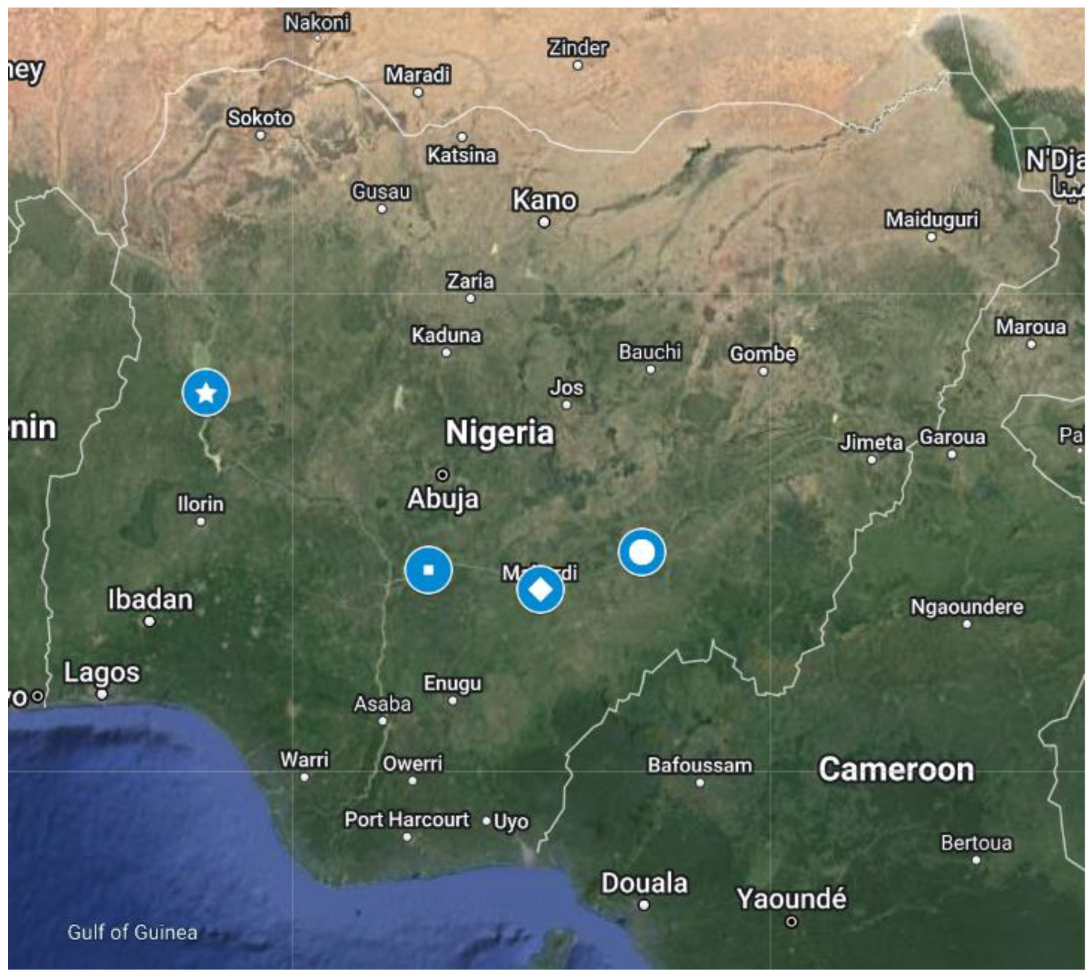
The Kainji water station on river Niger, and Ibi, Makurdi and Umaisha water stations on the river Benue (

Table 1. Characteristics of the selected water stations.

Water Station	State	River	Established (Year)	Time (Month)	Latitude (Degrees)	Longitude (Degrees)
Kainji	Niger	Niger	1980	2010–2016	10.0300	4.6000
Ibi	Taraba	Benue	1980	2011–2016	8.1800	9.7200
Makurdi	Benue	Benue	2010	2011–2016	7.7500	8.5300
Umaisha	Nasarawa	Benue	1980	2011–2016	7.9800	7.2000

Note: Source: NIHSA.

, Figure 1) were chosen as the study area. The two rivers cut across various states in the northern part of Nigeria, with confluence at Lokoja in Kogi state. There are 194 water monitoring stations currently in the country, mostly located along the rivers and dams, to monitor the movements of water level discharges. From these 194 stations available, four water stations were selected as having more up-to-date data than the rest, as some stations have no records from 1980 to date and some have 2 years of records only, for example, as found from a summary of the Nigeria Hydrological Services Agency (NIHSA) records. The main reasons for the data gaps at these water stations are that some people in most communities close to the stations vandalised instruments and/or there were faulty recording instruments.

The dataset from Kainji water station obtained from NIHSA is complete; hence, it was used for the univariate imputation directly. However, Ibi, Makurdi and Umaisha stations have 28, 49 and 23 missing observations in the monthly water levels, respectively, or 39%, 68% and 32% missing data percentages, and the predictive mean matching (PMM) imputation method was used first to impute these missing values for the purposes of this study. To avoid influence of this choice on the results of this study, time series models were fitted to these completed data and the datasets used for the multivariate imputation were simulated from these fitted models. The seasonal autoregressive integrated moving average models (4,0,1)(1,0,1); (2,0,2)(1,0,1); and (1,0,2)(1,0,1) were found to be the best fitting models for Ibi, Makurdi and Umaisha stations, respectively.

Since the Ibi, Makurdi and Umaisha water stations are all located on the river Benue and the observations are recorded at the same time-points for all three stations, we combined these water level datasets to generate multivariate data, representing water levels at three locations on the river, and data deletion and imputation were conducted on these combined data. After imputation, the simulated (complete) data and the imputed data were compared for each water station separately to obtain the two performance metrics.

2.2. Missing Data Mechanisms

Before imputing data, it is important to know the reason why the data are missing. The three missing data mechanisms under which missingness occurs comprise missing completely at random (MCAR), missing at random (MAR), and missing not at random (MNAR) [43], reviewed briefly below.

2.2.1. Missing Completely at Random

A data value is said to be MCAR if the probability of missingness is the same for all units in the sample. This implies that the cause of missingness in the data is independent of the data itself. Following Santos et al. [44], suppose $X$ is a data matrix of order $n\times p$ and $x_{i,j}$ represents the (i,j)th element in $X,$ where $i=\mathrm{1,2},\cdots ,n$ represents the cases and $j=\mathrm{1,2},\cdots ,p$ represents the variables in the sample. Let $X$ be divided into $X_{obs}$ and $X_{mis}$ representing the observed and missing values, respectively, and suppose we also have an indicator matrix $R$ of order $n\times p,$ which indicates whether the element $x_{i,j}$ is missing or not: if $r_{i,j}=0$, then $x_{i,j}$ is missing, otherwise $r_{i,j}=1$ implies $x_{i,j}$ is observed. Then the probability distribution for MCAR can be written as in Equation (1):

$$P\left(R=0|X,\omega \right)=P\left(R=0|\omega \right),$$

(1)

where $\omega$ is the parameters of the missing data in the model.

2.2.2. Missing at Random

Under the MAR mechanism, the probability of missingness may depend on the observed data but not on the value(s) missing, as in Equation (2):

$$P\left(R=0|X,\omega \right)=P\left(R=0|X_{obs},\omega \right).$$

(2)

2.2.3. Missing Not at Random

The MNAR mechanism is present when the probability of missingness in a variable is said to be dependent on the observed and unknown data, which implies that the missing data may be associated with both $X_{obs}$ and $X_{mis}$, as in Equation (3):

$$P\left(R=0|X,\omega \right)=P\left(R=0|X_{obs},X_{mis},\omega \right).$$

(3)

2.3. Imputation Methods for Univariate and Multivariate Data

Imputation methods used here for univariate and multivariate data are briefly described below.

2.3.1. Imputation Methods for Univariate Water Level Time Series Data

Three single imputation methods are used, namely Kalman smoothing and the seasonal decomposition and random methods. These methods, especially Kalman smoothing and seasonal decomposition, were selected to impute univariate water level because they frequently produce best results for longer and complex time series data [30].

All three of these methods were implemented here using the R package imputeTS version 3.3, for univariate time series imputation.

Kalman Smoothing Method

The Kalman smoothing method operates on a basic structural model or the state space representation of an autoregressive integrated moving average (ARIMA) model [30]. The origin of Kalman smoothing may be traced back to R.E. Kalman, who introduced a recursive solution to the discrete-data linear filtering problem in 1960, and over time the method has received much interest, particularly in autonomous and assisted navigation [45]. A Kalman filter, as defined by Maybeck [46], is an optimal recursive data processing algorithm which utilises all available information, irrespective of precision, to estimate the variable of interest. Welch and Bishop [45] defined the Kalman filter and smoother as a set of mathematical equations which efficiently compute the posterior distribution over latent states of a linear state space model given some observed data, and these equations do not carry out any learning.

Kalman filters derive from Gaussian state space models [47]. These models involve observation and state vectors, given in Equations (4) and (5), respectively.

$$y_t=A{x}_t+v_t,v_t~N\left(0,R_t\right),$$

(4)

$$x_{t+1}=C{x}_t+D{w}_t, w_t~N\left(0,Q_t\right), t=1,\dots ,n,$$

(5)

where $y_t$ is the vector of observations and $x_t$ is the state vector at time $t$ and $Q_t$ and $R_t$ are the process and measurement noise, respectively, $x_1~N({\mu }_1,{\mathsf{\Sigma }}_1)$. The matrices $A,C$ and $D$ are assumed known, and $v_t$ and $w_t$ are assumed to be serially independent.

After some derivations using Equations (4) and (5) for initial state $x_1,$ with known parameters, the Kalman filter is derived as in Equation (6):

$$\begin{gathered} v_t=y_t-A{x}_t, B_t=A{{\mathsf{\Sigma }}_t{A}^{\prime }+R}_t, \\ {\mu }_{t|t}={\mu }_t+{\mathsf{\Sigma }}_t{A}^{\prime }{F}_t^{-1}{v}_t, {\mathsf{\Sigma }}_{t|t}={\mathsf{\Sigma }}_t-{\mathsf{\Sigma }}_t{A}^{\prime }{F}_t^{-1}A{\mathsf{\Sigma }}_t, \\ {\mu }_{t+1}=C{\mu }_t+K_t{v}_t, {\mathsf{\Sigma }}_t={\mathrm{C}\mathsf{\Sigma }}_t{\left(C-K_{t}A\right)}^{\prime }+D{\mathrm{Q}}_{t}D\prime , \end{gathered}$$

(6)

where $K_t$ is called Kalman gain and given by $K_t=A{\mathsf{\Sigma }}_{t}C\prime F_t^{-1}$ and where $F_t$ is a non-singular matrix.

If ${\mu }_{t|t}$ and ${\mathsf{\Sigma }}_{t|t}$ are computed, ${\mu }_{t+1}=C{\mu }_t$ and ${\mathsf{\Sigma }}_t={\mathrm{C}\mathsf{\Sigma }}_{t|t}C\prime +D{\mathrm{Q}}_{t}D\prime$ can be used to predict the state vector ${(x}_{t+1})$ and its variance matrix.

Implementing the Kalman filter on the available dataset, the optimal estimates of the states are obtained [48] and the data gap can be imputed using

$$\widehat{y_t}=A{x}_t.$$

(7)

Seasonal Decomposition Method

The seasonal decomposition method removes (subtracts) the seasonal component from the time series via the Seasonal Trend decomposition of time series by the Loess filtering procedure and performs a chosen type of single imputation on the deseasonalised data, after which the seasonal component is added back [30,49].

If the time series, and its trend, seasonal and remainder components are denoted by $Y_v,T_v,Y_v,$ and $R_v$, respectively, for $v=\mathrm{1,2},\cdots ,N$, then

$$Y_v=T_v+S_v+R_v.$$

(8)

The default linear interpolation algorithm was used here from the options (comprising mean, random, Kalman smoothing, weighted moving average, last observation carried forward, and interpolation) and implemented in the imputeTS package to fill in the missing data.

Random Method

The random method is a univariate imputation method where each missing value is replaced using a random sample from between two given bounds, where the default bounds are the minimum and maximum value from the observed time series and the method uses the uniform distribution to generate the random values to be selected [30]. This approach is very common in survey practice but has very limited literature to support its use [29].

2.3.2. Imputation Methods for Multivariate Water Level

Four imputation methods were considered to impute water levels from Ibi, Makurdi, and Umaisha water stations on the river Benue. Two single imputation methods (kNN and missForest) and two multiple imputation methods (random forest and predictive mean matching) were used, and are briefly described below.

k Nearest Neighbour Method

kNN imputation, or nearest neighbour imputation, is a donor-based learning algorithm, in which the imputed value is obtained either as an observed value for another variable from the record or as an average of the observed values [50,51]. One main feature of this method [52], that is different from the other methods considered, is that the imputed values are actually observed values, not generated values, drawn to replace the data gap. kNN imputation is similar to hot-deck imputation, as data gaps are sorted and imputed sequentially, but also differs from hot-deck imputation as kNN computes k (number of neighbour) values which are the distances between the observed variables for all cases with missing values and the k nearest possible observed donors [51]. The responses for these k neighbouring values are averaged to provide the imputed value.

To identify the optimal value of k, the value of k = 1, 3, 5, 7, 9, 11 and 15 were considered to implement the kNN imputation. It was evident that k = 7 and k = 15 consistently produced the best (lowest mean) results from either RMSE or MAPE to use in imputations for the five percentages missing. In general, k = 7 is a good choice for these datasets and it was used for imputation in this paper.

kNN imputation is implemented in the R VIM package [51] to find the distances to identify the nearest neighbours. The authors extended the Gower distance [53], a general coefficient to measure similarity between two sampling units and which can handle various data types. The distance between two observations a and b is given as

$$d_{a,b}=\frac{\sum _{j=1}^p{\omega }_j{\delta }_{a,b,j}}{\sum _{j=1}^p{\omega }_j}$$

(9)

where ${\omega }_j$ is a weight which indicates the importance of the variable j and ${\delta }_{a,b,j}$ is the contribution of the $j\mathrm{t}\mathrm{h}$ variable, and can be obtained for continuous variables as

$${\delta }_{a,b,j}=\frac{|x_{a,j}-x_{b,j}|}{{\tau }_j}$$

(10)

where $x_{a,j}$ and $x_{b,j}$ are the values of the $j\mathrm{t}\mathrm{h}$ variable for the $a\mathrm{t}\mathrm{h}$ and $b\mathrm{t}\mathrm{h}$ observations, respectively, and ${\tau }_j$ is the range of the $j\mathrm{t}\mathrm{h}$ variable.

Predictive Mean Matching Method

The name of this method was proposed by Little [6]. However, the initial idea was conceived in the work of Rubin [54]. The idea of PMM largely depends on linear model assumptions but with some modification on the residuals [6], as the method relaxes the normality assumptions. The author considered single and multiple nonresponses. For multivariate data, if $y$ is the target variable to be imputed for a given case, the method generates plausible values for y using other variables in the data as follows. An imputation model is used to predict y from the other variables, for both complete and incomplete cases. These values are predicted means from a fitted regression model. A completely observed donor case is then identified for (matched to) each missing y value, as a case whose predicted y (predicted mean) value is closest to the predicted y for the missing value to be imputed.

That is, respondent i’s missing y value is imputed as the observed value for that closest respondent as

$$\widehat{y_i}=y_j$$

(11)

where ${(\widehat{{\mu }_i}-\widehat{{\mu }_j})}^2\le {(\widehat{{\mu }_i}-\widehat{{\mu }_q})}^2$ for all q, $\widehat{{\mu }_i}$ is the predicted mean of Y for individual i, and $y_j$ is the observed value of Y for respondent j [6]. This procedure is a way of adding noise into the imputation with the aim of preserving the distribution of the y values. For multiple imputation, several nearest matches are found and the observed values from a subset of those is randomly sampled with replacement to provide multiple imputed values of y. This procedure is repeated for all missing values. Bayesian implementation induces greater noise in the imputations by drawing $\widehat{{\mu }_i}$ in (11) from the posterior distribution of the predicted mean for the missing value [6].

Van Buuren and Groothuis-Oudshoorn [55] describe the PMM method as simple and widely used and highlight the procedures to follow when implementing PMM imputation with the R mice package, which is used here for PMM imputation, and Bayesian PMM is carried out via the Gibbs sampler. We use PMM for multiple imputation with five multiple imputed values (m = 5) generated for each missing value and one of the five imputed values was selected at random to replace the missing value. The method requires specification of the number of iterations (maxit), which is important for the approximation to the posterior distribution to converge. We used 1000 iterations, having observed no difference in the results using 1000 iterations or more than 1000.

Random Forests Method

A decision tree has a tree-like structure with three parts, namely decision nodes, leaf nodes and a root node (Figure 2). A decision tree algorithm divides a training dataset into branches, which further divide into other branches via these nodes. This sequence continues until a leaf node is attained and cannot be separated further. Decision nodes provide a link to the leaves and are used for predicting the outcome of an observation.

Random forests (RF) are a combination of tree predictors where each tree depends on the values of a random vector sampled independently for that tree from the available predictor variables and with the same distribution for all trees in the forest [56]. RF is a machine learning algorithm utilising ensemble learning to provide solutions to complex problems in regression and classification [57]. RF is a powerful and flexible algorithm applicable in various sectors such as banking, stock exchange and health applications. It is also applied for imputing missing values, which is the focus here.

Breiman [56] defines a RF mathematically as a classifier consisting of a collection of tree-structured classifiers $\{g\left(\mathit{x},{\theta }_l\right),l=1,\dots \}$ where the {${\theta }_l$} are independent identically distributed random vectors. For input $\mathit{x}$, each tree casts a unit vote for the most popular class among training observations in the leaf node reached by that input vector. For prediction of a continuous outcome, each tree predicts the average value of the training observations in the leaf node reached by input vector $\mathit{x}$. The RF algorithm combines the decision trees to predict by taking the average value from all of these trees, and the prediction accuracy increases as the number of trees increases.

Several authors adopted RF to implement various packages for imputing missing values in the R software. For instance, Stekhoven and Buehlmann [58] implement the RF algorithm in the missForest package, and Doove et al. [59] implement RF in the mice package. Other R packages that implement RF for missing data imputation include the CALIBERrfimpute, randomForest, randomSurvivalForest and randomForestSRC packages [60,61]. Several researchers compare various missing data imputation methods from these packages and conclude that missForest gives lower imputation error [61,62,63].

This work will use the mice and missForest packages to impute missing data using the RF algorithm. The missForest package incorporates interaction and nonlinearity in the model and can handle both continuous and categorical missing data with no reliance on any distribution, although it deviates from the implementation in Breiman [56] slightly. Its advantages over other algorithms make the RF method popular for missing data imputation [60]. In the mice package univariate missing data is imputed using an RF algorithm based on Breiman [56]. It is important to highlight that the mice package has more functions than the missForest package.

To identify the best number of trees to use in implementing RF and missForest for this study, 10, 50, 100 and 500 trees were considered. It was evident that 50 and 500 trees generally produced the best (lowest mean) results from either RMSE or MAPE criteria (defined immediately below) for the five percentages missing. Therefore, for missForest we use 500 trees as run time is very fast. However, for the random forest from the mice package, as the number of trees grows the run time becomes much higher and we do not recommend using a higher number of trees. In that case, we use 50 trees.

2.4. Evaluation Metrics

Two indicators, root mean square error (RMSE) and mean absolute percentage error (MAPE) were used to evaluate the performance of these imputation methods. The RMSE measure provides a broad representation of the error distribution from the method/model [64] and MAPE gives an intuitive interpretation for the relative error [65]. These statistics are calculated using Equations (12) and (13).

$$RMSE=\sqrt{{\frac{1}{n}{\sum }_{i=1}^n(y_i-\widehat{y_i})}^2}$$

(12)

$$MAPE=\frac{1}{n}{\sum }_{i=1}^n\frac{|y_i-\widehat{y_i}|}{y_i}$$

(13)

where $y_i$ and $\widehat{y_i}$ are the ith observation of the complete and imputed water level discharges, respectively, and n is the sample size. In general, the smaller the values from these two indicators, the better the performance of the imputation method.

3. Results

The evaluation and comparisons between imputation methods are presented below to identify the best method for imputing univariate and multivariate water level discharges.

3.1. Univariate Water Level Imputation

Evaluation of the three single imputation methods comprising Kalman smoothing (KS), random and seasonal decomposition (Sdec) is performed using monthly water level records from the Kainji water station covering years 2010–2016. Missing data at six levels of missingness, 5%, 10%, 20%, 30%, 40% and 50%, were created in the complete dataset assuming MCAR, MAR and MNAR mechanisms using the R missMethods package. These missing values were then replaced with new values generated from the three methods from the R imputeTS package.

The RMSE and MAPE measures were used to compare the imputation accuracies from these different methods of imputation for each missing value mechanism. To conduct this, 30 repeats of the data deletion and imputation were run for each imputation method to provide the results recorded. Finally, summary statistics for RMSE and MAPE from the 30 repeats were obtained and summarised using the mean and standard deviation. Lower values of RMSE and MAPE and low standard deviations are desirable for low error and low variability.

Table 2. Comparison of the mean and standard deviation (in brackets) values of the RMSE statistic between the deleted original data and the imputed data for missing completely at random, missing at random and missing not at random mechanisms and the Kalman smoothing (KS), random and seasonal decomposition (Sdec) imputation methods. Values in bold show the best method in each case (with lowest mean or lowest standard deviation).

% Missing	Method	MCAR		RMSE MAR		MNAR
5	KS	13.61	(8.94)	16.35	(11.68)	15.61	(10.80)
	Random	102.60	(35.74)	96.28	(27.07)	92.76	(27.84)
	Sdec	10.46	(5.96)	13.53	(7.98)	13.76	(7.60)
10	KS	25.36	(13.49)	22.44	(11.62)	25.42	(12.60)
	Random	140.93	(30.51)	135.77	(26.30)	130.60	(22.46)
	Sdec	21.22	(8.83)	19.12	(8.46)	22.33	(12.05)
20	KS	42.00	(10.59)	49.71	(24.94)	50.41	(26.27)
	Random	204.30	(28.58)	205.60	(30.97)	209.40	(21.59)
	Sdec	34.73	(8.24)	39.06	(10.78)	37.77	(9.13)
30	KS	69.53	(20.06)	67.12	(28.94)	68.04	(17.96)
	Random	253.00	(33.19)	247.70	(23.02)	248.50	(27.11)
	Sdec	54.99	(16.06)	44.02	(10.26)	45.90	(12.76)
40	KS	96.19	(21.31)	108.53	(32.82)	97.17	(29.80)
	Random	287.70	(25.80)	287.20	(25.45)	286.60	(27.53)
	Sdec	73.24	(25.38)	75.16	(32.89)	71.58	(28.49)
50	KS	134.41	(29.58)	134.38	(29.17)	141.40	(46.30)
	Random	318.10	(27.76)	320.50	(23.43)	319.90	(25.10)
	Sdec	112.91	(44.28)	97.97	(52.64)	102.70	(41.57)

and

Table 3. Comparison of the mean and standard deviation (in brackets) values of the MAPE statistic between the deleted original data and the imputed data for missing completely at random, missing at random and missing not at random mechanisms and the Kalman smoothing (KS), random and seasonal decomposition (Sdec) imputation methods. Values in bold show the best method in each case (with lowest mean or lowest standard deviation).

% Missing	Method	MCAR		MAPE × 103 MAR		MNAR
5	KS	0.18	(0.13)	0.19	(0.09)	0.19	(0.13)
	Random	1.27	(0.44)	1.08	(0.35)	1.23	(0.52)
	Sdec	0.16	(0.10)	0.18	(0.09)	0.17	(0.12)
10	KS	0.39	(0.16)	0.38	(0.15)	0.35	(0.16)
	Random	2.45	(0.72)	2.87	(0.64)	2.65	(0.64)
	Sdec	0.36	(0.14)	0.33	(0.13)	0.33	(0.14)
20	KS	1.02	(0.41)	1.05	(0.36)	0.90	(0.33)
	Random	5.56	(1.02)	5.40	(0.95)	5.91	(0.92)
	Sdec	0.79	(0.23)	0.83	(0.20)	0.76	(0.20)
30	KS	1.90	(0.56)	2.11	(1.25)	1.85	(0.63)
	Random	7.98	(1.21)	7.56	(1.54)	8.36	(0.98)
	Sdec	1.41	(0.71)	1.46	(0.51)	1.35	(0.27)
40	KS	3.27	(0.65)	3.19	(1.51)	3.39	(0.88)
	Random	11.01	(1.10)	11.01	(1.34)	10.91	(1.28)
	Sdec	2.52	(1.31)	2.36	(1.17)	2.29	(1.03)
50	KS	5.25	(1.71)	4.70	(0.99)	5.47	(1.09)
	Random	11.07	(1.11)	13.01	(1.34)	13.91	(1.28)
	Sdec	4.32	(1.96)	3.87	(1.76)	4.14	(1.60)

show the results for RMSE and MAPE, respectively.

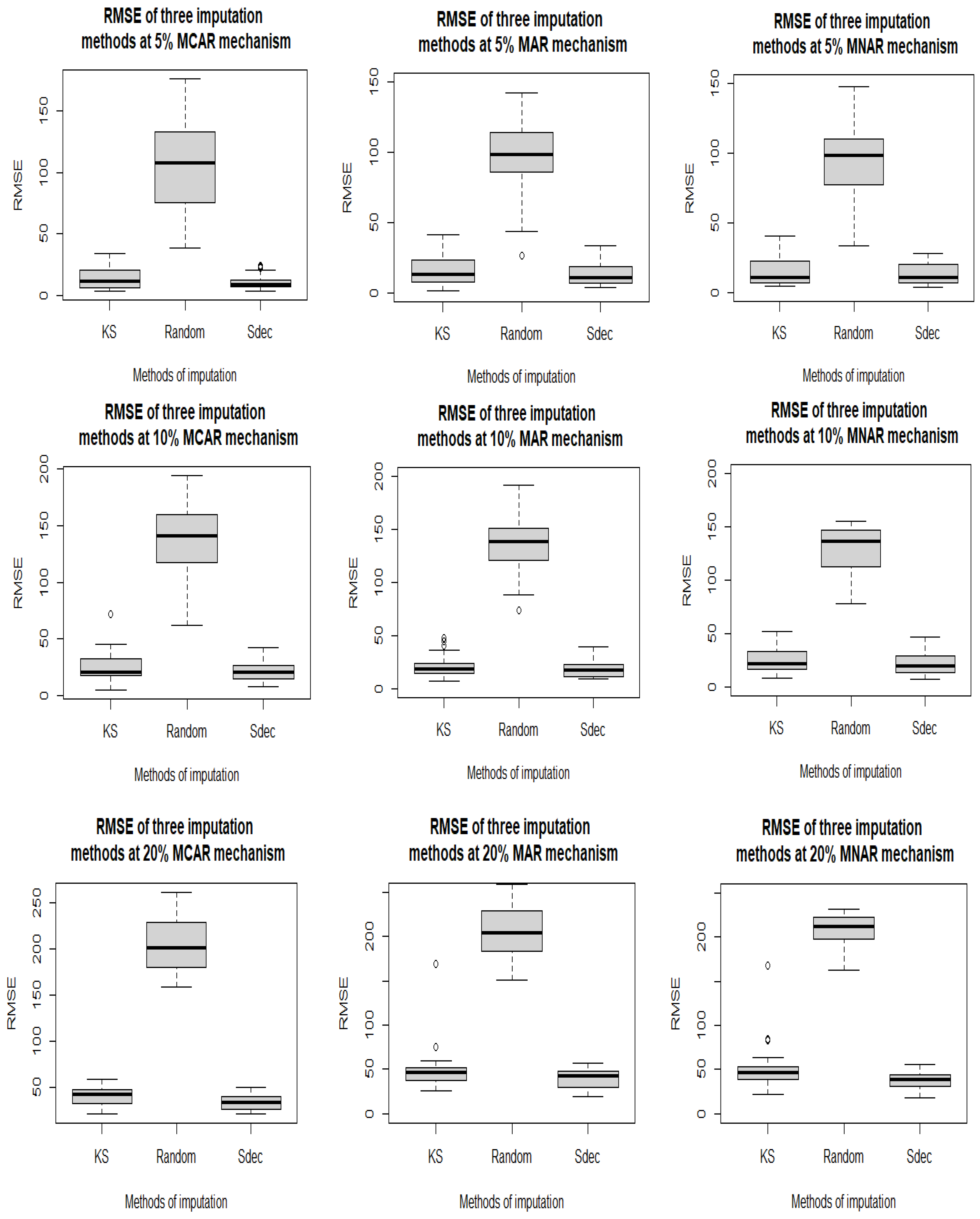
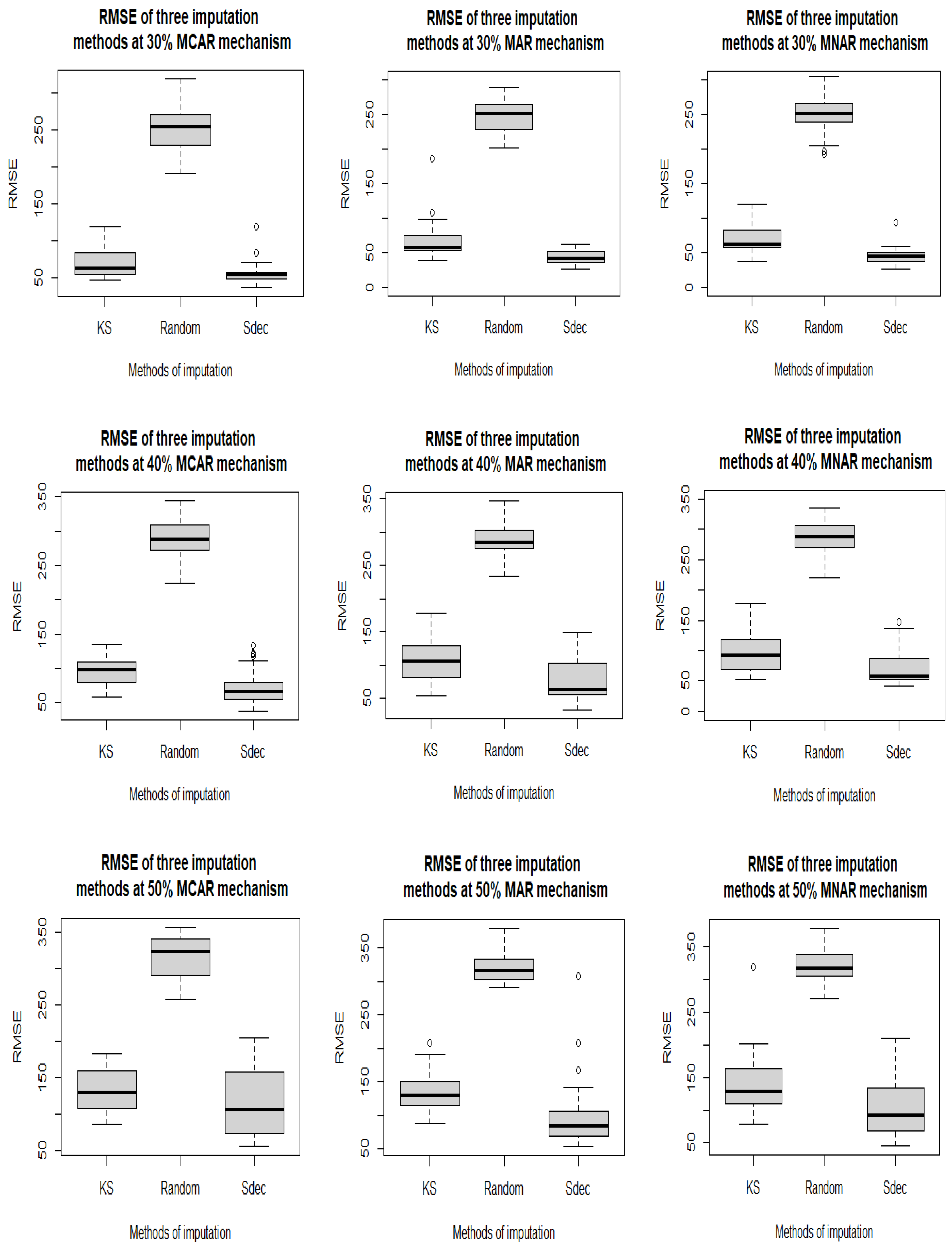
Table 2 shows that the Sdec method is best for imputing missing values for each of the three missing data mechanisms, as it has the lowest (bolded) mean values in each case for all six missingness percentages, followed by the KS and random methods in that order. The random method is always much the worst. See also Figure 3 for boxplots of the results. It is important to note that at lower levels of missingness, especially at 5% and 10%, the KS method (with mean RMSE of 13.61 and 25.36, 16.35 and 22.44, and 15.61 and 25.42, for MCAR, MAR and MNAR mechanisms, respectively) is not much worse than Sdec (which has mean RMSE of 10.46 and 21.22, 13.53 and 19.12, and 13.76 and 22.33, respectively) and the random method comes last. This finding is consistent with the study of Moritz and Bartz-Beielstein [30]. The Sdec method also in most cases has the lowest standard deviation, implying greater consistency than for the other methods; however, at 40% and 50%, the random method seems to be more consistent than the other methods.

The mean RMSE values range between 10.46 and 318.10 for MCAR, 13.53 and 320.50 for MAR and 13.76 and 319.90 for MNAR. These minimum and maximum values for the MCAR mechanism are slightly lower compared to MAR and MNAR. The mean RMSE also increases as the percentage of missingness increases for any method or missing data mechanism, which implies, not surprisingly, that these methods are better when dealing with fewer missing values than at higher levels of missingness.

Figure 3 clearly shows the level and spread of RMSE values at different percentages of missingness, assuming the MCAR, MAR and MNAR mechanisms. For all missingness rates, the values tend to cluster around the median RMSE for both KS and Sdec, especially from 5% to 30%, while the plots for the random method are located higher up and have a wider spread. Again, it is obvious that Sdec is best, based on smaller values of the median RMSE, closely followed by KS, and random is third by some distance. For the random method, the spread in RMSE values tends to decrease as the missing percentage increases, which is similar to the case for the standard deviation values; whereas, for the KS and Sdec methods at higher percentages of missingness, say 40% and 50%, the spread tends to widen and there are some outliers.

The summary of the MAPE statistic in Table 3 also suggests that the best method for imputing missing values at all levels for the Kainji water level discharge is Sdec, the KS method is next best and the random method is poorer. However, as the percentage of missingness in the data increases these differences between the methods become clearer. This can also be seen from the boxplots in Figure S1; however, at 50% missing, Sdec has a wider spread than the other methods, meaning that its MAPE result is more unpredictable at this higher percentage of missing values, similarly to Figure 3. Sdec also has the least variability for 5–30% missingness; whereas, for 40% and 50% missingness, KS generally has the least variability. In this case the MAPE values for the MAR mechanism are the lowest, followed by MCAR and then MNAR. As for RMSE, the mean values increase as the level of missingness increases. For MAPE, the standard deviation values also tend to increase with the level of missingness. Sdec is the best method at 50% missingness, based on the mean RMSE and MAPE, however, it is more variable than KS. Therefore, at that missingness level, KS may be preferred.

3.2. Multivariate Water Level Imputation

The performance of RF, kNN, missForest (MF) and PMM methods, i.e., two single imputation methods (kNN and MF) and two multiple imputation methods (RF and PMM), assuming MCAR, MAR and MNAR missing data mechanisms, were analysed using monthly simulated water level discharge from three water stations, namely Ibi, Makurdi and Umaisha on the river Benue, for the time period 2011–2016, as described above. Five rates of missing values (10%, 20%, 30%, 40% and 50%) were created using the ampute function from the R mice package (results for the 5% missing rate are not included here as it gave fewer points missing for any one station, since the 5% missing values were created across the whole dataset of values for the three stations, and as the results were very similar to those for 10% missingness. The 5% level was initially considered as a low percentage of missing values, for consistency with the univariate study). The missing values were replaced with new values generated from the four methods from the R mice package (RF and PMM), missForest package (MF) and VIM package (kNN).

The accuracies of these four imputation methods were assessed using RMSE and MAPE metrics, using 30 repeats, as above. The mean RMSE for each method at the five missingness levels for the three missingness mechanisms for the three water stations are presented in

Table 4. Comparison of the mean values of the RMSE statistic between the deleted original data and the imputed data for missing completely at random, missing at random and missing not at random mechanisms and the random forest (RF), k nearest neighbour (kNN), missForest (MF) and predictive mean matching (PMM) imputation methods. Values in bold show the best method in each case (with lowest mean).

% Missing	Method	MCAR			MAR			MNAR
		Ibi	Makurdi	Umaisha	Ibi	Makurdi	Umaisha	Ibi	Makurdi	Umaisha
10	RF	22.51	21.24	50.24	21.02	26.02	53.51	25.80	31.33	66.74
	kNN	17.17	16.22	36.61	19.55	15.39	42.42	19.11	19.47	48.17
	MF	14.60	19.24	37.71	17.25	19.13	35.06	20.18	19.67	54.26
	PMM	25.98	24.21	47.57	26.71	25.95	55.31	26.35	24.96	58.47
20	RF	36.81	36.56	81.04	34.71	34.15	85.84	39.21	32.43	76.44
	kNN	23.84	25.51	73.77	28.48	24.92	64.24	32.97	33.66	70.32
	MF	26.76	28.60	62.10	25.00	28.30	56.36	28.22	32.90	76.22
	PMM	33.16	39.17	67.82	34.28	38.65	87.78	41.99	41.25	94.16
30	RF	45.66	47.17	99.47	44.66	43.07	100.85	49.17	43.93	106.59
	kNN	31.86	36.19	79.21	33.11	37.80	74.05	38.69	38.79	83.80
	MF	33.19	39.19	85.16	38.45	35.64	94.59	39.62	39.89	91.93
	PMM	42.01	49.13	103.32	42.58	44.98	97.24	51.59	48.11	115.20
40	RF	49.67	56.49	123.15	51.36	54.03	118.37	50.94	56.74	129.32
	kNN	36.40	46.46	94.26	41.16	43.94	92.94	43.67	46.00	97.40
	MF	39.69	46.75	101.41	36.90	43.16	98.50	46.99	46.30	102.40
	PMM	57.15	61.82	127.80	48.60	63.14	117.17	58.36	55.54	129.24
50	RF	59.70	64.19	136.39	62.00	62.59	139.55	56.40	58.46	147.40
	kNN	44.69	48.28	109.82	45.45	51.10	117.73	49.19	54.01	111.92
	MF	45.76	52.00	106.10	49.49	46.83	106.82	49.75	53.94	111.39
	PMM	61.52	69.37	140.91	57.11	67.09	150.09	66.30	69.90	134.70

and corresponding results for MAPE are shown in

Table 5. Comparison of the mean values of the MAPE statistic between the deleted original data and the imputed data for missing completely at random, missing at random and missing not at random mechanisms and the random forest (RF), k nearest neighbour (kNN), missForest (MF) and predictive mean matching (PMM) imputation methods. Values in bold show the best method in each case (with lowest mean).

% Missing	Method	MCAR			MAR			MNAR
		Ibi	Makurdi	Umaisha	Ibi	Makurdi	Umaisha	Ibi	Makurdi	Umaisha
10	RF	0.0092	0.0062	0.0287	0.0079	0.0081	0.0526	0.0073	0.0070	0.0229
	kNN	0.0062	0.0045	0.0348	0.0075	0.0041	0.0320	0.0055	0.0045	0.0181
	MF	0.0050	0.0054	0.0206	0.0062	0.0057	0.0249	0.0054	0.0043	0.0168
	PMM	0.0094	0.0065	0.0617	0.0111	0.0073	0.0407	0.0060	0.0050	0.0143
20	RF	0.0178	0.0131	0.0877	0.0169	0.0123	0.1907	0.0143	0.0079	0.0232
	kNN	0.0118	0.0094	0.0925	0.0138	0.0087	0.0902	0.0134	0.0104	0.0336
	MF	0.0105	0.0103	0.0507	0.0119	0.0109	0.0610	0.0115	0.0099	0.0273
	PMM	0.0159	0.0155	0.1973	0.0173	0.0133	0.1089	0.0171	0.0122	0.0401
30	RF	0.0255	0.0210	0.1192	0.0266	0.0181	0.1654	0.0228	0.0161	0.0556
	kNN	0.0177	0.0154	0.0967	0.0178	0.0172	0.1260	0.0174	0.0148	0.0396
	MF	0.0206	0.0170	0.1554	0.0230	0.0159	0.1524	0.0191	0.0145	0.0465
	PMM	0.0225	0.0224	0.2060	0.0257	0.0215	0.1519	0.0233	0.0179	0.0927
40	RF	0.0337	0.0271	0.1634	0.0357	0.0270	0.2377	0.0292	0.0242	0.0793
	kNN	0.0239	0.0225	0.1347	0.0282	0.0218	0.1942	0.0233	0.0197	0.0863
	MF	0.0279	0.0238	0.1616	0.0224	0.0218	0.2269	0.0253	0.0195	0.0800
	PMM	0.0388	0.0342	0.1859	0.0330	0.0345	0.2118	0.0352	0.0239	0.1587
50	RF	0.0422	0.0358	0.2513	0.0452	0.0351	0.2330	0.0347	0.0275	0.1258
	kNN	0.0346	0.0251	0.1972	0.0344	0.0286	0.2434	0.0293	0.0257	0.1129
	MF	0.0326	0.0298	0.2098	0.0393	0.0252	0.1895	0.0315	0.0260	0.1061
	PMM	0.0505	0.0425	0.3913	0.0398	0.0376	0.2812	0.0435	0.0344	0.1089

(results for standard deviation are not shown). It was thought that a lower missingness level may have produced lower variability of results, and potentially lower (better) values of the accuracy measures. This is not the case, and from the results for all water stations the variability seems to be similar on the whole for all missing percentages for the methods considered.

From Table 4, for the MCAR mechanism at 10% missingness, the methods with the lowest mean RMSE values are MF, kNN and kNN for the Ibi, Makurdi and Umaisha stations, respectively. At 20% missing, kNN, kNN and MF are best for Ibi, Makurdi and Umaisha, respectively. For 30% and 40% missingness, kNN is the best across all water stations. At 50% missing, the lowest mean RMSE values were for kNN, kNN and MF for Ibi, Makurdi and Umaisha, respectively (see also Figure S2, which shows that kNN and MF tend to have a lower spread around the median RMSE and are overall the best two methods, while PMM and RF tend to have a wider spread and/or be located higher up in the plots for all water stations). For the MAR mechanism at 10% and 20% missing, the best methods are MF, kNN and MF for Ibi, Makurdi and Umaisha, respectively. At 30% missing, kNN, MF and kNN for Ibi, Makurdi and Umaisha, respectively, have the lowest RMSE. For 40% missing, MF, MF and kNN are best, and at 50% missing, kNN, MF and MF are best for the Ibi, Makurdi and Umaisha stations, respectively (Table 4). (Figure S3 also tends to show a lower level and spread around the median RMSE values for MF and kNN, a wider spread for RF and overall PMM is worst). For the MNAR mechanism for 10% missing, kNN is best for all three water stations. At 20% missingness, MF, RF (which is similar to MF in this case) and kNN have the lowest RMSE values for the Ibi, Makurdi and Umaisha stations, respectively. For 30% and 40% missing, kNN is the best method across all water stations. At 50% missingness, RMSE is lowest for kNN, MF and MF for Ibi, Makurdi and Umaisha, respectively (Figure S4 also shows the best two methods as kNN and MF, in that order, and PMM and RF are the worst due to a higher level and spread).

From these results, for the MAR mechanism, MF is generally best, closely followed by kNN, while RF is slightly better overall than PMM, which is last. For the MCAR and MNAR mechanisms, kNN is best, closely followed by MF. There is a clear difference between the best two and the last two imputation methods. RF and PMM are worst. PMM and RF also tend to give a larger spread of RMSE values (Figures S2–S4).

The mean RMSE values range between 14.60 and 140.91 for MCAR, 15.39 and 150.09 for MAR and 19.11 to 147.40 for MNAR, depending on the imputation method and level of missingness, and these values are lowest for the MCAR mechanism compared to MAR and MNAR, which is similar to the conclusion from the univariate case above.

From the summary of the MAPE statistic (Table 5), the overall best method for imputing missing values at all levels of missing data for the three water stations along the river Benue assuming the MCAR mechanism is kNN, followed by MF. RF and PMM are not as good. For the MAR mechanism, MF is best, closely followed by kNN. Finally, MNAR has an interesting result with MF and kNN as the two best methods overall, in that order, while RF is sometimes not far behind, especially at 20% missing, and PMM is generally worst.

The corresponding boxplots for MAPE for the MCAR, MAR and MNAR mechanisms are presented in Figures S5–S7, respectively, and broadly confirm the results for RMSE. These plots do show many high outliers, indicating poor results in some instances, especially for the PMM and RF methods and for the Umaisha water station, but also in some cases for the kNN and MF methods for higher levels of missing data.

4. Discussion

Missing data, especially for hydrological data such as water level data, is a persistent problem for many developing countries for various reasons and ignoring missing data for analysis causes loss of information and potentially misleading conclusions, which in turn impacts mitigating measures taken by governments and other stakeholders. This study compares the performances of several single and multiple imputation methods, each on monthly water level data from the Kainji water station on the river Benue and the Ibi, Makurdi and Umaisha water stations on the river Niger in Nigeria. This aimed to identify the best method(s) for both single and multiple imputation approaches to avoid biased estimates and misleading conclusions [18].

Studies on imputation for missing data in hydrology-related areas have been carried out previously, such as in Gao et al. [10] and Hamzah et al. [40,41]. In Nigeria for instance, using imputation in this area is a new practice. Ekeu-wei et al. [13] introduced the concept of multiple imputation to impute annual peak river discharge, which is vital for flood frequency estimation. Oyerinde et al. [42] used the PMM method to impute missing data from 22 water discharge stations with different missing data percentages. However, these two studies failed to consider the missing data mechanism/pattern, which is important for handling missing data. In addition, they failed to consider single imputation methods, which are frequently suitable for imputing complex univariate time series [30].

For both our univariate and multivariate data, performances of single and multiple imputation methods were compared using RMSE and MAPE statistics. Missingness was introduced in the data at several different rates in each case, using MCAR, MAR and MNAR mechanisms.

For the univariate water level data, of the three single imputation methods considered in this study, the Sdec method is best for imputing the missing data for the three missing data mechanisms. At lower levels of missingness, especially at 5% and 10%, KS is not much worse than Sdec but the random method was much poorer and is not recommended. Furthermore, Sdec in general has the lowest variability in RMSE or MAPE, except at the highest level of missingness. The results for MCAR data were better compared to MCAR or MNAR. However, for univariate time series imputation, assuming MCAR or MAR tends to give similar results [35]. The mean RMSE increases as the percentage of missingness increases, which implies that these methods are better when dealing with fewer missing values, which is not surprising.

For the multivariate case, performances of single and multiple imputation methods were compared. We showed that for MCAR and MAR, missForest has the best results, closely followed by kNN; while, for the MNAR mechanism kNN is the best method, closely followed by missForest; whereas, RF and PMM have low accuracy in imputing data gaps, based on the two performance metrics considered. Coincidently, these two best methods are single imputation methods and are fast to execute, which is also consistent with our findings in the univariate case.

For RF, the random forest method, our study found no consistent improvement in the results as the number of trees increased using the random forest from the mice R package; but, it confirmed that using a large number of trees (say 500) is time consuming and would not be recommended in practice, which is consistent with the finding in Boehmke and Greenwell [66]. For the kNN method, k = 15 and k = 7 consistently produced the best results from either RMSE or MAPE. This conclusion disagrees with the findings of Muinonen et al. [67], who say that imputation accuracy from kNN does not improve for k > 3 but confirm the findings of McRoberts et al. [68] that a higher value of k (k ≥ 7 in our case) may improve estimation accuracy and have a lower variability of results.

This article has examined several imputation methods with water level data for a range of missing value percentages. Clearly, any such study is limited and a wider range of techniques could be used. The focus here is on water levels, and different conclusions may have been drawn with different data. We also considered missing data percentages from very little, at 5%, to a substantial proportion, at 50%, and no higher than 50% as it has been reported that using imputation for datasets with more than 50% missing observations often produces biased results and high variability (unpredictability) in the imputed data [69]. However, Madley-Dowd et al. [70] found that, for data where values are missing according to the missing at random mechanism, imputation can provide unbiased results even with a large percentage of missing data (up to 90% missing). The study in [42] also considered missing data from 2% up to 70% of the dataset size for water discharge data. Therefore, it would be worth examining this further in the context of water level imputation, especially as even in one of the raw datasets (from the Makurdi water station) used to construct the multivariate data 68% of the water levels were missing.

5. Conclusions

Missing values in water level data is a persistent problem, which, if not properly handled before conducting any analysis, may contribute to adverse impacts of extreme events such as flooding, due to loss of information and wrong conclusions and recommendations from the analysis. It is especially common in developing countries. There are various approaches in the literatures aimed at curtailing impacts of data gaps, such as case-wise deletion. Imputation methods allow the direct tackling of data gaps. In this study, single and multiple imputation methods were considered to establish a best approach for missing data for univariate and multivariate water level discharges.

From the univariate analysis, it was concluded that the seasonal decomposition method is best for imputing missing values at various missingness levels for all three missing mechanisms, followed by the Kalman smoothing method. Therefore, the seasonal decomposition method is recommended for imputation in univariate water level data.

For the multivariate analysis, the missForest method was best, followed by kNN for the MCAR and MAR mechanisms, and for the MNAR mechanism, kNN was the best method, closely followed by missForest. The random forest and PMM methods gave poor results based on the two evaluation metrics considered. Both missForest and kNN can be employed to replace missing values in multivariate water level data and are not time consuming to run, unlike random forest imputation.

It would be worthwhile expanding this study to investigate larger percentages of missing data, as missing values are widely encountered in hydrological datasets.

References

- Phan, T.-T.-H.; Nguyen, X.H. Combining statistical machine learning models with ARIMA for water level forecasting: The case of the Red river. Adv. Water Res. 2020, 142, 103656. [Google Scholar] [CrossRef]
- Water Level. Available online: https://www.qmul.ac.uk/chesswatch/water-quality-sensors/water-level/ (accessed on 5 November 2022).
- Khalifeloo, M.H.; Mohammad, M.; Heydari, M. Multiple imputation for hydrological missing data by using a regression method (Klang River Basin). Int. J. Res. Eng. Technol. 2015, 4, 519–524. [Google Scholar]
- Elshorbagy, A.; Simonovic, S.; Panu, U. Estimation of missing streamflow data using principles of chaos theory. J. Hydrol. 2002, 255, 123–133. [Google Scholar] [CrossRef]
- Ramirez, S.G.; Williams, G.P.; Jones, N.L. Groundwater level data imputation using machine learning and remote earth observations using inductive bias. Remote Sens. 2022, 14, 5509. [Google Scholar] [CrossRef]
- Little, R.J.A. Missing-data adjustments in large surveys. J. Bus. Econ. Stat. 1988, 6, 287–296. [Google Scholar] [CrossRef]
- Zhang, Y.; Thorburn, P.J. Handling missing data in near real-time environmental monitoring: A system and a review of selected methods. Fut. Generat. Comput. Syst. 2022, 128, 63–72. [Google Scholar] [CrossRef]
- Twala, B. An empirical comparison of techniques for handling incomplete data using decision trees. Appl. Artific. Intellig. 2009, 23, 373–405. [Google Scholar]
- Regonda, S.K.; Seo, D.-J.; Lawrence, B.; Brown, J.D.; Demargne, J. Short-term ensemble streamflow forecasting using operationally-produced single-valued streamflow forecasts—A Hydrologic Model Output Statistics (HMOS) approach. J. Hydrol. 2013, 497, 80–96. [Google Scholar] [CrossRef]
- Gao, Y.; Merz, C.; Lischeid, G.; Schneider, M. A review on missing hydrological data processing. Environ. Earth Sci. 2018, 77, 47. [Google Scholar] [CrossRef]
- Plaia, A.; Bondì, A.L. Single imputation method of missing values in environmental pollution datasets. Atmosp. Environ. 2006, 40, 7316–7330. [Google Scholar] [CrossRef]
- Guzman, J.A.; Moriasi, D.; Chu, M.; Starks, P.; Steiner, J.; Gowda, P. A tool for mapping and spatio-temporal analysis of hydrological data. Environ. Model. Softw. 2013, 48, 163–170. [Google Scholar] [CrossRef]
- Ekeu-wei, I.T.; Blackburn, G.A.; Pedruco, P. Infilling Missing Data in Hydrology: Solutions Using Satellite Radar Altimetry and Multiple Imputation for Data-Sparse Regions. Water 2018, 10, 1483. [Google Scholar] [CrossRef] [Green Version]
- Chung, S.Y.; Venkatramanan, S.; Elzain, H.E.; Selvam, S.; Prasanna, M.V. Supplement of missing data in groundwater-level variations of peak type using geostatistical methods. In GIS and Geostatistical Techniques for Groundwater Science, 1st ed.; Venkatramanan, S., Prasanna, M.V., Chung, S.Y., Eds.; Elsevier: Amsterdam, The Netherlands, 2019; pp. 33–41. [Google Scholar] [CrossRef]
- Zhang, Y.; Thorburn, P.J.; Xiang, W.; Fitch, P. SSIM—A deep learning approach for recovering missing time series sensor data. IEEE Internet Things J. 2019, 6, 6618–6628. [Google Scholar] [CrossRef]
- Gires, A.; Tchiguirinskaia, I.; Schertzer, D. Infilling missing data of binary geophysical fields using scale invariant properties through an application to imperviousness in urban areas. Hydrol. Sci. J. 2021, 66, 1197–1210. [Google Scholar] [CrossRef]
- Norazian, M.N.; Shukri, Y.A.; Azam, R.N.; Al Bakri, A.M.M. Estimation of missing values in air pollution data using single imputation techniques. Sci. Asia 2008, 34, 341–345. [Google Scholar] [CrossRef]
- Kang, H. The prevention and handling of the missing data. Korean J. Anesthesiol. 2013, 64, 402–406. [Google Scholar] [CrossRef] [Green Version]
- Soley-Bori, M. (Boston University, Boston, United States); Dealing with Missing Data: Key Assumptions and Methods for Applied Analysis. 2013. Available online: https://www.bu.edu/sph/files/2014/05/Marina-tech-report.pdf (accessed on 22 October 2021).
- Peugh, J.L.; Enders, C.K. Missing data in educational research: A review of reporting practices and suggestions for improvement. Rev. Educ. Res. 2004, 74, 525–556. [Google Scholar] [CrossRef]
- Cool, A.L. (Texas A&M University, Texas, United States) A Review of Methods for Dealing with Missing Data. 2000. Available online: https://files.eric.ed.gov/fulltext/ED438311.pdf (accessed on 2 December 2022).
- Enders, C.K. Applied Missing Data Analysis, 1st ed.; Guilford Press: New York, NY, USA, 2010. [Google Scholar]
- Graham, J.W.; Hofer, S.M. Multiple imputation in multivariate research. In Modeling Longitudinal and Multilevel Data: Practical Issues, Applied Approaches, and Specific Examples; Little, T.D., Schnabel, K.U., Baumert, J., Eds.; Lawrence Erlbaum Associates Publishers: Hillsdale, NJ, USA, 2000; pp. 201–218. [Google Scholar]
- Little, R.J.A.; Rubin, D.B. Statistical Analysis with Missing Data, 1st ed.; John Wiley & Sons: Hoboken, NJ, USA, 1987. [Google Scholar]
- Arnab, R. Survey Sampling Theory and Applications, 1st ed.; Academic Press: London, UK, 2017. [Google Scholar]
- Zhang, Z. Missing data imputation: Focusing on single imputation. Ann. Translat. Med. 2016, 4, 1–9. [Google Scholar] [CrossRef]
- Saunders, J.A.; Morrow-Howell, N.; Spitznagel, E.; Doré, P.; Proctor, E.K.; Pescarino, R. Imputing missing data: A comparison of methods for social work researchers. Soc. Work Res. 2006, 30, 19–31. [Google Scholar] [CrossRef]
- Rubin, D.B. Multiple imputations in sample surveys: A phenomenological Bayesian approach to nonresponse (with discussion). In Proceedings of the American Statistical Association, Alexandria, VA, USA, 8–10 March 1978; Available online: http://www.asasrms.org/Proceedings/papers/1978_004.pdf (accessed on 1 December 2022).
- Little, R.J.A.; Rubin, D.B. Statistical Analysis with Missing Data, 2nd ed.; John Wiley & Sons: Hoboken, NJ, USA, 2002. [Google Scholar]
- Moritz, S.; Bartz-Beielstein, T. imputeTS: Time series missing value imputation in R. R. J. 2017, 9, 207–218. Available online: https://cran.r-project.org/web/packages/imputeTS/vignettes/imputeTS-Time-Series-Missing-Value-Imputation-in-R.pdf (accessed on 28 October 2021). [CrossRef] [Green Version]
- Wijesekara, W.; Liyanage, L. Comparison of Imputation Methods for Missing Values in Air Pollution Data: Case Study on Sydney Air Quality Index. In Proceedings of the Advances in Information and Communication, Future of Information and Communication Conference (FICC), San Francisco, CA, USA, 5–6 March 2020. [Google Scholar] [CrossRef]
- Chandrasekaran, S.; Moritz, S.; Zaefferer, M.; Stork, J.; Bartz-Beielstein, T.; Bartz-Beielstein, T. Data Preprocessing: A New Algorithm for Univariate Imputation Designed Specifically for Industrial Needs. In Proceedings of the Workshop on Computational Intelligence, Dortmund, Germany, 24–25 November 2016. [Google Scholar]
- Demirhan, H.; Renwick, Z. Missing value imputation for short to mid-term horizontal solar irradiance data. Appl. Energy 2018, 225, 998–1012. [Google Scholar] [CrossRef]
- Afrifa-Yamoah, E.; Mueller, U.A.; Taylor, S.M.; Fisher, A.J. Missing data imputation of high-resolution temporal climate time series data. Meteor. Appl. 2020, 27, 1–18. [Google Scholar] [CrossRef] [Green Version]
- Moritz, S.; Sardá, A.; Bartz-Beielstein, T.; Zaefferer, M.; Stork, J. Comparison of different methods for univariate time series imputation in R. arXiv 2015. [Google Scholar] [CrossRef]
- Jadhav, A.; Pramod, D.; Ramanathan, K. Comparison of performance of data imputation methods for numeric dataset. Appl. Artif. Intel. 2019, 33, 913–933. [Google Scholar] [CrossRef]
- Alsaber, A.; Al-Herz, A.; Pan, J.; AL-Sultan, A.T.; Mishra, D.; KRRD Group. Handling missing data in a rheumatoid arthritis registry using random forest approach. Int. J. Rheum. Dis. 2021, 24, 1282–1293. [Google Scholar]
- Alsaber, A.; Pan, J.; Al-Hurban, A. Handling complex missing data using random forest approach for an air quality monitoring dataset: A case study of Kuwait environmental data (2012 to 2018). Int. J. Environ. Res. Public Health 2021, 18, 1333. [Google Scholar] [CrossRef]
- Ben Aissia, M.A.; Chebana, F.; Ouarda, T.B.M.J. Multivariate missing data in hydrology—Review and applications. Adv. Water Res. 2017, 110, 299–309. [Google Scholar] [CrossRef] [Green Version]
- Hamzah, F.B.; Hamzah, F.M.; Razali, S.F.M.; Samad, H. A comparison of multiple imputation methods for recovering missing data in hydrological studies. Civil Eng. J. 2021, 7, 1608–1619. [Google Scholar] [CrossRef]
- Hamzah, F.B.; Hamzah, F.M.; Razali, S.F.M.; El-Shafie, A. Multiple imputations by chained equations for recovering missing daily streamflow observations: A case study of Langat River basin in Malaysia. Hydrol. Sci. 2022, 67, 137–149. [Google Scholar] [CrossRef]
- Oyerinde, G.T.; Lawin, A.E.; Adeyeri, O.E. Multi-variate infilling of missing daily discharge data on the Niger basin. Water Pract. Techno. 2021, 16, 961–979. [Google Scholar] [CrossRef]
- Little, R.J.A.; Rubin, D.B. Statistical Analysis with Missing Data, 3rd ed.; John Wiley & Sons: Hoboken, NJ, USA, 2019. [Google Scholar]
- Santos, M.S.; Pereira, R.C.; Costa, A.F.; Soares, J.P.; Santos, J.; Abreu, P.H. Generating Synthetic Missing Data: A Review by Missing Mechanism. IEEE Access 2019, 7, 11651–11667. [Google Scholar] [CrossRef]
- Welch, G.; Bishop, G. An Introduction to the Kalman Filter. In Technical Report TR 95–041; Department of Computer Science, University of North Carolina: Chapel Hill, NC, USA, 1995. [Google Scholar]
- Maybeck, P.S. Chapter 1 Introduction. In Stochastic Models Estimation and Control (Mathematics in Science and Engineering); Maybeck, P.S., Ed.; Academic Press: London, UK, 1979; pp. 1–24. [Google Scholar]
- Durbin, J.; Koopman, S.J. Time Series Analysis by State Space Methods, 2nd ed.; Oxford University Press: Oxford, UK, 2012. [Google Scholar]
- Fulton, C.T. Sectoral Prices and Price-Setting. Ph.D Thesis, University of Oregon, Eugene, OR, USA, 2016. [Google Scholar]
- Cleveland, R.B.; Cleveland, W.S.; McRee, J.E.; Terpenning, I. STL: A seasonal-trend decomposition procedure based on loess. J. Off. Stat. 1990, 6, 3–33. [Google Scholar]
- Eskelson, B.N.; Temesgen, H.; Lemay, V.; Barrett, T.M.; Crookston, N.L.; Hudak, A.T. The roles of nearest neighbor methods in imputing missing data in forest inventory and monitoring databases. Scand. J. For. Res. 2009, 24, 235–246. [Google Scholar] [CrossRef] [Green Version]
- Kowarik, A.; Templ, M. Imputation with the R Package VIM. J. Stat. Softw. 2016, 74, 1–16. [Google Scholar] [CrossRef] [Green Version]
- Chen, J.; Shao, J. Nearest neighbor imputation for survey data. J. Off. Stats. 2000, 16, 113–131. [Google Scholar]
- Gower, J.C. A general coefficient of similarity and some of its properties. Biometrics 1971, 27, 857–871. [Google Scholar] [CrossRef]
- Rubin, D.B. Statistical matching and file concatenation with adjusted weights and multiple imputations. J. Bus. Econ. Stats. 1986, 4, 87–94. [Google Scholar] [CrossRef]
- van Buuren, S.; Groothuis-Oudshoorn, K. mice: Multivariate Imputation by Chained Equations in R. J. Stat. Softw. 2011, 45, 1–67. [Google Scholar] [CrossRef] [Green Version]
- Breiman, L. Random forests. Mach. Learn. 2001, 45, 5–32. [Google Scholar] [CrossRef] [Green Version]
- Introduction to Random Forest in Machine Learning. Available online: https://www.section.io/engineering-education/introduction-to-random-forest-in-machine-learning/ (accessed on 2 November 2022).
- Stekhoven, D.J.; Buehlmann, P. MissForest-nonparametric missing value imputation for mixed-type data. Bioinformatics 2012, 28, 112–118. [Google Scholar] [CrossRef] [Green Version]
- Doove, L.L.; Van Buuren, S.; Dusseldorp, E. Recursive partitioning for missing data imputation in the presence of interaction effects. Comput. Stats. Data Anal. 2014, 72, 92–104. [Google Scholar] [CrossRef]
- Hong, S.; Lynn, H. Accuracy of random-forest-based imputation of missing data in the presence of non-normality, non-linearity, and interaction. BMC Med. Res. Methodol. 2020, 20, 199. [Google Scholar] [CrossRef] [PubMed]
- Tang, F.; Ishwaran, H. Random forest missing data algorithms. statistical analysis data mining. ASA Data Sci. J. 2017, 10, 363–377. [Google Scholar] [CrossRef]
- Ramosaj, B.; Pauly, M. Predicting missing values: A comparative study on nonparametric approaches for imputation. Computing 2019, 34, 1741–1764. [Google Scholar] [CrossRef]
- Solaro, N.; Barbiero, A.; Manzi, G.; Ferrari, P.A. A simulation comparison of imputation methods for quantitative data in the presence of multiple data patterns. J. Stats. Comput. Sim. 2018, 88, 588–619. [Google Scholar] [CrossRef]
- Chai, T.; Draxler, R.R. Root mean square error (RMSE) or mean absolute error (MAE)?—Arguments against avoiding RMSE in the literature. Geosci. Model Devel. 2014, 7, 1247–1250. [Google Scholar] [CrossRef] [Green Version]
- De Myttenaere, A.; Golden, B.; Le Grand, B.; Rossi, F. Mean absolute percentage error for regression models. Neurocomputing 2016, 192, 38–48. [Google Scholar] [CrossRef] [Green Version]
- Boehmke, B.; Greenwell, B.M. Hands-On Machine Learning with R, 1st ed.; CRC Press: New York, NY, USA, 2019. [Google Scholar] [CrossRef]
- Muinonen, E.; Maltamo, M.; Hyppänen, H.; Vainikainen, V. Forest stand characteristics estimation using a most similar neighbor approach and image spatial structure information. Remote Sens. Environ. 2001, 78, 223–228. [Google Scholar] [CrossRef]
- McRoberts, R.E.; Nelson, M.D.; Wendt, D.G. Stratified estimation of forest area using satellite imagery, inventory data, and the k-nearest neighbors technique. Remote Sens. Environ. 2002, 82, 457–468. [Google Scholar] [CrossRef]
- Clavel, J.; Merceron, G.; Escarguel, G. Missing data estimation in morphometrics: How much is too much? Syst. Biol. 2014, 63, 203–218. [Google Scholar] [CrossRef]
- Madley-Dowd, P.; Hughes, R.; Tilling, K.; Heron, J. The proportion of missing data should not be used to guide decisions on multiple imputation. J. Clin. Epidem. 2019, 110, 63–73. [Google Scholar] [CrossRef] [PubMed] [Green Version]
Figure 1.
Map of Nigeria showing the four water stations (marked left to right as follows by symbols: Kainji (star), Umaisha (small square), Makurdi (diamond), Ibi (circle)) along the rivers Benue and Niger (source: Google Maps, modified by authors).
Figure 2.
A decision tree and its three different types of nodes.
Figure 3.
Boxplots of RMSE values for Kalman smoothing (KS), random and seasonal decomposition (Sdec) methods at 5%, 10%, 20%, 30%, 40%, and 50% levels of missingness, respectively, for the missing completely at random (MCAR), missing at random (MAR) and missing not at random (MNAR) missing value mechanisms.