On ST6 Source Terms Model Assessment and Alternative

Abstract

We present the study of the ST6 balanced set of wind energy input and wave energy dissipation due to wave breaking source terms, offered as the option in operational wave forecasting models and based on theoretical self-similarity analysis and numerical simulation of the wave energy radiative transfer equation. The study relies on the classical limited fetch wind wave excitation problem with constant wind blowing orthogonally to the shoreline toward the open ocean. It is found that the ST6 model exhibits asymptotic quasi self-similar behavior for fetches exceeding $\simeq 25$ km, as well as non-universal wave energy growth for shorter fetches, depending on the shoreline wave energy levels. We construct the alternative model PGZ-2 from a self-similar consideration, which reproduces field experimental data almost in the whole fetch span and reduces wave energy evolution dependence on the shoreline energy level. We assert that the PGZ-2 model is more accurate than the ST6 model. Moreover, it has a wider area of applicability.

1. Introduction

The study of ocean waves is significant in many ways. First, waves are one of the main mechanisms of interaction between air and water. As such, they determine the effect of the ocean on the weather (both locally and globally) as well as the weather effect on the ocean motion. The impact of the ocean on the Earth’s climate cannot be overestimated. Another important field is the study of the waves themselves. This is of great value for ship navigation, coastal construction, and other fields.

It is widely accepted nowadays that [1,2] the wave kinetic equation based on slowly changing wave amplitude (WKB approximation), also known in physical oceanography as the radiative transfer equation [3], statistically describes the evolution of nonlinear ocean surface waves:

$$\begin{array}{c}\hfill \frac{\partial \epsilon }{\partial t}+\frac{\partial \omega }{\partial \mathbf{k}}\frac{\partial \epsilon }{\partial \mathbf{r}}=S_{\mathrm{nl}}+S_{\mathrm{in}}+S_{\mathrm{ds}}\end{array}$$

(1)

where $\epsilon (k,\theta ,\mathbf{r},t)$ is the wave energy spectral density, $\mathbf{r}=\mathbf{r}(x,y)$ and $\mathbf{k}=(k,\theta )$ are the real space vector coordinate and Fourier space wave vector, k and $\theta$ are the modulus of the wave number and the angle of wave propagation, $\omega =\sqrt{kg}$ is deep water dispersion relation, and g is the gravity acceleration. $S_{\mathrm{nl}}$, $S_{\mathrm{in}}$, and $S_{\mathrm{ds}}$ are the nonlinear wave interaction, the wind energy input, and the dissipation source terms, respectively.

For more than 40 years, significant efforts have been devoted to the construction of different forms of $S_{\mathrm{in}}$ and $S_{\mathrm{ds}}$. In the current research, we are focusing on the assessment of recently developed ST6 wind energy input $S_{\mathrm{in}}^{\mathrm{ST}6}$ and wave energy dissipation $S_{\mathrm{ds}}^{\mathrm{ST}6}$ source terms, recently included as a package in the operational wave forecasting model WAVEWATCH III [4].

The ST6 model history originates from 3-year experimental observations, performed in Lake George, Australia, from 1997 through 2000 by [5,6]. These measurements resulted in several conclusions, including that $S_{\mathrm{in}}$ is the nonlinear function of the spectrum. For the wave-breaking dissipation, the conclusion of the threshold existence for “inherent” wave-breaking has been made in terms of “significant” wave steepness. Additionally, the opinion regarding the existence of the “two-phase” behavior of wave dissipation has been expressed: the wave-breaking can be realized at any scale, but for the above spectral peak waves, the breaking is enhanced due to the compression of the shorter waves by the longer ones.

Conceptually, a different approach to the formulation of wind energy input and wave breaking dissipation source terms, based on self-similar properties of Equation (1) and known as ZRP balanced source terms model, has been recently realized in [7,8]. It relied on the self-similar solutions of Equation (1) with the “footprints” in the form of specific indices of power-like total energy and mean frequency dependencies on the fetch, predicted theoretically by Zakharov with co-authors [9,10,11] and observed in multiple field experiments analyzed in [12]. It was also shown in [7] that out of five numerically tested historically known wind energy input source terms with similar wave dissipation, four exhibited complete or quasi self-similar behavior, and one failed the self-similarity test. Thus, self-similarity is a well-known ocean surface wave property, confirmed experimentally [13] as well as numerically [14] but generally overlooked in applications.

In the current paper, we are applying the above-mentioned self-similarity testing technology [7] to ST6 source terms model. The comparison, performed with respect to the numerical results from [15] and with earlier work by Gagnaire-Renou et al. [16] detects the fetch span, where quasi-self-similar behavior is realized. Motivated by these observations, we propose an alternative source terms model, abbreviated to PGZ-2, which improves the ST6 model properties demonstrated in [15].

The kinetic equation of type (1) is a well-establish basis for the study of wave spectra. Nevertheless, one should remember that such an approach has its restrictions which arise from the fact that the kinetic equation is an approximation and neglects some correlation properties of the nonlinear waves [17]. In our article, we deal with the conventional Hasselmann equation as the base of our model; the real ocean may be more complex.

As the PGZ-2 model is still in development, in this paper we present the application of the model to the steady wave solution and perform the comparison of the model to the ST6 one.

2. Materials and Methods

2.1. Numerical Models

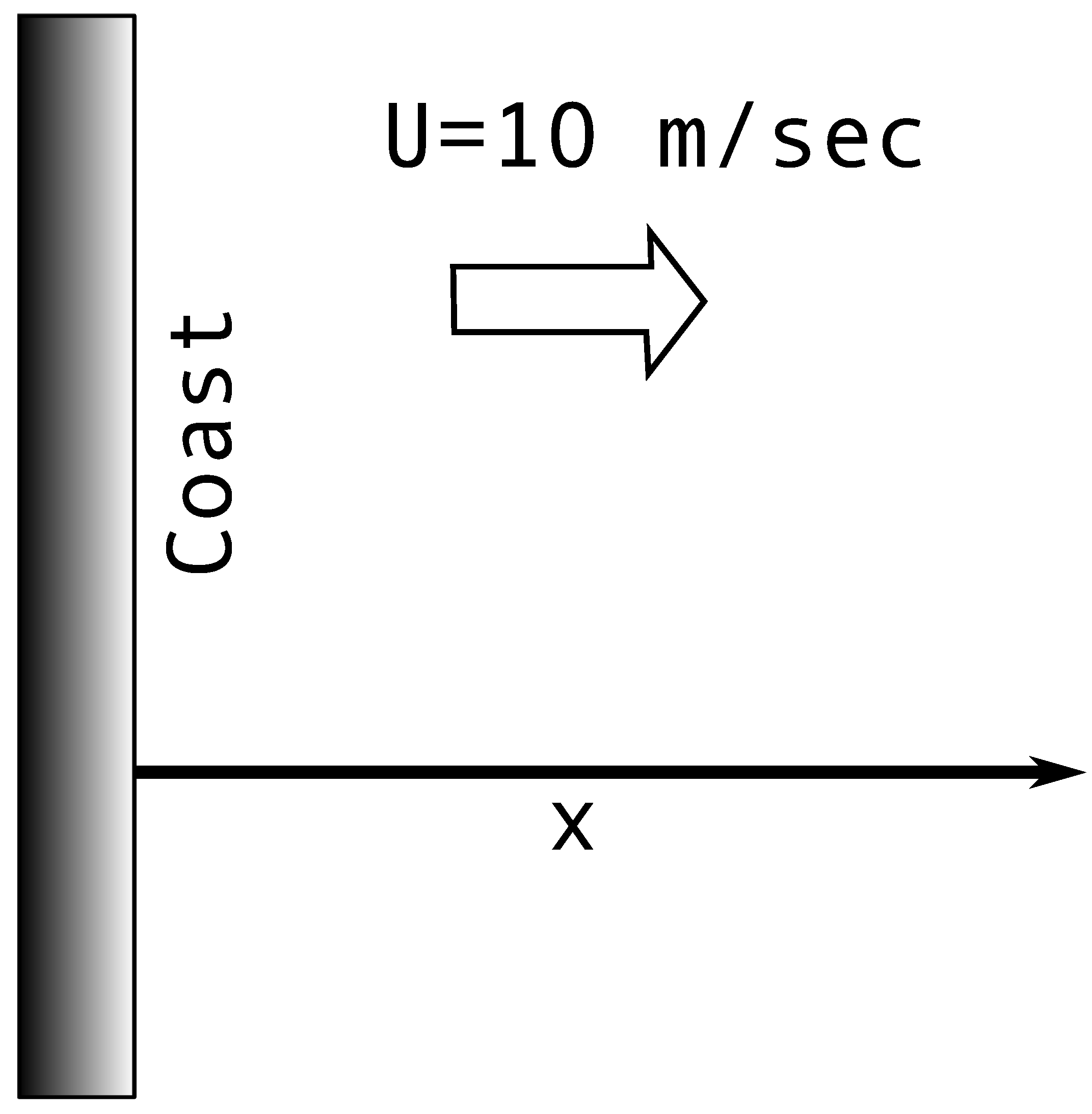
Recently, the full version of Equation (1) has been modeled in the limited fetch statement [15] with constant offshore wind of 10 m/s orthogonally to the fetch (Figure 1) in the framework of the WAVEWATCH III operational model. This was an extremely difficult computational problem, first and foremost, due to the necessity of the calculation of the exact nonlinear wave interaction in every real-space 2D grid point on every time step. See [15] for the details.

In the presented research, the simplified and much more computationally easy approach has been used. We considered the stationary version of Equation (1) in limited fetch formulation:

$$\begin{array}{c}\hfill \frac{1}{2}cos\theta \frac{\omega }{k}\frac{\partial \epsilon }{\partial x}=S_{\mathrm{nl}}+S_{\mathrm{in}}+S_{\mathrm{ds}}\end{array}$$

(2)

used for numerical simulations by [7,8,18]. These works utilized the full four-wave interaction term $S_{\mathrm{nl}}$, calculated with the help of WRT algorithm by [19,20]. The first order forward spatial derivative numerical scheme in the fetch coordinate has been used for the integration of the Equation (2) but led to the appearance of quasi-monochromatic waves in the direction orthogonal to the wind observed in the numerical experiments of [21,22,23,24] as well as the field observations by [25,26,27,28,29,30,31]. The appearance of quasi-monochromatic waves orthogonal to the wind and leading eventually to the numerical instability was circumvented in the publications of [7,8,18] through zeroing of one-half of the Fourier space corresponding to the waves running in the wind direction. The absence of such truncation of phase space for waves, running against and orthogonal to the wind, leads to the eventual blow-up in the numerical simulation of Equation (2).

The advantage of the described approach consists in the fact that the described model with truncated nonlinear wave interactions uses significantly finer spatial resolution step of just 1 meter for the the whole fetch span. At the same time, the disadvantage of this approach is neglect of wind-opposite and wind-orthogonal wave generation. Nevertheless, this type of approach has, apparently, the physical sense. The first reason to believe in such approximation is the initial development of the wave propagation in the form of combined self-similar solutions for fetch-limited and duration-limited situations [22,23]. The second reason consists in the fact that in the asymptotic state, observed in Pushkarev [21], Pushkarev and Zakharov [22], Pushkarev [23], the self-similar structure is preserved for most of the waves running in the wind direction, and finally, the third reason consists in the tendency of the appearance of waves in the direction “almost orthogonal” to the wind, even in the truncated version of the wave model Equation (2).

2.2. Theoretical Background: Self-Similar Solutions

For the reader’s convenience, we repeat self-similar aspects of wave ensemble behavior studied in [8,32]. The equation

$$\frac{1}{2}\frac{\omega }{k}cos\theta \frac{\partial ϵ}{\partial x}=S_{\mathrm{nl}}+S_{\mathrm{in}}$$

(3)

allows self-similar substitution

$$\begin{array}{c}\hfill \epsilon (\omega ,\theta ,x)=x^{p+q}F(\omega x^q,\theta )\end{array}$$

(4)

subject to the relations

$$\begin{array}{ccc}& & 10q-2p=1\hfill \end{array}$$

(5)

$$\begin{array}{ccc}& & q=\frac{1}{2+s}\hfill \end{array}$$

(6)

Equation (5) is known as the “magic relation”. The self-similar behavior of the wave ensemble can be identified through the simple test: if the integral characteristics of the wave ensemble have power-like dependencies on the fetch, i.e., total wave energy $E\sim x^p$ and mean frequency $<\omega >\sim x^{-q}$, and the indices p and q satisfy the relation (5), then the system behavior is self-similar.

The spectrum shape is mostly defined by the nonlinear interactions which are governed by the Hasselmann equation. Such a situation allows for self-similar solutions which scale both in frequency scale and in energy value. Those scalings are connected to each other.

The system of Equations (5) and (6) do not define values of p, q, and s, since it needs the third relation, which can be taken from the experimental field observations. This procedure has been performed in [8], where it was taken in the form of the regression line for the specific spectral characteristic of the experimental field measurements [8], allowing the finding of the set of values

$$\begin{array}{c}\hfill p=1,q=0.3,s=\frac{4}{3}\end{array}$$

(7)

which define the so-called ZRP wind input term.

Below, we will perform a different task: knowing target field experimental relation index p, we will demonstrate that it is possible to come up with the specific value of s, allowing us to build the new model, reproducing and improving partial quasi-self-similar properties of the ST6 model.

Still, this task is not straightforward. The reason is that there is an initial stage of wave turbulence development which is not self-similar. Therefore, the value of s obtained with the help of Equation (6) would be an estimate. Nevertheless, it can be used as the first approximation. Further tuning is required to obtain the newly constructed source term model.

2.3. Theoretical Background: Nonlinear Interactions

The nonlinear interactions are governed by Hasselmann equation [33], which is the kinetic equation for wave modes of different frequencies and directions exchanging energy by nonlinear interactions.

$$\begin{array}{c}{S}_{\mathrm{nl}}=\pi g^2\underset{{\mathbf{k}}_2,{\mathbf{k}}_3,{\mathbf{k}}_4}{\int }{T}^2\left(N{N}_3{N}_4+N_2{N}_3{N}_4-N{N}_2{N}_3-N{N}_2{N}_4\right)\times \\ \times \delta (\omega +{\omega }_2-{\omega }_3-{\omega }_4)\delta (\mathbf{k}+{\mathbf{k}}_2-{\mathbf{k}}_3-{\mathbf{k}}_4)d{\mathbf{k}}_{2}d{\mathbf{k}}_{3}d{\mathbf{k}}_4\end{array}$$

(8)

Here, $N\left(\mathbf{k}\right)$ is the wave number spectrum (the wave number is the wave motion invariant connected to energy spectrum as $\epsilon =\omega N$), $\omega$ is the angular frequency (for deep water waves $\omega =\sqrt{gk}$), g is the gravity acceleration, $\mathbf{k}$ is the wave vector. The nonlinear interaction rate is defined by the coupling coefficient T. The equation includes two $\delta$-functions which describe the resonances required for the waves to interact. The resonances are both in space (wave vectors $\mathbf{k}$) and in time (frequencies $\omega$). Note that the 3-wave resonances are impossible for gravity surface waves because of their dispersion condition. This is why the interaction is through 4-wave interaction. The relative smallness of this interaction provides for the ability to deal with wave modes independently (so called “weak turbulence”).

To calculate the spectra evolution, the new algorithm was used. This algorithm is based on the pre-configured grid of the interacting 4-wave quadruplets. The grid was chosen based on different quadruplet significance with the emphasis on the quadruplets near the center of the so-called Phillips curve. Those quadruplets carry the majority of the energy transfer.

The quadruplet interaction uses quadruplets satisfying the resonance condition:

$$\begin{array}{c}\hfill {\omega }_1+{\omega }_2={\omega }_3+{\omega }_4\\ \hfill {\mathbf{k}}_1+{\mathbf{k}}_2={\mathbf{k}}_3+{\mathbf{k}}_4\end{array}$$

(9)

The exact obedience of the resonance condition for each quadruplet ensures energy conservation, preventing error accumulation. As the quadruplet vectors do not coincide exactly with the grid points of the energy spectrum, we have to use the bilinear interpolation to determine the spectrum value at each quadruplet vector. Still, energy conservation is ensured by the calculation algorithm which specifically maintains that nonlinear interactions result only in redistribution of the energy.

The use of the quadruplet grid allows for easy parallelization of the calculations. The interaction for each quadruplet may be calculated independently, and therefore, each processor core may be used for the calculation of some part of the quadruplet grid without any loss of the processor time.

The backward scattering presents another problem in calculations. We use a small initial wave spectrum near the coast as the boundary condition. The wind pumping produces mostly the forward waves (which propagate from the coast to the open ocean). The nonlinear interaction mostly keeps this outward direction. Therefore, to simplify the calculation, we ignored the waves which are directed towards the coast. When doing the calculations, we manually zeroed that part of the spectra at each numerical step.

The significant part of the model is the high-frequency tail addition for the energy spectrum. Both the ST6 and PGZ-2 models include, together with the pumping, some kind of energy dissipation, but the main part of the energy pumped stays in the energy spectrum. This energy is being transferred from the lower frequencies to the high frequencies by the Kolmogorov cascade transfer, which results in the formation of Zakharov–Filonenko spectrum [34]. This spectrum has $\epsilon \sim {\omega }^4$ with the energy transfer proportional to the energy scale in the 3rd power. The numerical calculations may cover only some part of the frequency scale, and the the energy transfer outside this part is unavoidable. Thus, one needs to provide for some kind of continuation.

O. Phillips in [35] suggested another form of the spectral tail, namely

$$E\left(\omega \right)=\frac{\alpha g^2}{{\omega }^5}$$

(10)

Here, $\alpha \simeq 0.0081$ is the universal Phillips constant. This asymptotic is observed for the utmost high frequency area, while in the energy capacity spectral band, the ZF spectrum is realized.

We use the classic Phillips spectrum as the tail which we added artificially outside the numerical calculation zone.

2.4. ST6 Model Numerical Simulation

We reproduced the numerical experiments, performed in the frame of full model Equation (1) in [15], using truncated model Equation (2). Numerical experiments of [15] targeted the field experimental benchmark for the total dimensionless wave energy dependence on the fetch [36], hereafter KC1992:

$$\begin{array}{ccc}& & {\epsilon }_{*}=\frac{H_s^2{g}^2}{16u_{*}^4}=2.1·{10}^{-3}{\chi }_{*}^{0.79}\hfill \end{array}$$

(11)

where $H_s=4\sqrt{E}$ is significant wave height, E is the total energy, ${\chi }_{*}=gx/u_{*}^2$ is dimensionless fetch, $u_{*}=U_{10}/\mathrm{\Gamma }$ is friction velocity, and $\mathrm{\Gamma }=31$. Omitting the details of the ST6 model, we present the following tuning parameters of the ST6 source terms, described in detail in Liu et al. [15] for WRT nonlinear interaction case:

$$\begin{array}{ccc}& & a_0=0.05,{\mu }_1=2.8,{\mu }_2=1.0,{\mu }_3=10.,{\mu }_4=11.\hfill \\ & & p_1=p_2=4,a_1=4.75·{10}^{-6},a_2=7.00·{10}^{-5}\hfill \end{array}$$

The presented numerical results were obtained using this parameters set.

We present our set of parameters value below at the Section 3 (see Equation (16)).

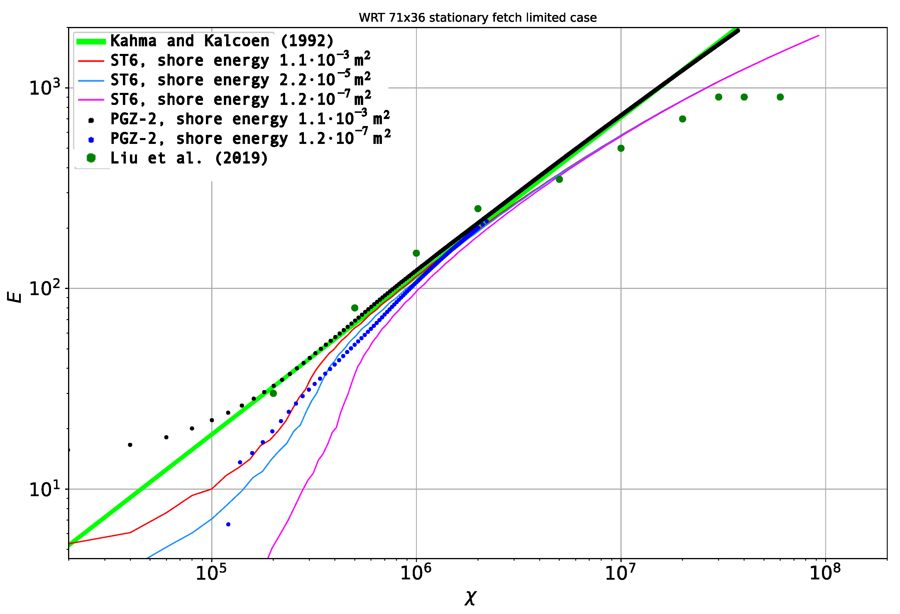
Figure 2 shows the total wave energy behavior dependence on the fetch for various models and field experimental observations as well as different values of the total energy on the shoreline.

One can see that, for the ST6 model described by Equation (2), the curve corresponding to the shore total energy value $1.1·{10}^{-3}$ m² is in a good agreement with the target dependence KC1992 for the 5–40 km fetch span as well as the numerical results of [15]. The situation is different, however, for other curves corresponding to lower shore total wave energy levels $2.2·{10}^{-5}$ m² and $1.2·{10}^{-7}$ m², which exhibit noticeable deviation from the KC1992 target dependence. Additionally, in the simplified model Equation (2), we were not able to reach the “steady sea state” observed in the numerical experiments by [15] for the 200–600 km fetch range. One more difference (idealization) with WW3 and other wave models is disactivating the linear input term, which is important at the initial stage of wave development. The effect of this is seen as a difference between PGZ-2 and other models for short dimensionless fetches. We plan to perform more detailed tuning of parts of our model to minimize the effect of numerical problems [37].

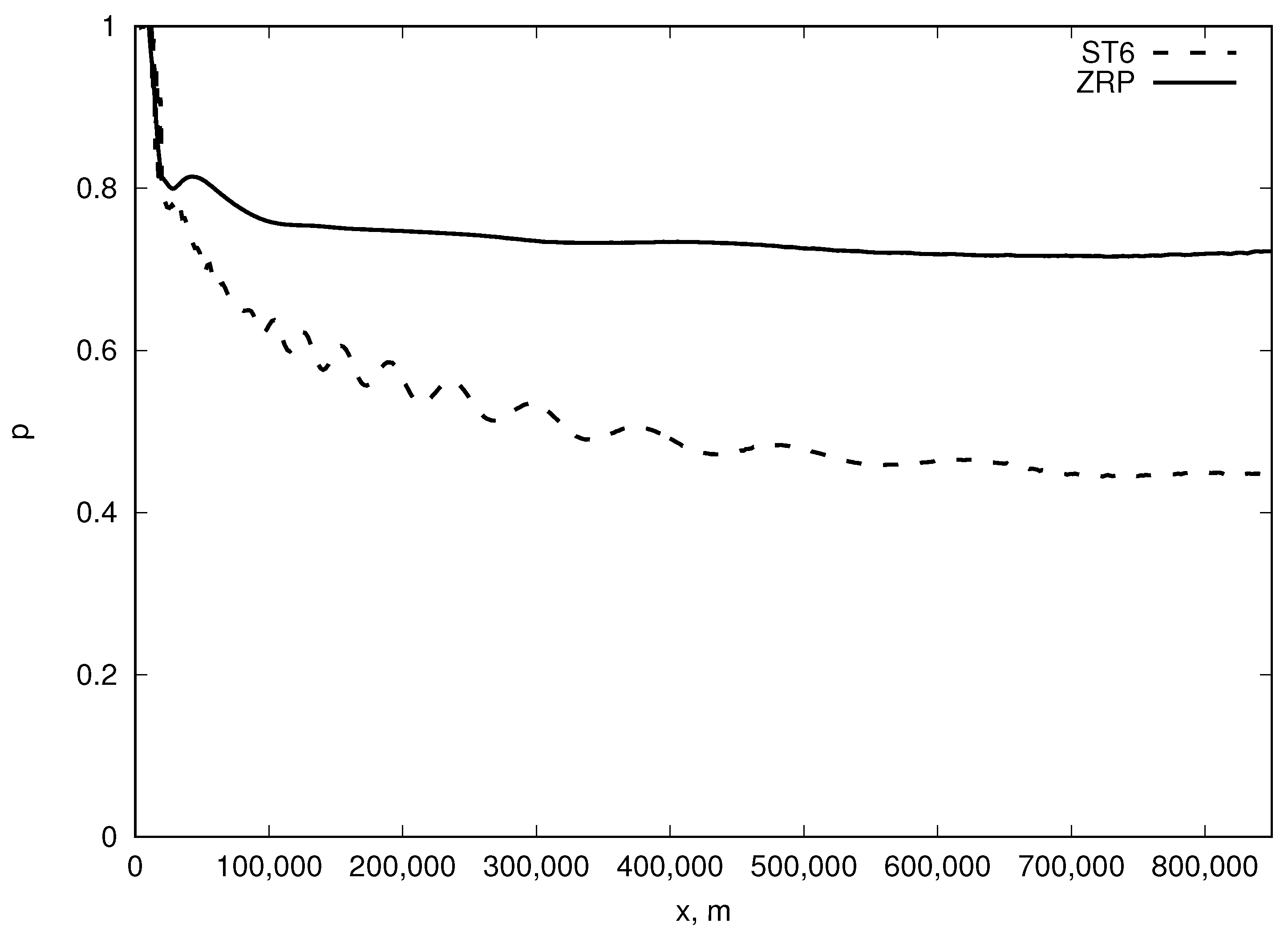
Figure 3 shows the local index p of power-like total wave energy dependence, derived from the data, plotted on Figure 2. It shows that the value of p in the ST6 case, described by Equation (2), asymptotically converges to $0.45$ with fetch growth independently on the total wave energy value at the shoreline.

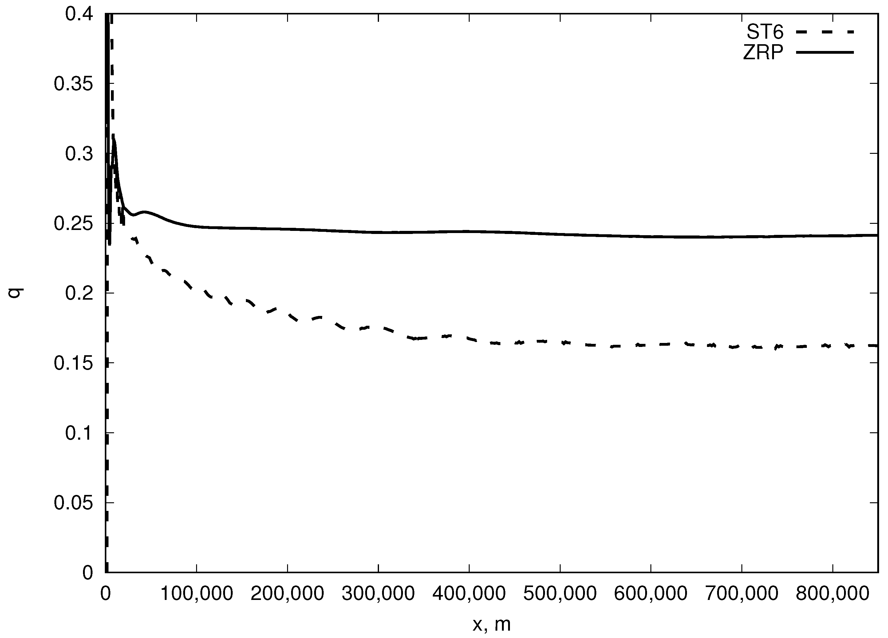
Similarly, Figure 4 plots the local index q of power-like mean frequency dependence in the ST6 case, described by Equation (2), converging asymptotically to $0.16$.

Figure 5 shows the combination $10q-2p$ for the same case, asymptotically converging to $0.72$. The observed value of this combination is not equal to 1 as it is supposed to be in Equation (5), and we are observing, therefore, the above-mentioned partial (i.e., related to portion of the fetch) quasi-self-similarity case for the ST6 model described by Equation (2).

Figure 6 shows 3D wave energy spectrum for the fetch $x=21$ km as the function of frequency f and angle $\theta$, localized in the angular spread of $\simeq {60}^{\circ }$ around the spectral maximum frequency for the ST6 case described by Equation (2).

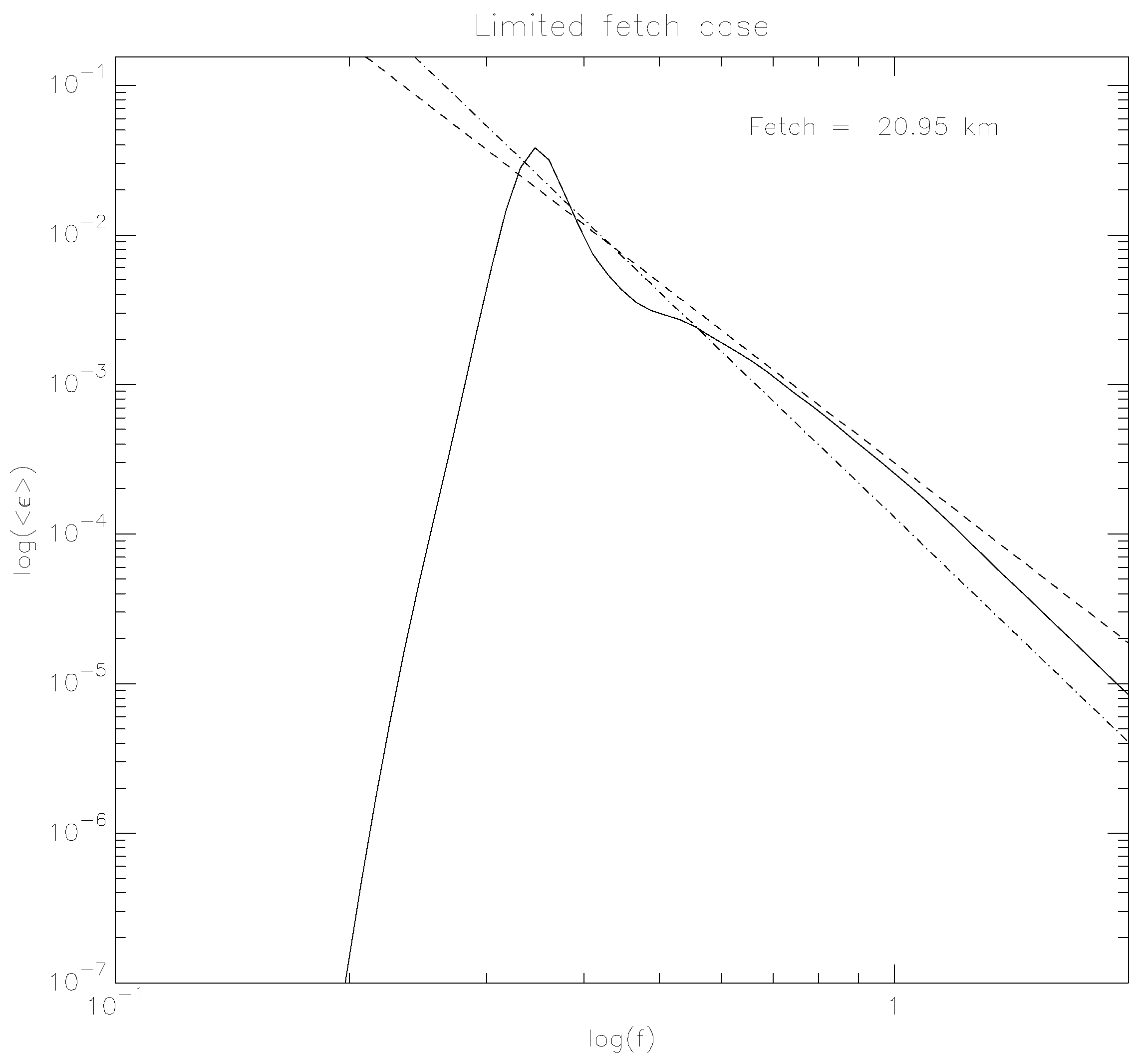
Figure 7 shows the angle-averaged wave energy spectrum corresponding to the previous figure as the function of the logarithm of frequency.

One can see the area of the spectral maximum, Kolmogorov–Zakharov (KZ) spectrum $\sim {\omega }^{-4}$ [34], and Phillips dissipation area $\sim {\omega }^{-5}$. These observations confirm the already known properties of surface wave turbulence observed in many field observations as well as numerical simulations before.

The general spectra structure, as obtained in numeric experiments, is the following. The pumping at some intermediate frequency results in the initial growth of energy spectrum there. This growth is bounded by the nonlinear interactions. Those nonlinear interactions result in the formation of the Kolmogorov spectrum which provides for the energy flow into the high frequencies by the cascade transfer of energy. The high frequency part of the spectra stabilizes in this way while the lower frequency part of the spectra continues its evolution. The energy pumping into the higher frequency part of the spectra results in the formation of the inverse cascade (which is the cascade transmittion of the wave number into the lower frequency part of spectra). Some energy is also transferred there, but it is much slower than the energy transfer into the high frequency, and this transfer is negligible in the total balance of energy transfer. This general pattern is present in all numerically calculated spectra and is also found in experimental ones. The cascading energy transfer by Zakharov–Filonenko spectra is very stable with respect to any disturbances.

3. Results

3.1. Alternative PGZ-2 Model: Wind Energy Input and Wave Dissipation Source Functions

As was shown in the previous section, the ST6 model exhibits some asymptotic partial quasi-self-similar properties of total wave energy growth on the fetch despite dependence on the boundary condition wave energy level. We will show here that it is possible to develop an alternative model, improving the properties of the S T6 model.

Let us consider a ZRP-like [8] wind energy source term for arbitrary frequency power dependence ${\omega }^s$ with unknown index s and amplitude A:

$$\begin{array}{ccc}\hfill & & S_{\mathrm{in}}^{\mathrm{PGZ}-2}(\omega ,\theta )=\gamma (\omega ,\theta )·\epsilon (\omega ,\theta )\hfill \end{array}$$

(12)

$$\begin{array}{ccc}& & \gamma (\omega ,\theta )=\left\{\begin{array}{c}A\frac{{\rho }_{air}}{{\rho }_{water}}\omega {\left(\frac{\omega }{{\omega }_0}\right)}^{s}q\left(\theta \right)\mathrm{for}{f}_{min}\le f\le f_d,\omega =2\pi f\hfill \\ 0\mathrm{otherwise}\hfill \end{array}\right.\hfill \end{array}$$

(13)

$$\begin{array}{ccc}& & q\left(\theta \right)=\left\{\begin{array}{c}{cos}^2\theta \mathrm{for}-\pi /2\le \theta \le \pi /2\hfill \\ 0\mathrm{otherwise}\hfill \end{array}\right.\hfill \end{array}$$

(14)

$$\begin{array}{ccc}& & {\omega }_0=\frac{g}{U_{10}},\frac{{\rho }_{air}}{{\rho }_{water}}=1.3·{10}^{-3}\hfill \end{array}$$

(15)

Here, air density is ${\rho }_{air}$ and water density is ${\rho }_{water}$; the frequencies $f_{min}=0.1$ Hz and $f_d=1.1$ Hz.

The model includes the classic Phillips tail [35,38], which is considered to be the result of some kind of energy dissipation. The wave energy dissipation source function is defined in the “implicit” manner [7,8] through the replacement of the portion of the dynamic spectrum part for $f>f_d$ by the Phillips tail $\sim {\omega }^5$ for every advance in time. We used $f_d=1.1$ Hz as a basic starting dissipation frequency, estimated from [31]. The future version of the model may include a more elaborate calculation of this value, for example, as in [39]. Other suitable methods of getting the cutoff frequency are based on assuming the effects of nonlinear dissipation (see [37]).

The spectrum value at $f_d$ for the Phillips part of the spectrum is defined from the continuity condition with the dynamic part of the spectrum. Then, the nonlinear four-wave interaction is calculated over the whole spectrum, consisting of its dynamic and Phillips continuation parts at every advance in time.

One should emphasize that the PGZ-2 alternative model appears independently on the ST6 one, since it is constructed in the completely different way to match KC1992 dependence. It requires the tuning of the wind forcing amplitude A, the frequency index s, as well as the shore total energy level.

3.2. Alternative PGZ-2 Model: Tuning and Numerical Results

The numerical experiments were carried out using the following parameters:

• Fourier space domain $f_{low}<f<f_{high}$, resolved by 72 logarithmically positioned discrete frequencies with $f_{low}=0.1$ Hz and $f_{high}=2.0$ Hz;
• Angular domain $-\pi <\theta \le \pi$ with 36 discrete angular directions, given the wind angle ${\theta }_{wind}=0$;
• Wind velocity $U_{10}=10$ m/s at a 10 m height above the ocean surface

The values A and s can be found by tuning procedure to match the dimensionless total wave energy dependence KC1992. The wind forcing index value s for PGZ-2 can be estimated from the relations Equation (6) through the exclusion of q:

$$\begin{array}{c}\hfill s=\frac{8-4p}{2p+1}\end{array}$$

Taking p from Equation (11), we present the following quasi-self-similar parameter set:

$$\begin{array}{c}\hfill p=0.79,q=0.258,s=1.87,10q-2p=1\end{array}$$

(16)

Another parameter to be tuned is the wind forcing amplitude A, which is obtained via best matching of the total wave energy growth curve, obtained in numerical simulation.

It appears, however, that the best fit of the energy growth is obtained for

$$\begin{array}{c}\hfill A=0.0089,s=2.2\end{array}$$

(17)

The tuned value $s=2.2$ somewhat exceeds target KC1992 value $s=1.87$, by $17.6\%$. This is chosen for practical reasons to provide for the better matching for the whole span of the KC1992 curve, including those parts (closer to the beginning) where the self-similarity is not fully established yet. We assume that the self-similar relations are still approximately correct there.

Figure 2 presents PGZ-2 total energy growth curves corresponding to the parameters of Equation (17) with two different values of shore energy. One can see that the PGZ-2 model exhibits dependence on the shore total energy value as does the ST6 model, but the scatter is much more narrow. Additionally, the PGZ-2 model reproduces the reference curve KC1992 earlier than ST6, starting from the fetch value of $\simeq 1.5$ km.

Figure 3, Figure 4 and Figure 5 present the values of indices p, q, and their combination, $10q-2p$, for the PGZ-2 case. One can see from Equation (16) that their values are closer to self-similar ones than the partial quasi-self-similar values for the ST6 case.

Figure 8 shows 3D distribution of the wave energy spectrum for the fetch $x=21$ km as the function of frequency f and angle $\theta$, localized in the angular spread of $\simeq {60}^{\circ }$ around spectral maximum frequency. While it reproduces the ST6 model spectral maximum value and spectral maximum frequency (see Figure 6), the spectral dependence on the angle is different. The scatter in not much more narrow than with ST6, but the distribution is multimodal, exhibiting the waves in the direction quasi-orthogonal to the wind.

Figure 9 shows the angle-averaged wave energy spectrum corresponding to Figure 8 as the function of the decimal logarithm of the frequency. As for the ST6 case (see Figure 7), one can see the area of the spectral maximum, Kolmogorov–Zakharov spectrum $\sim {\omega }^{-4}$ [34], and Phillips dissipation area $\sim {\omega }^{-5}$, but the peak is somewhat sharper. One can also see the difference between the amplitude of the spectra.

4. Discussion

This is the first article about our new model. The PGZ-2 model described here is a new development. The current version should be considered as a preliminary one. We plan to perform the various checks of it and compare it to the existing models and experimental data.

The development and the augmentation of the model may be performed in some different ways. The most obvious one is the further tuning of the coefficients. Other tuning may be a detailed studying of the transition between the ${\omega }^4$ and ${\omega }^5$ high-frequency spectrum tail. The transition point is defined by the balance between the nonlinear transfer of energy and damping and theoretically may be calculated from this balance.

The fetch-based calculations may be improved by including some kind of the back-scattering, i.e., the waves traveling (and transferring energy) to the coast from the open sea. Additionally, some energy may be transferred by the waves traveling along the coast, which also require consideration.

We believe that the numerical experiments using our new algorithm may be performed to improve the PGZ-2 model and to better tune it to the actual ocean wave conditions. We plan to continue the work on the PGZ-2 model and use it both for the fetch-based and duration-based calculations.

We performed the assessment of the ST6 model of wind energy input and wave dissipation source functions through numerical simulation of a stationary version of the Hasselmann equation with an exact four-wave interaction nonlinear term in the truncated Fourier space.

It is shown that the ST6 model exhibits partial quasi-self-similar properties, reproducing the reference field experimental total wave energy behavior for the fetch span from $\simeq 5$ to $\simeq 50$ km. For smaller values of the fetch, the ST6 model exhibits deviations from the target total wave energy reference curve KC1992, depending on the boundary value of the wave energy on the shore line.

We were neither able to reach the “steady sea state” state with the help of the truncated model nor to see any physical reason for its existence.

We formulated the new model of the balanced wind energy input and dissipation source terms with two unknown tunable parameters, the amplitude and index of the power-like wind source term, and call it PGZ-2. Those unknown values are obtained with the help of matching the PGZ-2 numerical results with the field experimentally observed energy growth curve KC1992 and theoretically predicted PGZ-2 self-similar relations.

The formulated PGZ-2 model significantly improves the correspondence of the total wave energy behavior for smaller fetches as well as larger ones with experimental curve KC1992.

Both ST6 and PGZ-2 models exhibit dependence of the wave energy growth along the fetch on the total wave energy value at the shore. The scatter of this dependence is lower for the PGZ-2 model.

One should note that the alternative PGZ-2 model should be construed as the demonstrational one and not for practical purposes since the KC1992 experiment analysis presents not quite typical behavior for the pool of the multiple experimental observations, studied in Badulin et al. [12], where the characteristic power-like total wave energy index value was $p=1$. In this relation, in the authors’ opinion, though close in spirit, the different ZRP approach to the formulation of the balanced source terms presents the better alternative.

The tuning of the PGZ-2 model was performed to be in agreement with the experimental data. More fine tuning may be performed on the basis of more numeric experiments.

We believe that the PGZ-2 model is a basis for further study. In the near future, we plan to study its properties in more detail and continue the tuning of the model.

References

- Hasselmann, K. On the non-linear energy transfer in a gravity-wave spectrum. Part 1. General theory. J. Fluid Mech. 1962, 12, 481–500. [Google Scholar] [CrossRef]
- Hasselmann, K. On the non-linear energy transfer in a gravity wave spectrum. Part 2. Conservation theorems; wave-particle analogy; irrevesibility. J. Fluid Mech. 1963, 15, 273–281. [Google Scholar] [CrossRef]
- Komen, G.J.; Cavaleri, L.; Donelan, M.; Hasselmann, K.; Hasselmann, S.; Janssen, P.A.E. Dynamics and Modeling of Ocean Waves; Cambridge University Press: Cambridge, MA, USA, 1994. [Google Scholar]
- The WAVEWATCH III Development Group (WW3DG). User Manual and System Documentation of WAVEWATCH III Version 6.07; Tech. Note 333; NOAA/NWS/NCEP/MMAB: College Park, MD, USA, 2019; 465p+Appendices. [Google Scholar]
- Young, I.R.; Banner, M.L.; Donelan, M.A.; McCormick, C.; Babanin, A.V.; Melville, W.K.; Veron, F. An Integrated System for the Study of Wind-Wave Source Terms in Finite-Depth Water. J. Atmos. Ocean. Technol. 2005, 22, 814–831. [Google Scholar] [CrossRef]
- Donelan, M.A.; Babanin, A.V.; Young, I.R.; Banner, M.L.; McCormick, C. Wave-Follower Field Measurements of the Wind-Input Spectral Function. Part I: Measurements and Calibrations. J. Atmos. Ocean. Technol. 2005, 22, 799–813. [Google Scholar] [CrossRef]
- Pushkarev, A.; Zakharov, V. Limited fetch revisited: Comparison of wind input terms, in surface wave modeling. Ocean Model. 2016, 103, 18–37. [Google Scholar] [CrossRef] [Green Version]
- Zakharov, V.; Resio, D.; Pushkarev, A. Balanced source terms for wave generation within the Hasselmann equation. Nonlinear Process. Geophys. 2017, 24, 581–597. [Google Scholar] [CrossRef] [Green Version]
- Zakharov, V.E. Theoretical interpretation of fetch limited wind-drivensea observations. Nonlinear Process. Geophys. 2005, 12, 1011–1020. [Google Scholar] [CrossRef]
- Badulin, S.I.; Pushkarev, A.N.; Resio, D.; Zakharov, V.E. Direct and inverse cascade of energy, momentum and wave action in wind-driven sea. In Proceedings of the 7th International Workshop on Wave Hindcasting and Forecasting, Banff, AB, Canada, 21–25 October 2002; pp. 92–103. [Google Scholar]
- Badulin, S.I.; Pushkarev, A.N.; Resio, D.; Zakharov, V.E. Self-similarity of wind-driven seas. Nonlinear Process. Geophys. 2005, 12, 891–946. [Google Scholar] [CrossRef] [Green Version]
- Badulin, S.I.; Babanin, A.V.; Zakharov, V.E.; Resio, D. Weakly turbulent laws of wind-wave growth. J. Fluid Mech. 2007, 591, 339–378. [Google Scholar] [CrossRef]
- Zakharov, V.E.; Badulin, S.I.; Geogjaev, V.V.; Pushkarev, A.N. Weak-Turbulent Theory of Wind-Driven Sea. Earth Space Sci. 2019, 6, 540–556. [Google Scholar] [CrossRef]
- Badulin, S.I.; Babanin, A.V.; Resio, D.; Zakharov, V. Numerical verification of weakly turbulent law of wind wave growth. In Proceedings of the IUTAM Symposium on Hamiltonian Dynamics, Vortex Structures, Turbulence; Springer: Berlin/Heidelberg, Germany, 2008; pp. 45–47. [Google Scholar]
- Liu, Q.; Rogers, W.E.; Babanin, A.V.; Young, I.R.; Romero, L.; Zieger, S.; Qiao, F.; Guan, C. Observation-Based Source Terms in the Third-Generation Wave Model WAVEWATCH III: Updates and Verification. J. Phys. Oceanogr. 2019, 49, 489–517. [Google Scholar] [CrossRef]
- Gagnaire-Renou, E.; Benoit, M.; Badulin, S.I. On weakly turbulent scaling of wind sea in simulations of fetch-limited growth. J. Fluid Mech. 2011, 669, 178–213. [Google Scholar] [CrossRef]
- Annenkov, S.Y.; Shrira, V.I. Effects of finite non-Gaussianity on evolution of a random wind wave field. Phys. Rev. E 2022, 106, L042102. [Google Scholar] [CrossRef] [PubMed]
- Alves, J.H.G.M.; Banner, M.L. Performance of a saturation-based dissipation-rate source term in modelling the fetch-limited evolution of wind waves. J. Phys. Oceanogr. 2003, 33, 1274–1298. [Google Scholar] [CrossRef]
- Tracy, B.; Resio, D. Theory and Calculation of the Nonlinear Energy Transfer between Sea Waves in Deep Water; WES Report 11; U.S. Army Engineer Waterways Experiment Station: Vicksburg, MS, USA, 1982. [Google Scholar]
- Webb, D.J. Non-linear transfers between sea waves. Deep-Sea Res. 1978, 25, 279–298. [Google Scholar] [CrossRef]
- Pushkarev, A. Comparison of different models for wave generation of the Hasselmann equation. Procedia IUTAM 2018, 26, 132–144. [Google Scholar] [CrossRef]
- Pushkarev, A.N.; Zakharov, V.E. Nonlinear amplification of ocean waves in straits. Theor. Math. Phys. 2020, 203, 535–546. [Google Scholar] [CrossRef]
- Pushkarev, A. Laser-like wave amplification in straits. Ocean Dyn. 2021, 71, 195–215. [Google Scholar] [CrossRef]
- Gagnaire-Renou, E. Amelioration de la Modelisation Spectrale des Etats de mer par un Calcul Quasi-Exact des Interactions Non-Lineaires Vague-Vague. Thèse pour L’obtention du Grade de Docteur, Université du Sud Toulon Var, Ecole Doctorale Sciences Fondamentales et Appliquées. 2009. Available online: https://theses.hal.science/tel-00595353/document (accessed on 24 February 2023).
- Hwang, P.; Wang, D.; Rogers, W.; Swift, R.; Yungel, J.; Krabill, A. Bimodal directional propagation of wind-generated ocean surface waves. arXiv 2001, arXiv:1906.07984. [Google Scholar] [CrossRef]
- Hwang, P.A.; Wang, D.W.; Yungel, J.; Swift, R.N.; Krabill, W.B. Do wind-generated waves under steady forcing propagate primarily in the downwind direction? arXiv 2019, arXiv:1907.01532v1. [Google Scholar]
- Hwang, P. Retondo080102Bimodal. 2002, Web Publication. Available online: https://www.researchgate.net/profile/Paul-Hwang-2/publication/275041443_Retondo080102Bimodal/links/55311a320cf20ea0a070df83/Retondo080102Bimodal.pdf (accessed on 24 February 2023).
- Hwang, P.A.; Wang, D.W.; Rogers, W.E.; Kaihatu, J.M. A Discussion on the Directional Distribution of Wind-Generated Ocean Waves. In Proceedings of the 6th International Workshop on Wave Hindcasting and Forecasting, Monterey, CA, USA, 6–10 November 2000; Resio, D.T., Ed.; Meteorological Service of Canada Environment Canada, Enviroment Canada: North York, ON, Canada, 2000; pp. 273–279. [Google Scholar]
- Simanesew, A.W.; Krogstad, H.E.; Trulsen, K.; Nieto Borge, J.C. Bimodality of Directional Distributions in Ocean Wave Spectra: A Comparison of Data-Adaptive Estimation Techniques. J. Atmos. Ocean. Technol. 2018, 35, 365–384. [Google Scholar] [CrossRef]
- Cavaleri, L.; Abdalla, S.; Benetazzo, A.; Bertottia, L.; Bidlot, J.R.; Breivik, O.; Carniela, S.; Jensen, R.E.; Portilla-Yandune, J.; Rogers, W.E.; et al. Wave modelling in coastal and inner seas. Prog. Oceanogr. 2018, 167, 164–233. [Google Scholar] [CrossRef]
- Long, C.; Resio, D. Wind wave spectral observations in Currituck Sound, North Carolina. JGR 2007, 112, C05001. [Google Scholar] [CrossRef] [Green Version]
- Zakharov, V.E.; Resio, D.; Pushkarev, A. New wind input term consistent with experimental, theoretical and numerical considerations. arXiv 2012, arXiv:1212.1069. [Google Scholar]
- Hasselmann, S.; Hasselmann, K.; Allender, J.H.; Barnett, T.P. Computations and Parameterizations of the Nonlinear Energy Transfer in a Gravity-Wave Specturm. Part II: Parameterizations of the Nonlinear Energy Transfer for Application in Wave Models. J. Phys. Oceanogr. 1985, 15, 1378–1391. [Google Scholar] [CrossRef]
- Zakharov, V.E.; Filonenko, N.N. The energy spectrum for stochastic oscillations of a fluid surface. Sov. Phys. Docl. 1967, 11, 881–884. [Google Scholar]
- Phillips, O. Spectral and statistical properties of the equilibrium range in wind-generated gravity waves. J. Fluid Mech. 1985, 156, 505–531. [Google Scholar] [CrossRef]
- Kahma, K.K.; Calkoen, C.J. Reconciling Discrepancies in the Observed Growth of Wind-generated Waves. J. Phys. Oceanogr. 1992, 22, 1389–1405. [Google Scholar] [CrossRef]
- Badulin, S.; Zakharov, V. The Phillips spectrum and a model of wind-wave dissipation. Theor. Math. Phys. 2020, 202, 353–363. [Google Scholar] [CrossRef] [Green Version]
- Phillips, O.M. The Dynamics of the Upper Ocean; Cambrige University Press: Cambrige, MA, USA, 1966. [Google Scholar]
- Lenain, L.; Pizzo, N. The contribution of high-frequency wind-generated surface waves to the Stokes drift. J. Phys. Oceanogr. 2020, 50, 3455–3465. [Google Scholar] [CrossRef]
Figure 1.
Limited fetch problem geometry. Constant wind of 10 m/s is blowing orthogonally to the fetch.
Figure 2.
The dimensionless total wave energy as the function of the dimensionless fetch (logarithmic coordinates). The curve notations are on the chart. ST6 and PGZ-2 data calculated by the authors, Kahma and Kalcoen from [36], Liu et al from [15].
Figure 3.
Total wave energy power-like local index p as the function of the dimensionless fetch.
Figure 4.
Frequency power-like local index q as the function of the dimensionless fetch.
Figure 5.
Magic number as the function of the dimensionless fetch.
Figure 6.
Spectral wave energy density as the function of the frequency and angle for ST6 case.
Figure 7.
Decimal logarithm of the angle averaged wave energy spectral density as the function of the decimal logarithm of frequency f for ST6 case. Dashed line—the KZ spectral fit ; dashed/dotted line—the Phillips spectral fit .
Figure 8.
Spectral wave energy density as the function of the frequency and angle for PGZ-2 case.
Figure 9.
Decimal logarithm of the angle-averaged wave energy spectral density as the function of the decimal logarithm of frequency f for PGZ-2 case. Dashed line—the KZ spectral fit ; dashed/dotted line—the Phillips spectral fit .
Disclaimer/Publisher’s Note: The statements, opinions and data contained in all publications are solely those of the individual author(s) and contributor(s) and not of MDPI and/or the editor(s). MDPI and/or the editor(s) disclaim responsibility for any injury to people or property resulting from any ideas, methods, instructions or products referred to in the content. |
© 2023 by the authors. Licensee MDPI, Basel, Switzerland. This article is an open access article distributed under the terms and conditions of the Creative Commons Attribution (CC BY) license (https://creativecommons.org/licenses/by/4.0/).
Share and Cite
MDPI and ACS Style
Pushkarev, A.; Geogjaev, V.; Zakharov, V. On ST6 Source Terms Model Assessment and Alternative. Water 2023, 15, 1521. https://doi.org/10.3390/w15081521
AMA Style
Pushkarev A, Geogjaev V, Zakharov V. On ST6 Source Terms Model Assessment and Alternative. Water. 2023; 15(8):1521. https://doi.org/10.3390/w15081521
Chicago/Turabian StylePushkarev, Andrei, Vladimir Geogjaev, and Vladimir Zakharov. 2023. "On ST6 Source Terms Model Assessment and Alternative" Water 15, no. 8: 1521. https://doi.org/10.3390/w15081521
Note that from the first issue of 2016, this journal uses article numbers instead of page numbers. See further details here.