Mapping Specific Constituents of an Ochre-Coloured Watercourse Based on In Situ and Airborne Hyperspectral Remote Sensing Data

Abstract

It is a well-known fact that water bodies are crucial for human life, ecosystems and biodiversity. Therefore, they are subject to regulatory monitoring in terms of water quality. However, land-use intensification, such as open-cast mining activities, can have a direct impact on water quality. Unfortunately, in situ measurements of water quality parameters are spatially limited, costly and time-consuming, which is why we proposed a combination of hyperspectral data, in situ data and simple regression models in this study to estimate and thus monitor various water quality parameters. We focused on the variables of total iron, ferrous iron, ferric iron, sulphate and chlorophyll-a. Unlike other studies, we used a combination of airborne hyperspectral and RGB data to ensure a very high spatial resolution of the data. To investigate the potential of our approach, we conducted simultaneous in situ measurements and airborne hyperspectral/RGB aircraft campaigns at different sites of the Spree River in Germany to monitor the impact of pyrite weathering on water bodies after open-cast mining activities. Appropriate regression models were developed to estimate the five variables mentioned above. The model with the best performance for each variable gave a coefficient of determination R² of 64% to 79%. This clearly shows the potential of airborne hyperspectral/RGB data for water quality monitoring. In further investigations, we focused on the use of machine learning techniques, as well as transferability to other water bodies. The approach presented here has great potential for the development of a monitoring method for the continuous monitoring of still waters and large watercourses, especially given the freely available space-based hyperspectral missions via EnMAP.

1. Introduction

The abundance, distribution and use of water are becoming ever more critical on a global scale [1]. Nevertheless, water is a decisive factor in the evolution, distribution and maintenance of ecosystems and biodiversity. Severe anthropogenic influences (e.g., eutrophication, extraction, contamination, sewage, toxins, coal mines and climate change) have already led to a partially irreversible deterioration and disturbance of freshwater ecosystems, their associated biodiversity and their loss of ecosystem services.

Lignite and coal are important energy sources in many countries. However, mining directly and indirectly affects surrounding ecosystems and nearby water bodies [2]. Before contaminated water is discharged into local surface waters, it is often collected in sedimentation ponds and treated with lime [3]. The liming process generates copious amounts of chemically stable sludge, which contains heavy metals. Furthermore, the groundwater level is also lowered during open-cast mining activities. In areas with soils containing iron disulphide minerals, e.g., marcasite or pyrite, low groundwater levels enable the reaction between these minerals, atmospheric oxygen and precipitation water, which leads to the decomposition of the minerals into sulphate, ferrous iron (Fe(II)) ions and hydrogen [4,5]. The low groundwater level also has a negative impact on the surrounding flora and fauna, as well as stream biodiversity [6,7,8,9]. When the open-cast mining activities are over, renaturation occurs and the groundwater rises naturally. Through this process, the products of pyrite weathering reach the local surface waters through aquifers [6]. In the oxygen-rich surface waters, the Fe(II) ions oxidise to ferrous iron (Fe(III)) ions and flocculate, leading to an ochre-like colouring of the water, which is consequently called ochre-coloured water. The ochre causes high turbidity in the water, and the deposition of iron precipitates, thus attenuating the living conditions for sediment dwellers. As a result, biodiversity in the affected areas decreases [10].

Monitoring of the effects of open-cast mining and subsequent renaturation using in situ measurement methods has been carried out for some time now. However, extensive temporal and spatial studies are time- and cost-intensive [11]. Airborne and spaceborne multispectral [12] and hyperspectral remote sensing (RS) [13] provide an alternative approach for monitoring various water quality indicators [14,15]. RS approaches provide continuous spatial and temporal maps of specific water quality parameters. Furthermore, they enable efficient, repeatable and standardised monitoring of a specific area and the identification and quantification of water constituents [12,16].

Owing to technical and methodological developments, hyperspectral RS is being increasingly used to derive water quality parameters, such as chlorophyll a (Chl-a) content [17], turbidity and visibility [18], depth [19] or coloured dissolved organic matter (CDOM) [17]. The quality of RS approaches and algorithms was greatly improved by the use of in situ monitoring data for calibration and validation. The use of hyperspectral RS approaches to detect water characteristics will play a crucial role in the regional and global monitoring of water quality indicators in the context of existing and future hyperspectral satellite missions, such as the DLR Earth Sensing Imaging Spectrometer (DESIS) [20], the Environmental Mapping and Analysis Program (EnMAP) [21], the PRecursore IperSpettrale della Missione Applicativa (PRISMA) [22] or the Hyperspectral Imager Suite (HISUI [23]).

Knowledge of the traits of water and its dissolved and particulate components forms the basis for numerous RS algorithms [24,25]. Consequently, all optically active water constituents determine the reflectance (RRS) of the water through the specific absorption and backscattering behaviour per wavelength [26]. On the other hand, the RS of water constituents often relies on empirical models [16,25,27]. These models try to establish statistical relationships between remote sensing signals and in situ data from locally collected water samples. In empirical models, mechanistic explanations based on the radiative transfer equation are considered from statistical correlations. For waterbodies with similar optical properties, empirical models based on a limited amount of local field data may provide fast and accurate results with a high spatial resolution for a specific aquatic environment [28].

The relevant spectral range to derive optically active water constituents, i.e., CDOM, phytoplankton and total suspended matter (TSM) [25,29], ranges between 400 and 1000 nm. Water absorbs a large amount of sunlight and exhibits low backscattering behaviour, which only increases within the wavelength range of 400 to 500 nm [30]. CDOM mainly absorbs light within the wavelength range of 400 and 500 nm [31,32]. Therefore, most CDOM-derivation models are based on this wavelength range [33]. Humic substances and other dissolved organic carbon (DOC) are often assigned to this group. Phytoplankton is one of the living and particulate components of waters measured using RS and Chl-a, which is a key molecule of photosynthetically active organisms that is often used as an indicator of biomass production. The spectral characteristics of Chl-a include the low reflectance between 400 and 500 nm [32] and maximum reflectance at 580 nm [27,30]. The non-living particulate matter can be assigned to TSM. This group includes particulate organic deceased matter or small sand particles [30]. Water bodies with a high TSM concentration exhibit increased backscattering behaviour. In addition to the abovementioned active water constituents, TFe, Fe(II), Fe(III) and sulphate also affect the water colouring.

Repic et al. [34] already used multispectral video data with three spectral channels in the wavelength range from 400 to 1500 nm to detect the iron ions of two abandoned open pit lakes. Furthermore, Anderson and Robbins [35] developed a method to spectrally discriminate acid mine drainage (AMD) and natural streams using water samples, in situ spectral data and multispectral RS data. They found that a pH < 4 may have prevented the oxidation of Fe(II) to Fe(III). As a result, iron could not precipitate in the form of Fe(III). On this basis, Anderson and Robbins [35] found wavelengths at 650 nm and 750 nm to be very sensitive to iron oxides. Williams et al. [36] used the same airborne multispectral video system to identify and map AMDs. At a pH of 3.2 and 6.9, they were able to show that the 650 and 750 nm wavelengths were sensitive enough to visualize the ochre precipitates of the mine water.

Following the initial studies on AMDs, in subsequent years, research focused on open-cast mining residual lakes [30,37,38].

In recent decades, significant progress was achieved in monitoring and assessing the quality of inland waters using RS [12,15,25]. Through improved computer-based interpretation techniques and spectrally (up to 3.25 nm per channel) plus spatially (up to 50 cm ground sampling distance) high-resolution satellites, coastal zones and lakes were increasingly monitored [39,40,41]. Owing to their small spatial extent and complex chemical composition, small watercourses have received relatively little attention [42] and the focus of previous analyses was on very wide rivers, such as the Mississippi, the Gironde or the Rhein, and river estuaries [13,43,44,45,46].

By using the institute’s own gyrocopter with extensive sensor technology (hyperspectral/RGB/TIR), Fe(II) and Fe(III) were thus recorded, modelled and derived separately for the first time with low spatial RS data resolution (50 cm), even with lower concentrations of iron for smaller flowing watercourses with a neutral pH.

The objectives of this study were as follows:

• To show that airborne hyperspectral/RGB RS technologies are suitable for monitoring water quality parameters for small streams.
• To propose simple linear modelling approaches for modelling and predicting TFe, Fe (II), Fe(III), sulphates and Chl-a in ochre streams.
• To develop and test a robust procedure to derive TFe, Fe(II), Fe(III), sulphates and Chl-a based on airborne hyperspectral RS data and simultaneous field sampling in a river section influenced by mining activities.
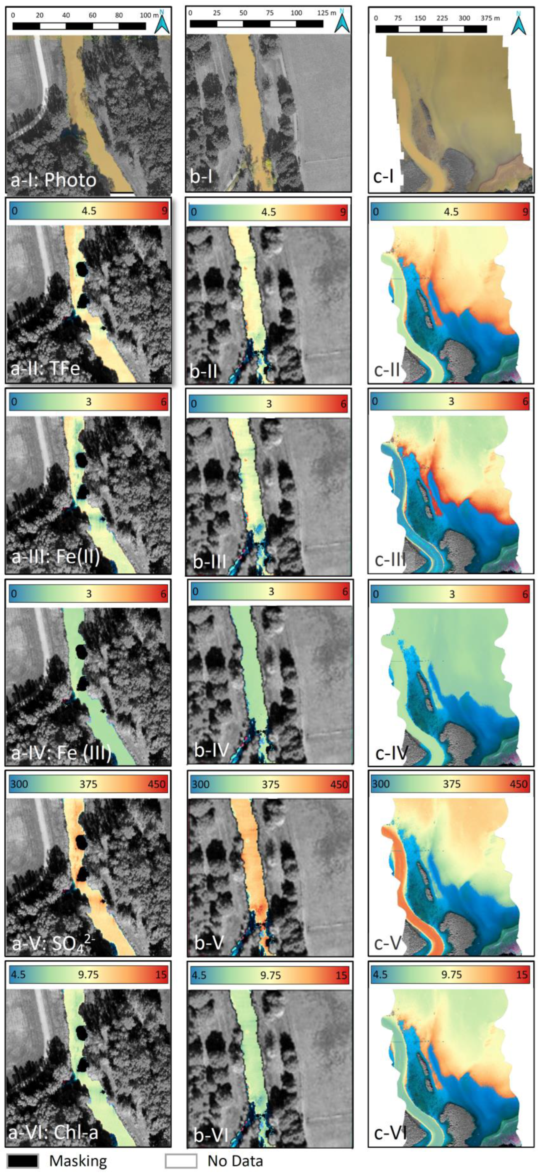
• To transfer the point results from the in situ field sampling to the area.
• To discuss the framework conditions as well as the limitations of the presented approach.

2. Materials and Methods

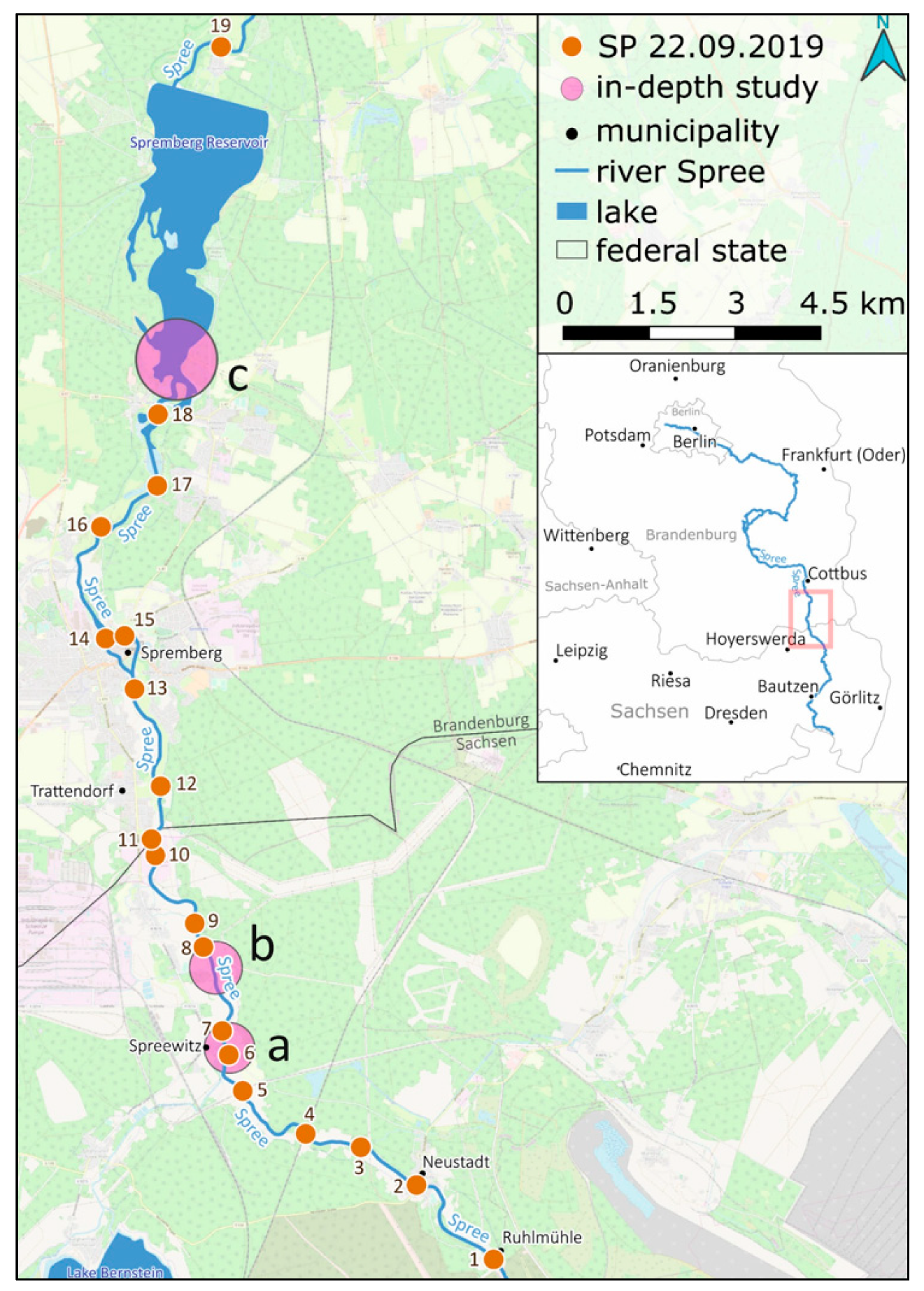
2.1. Study Area

The study area was located southeast of Berlin in Lusatia along the River Spree and extended from the village Ruhlmühle to the end of the Spremberg reservoir (Figure 1). The flow direction of the Spree was from south to north.

Open-cast lignite mining in Lusatia has the greatest impact on this section of the river [47]. Increased loads from the products of pyrite weathering into the Spree River caused (1) an increased concentration of sulphate, (2) an increased concentration of Fe(II) and Fe(III), and (3) increased turbidity of the water body owing to sludge formation.

In the mid-20th century, the groundwater level in the study area was lowered significantly due to open-cast mining. Consequently, the pyrite in the soil reacted with oxygen in the air and precipitation water (Figure 1) and subsequently disintegrated into Fe(II), sulphate and hydrogen ions. Following the implementation of recovery measures in 1990, many open-cast mines were closed and flooded via the natural process. Thus, the groundwater level rose in many parts of the mining area [48]. The products of pyrite weathering in the hydrosphere reached surrounding surface waters via aquifers. The Fe(II) ions were oxidized in the oxygen-rich water to Fe(III) ions [5].

In pH-neutral water bodies, Fe(III) ions were hydrolyzed to ferrous-oxyhydroxide (Fe(III)-oxyhydroxide) and flocculated [5,49]. A Fe(III)-hydroxide concentration of 2 mg/L causes the water to appear yellow-to-reddish-brown in colour [50,51]. The process of iron clogging is schematically summarized in Figure 2.

The municipalities of Ruhlmühle and Spreewitz, the mouth of the industrial canal of Schwarze Pumpe industrial park, the pre-dam Bühlow and the Spremberg reservoir were significant spots in the study area (Figure 1). Analyses conducted by Bilek and Koch [6] showed the discharge of Fe(II) loads from anoxic groundwater into the oxygen-rich river water. Uhlmann et al. [52] observed the input of large amounts of Fe(II) into the river at the village Ruhlmühle (SP 1 in (Figure 1). In the oxygen-rich water and under natural pH conditions, the Fe(II)-oxide flocculated out as Fe(III)-oxyhydroxide, causing an ochre colour in the river water.

At Spreewitz (SP 7 in Figure 1), the Kleine Spree River flows into the Spree River and is enriched with iron. In the south of Trattendorf town (SP 8 in Figure 1), the canal from the Schwarze Pumpe industrial park increases the sulphate concentration in the Spree River. The treatment of the water in a pre-dam of the Spremberg reservoir (Bühlow) is intended to increase iron retention [53] (SP 18 in Figure 1). In the Spremberg reservoir, the reduced flow velocity leads to the deposition of Fe(III)-oxyhydroxide, as well as reduced turbidity (between SP 18 and 19 in Figure 1). This process significantly reduces the brown colouring of the Spree below the Spremberg reservoir.

2.2. In Situ Data

On 22 September 2019, a field campaign was conducted to simultaneously collect RS data and field samples to develop empirical derivation models. Water samples were taken between 10 a.m. and 2 p.m. at the same time that a gyrocopter flew over (see Section 2.3) using a scoop down to a depth of 30 cm. Thus, every sample represented a composite sample of the top water column. The in situ data served as reference data for the development of additional empirical models in order to derive the distribution of water constituents over an extensive area from airborne hyperspectral data.

The total iron (TFe) was measured following digestion with 2 mL of H₂O₂ (5%) and 2 mL of H₂SO₄ (5 M) according to DIN 38406 using flame-atomic absorbance spectroscopy (AAS PinAAcle 900T, PerkinElmer, Waltham, MA, USA). The dissolved Fe(II) analysis was prepared on site according to DIN 38406 by stabilizing 15 mL of the filtrated water sample with 0.15 mL of 5 M sulphuric acid and storing it free of air bubbles. On the same day, the concentration of Fe(II) was determined photometrically after complexation with 1.10 phenanthroline (Spekol 1500, Analytik Jena, Jena, Germany). The total Fe(III) concentration was calculated using the difference between the TFe concentration and the Fe(II) concentration. Sulphate was determined according to DIN EN ISO 10304-1 by filtering the water sample on site. The sulphate concentration was quantified using ion chromatography (Compact IC Flex 930, Metrohm, Switzerland). To determine the dissolved substances, the sample was filtered using a syringe with a 0.45 µm filter (cellulose acetate; Whatman GmbH, Dassel, Germany). The unfiltered water samples for determining the Chl-a concentration were stored on site in 1 L vessels in a dark and cool place and processed further within 24 h. In the laboratory, the analysis was performed via HPLC (Waters Alliance, Milford, MA, USA) according to the procedure reported by Mehnert et al. [54]. The uncertainty of the analytical replicates in these analyses was typically <3%.

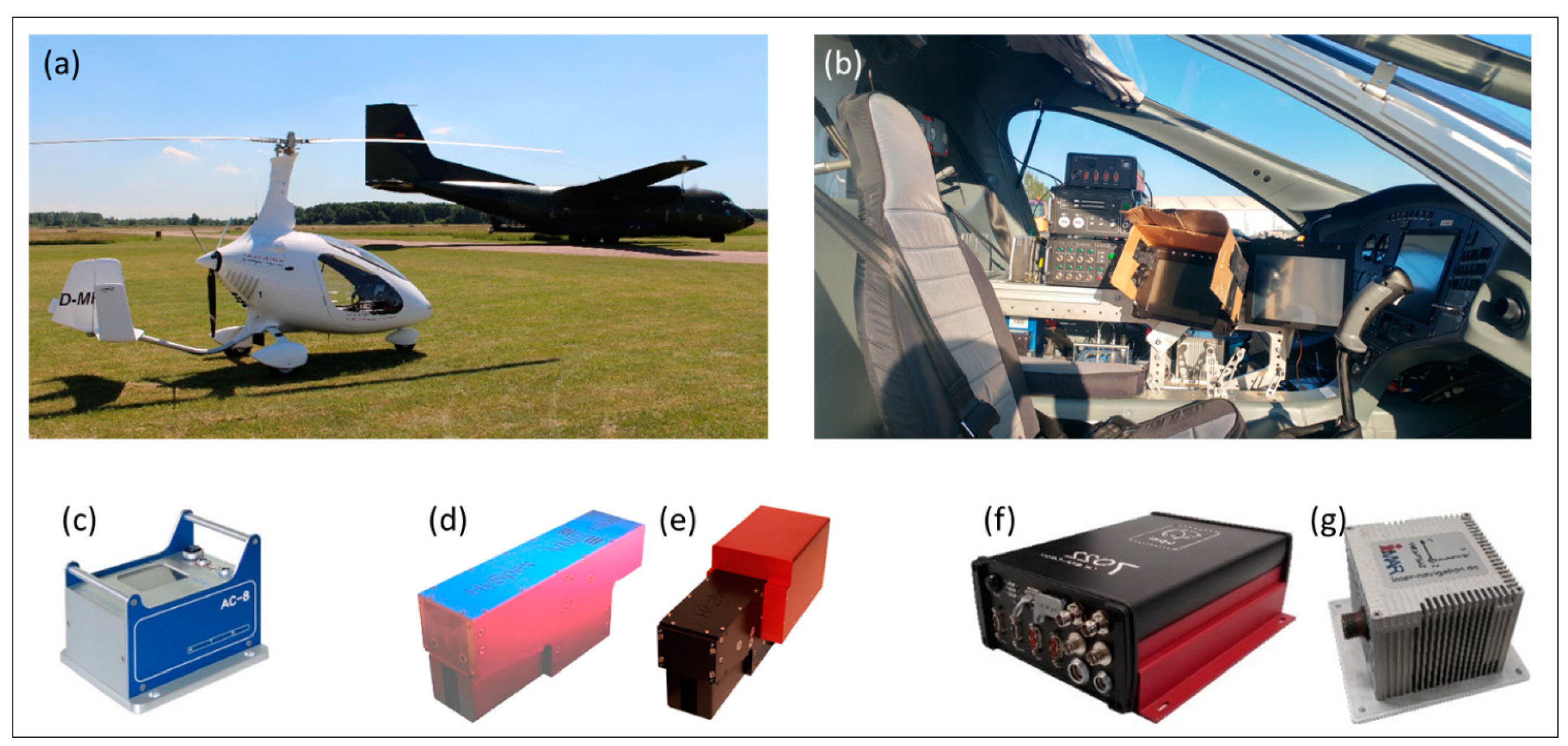
2.3. Remote Sensing Data

The gyrocopter at the Institute for Geoinformation and Surveying of the Anhalt University (see Figure 3) was used to record the hyperspectral RS data (HySpex VNIR, VSWIR) in the research area within the wavelength range of 400–2500 nm. The flight altitude was 600 m. Usually, hyperspectral data within the wavelength range of 400–1000 nm are used to derive water constituents. Because of the high turbidity and high TFe concentration throughout the study area, the wavelength range of 1000–2500 nm will be investigated further.

For the monitoring, the digital camera NIKON D800e (see Figure 3c) and the hyperspectral sensors HySpex VNIR 1600 (400–1000 nm) and HySpex SWIR 384 (1000–2500 nm) from Norsk Elektro Optikk AS (Neo) were used as optical sensors (see Figure 3d,e). An inertial navigation system (INS) was used for the high-precision acquisition of position and orientation data. The INS consisted of a GNSS receiver from PPM and an inertial measurement unit (IMU) from iMAR (see Figure 3f,g). The sensors are triggered automatically by the flight management software Aviatrix.

To detect small but significant spectral differences, the spectral sampling rate of the HySpex VNIR was set to a bandwidth of 7.4 nm. This resulted in 80 channels within the spectral wavelength range of 400–1000 nm. At an altitude of 600 m, the ground-sampling distance (GSD) was 20 cm. The data from the HySpex SWIR had a spectral sampling rate of 5.45 nm with 288 channels within the wavelength range of 1000–2500 nm. The GSD of the HySpex SWIR was 60 cm at a flight altitude of 600 m.

As a basis for processing the hyperspectral data, a near-true orthophoto with a GSD of 6 cm was calculated from the RGB images using the structure from motion (SfM) algorithm [55]. This served as the basis for determining the boresight angle for processing the hyperspectral data. These data were rectified, georeferenced and atmospherically corrected using PARGE Version 3.3 [56] and ATCOR-4 Version 7.2 [57] software. Owing to the flight altitude of 600 m and a field of view of the hyperspectral sensors of 34° and 32°, respectively, adjacent and atmospheric effects significantly influenced the hyperspectral images.

The atmospheric correction was carried out with the ATCOR software using an urban model based on the presence of open-cast mines, industry and urban areas. Specific absorptions and reflectances of the atmosphere influence a large part of the measurable radiance, which requires correction for reliable derivation [58]. For this reason, according to Ray [59], the determined pixel values represent an apparent reflectance (aRRS), which is comparable with the RRS in most cases.

Although aRRS is comparable to RRS, adjacent effects cannot be compensated for using an atmospheric correction because the information on the simultaneous illumination conditions is not available. To exclude these influences for subsequent calculations, the hyperspectral image data of the surrounding river environment were masked out, meaning that only the relevant spectral information of the river forms the basis of all subsequent model calculations. Adjacent effects can impair the measurable radiance through reflections and lead to saturation of the sensor [60]. The adjacent effects can be assigned, for example, to reflections of solar panels or waves from the water body or even shadows from vegetation on the water’s surface. If these influences could also be seen on the water’s surface, they were also masked.

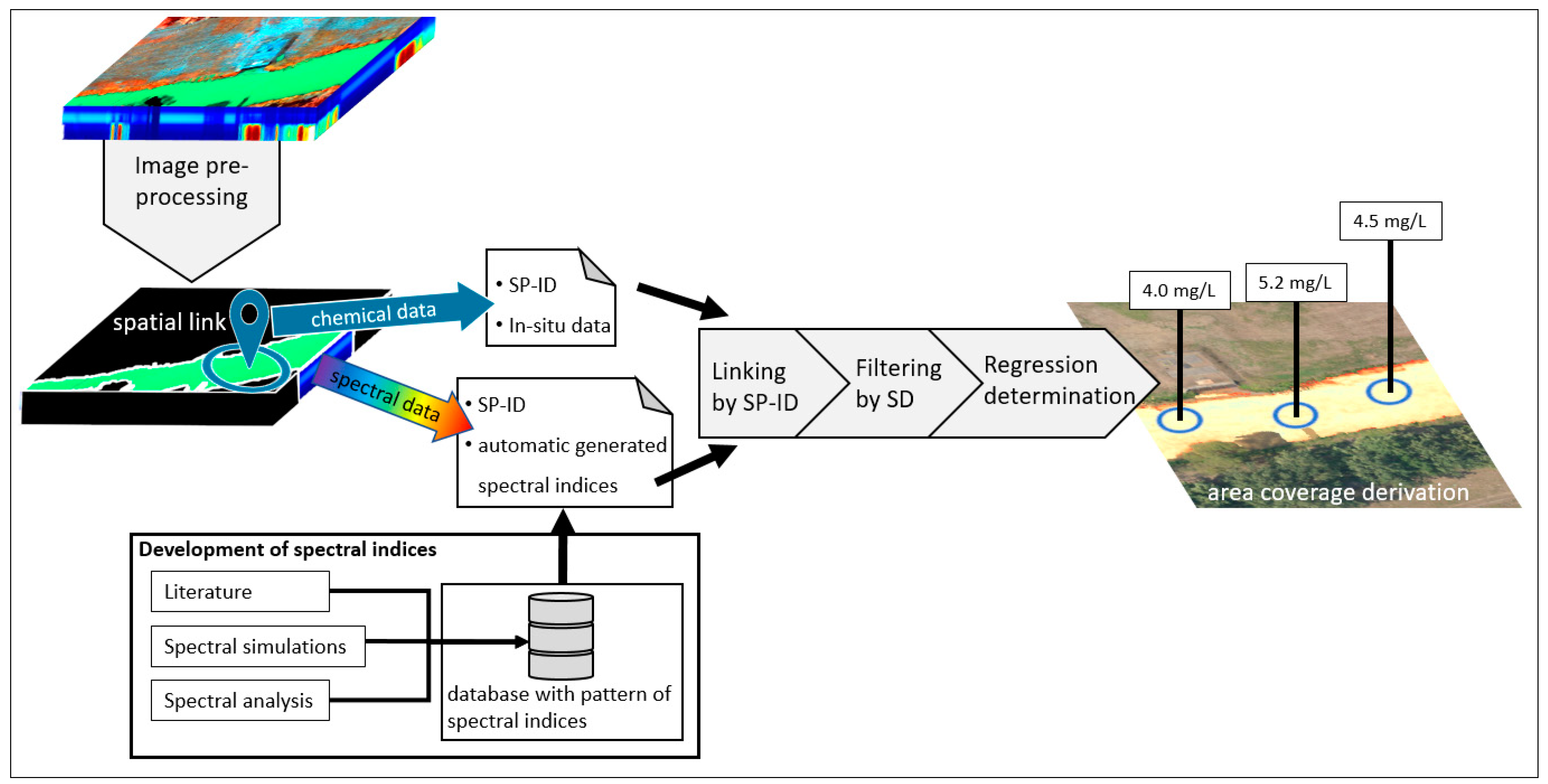
2.4. Model Development for the Area-Wide Derivation

The empirical approach links the in situ sampling points (SPs) and airborne hyperspectral RS data via regression to determine the coefficient of determination (R²) between them [26,61]. For the area coverage derivation of the water constituents, the workflow can be divided into six tasks: (1) image pre-processing, (2) data linking in two steps, (3) development of spectral indices, (4) data filtering using the standard deviation (SD), (5) regression determination and (6) derivation. Due to the two separate steps for linking the SP data with the RS data, an identification number (ID) was assigned to each SP (SP-ID) (see Figure 4).

Initially (task 1), the hyperspectral data was processed as described in Section 2.3. This was followed (task 2) by linking the in situ data with the hyperspectral data in two steps. First, the link was made through the GNSS position. This allowed for the extraction of specific spectral information for each sampling point and the assignment of the particular information to the sampling point identification number (SP-ID). Second, we linked the spectral indices based on specific wavelength bands with the in situ data. As described by Ulrich et al. [62] the spectral indices are based on previous studies on the determination of water quality [27,30,32,45,63,64,65,66], spectral simulations and analyses. Based on this, the following spectral indices were developed as a template (Equations (1)–(5); task 3):

Type 1 single Wavelength: SI 1 = R_RS(b1)

(1)

$$\mathrm{Type} 2 \mathrm{Ratio}: SI 2=\frac{R_{\mathrm{RS}}\left(\mathrm{b}1\right)-R_{\mathrm{RS}}\left(\mathrm{b}2\right)}{R_{\mathrm{RS}}\left(\mathrm{b}1\right)+R_{\mathrm{RS}}\left(\mathrm{b}2\right)}$$

(2)

$$\mathrm{Type} 3 \mathrm{Ratio}: SI 3=\frac{R_{\mathrm{RS}}\left(\mathrm{b}1\right)-R_{\mathrm{RS}}\left(\mathrm{b}3\right)}{R_{\mathrm{RS}}\left(\mathrm{b}2\right)-R_{\mathrm{RS}}\left(\mathrm{b}3\right)}\mathrm{t}$$

(3)

$$\mathrm{Type} 4 \mathrm{Ratio}: SI 4=\frac{R_{\mathrm{RS}}\left(\mathrm{b}1\right)-R_{\mathrm{RS}}\left(\mathrm{b}3\right)}{R_{\mathrm{RS}}\left(\mathrm{b}2\right)+R_{\mathrm{RS}}\left(\mathrm{b}3\right)}$$

(4)

$$\mathrm{Type} 5 \mathrm{Slope}: SI 5=\frac{R_{RS}\left(b2\right)-R_{RS}\left(b1\right)}{b2-b1}$$

(5)

where R_RS: reflectance and b: band of the hyperspectral image.

To improve the derivation accuracy, the water samples were filtered using 2.5 times the SD to eliminate incorrect samples or analyses (task 4).

Next (task 5), suitable regression models were determined for each water constituent: TFe, Fe(II), Fe(III) and sulphate. For this purpose, each chemical parameter was related to 100 spectral indices and tested for linear, logarithmic, exponential and potential regressions (Equations (6)–(9)) following the general regression model presented by the International Ocean-Colour Coordinating Group [67].

$$\mathrm{Linear} \mathrm{regression}: \widehat{p}=\alpha \times \left(SI\right)+\beta$$

(6)

$$\mathrm{Logarithmic} \mathrm{regression}: \widehat{p}=\alpha \times log\left(SI\right)+\beta$$

(7)

$$\mathrm{Exponential} \mathrm{regression}: \widehat{p}=\beta \times e^{\alpha *\left(SI\right)}$$

(8)

$$\mathrm{Potential} \mathrm{regression}: \widehat{p}=\beta \times {\left(SI\right)}^{\alpha }$$

(9)

where $\widehat{p}$: parameter to be estimated in the quantitative unit; $SI$: spectral index; R_i: spectral band; and α and β: regression parameters between the spectral and in situ data.

The most suitable type was determined using the coefficient of determination (R²) value and stored with the corresponding regression parameters. Consequently, this procedure resulted in a specific regression model for each water constituent per spectral index for the area coverage derivation.

Finally, for the accuracy analysis, the RMSE and relative RMSE (rRMSE) values were calculated for 10 derivation models with the highest R² (task 6). For this purpose, the derived concentrations at the sampling site were linked to the filtered limnic data. The rRMSE was calculated according to the procedure reported by Gao et al. [68] and Wang and Lu [69] (Equation (10)). This allowed for the most appropriate spectral index to be selected for each water body constituent.

$$rRMSE [\%]=\frac{RMSE}{\overline{Obs}}\times 100\%$$

(10)

where $\overline{Obs}$: mean value of the observations.

3. Results and Discussion

The limnological characteristics of watercourses influenced by mining differ from those of natural watercourses [37]. This is because of the geological conditions, the geohydrological processes of the mining areas and a rise in the groundwater level [38]. In this study, a framework consisting of simultaneous monitoring of in situ data and airborne hyperspectral/RGB data was presented, enabling the modelling of water quality indicators (TFe, Fe(II), Fe(III), sulphate and Chl-A).

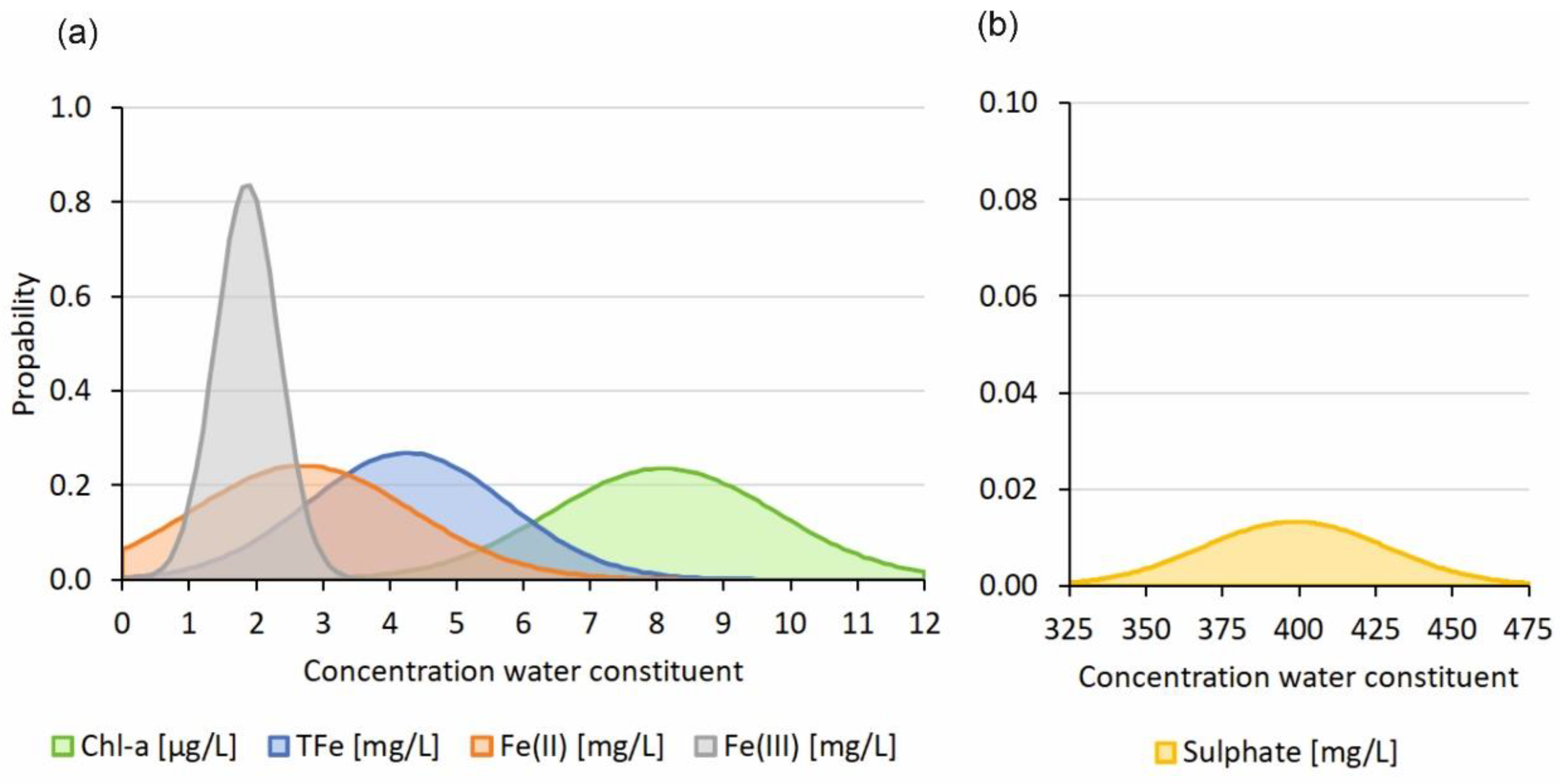
3.1. In Situ Measurements of Water Quality

In situ data from 19 sampling locations were analysed for TFe, Fe(II), Fe(III), sulphate and Chl-A (see

Table 1. List of the in situ monitored chemical parameters. The SP-IDs 3-14 and 16-18 were used for the derivation models. Thus, the total quantity (N) ranged between 13 and 15 values. This was due to suitable spatial overlaying with the RS data.

SP ID	TFe [mg/L] (1)	Fe(II) [mg/L]	Fe(III) [mg/L]	Sulphate [mg/L] (2)	Chl-a [µg/L]
1	0.7	0.04	0.66	356	11.9
2	2.8	2.19	0.61	362	12.31
3	3.8	2.45	1.35	364	9.76
4	5.7	4.53	1.17	369	10.64
5	6.3	4.47	1.83	367	9.96
6	6.3	5.17	1.13	366	11.04
7	7.0	5.28	1.72	336	10.20
8	4.9	3.1	1.8	436	7.41
9	4.7	2.74	1.96	434	7.06
10	3.9	2.00	1.9	422	6.92
11	3.9	1.89	2.01	420	7.18
12	4.00	1.52	2.48	421	7.03
13	3.2	0.94	2.26	421	6.63
14	2.3	0.58	1.72	426	6.15
15	3.1	0.64	2.46	419	6.32
16	3.2	0.31	2.89	398	8.66
17	1.8	<0.05	-	399	6.43
18	2.9	<0.05	-	399	6.35
19	0.6	<0.05	-	430	10.39
Mean	3.74	2.37	1.75	3.74	2.37
Standard deviation	1.74	1.68	0.62	31	2.05
Maximum	7.00	5.28	2.89	436	12.32
Minimum	0.60	0.04	0.61	336	6.15

Note: The regulatory limits according to German law are (https://www.gesetze-im-internet.de/trinkwv_2001/BJNR095910001.html, accessed on 4 December 2023): ⁽¹⁾ 0.2 mg/L for (total) iron and ⁽²⁾ 250 mg/L for sulphate.

). Only 15 of the sampling locations were covered by the gyrocopter survey and used to calibrate the remote sensing data. Table 1 gives an overview of the monitored limnic parameters and their mean values, standard deviations, minima and maxima.

Figure 5 shows the plot of the distribution of the recorded in situ water parameter measurements for Chl-a, TFe, Fe(II), Fe(III) (Figure 5a) and sulphate (Figure 5b) based on a probability function. The value range of the sulphate concentration deviated strongly from the concentrations of the other water constituents.

Likewise, the correlation matrix (

Table 2. Correlations matrix with the recorded in situ water parameters: TFe, Fe(II), Fe(III), sulphate and Chl-a.

	TFe [mg/L]	Fe(II) [mg/L]	Fe(III) [mg/L]	Sulphate [mg/L]	Chl-a [µg/L]
TFe [mg/L]	1.00	0.97	−0.50	−0.58	0.79
Fe(II) [mg/L]	0.97	1.00	−0.70	−0.70	0.79
Fe(III) [mg/L]	−0.50	−0.70	1.00	0.48	−0.56
Sulphate [mg/L]	−0.58	−0.70	0.48	1.00	−0.84
Chl-a [µg/L]	0.79	0.79	−0.56	−0.84	1.00

) shows that the in situ water parameters Chl-a, TFe, Fe(II), Fe(III) and sulphate were correlated with each other, making modelling and a clear delineation of the individual water parameters using hyperspectral data difficult. TFe and Fe(II) showed the highest correlations with r = 0.97. This indicates a high proportion of dissolved Fe(II) in the measured water depth of 30 cm. Furthermore, the water body might not have been completely saturated with oxygen on the day of the measurement. The correlation between Fe(III) and TFe was r = −0.50 and between Fe(III) and Fe(II) was r = −0.70. Both values indicated that the Fe(III) concentration increased or decreased inversely to the concentrations of TFe and Fe(II) (see Table 2).

Similarly, sulphate also showed a correlation of r = −0.58 with TFe and r =−0.70 with Fe(II). This was due to additional inputs of sulphate from the Schwarze Pumpe industrial park at sample point 8 (see Figure 1). Chl-a indicated a correlation of r = 0.79 with TFe and Fe(II). This indicated a uniform decrease of the Chl-a concentration in relation to the TFe and Fe(II) concentrations, resulting from the increasing ocherous colour due to the flocculation of the Fe(III) ions. Accordingly, the correlation between Chl-a and Fe(III) was r = −0.56. Moreover, Chl-a also showed a correlation of r = −0.84 with sulphate.

Figure 6 shows five spectra within the wavelength range of 415 to 1615 nm. The corresponding chemical parameters are listed in Table 1. These spectra were extracted from the hyperspectral images at sampling points 4, 7, 11, 16 and 19.

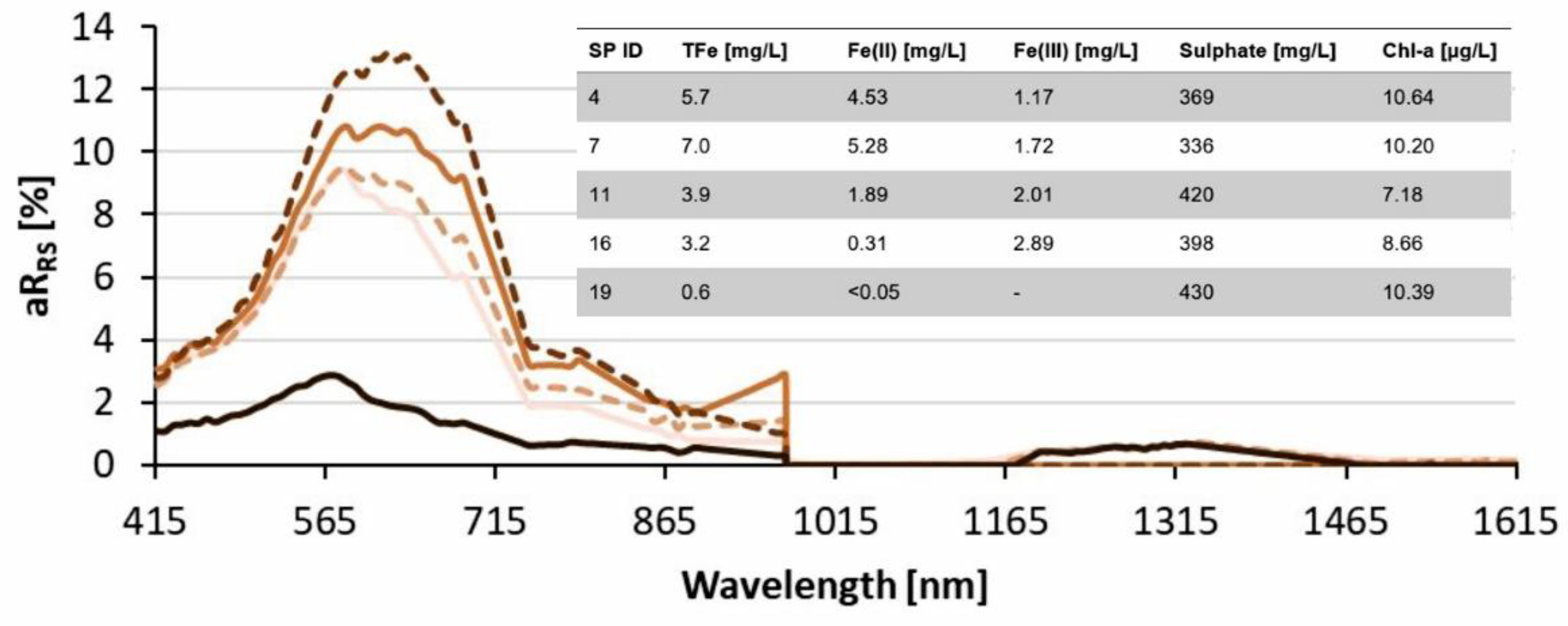
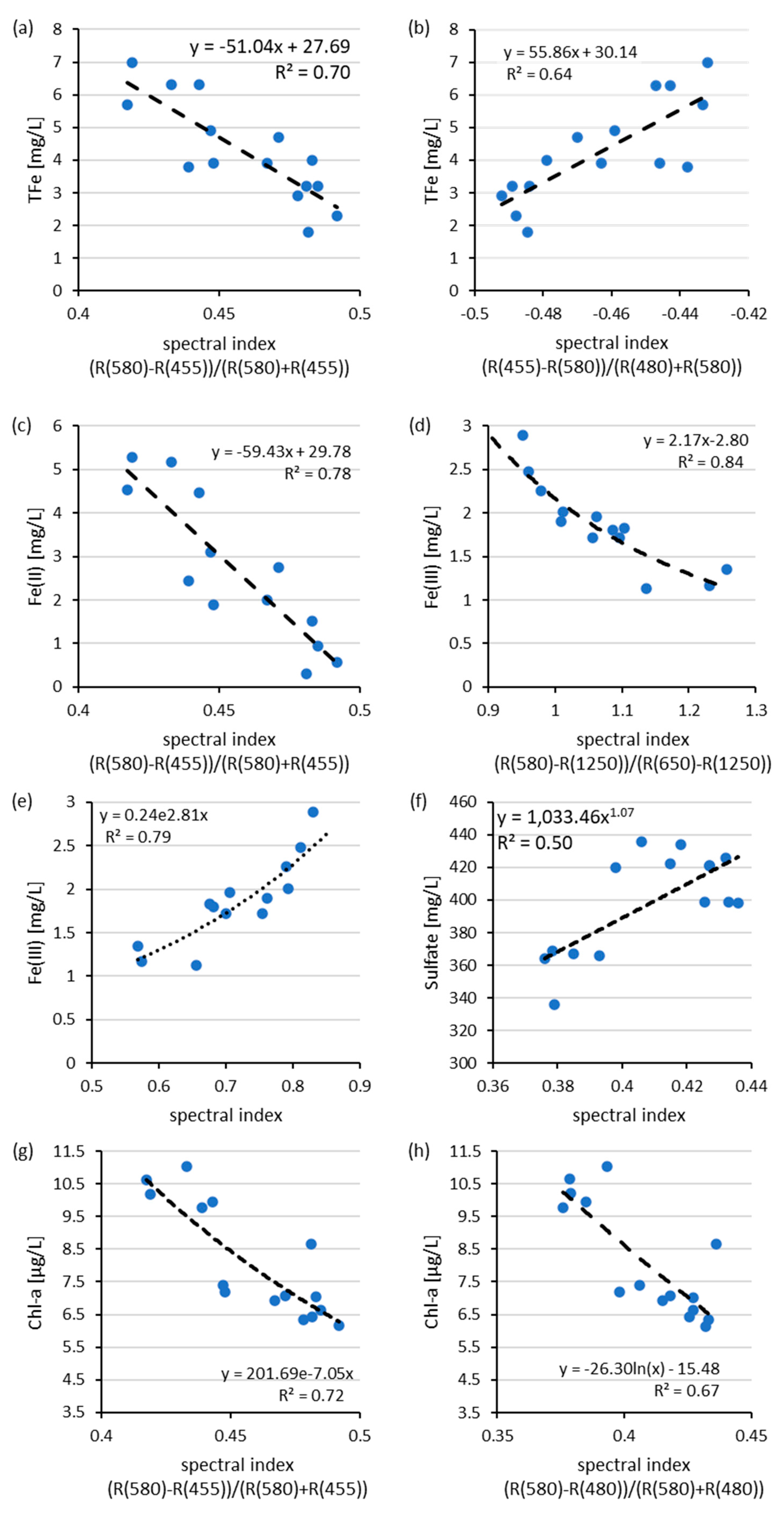
3.2. Airborne Hyperspectral RS and Modelling

Thanks to the institute’s own gyrocopter with the hyperspectral sensor technology HySpex, it was possible to record airborne hyperspectral images in the wavelength range from 420 to 1500 nm at the same time as the in situ measurements. Figure 6 shows the results of the refluxes in the wavelength range from 440 to 1400 nm at five in situ measuring points for which airborne hyperspectral RS was conducted.

Figure 6 clearly shows that the reflectance in the wavelength range from 560 to 700 nm increased with increasing iron(III) concentration. This can also be seen from the correlation of R² = 0.78 with the wavelength at 675 nm (see

Table 3. List of the area coverage derivation results showing the number of samples used (N), the ID to link to the regression models in Figure 1, the spectral index, the regression equation, the coefficient of determination (R²), the RMSE and the rRMSE. The models displayed in bold font were used in Figure 6 for the specific concentration derivation.

Parameter	N	ID	Spectral Index	Equation	R2	RMSE	rRMSE
TFe [mg/L]	15	(a)	(RRS(580)-RRS(455))/(RRS(580)+RRS(455))	$\widehat{p}=51.04\times \left(\frac{R_1}{R_2}\right)+27.69$	0.70	0.95	22.19%
		(b)	(RRS(455)-RRS(580))/(RRS(480)+RRS(580))	$\widehat{\mathit{p}}=\mathbf{55.86}\times \left(\frac{{\mathit{R}}_{\mathbf{1}}}{{\mathit{R}}_{\mathbf{2}}}\right)+\mathbf{30.14}$	0.64	0.93	21.91%
Fe(II) [mg/L]	13	(c)	(RRS(580)-RRS(455))/(RRS(580)+RRS(455))	$\widehat{\mathit{p}}=\mathbf{59.43}\times \left(\frac{{\mathit{R}}_{\mathbf{1}}}{{\mathit{R}}_{\mathbf{2}}}\right)+\mathbf{29.78}$	0.78	0.95	35.33%
Fe(III) [mg/L]	13	(d)	(RRS(580)-RRS(1250))/(RRS(650)-RRS(1250))	$\widehat{p}=2.17\times {\left(SI\right)}^{-2.8}$	0.84	0.27	14.53%
		(e)	RRS(701)/RRS(563)	$\widehat{\mathit{p}}=\mathbf{0.24} {\mathit{e}}^{\mathbf{2.81}\left(\mathit{S}\mathit{I}\right)}$	0.79	0.22	11.86%
Sulphate [mg/L]	15	(f)	(RRS(580)-RRS(480))/(RRS(580)+RRS(480))	$\widehat{\mathit{p}}=\mathbf{1.03}\times {\left(\mathit{S}\mathit{I}\right)}^{\mathbf{1.07}}$	0.53	21	5.31%
Chl-a [µg/L]	15	(g)	(RRS(580)-RRS(455))/(RRS(580)+RRS(455))	$\widehat{p}=201.69 e^{-7.05\left(SI\right)}$	0.72	1.09	13.48%
		(h)	(RRS(580)-RRS(480))/(RRS(580)+RRS(480))	$\widehat{\mathit{p}}=\mathbf{26.3}\times \mathit{l}\mathit{n}\left(\mathit{S}\mathit{I}\right)-\mathbf{15.48}$	0.67	0.98	12.09%

). Within the wavelength range of 400–560 nm, the aRRS was low owing to absorption by CDOM and Chl-a [32]. In addition, Weyhenmeyer et al. [70] observed that Fe(II), like DOC, correlates with absorption at 420 nm. Moreover, according to Asmala et al. [31], the influence of Fe(II) on the absorption behaviour of the water body is visible beyond 520 nm. However, based on the acquired data, the spectral influence of Fe(II) and sulphate was not visible within this wavelength range. This was particularly due to the rapid oxidation of Fe(II) to Fe(III). In addition, in the spectral range of 560–700 nm, most maxima exceeding 6% could be determined at the measuring points with a TFe concentration exceeding 3 mg/L. The highest maximum at 580 nm shows the spectrum of SP 16 with the highest Fe(III) concentration of 2.89 mg/L (see Figure 6a). Owing to the high concentration of Fe(III) and the resulting flocculation, the water became very turbid, which, according to Frauendorf [30], makes Fe(III) classifiable as TSM.

By means of the multi-spectrometer Ocean and Land Colour Instrument (OLCI) on board the Sentinel 3, Knaeps et al. [71] established that with increasing TSM concentration up to 402 mg/L, additional information on the short-wave infrared (SWIR) range contributes to more accurate modelling. Furthermore, iron compounds in the soil show specific spectral characteristics, especially in the SWIR range [72]. The spectra with a TFe concentration under 3 mg/L are similar to the aRRS of natural rivers (SP 19 in Figure 6). Absorption by water is clearly visible between 700–1000 nm. The aRRS between 1000–1615 nm do not show additional information.

The most suitable regression models to link particular spectral indices to water constituents are shown in Figure 7. They are also displayed in Table 3, which additionally shows the number of samples used, the spectral index, the ID to link to the regression models, the regression equation, R², the RMSE and the rRMSE. The number of samples for modelling was lower than indicated because not every sampling location was within the coverage area of the RS data. The empirical models achieved a derivation accuracy of 0.93 mg/L for the total iron concentration, 0.95 mg/L for ferrous iron, 0.22 mg/L for ferric iron and 21 mg/L for sulphate.

Both indices for the derivation of TFe were based on the wavelengths of 455 and 580 nm and can be explained based on spectral analysis. The wavelength range between 450–500 nm was characterized by a broad absorption band of iron oxides. This was also confirmed by Rowan and Goetz [72]. As shown in Figure 7, there was a maximum in the reflectance at 580 nm, which was caused by an increased scattering by TSM and a low absorption by Chl-a [32,73]. Since TFe and Chl-a are correlated, it is difficult to distinguish between these constituents based on regression models. A linear regression of the single wavelength at 580 nm and TFe and Chl-a (Equations (1) and (6)) shows that the reflection decreased with increasing TFe (r² = 0.5) and Chl-a (r² = 0.3) concentrations, indicating that iron was mainly responsible for the optical properties within this wavelength range.

As a result, there was a steep slope from 450–580 nm in the spectral curve. The most suitable model for deriving the TFe content obtained an rRMSE of 21.91% and an R² of 0.64. The regression model for determining the Fe(II) concentration with the highest correlation of 0.78 was based on the same spectral analysis as TFe but the validation showed a higher rRMSE of 35.33%. The use of the same spectral index as the basis for the derivation model can be explained by the high correlation r = 0.97 between TFe and Fe(II). The first model for the derivation of Fe(III) was based on the study conducted by Knaeps et al. [46] and is suitable for inland waters with a TSM concentration of 30 to 1400 mg/L. The index showed an R² of 0.80 and an rRMSE of 14.53%. The second model used to derive Fe(III) was based on the spectral index RRS(701)/RRS(563) and yielded an accuracy of 11.86% and an R² of 0.76. According to Gitelson [32], this index is suitable for deriving Chl-a. However, spectral analyses with the software package WASI [74] showed that the reflectance increases around 580 nm with increasing TSM concentration. Furthermore, the absorption by water increased steadily from 700 nm, resulting in a strong reduction in reflectance. As a result, there was a strong gradient between 580 and 700 nm.

The model used to derive sulphate yielded an R² = 0.53 and an rRMSE of 5.31%. The derivation algorithm used a potential regression model based on the spectral index (RRS(580)-RRS(480))/(RRS(580)+RRS(480)). This spectral index was based on the analyses carried out. As described, there was an increased scattering at 580 nm owing to the TSM concentration [32]. Furthermore, the aforementioned absorption of iron oxides at the 480 nm range contributed to a strong gradient in the 480–580 nm range.

The spectral indices obtained for the derivation of Chl-a were similar to those of the derivation of TFe. This was probably related to the high correlation of r = 0.79 between Chl-a and TFe, as well as Fe(II). Nevertheless, the best fitting regression model was (RRS(580) − RRS(480))/(RRS(580) + RRS(480)) based on a logarithmic approach and a derivative accuracy of RMSE = 0.98 µg/L.

To summarize, it was concluded that the derivative models, with the exception of Fe(III), mainly referred to the spectral range from 450 to 580 nm. Based on the day of the investigation, this spectral range had the highest derivation accuracy. Wavelengths beyond 560 nm were only considered for the derivation of Fe(III).

Figure 8 shows the derivation results of TFe, Fe(II), Fe(III), sulphate and Chl-a using three different locations as examples (see Figure 1). The background of the derivation results consisted of channels 580, 680 and 780 nm of the hyperspectral image. Therefore, the River Spree and the Spremberg Dam appeared blue. Masked areas are shown in black. Areas outside of the water body are displayed in grey. Data-free areas are presented in white. For the derivation of the water constituents TFe, Fe(II), Fe(III), sulphate and Chl-a, the models displayed in bold in Table 3 were used.

Figure 8 shows the mouth of the Kleine Spree into the River Spree. Based on the derivation results of TFe (see Figure 8(a-II)), a difference was observed between the concentration in the Kleine Spree and that in the River Spree. In the case of Fe(II) derivation (see Figure 8(a-III)), the influence of the Kleine Spree was comparatively low. The influence of the Kleine Spree River can only be observed directly at the river mouth based on Chl-a derivatives (see Figure 8(a-VI)). The derived Fe(III) (see Figure 8(a-IV)) and sulphate (see Figure 8(a-V)) concentrations showed no visible change. In the case of Fe(III), this could be attributed to the low oxygen saturation in the Kleine Spree River, as observed by Uhlmann et al. [52], whereby only a small amount of Fe(II) was oxidised.

Figure 8 column b shows the mouth area of the industrial canal from the Schwarze Pumpe industrial park. A clear increase in the sulphate concentration can be seen there (see Figure 8(b-V)). Based on the derived TFe (see Figure 8(b-II)), Fe(II) (see Figure 8(b-III)) and Chl-a (see Figure 8(b-VI)) concentrations, a decrease in the mouth area of the industrial canal was first identified. After that, the concentration rose. From the Fe(III) concentration shown (see Figure 8(b-IV)), no change was detected.

Figure 8 column c displays the mouth of the Spree into the Spremberg reservoir. Owing to chemical and spectral differences between the River Spree and the southern part of the Spremberg reservoir, no suitable concentrations could be derived. Nevertheless, clear differences between the River Spree and the Spremberg reservoir were observed, except for the derivation result of Fe(III) (see Figure 8(c-IV)). Thus, the derived TFe concentration clearly showed that the River Spree only had a low TFe concentration after the upstream pre-dam Bühlow (see Figure 8(c-II)). This concentration increased in the Spremberg reservoir. Similar observations were made with respect to the Fe(II) (see Figure 8(c-III)) and Chl-a (see Figure 8(c-IV)) concentrations. However, the derived sulphate concentration was different (see Figure 8(c-V)). In the resulting image, the River Spree shows a very high concentration and the reservoir initially exhibited a low concentration. This raises the possibility that another source of iron input was located south of the Spremberg reservoir, such as swamps that were drained during open-cast mining activities.

4. Conclusions and Outlook

In this study, a combination of airborne imaging hyperspectral/RGB-RS was used to monitor water quality parameters of smaller rivers that were altered by open-cast mining processes with subsequent renaturation and groundwater recharge. The focus of monitoring, modelling and prediction was on the water quality variables TFe, Fe(II), Fe(III), sulphate and Chl-a. Due to the availability of a university-owned gyrocopter with corresponding RS sensors (HySpex, RGB, TIR), simultaneous imaging airborne RS data and in situ measurement data could be collected on site in the Spree.

The acquisition of simultaneous RGB data guaranteed the creation of a highly accurate terrain model, which was urgently needed for processing (geometric correction of) airborne hyperspectral data. With this approach, airborne hyperspectral RS and in situ data could be used for the first time to separately derive the water quality indicators Fe(II) and Fe(III) for smaller streams with neutral pH by means of regression. They were then modelled and the point measurements were transferred into space. The determination of the total iron concentration in open-cast mining lakes was already carried out by numerous studies, but the differentiation between the types Fe(II) and Fe(III) had not yet been made in any study available so far. This was partly due to the very low concentration of Fe(III) in the open-cast mining lakes. In addition, the examples on AMDs showed that iron could be identified, but no concentrations have been derived directly; therefore, the results should only be understood as an index. Furthermore, the advantage of our study was that in situ measurements could be conducted at the same time as hyperspectral measurements (400–2500 nm). Especially in rapidly changing aquatic systems, this method was found to be useful. The empirical models achieved a derivation accuracy of 0.93 mg/L for the total iron concentration, 0.95 mg/L (R² = 64%) for iron, 0.22 mg/L (R² = 79%) for ferric iron and 21 mg/L (R² = 64%) for sulphate (R² = 53%). An empirical approach was chosen for the study because it was robust; could be implemented quickly; and, with the focus on sulphate, was particularly target-oriented.

The obvious disadvantages, such as its low transferability and high statistical dependence, were taken into account by investigating a large number of spectral indices and using a valid statistical evaluation from the coefficient of determination and RMSE value. This also avoided an overspecialisation of the algorithm. The derivation results shown in Figure 8 demonstrate how inflowing river water could be clearly distinguished from reservoir water and how local phenomena, such as inflowing channels or rivers, could be reliably detected. This underlines the applicability of airborne RS for smaller flowing waters for continuous water quality monitoring.

The general conditions and requirements were as follows:

• The present results were only achieved by combining airborne hyperspectral RS data with simultaneous in situ measurements.
• Airborne hyperspectral sensors acquire very high-resolution and continuous spectra that allow detailed analyses to be carried out. The high spatial resolution offers significant advantages over satellite data (multispectral and hyperspectral) with a low spatial resolution for the derivation of water constituents from inland waters.
• Machine learning methods must be applied rather than simple regression models for modelling and prediction to achieve a better generalisation and transferability of the results.
• Spectral databases need to be in place for the quantification of water quality indicators.
• Scale dependencies have to be undertaken to transfer from high-resolution airborne hyperspectral RS data to the now freely available spaceborne hyperspectral data (EnMAP, DESIS, Prisma).

The method has tremendous potential to be practically established and transferred into official monitoring procedures in order to combine official in situ measurements with airborne and spaceborne RS information and to achieve added value for the monitoring of water quality indicators.

References

1. Van Dijk, A.I.J.M.; Beck, H.E.; de Jeu, R.A.M.; Dorigo, W.A.; Hou, J.; Preimesberger, W.; Rahman, J.; Rozas Larraondo, P.R.; Van Der, R.S. Global Water Monitor 2022, Summary Report. Global Water Monitor. Available online: www.globalwater.online (accessed on 3 March 2023).
2. Tiwary, R.K. Environmental Impact of Coal Mining Onwater Regime and Its Management. Water. Air. Soil Pollut. 2001, 132, 185–199. [Google Scholar] [CrossRef]
3. Margareta, M.; Kaartinen, T.; Mäkinen, J.; Punkkinen, H.; Häkkinen, A.; Mamelkina, M.; Tuunila, R.; Lamberg, P.; Gonzales, M.S.; Sandru, M.; et al. Water Conscious Mining (WASCIOUS); TemaNord; Nordic Council of Ministers: Copenhagen, Denmark, 2017; ISBN 9789289349628. [Google Scholar]
4. España, J.S. Acid Mine Drainage in the Iberian Pyrite Belt: An Overview with Special Emphasis on Generation Mechanisms, Aqueous Composition and Associated Mineral Phases. In Proceedings of the Conferencia Invitada: Sánchez España, Macla, Spain, Madrid; 2008; Volume 10, pp. 34–43. Available online: https://www.researchgate.net/publication/235355094_Acid_Mine_Drainage_in_the_Iberian_Pyrite_Belt_an_Overviewwith_Special_Emphasis_on_Generation_MechanismsAqueous_Composition_and_Associated_Mineral_Phases (accessed on 1 February 2023).
5. Schultze, M.; Pokrandt, K.-H.; Hille, W. Pit lakes of the Central German lignite mining district: Creation, morphometry and water quality aspects. Limnologica 2010, 40, 148–155. [Google Scholar] [CrossRef]
6. Bilek, F.; Koch, C. Eisenretention in der Talsperre Spremberg, 2012. Available online: https://lfu.brandenburg.de/lfu/de/ueber-uns/veroeffentlichungen/detail/~31-10-2012-eisenretention-in-der-talsperre-spremberg (accessed on 1 February 2023).
7. Giam, X.; Olden, J.D.; Simberloff, D. Impact of coal mining on stream biodiversity in the US and its regulatory implications. Nat. Sustain. 2018, 1, 176–183. [Google Scholar] [CrossRef]
8. Hüttl, R.F. Ecology of post strip-mining landscapes in Lusatia, Germany. Environ. Sci. Policy 1998, 1, 129–135. [Google Scholar] [CrossRef]
9. Zerbe, S.; Wiegleb, G. Renaturierung von Ökosystemen in Mitteleuropa; Zerbe, S., Wiegleb, G., Eds.; Spektrum Akademischer Verlag: Heidelberg, Germany, 2009; ISBN 978-3-8274-1901-9. [Google Scholar]
10. Lunt, J.; Smee, D.L. Turbidity alters estuarine biodiversity and species composition. ICES J. Mar. Sci. 2020, 77, 379–387. [Google Scholar] [CrossRef]
11. Ramadas, M.; Samantaray, A.K. Applications of Remote Sensing and GIS in Water Quality Monitoring and Remediation: A State-of-the-Art Review. In Water Remediation; Springer Nature: Singapore, 2018; pp. 225–246. [Google Scholar]
12. Sagan, V.; Peterson, K.T.; Maimaitijiang, M.; Sidike, P.; Sloan, J.; Greeling, B.A.; Maalouf, S.; Adams, C. Monitoring inland water quality using remote sensing: Potential and limitations of spectral indices, bio-optical simulations, machine learning, and cloud computing. Earth-Sci. Rev. 2020, 205, 103187. [Google Scholar] [CrossRef]
13. Olmanson, L.G.; Brezonik, P.L.; Bauer, M.E. Airborne hyperspectral remote sensing to assess spatial distribution of water quality characteristics in large rivers: The Mississippi River and its tributaries in Minnesota. Remote Sens. Environ. 2013, 130, 254–265. [Google Scholar] [CrossRef]
14. Chawla, I.; Karthikeyan, L.; Mishra, A.K. A review of remote sensing applications for water security: Quantity, quality, and extremes. J. Hydrol. 2020, 585, 124826. [Google Scholar] [CrossRef]
15. Gholizadeh, M.; Melesse, A.; Reddi, L. A Comprehensive Review on Water Quality Parameters Estimation Using Remote Sensing Techniques. Sensors 2016, 16, 1298. [Google Scholar] [CrossRef]
16. Ritchie, J.C.; Zimba, P.V.; Everitt, J.H. Remote Sensing Techniques to Assess Water Quality. Photogramm. Eng. Remote Sens. 2003, 69, 695–704. [Google Scholar] [CrossRef]
17. Göritz, A.; Berger, S.; Gege, P.; Grossart, H.-P.; Nejstgaard, J.; Riedel, S.; Röttgers, R.; Utschig, C. Retrieval of Water Constituents from Hyperspectral In-Situ Measurements under Variable Cloud Cover—A Case Study at Lake Stechlin (Germany). Remote Sens. 2018, 10, 181. [Google Scholar] [CrossRef]
18. Pan, X.; Wang, Z.; Ullah, H.; Chen, C.; Wang, X.; Li, X.; Li, H.; Zhuang, Q.; Xue, B.; Yu, Y. Evaluation of Eutrophication in Jiaozhou Bay via Water Color Parameters Determination with UAV-Borne Hyperspectral Imagery. Atmosphere 2023, 14, 387. [Google Scholar] [CrossRef]
19. Kakuta, S.; Ariyasu, E.; Takeda, T. Shallow Water Bathymetry Mapping Using Hyperspectral Data. In Proceedings of the IGARSS 2018—2018 IEEE International Geoscience and Remote Sensing Symposium, Valencia, Spain, 22–27 July 2018; pp. 1539–1542. [Google Scholar]
20. Alonso, K.; Bachmann, M.; Burch, K.; Carmona, E.; Cerra, D.; de los Reyes, R.; Dietrich, D.; Heiden, U.; Hölderlin, A.; Ickes, J.; et al. Data Products, Quality and Validation of the DLR Earth Sensing Imaging Spectrometer (DESIS). Sensors 2019, 19, 4471. [Google Scholar] [CrossRef] [PubMed]
21. Guanter, L.; Kaufmann, H.; Segl, K.; Foerster, S.; Rogass, C.; Chabrillat, S.; Kuester, T.; Hollstein, A.; Rossner, G.; Chlebek, C.; et al. The EnMAP Spaceborne Imaging Spectroscopy Mission for Earth Observation. Remote Sens. 2015, 7, 8830–8857. [Google Scholar] [CrossRef]
22. Lopinto, E.; Fasano, L.; Longo, F.; Varacalli, G.; Sacco, P.; Chiarantini, L.; Sarti, F.; Agrimano, L.; Santoro, F.; Cogliati, S.; et al. Current Status and Future Perspectives of the PRISMA Mission at the Turn of One Year in Operational Usage. In Proceedings of the 2021 IEEE International Geoscience and Remote Sensing Symposium IGARSS, Brussels, Belgium, 11–16 July 2021; pp. 1380–1383. [Google Scholar]
23. Imatani, R.; Ito, Y.; Ikehara, K.; Iwasaki, A.; Inada, H.; Tanii, J.; Kashimura, O. The flight model performances of Hyperspectral Imager Suite (HISUI). In Proceedings of the Sensors, Systems, and Next-Generation Satellites XXV, Online Conference, Spain; 2021; p. 3. Available online: https://ui.adsabs.harvard.edu/abs/2021SPIE11858E..08I/abstract (accessed on 1 February 2023).
24. Gege, P. Radiative Transfer Theory for Inland Waters. In Bio-Optical Modeling and Remote Sensing of Inland Waters; Elsevier: Amsterdam, The Netherlands, 2017; pp. 25–67. ISBN 978-0-12-804644-9. [Google Scholar]
25. Ogashawara, I.; Mishra, D.R.; Gitelson, A.A. Remote Sensing of Inland Waters. In Bio-Optical Modeling and Remote Sensing of Inland Waters; Elsevier: Amsterdam, The Netherlands, 2017; pp. 1–24. ISBN 978-0-12-804644-9. [Google Scholar]
26. Dörnhöfer, K.; Oppelt, N. Remote sensing for lake research and monitoring—Recent advances. Ecol. Indic. 2016, 64, 105–122. [Google Scholar] [CrossRef]
27. Dekker, A.G. Detection of Optical Water Quality Parameters for Eutrophic Waters by High Resolution Remote Sensing. Ph.D. Thesis, Free University, Berlin, Germany, 1993. [Google Scholar]
28. Matthews, M.W. A current review of empirical procedures of remote sensing in inland and near-coastal transitional waters. Int. J. Remote Sens. 2011, 32, 6855–6899. [Google Scholar] [CrossRef]
29. Kirk, J.T.O. Light and Photosynthesis in Aquatic Ecosystems; 3. Auflage.; Cambridge University Press: Canberra, Australia, 2010; ISBN 978-0-521-15175-7. [Google Scholar]
30. Frauendorf, J. Entwicklung und Anwendung von Fernerkundungsmethoden zur Ableitung von Wasserqualitätsparametern verschiedener Restseen des Braunkohlentagebaus in Mitteldeutschland; Martin-Luther-Universität Halle-Wittenberg: Halle, Germany, 2002. [Google Scholar] [CrossRef]
31. Asmala, E.; Stedmon, C.A.; Thomas, D.N. Linking CDOM spectral absorption to dissolved organic carbon concentrations and loadings in boreal estuaries. Estuar. Coast. Shelf Sci. 2012, 111, 107–117. [Google Scholar] [CrossRef]
32. Gitelson, A.A. The peak near 700 nm on radiance spectra of algae and water: Relationships of its magnitude and position with chlorophyll concentration. Int. J. Remote Sens. 1992, 13, 3367–3373. [Google Scholar] [CrossRef]
33. Kopačková, V.; Hladíková, L. Applying Spectral Unmixing to Determine Surface Water Parameters in a Mining Environment. Remote Sens. 2014, 6, 11204–11224. [Google Scholar] [CrossRef]
34. Repic, R.L.; Lee, J.K.; Mausel, P.W. An Analysis of Selected Water Parameters in Surface Coal Mines Using Multispectral Videography. Photogramm. Eng. 1991, 4, 1589–1596. [Google Scholar]
35. Anderson, J.E.; Robbins, E. Spectral Reflectance and Detection of Iron-Oxide Precipitates Associated with Acidic Mine Drainage. Photogramm. Eng. Remote Sens. 1998, 64, 1201–1208. [Google Scholar]
36. Williams, D.J.; Bigham, J.M.; Cravotta III, C.A.; Trainaa, S.J.; Anderson, J.E.; Lyon, J.G. Assessing mine drainage pH from the color and spectral reflectance of chemical precipitates. Appl. Geochem. 2002, 17, 1273–1286. [Google Scholar] [CrossRef]
37. Gläßer, C.; Groth, D.; Frauendorf, J. Monitoring of hydrochemical parameters of lignite mining lakes in Central Germany using airborne hyperspectral casi-scanner data. Int. J. Coal Geol. 2011, 86, 40–53. [Google Scholar] [CrossRef]
38. Schroeter, L.; Gläβer, C. Analyses and monitoring of lignite mining lakes in Eastern Germany with spectral signatures of Landsat TM satellite data. Int. J. Coal Geol. 2011, 86, 27–39. [Google Scholar] [CrossRef]
39. Brando, V.E.; Dekker, A.G. Satellite hyperspectral remote sensing for estimating estuarine and coastal water quality. IEEE Trans. Geosci. Remote Sens. 2003, 41, 1378–1387. [Google Scholar] [CrossRef]
40. Bukata, R.P.; Jerome, J.H.; Kondratyev, K.Y.; Pozdnyakov, D.V. Optical Properties and Remote Sensing of Inland and Coastal Waters; CRC Press: Boca Raton, FL, USA, 2018; ISBN 9780203744956. [Google Scholar]
41. Kutser, T.; Hedley, J.; Giardino, C.; Roelfsema, C.; Brando, V.E. Remote sensing of shallow waters—A 50 year retrospective and future directions. Remote Sens. Environ. 2020, 240, 111619. [Google Scholar] [CrossRef]
42. Kuhn, C.; de Matos Valerio, A.; Ward, N.; Loken, L.; Sawakuchi, H.O.; Kampel, M.; Richey, J.; Stadler, P.; Crawford, J.; Striegl, R.; et al. Performance of Landsat-8 and Sentinel-2 surface reflectance products for river remote sensing retrievals of chlorophyll-a and turbidity. Remote Sens. Environ. 2019, 224, 104–118. [Google Scholar] [CrossRef]
43. Balasubramanian, S.V.; Pahlevan, N.; Smith, B.; Binding, C.; Schalles, J.; Loisel, H.; Gurlin, D.; Greb, S.; Alikas, K.; Randla, M.; et al. Robust algorithm for estimating total suspended solids (TSS) in inland and nearshore coastal waters. Remote Sens. Environ. 2020, 246, 111768. [Google Scholar] [CrossRef]
44. Baschek, B.; Fricke, K.; Dörnhöfer, K.; Oppelt, N. Grundlagen und Möglichkeiten der passiven Fernerkundung von Binnengewässern. In Handbuch Angewandte Limnologie: Grundlagen—Gewässerbelastung—Restaurierung—Aquatische Ökotoxikologie—Bewertung—Gewässerschutz; Wiley: Hoboken, NJ, USA, 2018; pp. 1–28. ISBN 978-3-527-67848-8. [Google Scholar]
45. Doxaran, D.; Froidefond, J.-M.; Castaing, P. Remote-sensing reflectance of turbid sediment-dominated waters Reduction of sediment type variations and changing illumination conditions effects by use of reflectance ratios. Appl. Opt. 2003, 42, 2623. [Google Scholar] [CrossRef]
46. Knaeps, E.; Ruddick, K.G.; Doxaran, D.; Dogliotti, A.I.; Nechad, B.; Raymaekers, D.; Sterckx, S. A SWIR based algorithm to retrieve total suspended matter in extremely turbid waters. Remote Sens. Environ. 2015, 168, 66–79. [Google Scholar] [CrossRef]
47. Friedland, G.; Grüneberg, B.; Hupfer, M. Geochemical signatures of lignite mining products in sediments downstream a fluvial-lacustrine system. Sci. Total Environ. 2021, 760, 143942. [Google Scholar] [CrossRef]
48. Bilek, F.; Moritz, F.; Albinus, S. Iron-Hydroxide-Removal from Mining Affected Rivers. In Proceedings of the Mining Meets Water—Conflicts and Solutions; International Mine Water Association (IMWA): Freiberg, Germany, 2016; pp. 151–158. [Google Scholar]
49. Gleisner, M.; Herbert, R.B. Sulfide mineral oxidation in freshly processed tailings: Batch experiments. J. Geochem. Explor. 2002, 76, 139–153. [Google Scholar] [CrossRef]
50. Uhlig, U.; Radigk, S.; Uhlmann, W.; Preuß, V.; Koch, T. Iron removal from the Spree River in the Bühlow pre-impoundment basin of the Spremberg reservoir IMWA 2016. Available online: https://www.imwa.info/docs/imwa_2016/IMWA2016_Uhlig_75.pdf (accessed on 1 February 2023).
51. Uhlmann, W.; Theiss, S.; Nestler, W.; Claus, T. Fortführung der Studie zur Talsperre Spremberg—Abschlussbericht (Dezember 2013). Available online: https://docplayer.org/83470767-Fortfuehrung-der-studie-zur-talsperre-spremberg-abschlussbericht-dezember-2013.html (accessed on 1 February 2023).
52. Uhlmann, W.; Theiss, S.; Nestler, W.; Zimmermann, K.; Claus, T. Weiterführende Untersuchungen zu den Hydrochemischen und Ökologischen Auswirkungen der Exfiltration von Eisenhaltigem, Saurem Grundwasser in die Kleine Spree und in Die Spree Projektphase 2: Präzisierung der Ursachen und Quellstärken für die Hohe Eisenbel; IWB: Dresden, Germany, 2012. [Google Scholar]
53. LMBV LMBV: Spree bei Wilhelmsthal bekommt wieder Kalk—Übergang in Spätsommer-Fahrweise. Available online: https://www.lmbv.de/index.php/pressemitteilung/lmbv-spree-bei-wilhelmsthal-bekommt-wieder-kalk-uebergang-in-spaetsommer-fahrweise-4576.html (accessed on 1 February 2023).
54. Mehnert, G.; Rücker, J.; Nicklisch, A.; Leunert, F.; Wiedner, C. Effects of thermal acclimation and photoacclimation on lipophilic pigments in an invasive and a native cyanobacterium of temperate regions. Eur. J. Phycol. 2012, 47, 182–192. [Google Scholar] [CrossRef]
55. Schonberger, J.L.; Frahm, J.-M. Structure-from-Motion Revisited. In Proceedings of the 2016 IEEE Conference on Computer Vision and Pattern Recognition (CVPR), Las Vegas, NV, USA, 27–30 June 2016; pp. 4104–4113. [Google Scholar]
56. Schläpfer, D. PARGE Airborne Image Rectification PARGE® Image Rectification. 2022. Available online: https://www.rese-apps.com/software/parge/index.html (accessed on 1 February 2023).
57. Schläpfer, D. ATCOR for Airborne Remote Sensing. ATCOR 4—For Airborne Remote Sensing Systems. 2022. Available online: https://www.rese-apps.com/software/atcor-4-airborne/index.html (accessed on 1 February 2023).
58. Hovis, W.A.; Leung, K.C. Remote Sensing of Ocean Color. Opt. Eng. 1977, 16, 439–472. [Google Scholar] [CrossRef]
59. Ray, T.W. A FAQ on Vegetation in Remote Sensing, 1994, IEEE/ACM Third International Conference on Cyber-Physical Systems. Pasadena. 1994. Available online: http://www.remote-sensing.info/wp-content/uploads/2012/07/A_FAQ_on_Vegetation_in_Remote_Sensing.pdf (accessed on 1 February 2023).
60. Moses, W.J.; Sterckx, S.; Montes, M.J.; De Keukelaere, L.; Knaeps, E. Atmospheric Correction for Inland Waters. In Bio-Optical Modeling and Remote Sensing of Inland Waters; Elsevier: Amsterdam, The Netherlands, 2017; pp. 69–100. ISBN 978-0-12-804644-9. [Google Scholar]
61. Håkanson, L.; Bryhn, A.C.; Blenckner, T. Operational Effect Variables and Functional Ecosystem Classifications—A Review on Empirical Models for Aquatic Systems along a Salinity Gradient. Int. Rev. Hydrobiol. 2007, 92, 326–357. [Google Scholar] [CrossRef]
62. Ulrich, C.; Bannehr, L.; Lausch, A. Ableitung von Eisen(II, III)oxid in Fließgewässern mittels Multispektraldaten. In Proceedings of the Gesellschaft für Photogrammetrie, Fernerkundung und Geoinformation, Bern, Switzerland; 2016; Volume 25, pp. 34–43. Available online: https://www.google.com.hk/search?q=Ableitung+von+Eisen%28II%2C+III%29oxid+in+Flie%C3%9Fgew%C3%A4ssern+mittels+Multispektraldaten&ei=JL83ZOaWDb-m2roP7qah8Ao&ved=0ahUKEwjmuNmCuqb-AhU_k1YBHW5TCK4Q4dUDCA4&uact=5&oq=Ableitung+von+Eisen%28II%2C+III%29oxid+in+Flie%C3%9Fgew%C3%A4ssern+mittels+Multispektraldaten&gs_lcp=Cgxnd3Mtd2l6LXNlcnAQA0oECEEYAFAAWABgiQNoAHABeACAAXmIAXmSAQMwLjGYAQCgAQKgAQHAAQE&sclient=gws-wiz-serp (accessed on 1 February 2023).
63. Durning, W.P.; Polis, S.R.; Frost, E.G.; Kaiser, J.V. Integrated Use of Remote Sensing and GIS for Mineral Exploration-Final Report. Affiliated Research Center, San Diego State University: San Diego, CA, USA, 1998. [Google Scholar]
64. Eloheimo, K.; Hannonen, T.; Härmä, P.; Pyhälahti, T.; Koponen, S.; Pulliainen, J.; Servomaa, H.; Kutser, T. Coastal monitoring using satellite, airborne and in situ data in the archipelago of Baltic Sea. In Proceedings of the 5th International Conference on Remote Sensing for Marine and Coastal Environments, San Diego, CA, USA, 5–7 October 1998; pp. 306–331. [Google Scholar]
65. Robinson, M.-C.; Morris, K.P.; Dyer, K.R. Deriving Fluxes of Suspended Particulate Matter in the Humber Estuary, UK, Using Airborne Remote Sensing. Mar. Pollut. Bull. 1999, 37, 155–163. [Google Scholar] [CrossRef]
66. van der Meer, F.D.; van der Werff, H.M.A.; van Ruitenbeek, F.J.A. Potential of ESA’s Sentinel-2 for geological applications. Remote Sens. Environ. 2014, 148, 124–133. [Google Scholar] [CrossRef]
67. IOCCG. Remote Sensing of Ocean Colour in Coastal, and Other Optically-Complex, Waters, Reports of the International Ocean-Colour Coordinating Group. Reports of the International Ocean-Colour Coordinating Group, Dartmouth, Kanada. 2020. Available online: http://ioccg.org/wp-content/uploads/2015/10/ioccg-report-03.pdf (accessed on 1 February 2023).
68. Gao, H.; Birkett, C.; Lettenmaier, D.P. Global monitoring of large reservoir storage from satellite remote sensing. Water Resour. Res. 2012, 48, 2012WR012063. [Google Scholar] [CrossRef]
69. Wang, J.-J.; Lu, X.X. Estimation of suspended sediment concentrations using Terra MODIS: An example from the Lower Yangtze River, China. Sci. Total Environ. 2010, 408, 1131–1138. [Google Scholar] [CrossRef]
70. Weyhenmeyer, G.A.; Prairie, Y.T.; Tranvik, L.J. Browning of Boreal Freshwaters Coupled to Carbon-Iron Interactions along the Aquatic Continuum. PLoS ONE 2014, 9, e88104. [Google Scholar] [CrossRef]
71. Knaeps, E.; Dogliotti, A.I.; Raymaekers, D.; Ruddick, K.; Sterckx, S. In situ evidence of non-zero reflectance in the OLCI 1020 nm band for a turbid estuary. Remote Sens. Environ. 2012, 120, 133–144. [Google Scholar] [CrossRef]
72. Rowan, L.C.; Goetz, A.F.H.; Ashley, R.P. Discrimination of hydrothermallyy altered and unaltered rocks in visible and near infrared multispectral images. Geophysics 1977, 42, 522–535. [Google Scholar] [CrossRef]
73. Haardt, H.; Maske, H. Specific in vivo absorption coefficient of chlorophyll a at 675 nm1. Limnol. Oceanogr. 1987, 32, 608–619. [Google Scholar] [CrossRef]
74. Gege, P. The water colour simulator WASI: A software tool for forward and inverse modeling of optical in-situ spectra. In Proceedings of the IGARSS 2001. Scanning the Present and Resolving the Future. Proceedings. IEEE 2001 International Geoscience and Remote Sensing Symposium (Cat. No.01CH37217), Sydney, Australia, 9–13 July 2001; Volume 6, pp. 2743–2745. [Google Scholar]
Figure 1. Study site in the south-east of Berlin in Lusatia along the Spree River from the Ruhlmühle village to the Spremberg reservoir. The flow direction of the Spree from south to north. (a–c) shows the sites for more in-depth studies.
Water 15 01532 g001
Figure 2. Schematic diagram of the weathering of pyrite from the source material (pyrite) to the clogging in the flowing water (Spree), Fe(III)-oxyhydroxide is represented by Schwertmannite.
Water 15 01532 g002
Figure 3. (a) Image of the gyrocopter from the Institute for Geoinformation and Surveying of HSA and (b) the measurement technology on the co-pilot’s seat. Integrated sensor technology: (c) Nikon D800e modified by ATS, (d) HySpex VNIR, (e) HySpex SWIR from Neo, (f) GNSS receiver from PPM and (g) IMU from iMAR.
Water 15 01532 g003
Figure 4. Flowchart of the methodical approach used to derive specific constituents of an ochre-coloured watercourse based on sampling points (SP) and airborne hyperspectral remote sensing data. Image pre-processing, development of spectral indices, data linking in two steps, data filtering using the standard deviation (SD), regression determination and derivation. Due to the two separate steps for linking the SP data with the RS data, an identification number (ID) was assigned to each SP (SP-ID).
Water 15 01532 g004
Figure 5. Plot of the distribution of the recorded in situ water parameter measurements: (a) Chl-a, TFe, Fe(II), Fe(III) and (b) sulphate based on a probability function in a concentration range from 0 to 475 mg/L. The value range of the sulphate concentration deviated strongly from the concentrations of the other water constituents.
Water 15 01532 g005
Figure 6. Representation of five airborne hyperspectral spectra in the wavelength range of 420 to 1500 nm with different TFe concentrations at the sampling points. The jump at 1000 nm resulted from the inaccuracies of the internal calibration of the two hyperspectral data sets of HySpex VNIR and HySpex SWIR to the one final hyperspectral data set (400–2500 nm). These overlapped in the wavelength range of approximately 1000 nm and could occur with differences of up to 4%. The table contains the in situ measurements of the five measuring points (see also Table 1).
Water 15 01532 g006
Figure 7. Representation of the regression models (in Table 3) showing the regression equivalence and the coefficient of determination. (ah) The most suitable regression models to link particular spectral indices to water constituents.
Water 15 01532 g007
Figure 8. Three different regions with the corresponding derivation results of (II) TFe [mg/L], (III) Fe(II) [mg/L], (IV) Fe(III) [mg/L], (V) sulphate [mg/L] and (VI) Chl-a [µg/L] are shown in columns: (a) the estuary of the Kleine Spree River, (b) an industrial canal, and (c) the estuary of the Spree River into the Spremberg Dam. (I) represents the study area based on the high-resolution true orthophoto. The models shown in bold in Table 3 were used for the area coverage derivation. The background of the derivation results consisted of channels 580, 680 and 780 nm of the hyperspectral image, whereby the water body appeared blue. Masked areas, e.g., due to shadows or adjacent effects, are shown in black, and areas outside the water body are shown in grey. Data-free areas are shown in white. The locations of the in-depth studies are shown in Figure 1a–c.
Water 15 01532 g008