The Impacts of Climate Change on the Hydrological Process and Water Quality in the Three Gorges Reservoir Area, China

Abstract

With the intensification of climate change, understanding the impacts of climate change on the water cycle is vital for integrated watershed management. Based on the precipitation and temperature data from 1980 to 2018, the climatic change characteristics of the Three Gorges Reservoir Area were analyzed. The Soil and Water Assessment Tool (SWAT) was used to simulate the spatial and temporal distribution of runoff and water quality. The result indicated that precipitation showed clear inter-annual fluctuation, and the maximum and minimum temperatures showed an increasing trend with rates of 0.38 °C/10a and 0.29 °C/10a, respectively. The moving averages revealed that the annual averages of runoff, total nitrogen (TN), and total phosphorus (TP) loads showed a decreasing trend followed by an increasing trend, which experienced strong inter-annual fluctuations. The hydrological processes changed significantly at different spatial scales, and the most affected area was the middle and head of reservoir area. The highest correlation was found between precipitation and runoff (0.91), followed by TP (0.81), and TN (0.60), while extreme precipitation could result in a high probability of water pollution events. These findings provide useful information to support the utilization of water resources, especially in the face of strong climate change impacts.

1. Introduction

Climate change is induced by changes operating at a global scale and is conspicuously manifested by significant changes to local statistical distributional properties of precipitation, temperature, and other indicators, which persist over time scales that can range from decades to centuries [1,2,3]. Climate change alters the water cycle by affecting evaporation, surface runoff, and groundwater, which is considered to be one of the major drivers behind diminishing water resource availability and changes in spatial distribution [4,5]. Pollutants and nutrients come not only from urban and municipal wastewater discharges but also from nonpoint sources, such as atmospheric deposition, subsurface nutrient leaching, and biochemical deposition, which are strongly affected by precipitation and temperature [5,6,7]. In addition, research has also shown that global climate change might significantly increase the severity and frequency of extreme weather events. Previous studies have shown that the risk of extreme events associated with climate change could increase significantly for every 1 °C increase in temperature [8,9]. Extreme climate events, such as extreme temperatures and heavy rainstorms, can have significant impacts on the watershed environment. Therefore, understanding the impact of climate change on the temporal and spatial evolution of the watershed hydrological cycle and water quality is a vital basis for improving optimal watershed management [10,11].

To meet the new challenges of recent strong warming and significant precipitation variations, the quantification of long-term climate change impacts on watersheds needs to be properly addressed, which is one of the hot issues in the field of hydrological research [12,13,14]. Common research methods can be divided into two categories, including the statistical analysis approach and the watershed model approach [13,15,16]. A watershed model, such as the Soil and Water Assessment Tool (SWAT) and Storm Water Management Model (SWMM), has been widely used to quantify the impact of climate change on the river system [17,18,19]. Among them, SWAT, a distributed physical model based on a geographic information system, has been the most widely used to simulate the trend of water environment change in large watersheds and predict the impact of climate change on the water environment. In practical studies, the SWAT model has been shown to be capable of simulating a complex hydrological cycle and the transportation of pollutants in the river system and has been successfully applied to simulate the climate change impact mechanism on the watershed environment in the Yellow River, Hanjiang River, Blue Nile Basin, and other places [16,18,20,21,22,23]. An accurate simulation of the SWAT model relies on sufficient meteorological data and watershed pollution source data. The difficulty of information collection hinders the simulation of the water cycle process in a large watershed, such as the Yangtze River [13].

As the largest water system in China, the Yangtze River is of great historical, economic, and cultural importance to the country [24,25,26]. The Three Gorges Reservoir area (TGRA) is an important part of the Yangtze River, and the topographic structure is complex and undulating, which makes the hydrological mechanism response more complex than the natural watershed. Therefore, climate change and its impact on the reservoir area have always been a scientific issue of great concern to people [22,25,27,28]. There has been much research on the evolution of the watershed environment in the TGRA, but the focus has been on the tributary area or the surrounding area, which does not reflect the long-time dynamic trend and spatial distribution of the whole basin [13,22]. In addition, many studies have only considered the spatial-temporal variation characteristics of runoff, and the response process of water quality is still under development [29,30]. The studies which use long series meteorological data to simulate the impacts of climate change on the watershed environment are still limited in TGRA, and it is of great practical significance to study historical climate change and its influence on the whole watershed scale.

With climate change, shortages and uncertainties in water resources have become increasingly prominent, posing great challenges to the management of the aquatic environment in the TGRA. The aims of the study were to (a) analyze the climate change regimes and extreme weather of TGRA from 1980 to 2018; (b) simulate the spatial and temporal distribution of runoff, total nitrogen (TN), and total phosphorus (TP) loads; and (c) evaluate the effects of climate conditions and extreme weather on runoff, TN, and TP loads.

2. Materials and Methods

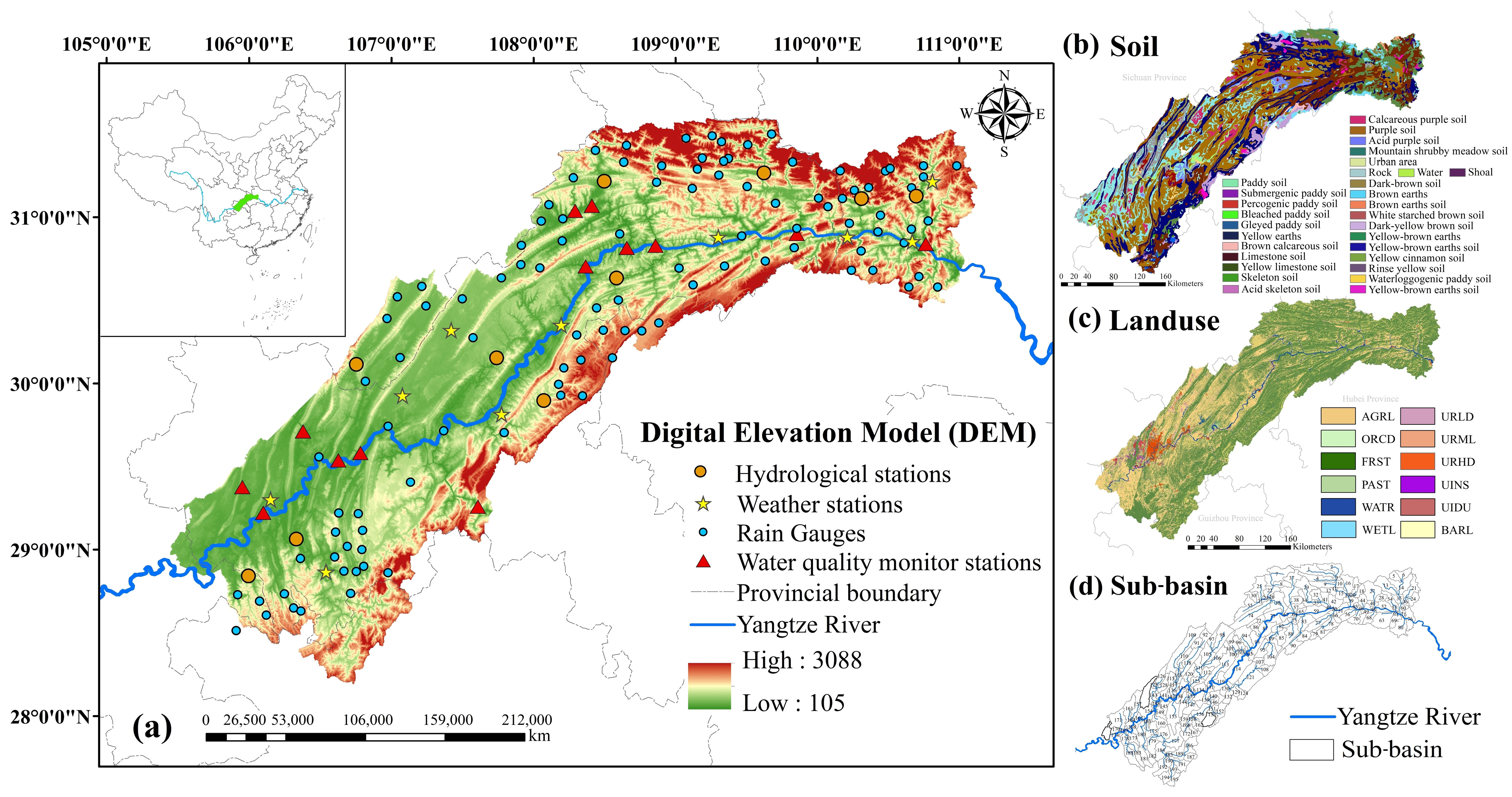
2.1. Study Area

The Yangtze River, which has a watershed area of 1,810,000 km² with a population of approximately 450 million people, is the third largest river in the world with complicated hydroclimatic conditions [13,22,25]. The Three Gorges Dam Project is one of the biggest hydropower complex projects in the world, which was completed in 2009 and forms the biggest reservoir in China [13,27]. The TGRA is situated in the middle reaches of the Yangtze River (28°28′–31°44′ N, 105°49′–111°39′ E) and involves a total of 26 districts and counties of the Chongqing City and Hubei Province. The study area covers the land surface of TGRA, and the total watershed area is about 64,000 km². Under the influence of a subtropical warm monsoon climate with distinctive basin climate features, rainfall is abundant, and rainstorm events occur frequently in the basin. The average annual temperature is equal to 20 °C, and annual precipitation is between 1000 and 1200 mm from 1961 to 2016, while rainfall is uneven throughout the years, with over 80% of precipitation falling in May–September [13,27]. Figure 1 shows the location, soil types, and land use map of the study area. The terrain of the entire watershed is undulating, with surface elevation ranging between 70 m and 3,105 m above sea level. The mountain area is the largest and accounts for more than 70%, followed by thills which accounts for about 20%, and the plain area is the smallest. According to the role and characteristics of land, land use types could be divided into different categories, and the largest area is agricultural land (28%), followed by forest and grassland. The soil types include purple soil, paddy soil, yellow-brown soil, lime soil, and so on. The purple soil, which is fertile and weak in erosion resistance, is the most widely distributed in the basin, accounting for about 36.8% of the total land area.

2.2. Methods of Analysis

2.2.1. Mann–Kendall Test

The Mann–Kendall (MK) test is a nonparametric statistical test that is generally used in the long time-series trend analysis of climate data, which has the advantage of a wide application range, simple calculation, and high accuracy [31,32,33]. The method does not need to hypothesize the statistical distribution of the samples in advance, which maintains higher reliability than other parametric methods. In addition, due to the low requirements for the data continuity of this method, it can be used to accurately describe the trend of long-term data. List the data in the order in which they were collected over time x₁, x₂, …, x_n, which denote the measurements obtained at times 1, 2, …, n, respectively. The MK test is based on the statistic S:

$$S={\displaystyle \sum _{i=1}^{n-1}{\displaystyle \sum _{j=i+1}^n\mathrm{sgn}(x_j-x_i)}}$$

(1)

where x₁, x₂, x₃, …, x_n are the observations listed in the order it is collected, j > i; x_j and x_i are the time series values; and n is the length of the data set.

$$\mathrm{sgn}(x_j-x_i)=\left\{\begin{array}{l}+1\hspace{1em}\hspace{1em}\left(x_j-x_i>0\right)\\ 0\hspace{1em}\hspace{1em} \left(x_j-x_i=0\right)\\ -1\hspace{1em}\hspace{1em}\left(x_j-x_i<0\right)\end{array}\right.$$

(2)

The mean and variance of the S statistic are calculated using the following formula:

$$E\left(S\right)=0$$

(3)

$$Var(S)=\frac{[n(n-1)(2n-5)-{\displaystyle \sum t_m(m-1)(2m+5)}]}{18}$$

(4)

where t_m is the number of times of extent m; n is the length of the data set. Based on the above formula, the normalized test statistic Z:

$$Z=\left\{\begin{array}{l}\frac{S-1}{\sqrt{Var(S)}}\hspace{1em}\hspace{1em}(S>0)\\ 0\hspace{1em}\hspace{1em}\hspace{1em}(S=0)\\ \frac{S+1}{\sqrt{Var(S)}}\hspace{1em}\hspace{1em}(S<0)\end{array}\right.$$

(5)

where Z is the test statistics. For the mutation analysis, the rank statistic (S_k) can be expressed by the following formula:

$$S_k={\displaystyle \sum _{i=1}^k{r}_i}\hspace{1em}\hspace{1em}(k=2,3,...,n)$$

(6)

$$r_i=\left\{\begin{array}{l}1\hspace{1em}\hspace{1em}(x_j>x_i)\\ 0\hspace{1em}\hspace{1em}(x_j\le x_i)\end{array}\right.\hspace{1em}\hspace{1em}(j=1,2,...,i)$$

(7)

where S_k is the cumulative number of cases x_j > x_i. Define the statistical variables:

$$U{F}_k=\frac{[S_k-E(S_k)]}{\sqrt{Var(S_k)}}\hspace{1em}\hspace{1em}(k=1,2,...,n)$$

(8)

where UF_k is the sequential values of the statistic; E(S_k) is the mean value of S_k; and Var(S_k) is the variance value of S_k. The specific calculation formulas of the value are as follows:

$$E(S_k)=\frac{n(n-1)}{4}$$

(9)

$$Var(S_k)=\frac{n(n-1)(2n+5)}{72}$$

(10)

$$U{B}_k=-U{F}_k$$

(11)

Based on the calculated values, the trend of the time series can be further analyzed to clarify the mutation time and the mutation region of the series. In this study, UF_k was normally distributed, which formed the forward sequence curve, and the backward sequence UB_k was obtained in the same way but in a reverse data series. If the two curves intersect within the confidence interval, the intersection point is the moment of abrupt change in the time series. The significance level of the test is α = 0.05.

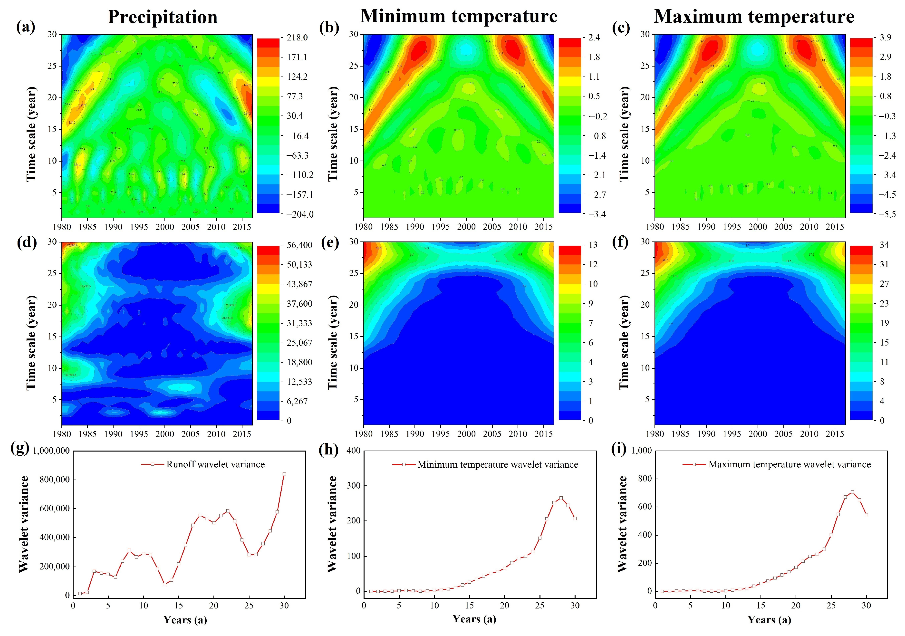
2.2.2. Wavelet Analysis

Wavelet, cross-wavelet, and coherence wavelet approaches were used to analyze the periodicity and correlation of the meteorological, hydrological and water quality elements. Wavelet analysis is developed based on the short-time Fourier transform. Compared with the Fourier analysis, wavelet analysis can not only determine the spectral characteristics of the signal in the time domain but also reflect local time spectral characteristics with a better resolution. The method used in this study was Morlet wavelet analysis, with the multi-resolution function, which is suitable for the periodic analysis of climate change processes based on long-time series meteorological data [33,34]. Morlet wavelet is the complex wavelet, and the function expression is:

$$\phi (t)=e^{i{\omega }_{0}t}{e}^{-t^2/2}$$

(12)

where i is an imaginary number; ω₀ is the wavelet central frequency. The calculation methods of wavelet transform, wavelet coefficient, and wavelet variance are as follows:

$$W_f(a,b)={\left|a\right|}^{-1/2}\Delta t{\displaystyle \sum _{k=1}^{N}f(k\Delta t)\phi }(\frac{k\Delta t-b}{a})$$

(13)

$$W_f(a,b)={\left|a\right|}^{-1/2}{\displaystyle \sum _{k=1}^{N}f(k)}\phi \cdot e^{ict}\cdot e^{-t/2}$$

(14)

$$Var(a)={{\displaystyle \underset{-\infty }{\overset{+\infty }{\int }}\left|W_f(a,b)\right|}}^{2}db$$

(15)

where a is the contraction-expansion factor; b is the time parameter; W_f(a,b) is the Morlet wavelet transform coefficient; Var(a) is the variance; c is the constant with the value of 6.2.

The cross-wavelet spectrum of sequences and degree of coherence of wavelet transform can be defined as:

$$W_n^{XY}(s)=W_n^X(s)W_n^{Y*}(s)$$

(16)

$$R_n^2(s)=\frac{{\left|S\left(s^{-1}{W}_n^{XY}(s)\right)\right|}^2}{S\left(s^{-1}{\left|W_n^X(s)\right|}^2\right)S\left(s^{-1}{\left|W_n^Y(s)\right|}^2\right)}$$

(17)

where $W_n^{XY}(s)$ is the wavelet cross spectrum; $W_n^X(s)$ and $W_n^Y(s)$ are the wavelet transform coefficients; $W_n^{Y*}(s)$ is the complex conjugate of $W_n^Y(s)$; s is the scale factor; and S is the smoothing operator.

2.2.3. Moving Average Analysis

Moving average is a common method used in trend fitting, and the average value of the different subsets can be used to show the trend of data change. For a long time series of data, the new series is obtained by adjusting the size of the sliding window to calculate the average of different time subsets, which makes the time variation trend of the original series more obvious and better reflects the changing trend. The appropriate sliding length k can average the high-frequency oscillation of the original sequence, though not too much:

$$y=\frac{1}{k}{\displaystyle \sum _{i=0}^{n-1}{x}_{k-i}}$$

(18)

where k is the appropriate sliding length; n is the length of the data set.

2.2.4. Anomaly Analysis

Anomaly analysis is a statistical method that indicates the deviation of data variables from normal conditions, which is often used in climate change studies. The difference between x_i and the multi-year average x_a is the anomaly value. In the analysis of the climate change trend, the climate data sequence can be transformed into a sequence with an average value of 0 after anomaly processing, which makes the calculation result more intuitive:

$$x_i={\displaystyle \sum _{i=1}^t(x_i-x_a)},\hspace{1em}t=1,2,3,\cdots ,n$$

(19)

$$x_a=\frac{1}{n}{\displaystyle \sum _{i=1}^n{x}_i}$$

(20)

where x_i is the values of meteorological elements at time i; x_a is the average annual value; n is the length of the data set; and t is the time series.

2.2.5. Spatial Interpolation

The Ordinary Kriging method was used to represent the evolution of the spatial distribution of meteorological elements in the TGRA. Kriging interpolation, also known as spatial local interpolation, considers both the spatial relativity of variables and the interrelationship between data point locations and is effective in spatial data interpolation. The Ordinary Kriging interpolation assumes that the properties of space are uniform and uses the weight associated with the measurement points (λ_i) to produce a predicted value of the unknown point. The general form of the equation can be written as:

$$Z^{*}(x_0)={\displaystyle \sum _{i=1}^n{\lambda }_i}Z(x_i)$$

(21)

where Z*(x₀) is the predicted value of the unknown points; Z(x_i) is the value of the known points; λ_i is the weight used in the calculation; and n is the number of observed values.

2.3. Hydrological Model

The SWAT model, a physically based distributed hydrological model with high precision, was developed by the USDA Agricultural Research Service and is suitable for watershed-scale water environmental simulation [18,35]. Based on the spatial data of the Geographical Information System (GIS) and Remote Sensing (RS), the SWAT model can accurately simulate complex water cycle processes in large-scale basins, such as runoff, sediment, solid–liquid distribution, erosion, groundwater, evapotranspiration, nutrient loss (nitrogen, phosphorus), heavy metals, and so on [20,35]. The SWAT model has the advantage of high operational efficiency and continuous time simulations. In the SWAT model, the river basins are usually divided into several sub-basins, which reduce the influence of various factors on the simulation accuracy in the watershed water cycle simulation. Afterward, the watershed is further divided into the hydrological response units (HRUs), which are the smallest discrete units of account and contain uniform land use, management practices, and soil property information [13,18]. The runoff and pollutants generated via surface and subsurface pathways were input to the stream network at the respective sub-watershed outlet [13,20].

2.3.1. Data Source

The specific sources, accuracy, and format of the input data required by the SWAT model are shown in the Supplementary Materials (Table S1). The Digital Elevation Model (DEM), land use, soil type, and other data were provided by the different professional institutions, and the data accuracy met the simulation requirements of the TGRA. In previous studies, the SWAT model, when established with the same precision data, could accurately simulate the water environment process in a large-scale watershed [13,22]. In the study area, there were 22 weather stations and 113 rain stations, which could fully reflect the spatial distribution of the meteorological elements in the study area. The daily meteorological data of the stations were collected from the National Data Center for Meteorological Sciences and Hydrologic Statistical Yearbooks. The watershed hydrology and water quality data were collected from the Hydrology Bureau of Yangtze River Water Resources Commission. The 3710 specific point source emissions data of the study area were collected from the Chongqing Academy of Environmental Science, and the non-point source emission was calculated by the SWAT model.

2.3.2. Model Setup

The SWAT model can automatically generate the basin boundary and sub-basin layers based on accurate DEM data. Therefore, the watershed was divided into 187 sub-basins using a threshold drainage area of 2000 ha, which was successfully applied in previous watershed simulation studies [13,22]. Based on the heterogeneity of topography, land use, and soil type, 183 sub-basins provided 4282 HRUs. The land use/cover in the current year of 2018 and the meteorological data with a period of 1980–2018 were used as the input conditions for modeling. The SWAT model was calculated for 38 years, while the period could be divided into two parts: the warm-up period (1980–1981) and the simulation period (1882–2018).

2.3.3. Model Calibration and Validation

The calibration and verification of the SWAT model were conducted using the GLUE methodology in the study, which took input uncertainty, structural uncertainty, parameter uncertainty, and response uncertainty into account. The details and specific steps of the model evaluation are presented by Shi et al. (2017) and Chen et al. (2019) [13,22]. The model was calibrated, first in the order of runoff and then water quality. It was impossible to adjust all parameters during the calibration process, while the most sensitive parameters which affected the simulation of runoff, TN, and TP loads were selected for calibration. The selected parameters were basically consistent with the previous SWAT model studies [13,35]. The sensitivity of the model parameters could be divided into four grades: high-grade, middle-grade, primary-grade, and low-grade, and the details are shown in the Supplementary Materials (Table S2).

The model performance was evaluated by the coefficient of determination (R²) and the Nash Sutcliffe efficiency (E_NS), which are widely used to evaluate the model simulation [36,37,38]. R² indicates the strength of the covariance between the model simulation data and the monitoring data, with a value range from 0 to 1. The higher the R² value was, the better the model simulation effect; and the acceptable range of the simulation accuracy was greater than 0.5. E_NS ranged from 1 to negative infinity. For the value of E_NS, when E_NS was higher than 0, the model simulation effect met the application requirements, while the reverse indicated that the model simulation accuracy was insufficient:

$$R^2=\frac{{\left[{\displaystyle \sum _{i=1}^n\left(Q_{m,i}-{\overline{Q}}_m\right)\left(Q_{s,i}-{\overline{Q}}_s\right)}\right]}^2}{{\displaystyle \sum _{i=1}^n{\left(Q_{m,i}-{\overline{Q}}_m\right)}^2{\displaystyle \sum _{i=1}^n{\left(Q_{s,i}-{\overline{Q}}_s\right)}^2}}}$$

(22)

$$E_{NS}=1-\frac{{\displaystyle \sum _{i=1}^n{\left(Q_{m,i}-Q_{s,i}\right)}^2}}{{\displaystyle \sum _{i=1}^n{\left(Q_{m,i}-{\overline{Q}}_m\right)}^2}}$$

(23)

where Q is the runoff or water quality concentration; $\overline{Q}$ is the average of all observations; m is the measured values; and s is the simulated values.

2.4. Correlation Analysis

The Pearson correlation coefficient is widely used to detect the correlation between two different variables. The Pearson correlation coefficient ranged from −1 to 1, indicating that the correlation between the variables ranged from a completely unrelated to a completely positive correlation. In this study, the correlations between climate change, extreme climate indicators, runoff, TN, and TP loads were analyzed using this method. The formula is as follows:

$$P_{x,y}=\frac{{\displaystyle \sum \left(x-x^{\prime }\right)}{\displaystyle \sum \left(y-y^{\prime }\right)}}{\sqrt{{\left(x-x^{\prime }\right)}^2}\sqrt{{\left(y-y^{\prime }\right)}^2}}$$

(24)

where P_x,y is the correlation coefficient; x′ is the average value of variable x; and y′ is the average value of variable y.

3. Results and Discussion

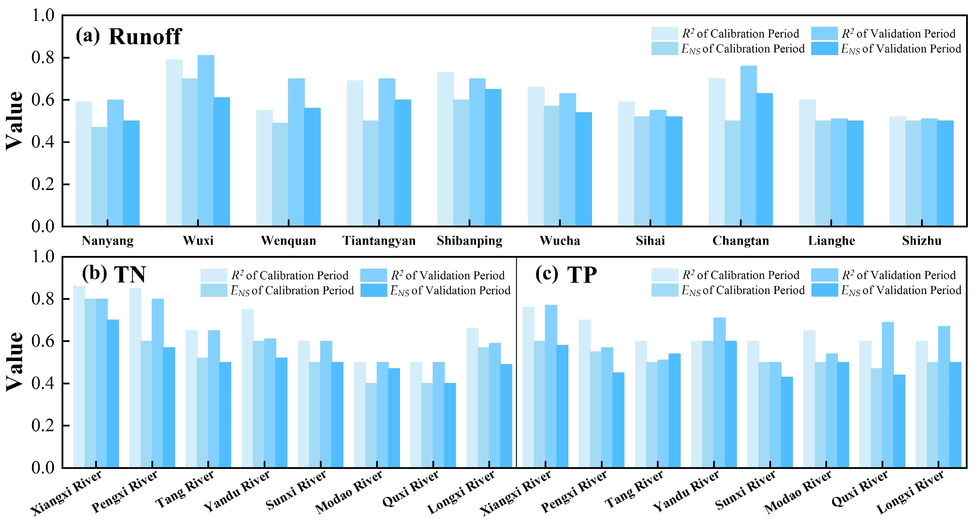
3.1. Calibration and Validation Results

Daily runoff and water quality results during the period of 2003–2007 were utilized for calibration and were validated over the period from 2008 to 2012. The monitoring runoff data were provided by 10 hydrological stations, and the monitoring water quality data were obtained by the water quality monitoring stations of the study area. The locations of the monitoring stations are shown in Figure 1. The major parameters, which are most sensitive to the watershed water cycle processes and the transport and transformation of nutrients, were employed for calibration purposes. The results of the principal parameters are shown in

Table 1. The sensitivity value, sensitivity level, and sensitivity rank of principal parameters which related to runoff, total nitrogen (TN), and total phosphorus (TP) loads.

	Parameter	Parameter Definition	Sensitivity Value	Level	Rank
Runoff	CN2	Moisture condition II curve number	2.99	IV	1
	CH_K2	Effective hydraulic conductivity	2.67	IV	2
	SOL_AWC	Soil available moisture content	2.28	IV	3
	ALPHA_BF	Baseflow alpha factor	1.97	III	4
	ESCO	Soil evaporation compensation factor	1.91	III	5
	GW_DELAY	Groundwater delay	1.85	III	6
	GWQMN	Threshold depth of water in the shallow aquifer required for return flow to occur	0.97	III	7
	REVAPMN	Threshold depth of water in the shallow aquifer for evaporation to occur	0.81	III	8
	CH_N2	Manning’s value for main channel	0.60	III	9
	SOL_BD	Soil moisture bulk density	0.30	III	10
TN	RCN	Concentration of nitrogen in rainfall	3.31	IV	1
	SOL_ORGN	Initial organic N concentration in the soil layer	1.58	IV	2
	SDNCO	Denitrification threshold water content	0.87	III	3
	BC1	Rate constant for biological oxidation of NH3	0.82	III	4
	BC2	Rate constant for biological oxidation of NO2 to NO3	0.28	III	5
TP	FILTERW	Width of the edge of field filter strip	2.71	IV	1
	SOL_ORGP	initial humic organic phosphorus in soil layer	2.13	IV	2
	PHOSKD	Phosphorus soil partitioning coefficient	1.08	IV	3
	BC4	Phosphorus soil partitioning coefficient	0.88	III	4
	PSP	Phosphorus sorption coefficient	0.76	III	5

. The results showed that CN2 (Moisture condition II curve number) was most sensitive to runoff modeling and was followed by CH_K2 (Effective hydraulic conductivity) and SOL_AWC (Soil available moisture content). In the process of TN and TP simulation, RCN (Concentration of nitrogen in rainfall) and FILTERW (Width of the edge of field filter strip) showed the strongest sensitivity, which reached 3.31 and 2.71, respectively. A detailed analysis of the parametric sensitivity and uncertainty of the study area was available in our previous work [13,22]. Compared with the previous studies, the sensitive parameters of the watershed water environment simulation were similar.

Figure 2 illustrates an agreement between the simulated and monitored results of runoff, TN, and TP. Regarding the results of runoff, the R² range of the calibration period was 0.52–0.79, and the R² range of the verification period was 0.55–0.81, while the corresponding E_NS had a range from 0.47 to 0.70 and 0.50 to 0.65, respectively. During the calibration period, the R² of TN simulation results ranged from 0.50 to 0.86, and the value range of E_NS was 0.42–0.63, while the R² and E_NS value of TP simulation ranged from 0.58 to 0.76 and 0.47 to 0.76, respectively. In the validation period, the minimum R² value of TN simulation was 0.52, and the maximum value was 0.81, while the range of E_NS was 0.40–0.69. Meanwhile, the R² of TP ranged from 0.52 to 0.77, and the E_NS values were in the range of 0.43–0.61. The simulation accuracy of the SWAT model for runoff, TN, and TP loads could meet the requirement of the accuracy of the watershed water environment simulation.

It was expected that a slightly weaker performance for the water quality simulation would be observed compared to that for runoff. The main reason for this was that the transport and transformation processes of the watershed pollutants were more complex than those that the runoff and the changes in hydrodynamic conditions and underlying surface characteristics would affect the simulation of the complex pollutant transport processes. Compared with the previous simulation research, the SWAT model adopted in the study had an acceptable simulation accuracy, which met the requirements of the simulation [13,22,35].

3.2. Spatial and Temporal Distribution of Climate Change

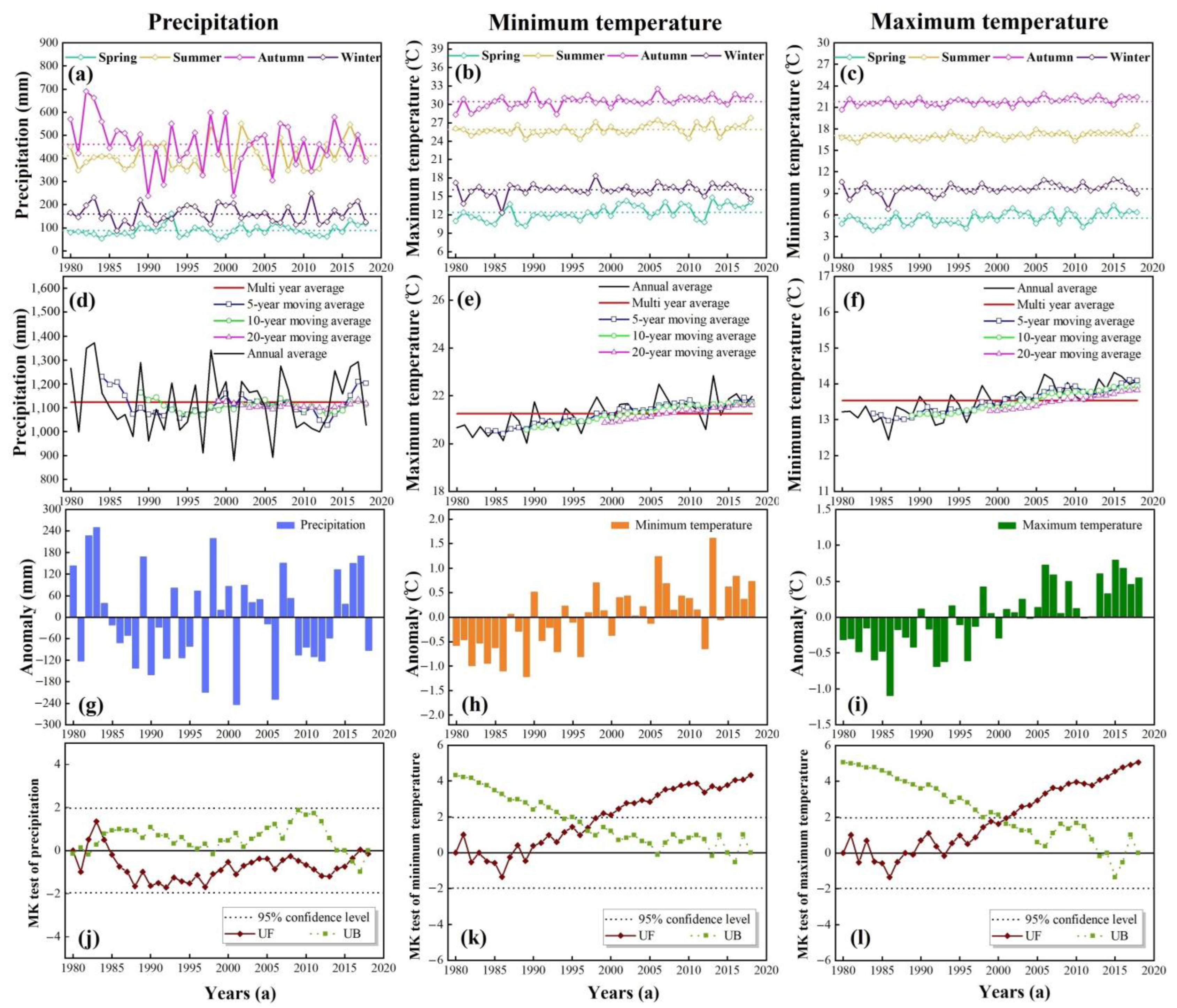
3.2.1. Temporal Distribution

In order to better investigate the characteristics of the regional climate change of TGRA, the precipitation, minimum temperatures and maximum temperatures, along with the long time series from 1980 to 2018, were analyzed. The trend test results of the three variables, are shown in Figure 3. The seasonal precipitation decreased in the following order autumn (461.31 mm) > summer (412.42 mm) > winter (159.97 mm) > spring (88.83 mm). Under the increasing influence of climate change, the variability of the inter-annual and inner-annual value of the regional climate gradually strengthened in the TGRA, and the uncertainty of precipitation increased and fluctuated greatly [4,7]. The seasonal variation trends in temperature were similar to that of precipitation, which were highest in autumn followed by summer. The inter-annual variation in the seasonal average temperature was smaller, especially in summer and autumn.

The moving averages with the different yearly scales of precipitation and minimum and maximum temperatures were selected to reveal the frequency changes in climate variables for the historical periods. The annual precipitation of the study area was 1121.92 mm, which showed a large fluctuation from 1980 to 2018, while the lowest precipitation value, 878.46 mm, occurred in 2001. Compared with the other large river basins with a complex ecological environment, such as the Yellow River, Songhua River, and Hanjiang River, the Yangtze River basin had higher annual precipitation [14,16,21]. As shown in Figure 3, there were two obvious fluctuations in precipitation from 1980 to 2018, and the dividing year was 2000. Over the two periods, the precipitation obviously showed a trend of first decreasing and then increasing. From the perspective of a multi-time scale, the average annual values of the minimum and maximum temperature were 13.53 °C and 21.23 °C. The maximum and minimum temperatures showed an increasing trend, with linear change rates of 0.38 °C/10a and 0.29 °C/10a, respectively. This change was mainly influenced by global warming, with the IPCC’s Fifth Assessment Report stating that the global average land and sea temperatures increased by 0.89 °C during 1901–2012 [39,40]. Previous studies have also shown that the global temperature showed a gradual upward trend since the 2000s, which has required more attention [39].

The percentage of the anomaly can be used as an important method to characterize the excess (deficit) of precipitation and minimum and maximum temperature over the multi-year average for a certain period. The results of the annual precipitation anomaly analysis showed that there was no obvious trend of precipitation, which showed a strong periodic fluctuation. Larger precipitations were recorded in 1982, 1983, and 1998, which coincided with the records of a major flood disaster that occurred in the Yangtze River Basin. The temperature anomaly results showed that the temperature had a significant rising trend. There were three temperature periods during the study period: the cooling period (1980 to 1990), the warming period (1990 to 2000), and the accelerated warming period (2000 to 2018).

Figure 3 shows the MK test of precipitation and minimum and maximum temperature in the TGRA. In this study, the significance level of the test was α = 0.05. The phenomenon of the precipitation was quite different from that of temperature. It can be summarized by stating that the precipitation change was not significant, and there was no obvious mutation point, which is consistent with the analysis above. The UF and UB curves of precipitation had multiple points of intersection in the confidence interval, which were located between the two critical lines. The UF value was negative from 1985 to 2016, indicating that the precipitation of the study area presented an overall decreasing trend of fluctuation after 1985. It showed an obvious trend in both minimum and maximum temperatures over the past few decades. The UF curves showed that UF values were mostly negative before 1990, while all of them were positive after 1990, indicating that the minimum and maximum temperatures changed from low to high. The UF value of temperature exceeded the upper confidence limit, indicating that the abrupt points of the minimum and maximum temperature were 1998 and 2001, while the temperature presented an obvious increasing trend after the abrupt point.

Wavelet analysis was applied to examine the periodic variation in the annual precipitation and minimum and maximum temperature (Figure 4). Positive areas of the real part of the Morlet wavelet analysis indicated high annual precipitation and temperature, while negative areas indicated the contrary. The contours of precipitation and temperature were relatively dense in the study period and indicated that the change was drastic while the fluctuation range was large. Combining the results of the wavelet variance test and the contour map of the real part of wavelet coefficients, the oscillation period of precipitation with the densest and the most significant contour value center was about 22 a, and the oscillation period of temperature was 28 a. Previous studies have also shown that the Wujiang River, an important tributary of the Yangtze River, and the main principle cycle of annual precipitation was 29 years, which was similar to the periodic period of the study [41].

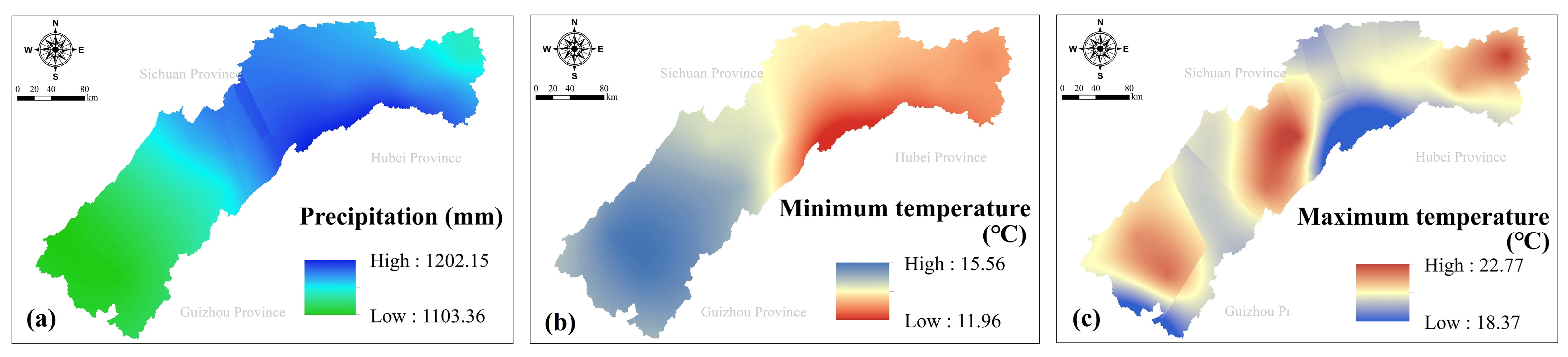
3.2.2. Spatial Distribution

The spatial distribution of precipitation and minimum and maximum temperature from 1980 to 2018 is depicted in Figure 5. For the most recent past period, precipitation presented a trend less-more-less from west to east, as lower elevations were commonly associated with less precipitation. In addition to the influence of atmospheric circulation, the spatial distribution of precipitation was also affected by the local topography and altitude [13,22]. Due to the extensive mountainous area and rugged terrain in the TGRA, the precipitation was abundant in the reservoir area, but the spatial distribution was not uniform [13,24]. High temperature centers appeared in the urban area of Chongqing city, Zhongxian city, and Xingshan city, with stronger economic development. Compared with the land use types distribution above (Figure 1c), it could be found that the area with a higher vegetation coverage and lower human activity intensities had a lower temperature [24]. The temperature distribution of the study area was highly susceptible to the degree of human activities (carbon emissions) and vegetation coverage, thus the temperature in the large urban area with high human activities was generally higher than in the area with high vegetation coverage [42,43,44,45].

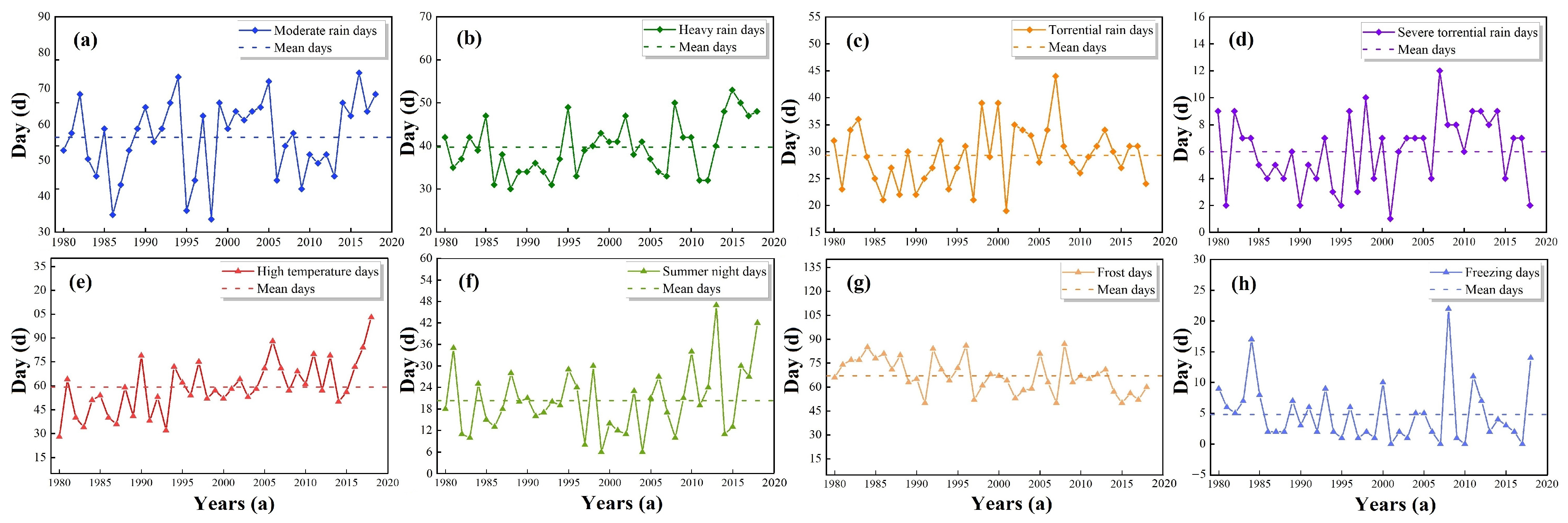
3.2.3. Extreme Weather

As extreme climate events occur frequently, the inter-annual characteristics of climate extremes have changed substantially. The inter-annual variation characteristics of extreme climate events from 1980 to 2018 are shown in Figure 6, and the extreme weather indicators are shown in Table S3. The extreme precipitation days showed an increasing trend between 1980 and 2018, indicating that the extreme precipitation weather increased prominently under the background of global climate change [46]. Meanwhile, the extreme temperature days in the study area increased gradually. The United Nations has stated that extreme weather events have increased more than fivefold over the past few decades, with a significant increase in growth trends in just over two decades. The summer night days and high-temperature days showed an increasing trend, while the frost days and freezing days showed a decreasing trend. While climate change does not directly cause heavy rainfall or drought, it makes these naturally occurring events more intense or severe. The scenario that increased extreme weather events caused by global climate change could lead to deeper changes in the watershed water cycle and has been supported by several previous modeling prediction studies [4,15,46].

3.3. Spatial and Temporal Distribution of Runoff, TN and TP Loads

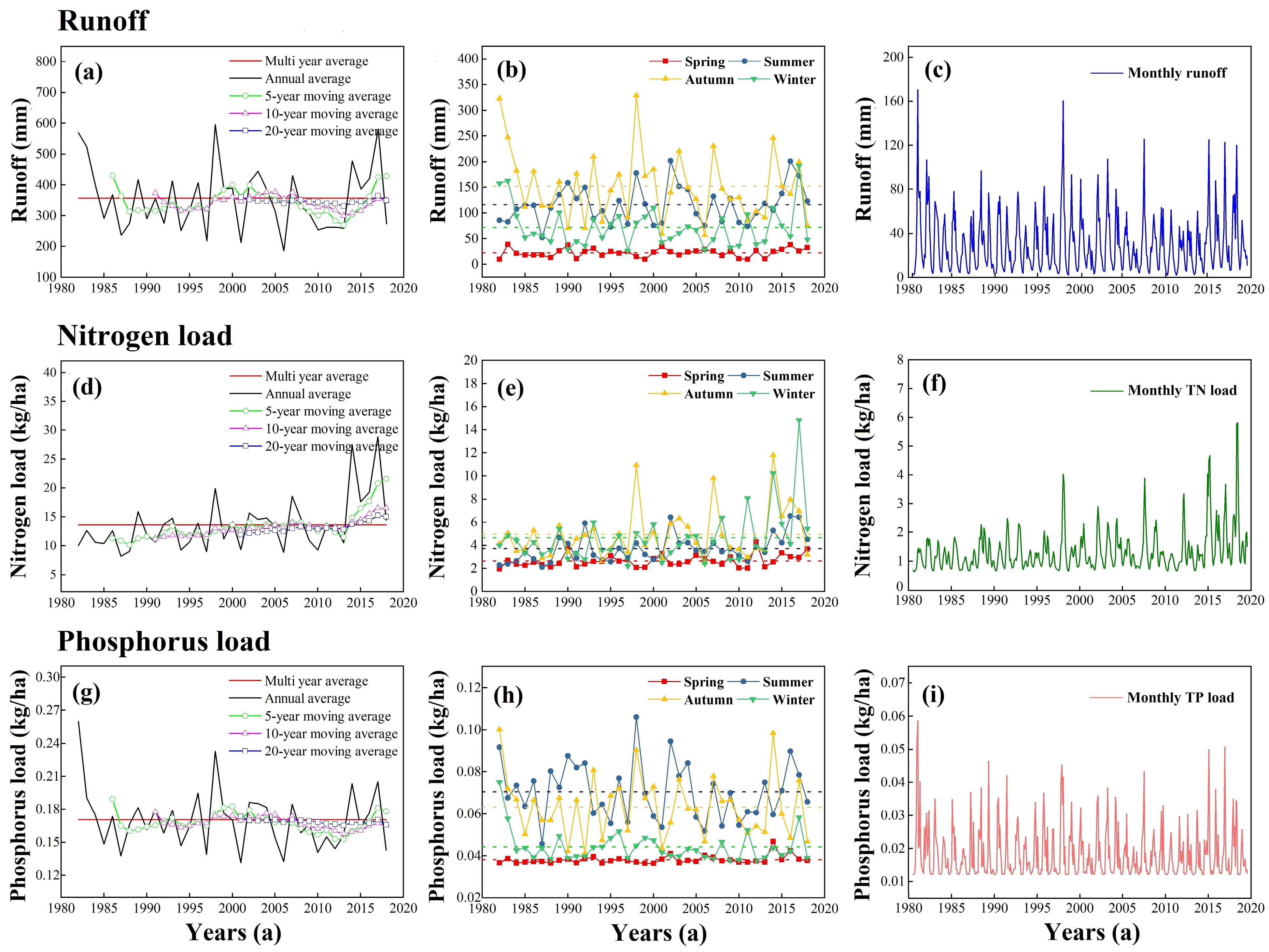
3.3.1. Temporal Distribution

The temporal trends of runoff, TN, and TP loads in the study area under climate change are shown in Figure 7. The average annual runoff for the past 40 years was 356.17 mm, and the average annual TN, and TP were 13.61 kg/ha and 0.17 kg/ha, respectively. The average annual value of runoff, TN and TP loads showed a decreasing trend followed by an increasing trend and fluctuated violently within the short period, possibly due to the same severe interannual fluctuation of precipitation [10,12]. A monthly variation in runoff showed a fluctuation of cyclical variation, specifically from June to August. The highest monthly runoff was in July 1982, which reached 170.49 mm, and the lowest monthly runoff occurred in July 2006, with a value of 2.17 mm. The monthly variation in TN and TP loads also showed cyclical fluctuations, such as runoff, as evidenced by the peaks from June to August.

Figure 7 shows the trends of runoff, TN, and TP loads in different seasons. The multi-year seasonal value of runoff showed a trend of autumn (151.55 mm) > summer (115.91 mm) > winter (71.73 mm) > spring (22.34 mm), and the runoff fluctuated widely in autumn, with the highest value of 328.79 mm in 1998 and the lowest value of 56.26 mm in 2006. The result indicates that the intra-annual distribution of meteorological elements became more and more uneven due to climate change, leading to profound changes in water environment elements, especially in terms of runoff [47,48]. The multi-year seasonal average value of TN was the following: autumn (4.93 kg/ha) > winter (4.64 kg/ha) > summer (3.71 kg/ha) > spring (2.65 kg/ha), but the value of TP in autumn was lower than in summer. Compared with runoff, the seasonal average of TN and TP simulations showed a lower inter-annual fluctuation. Under the influence of climate change, especially after the operation of the Three Gorges Dam Project, the local microclimate of the basin might lead to an obvious decrease in the differences between runoff and TP across seasons. The seasonal fluctuation trend of TN showed an increasing trend during the study period, which was possibly due to an increase in the extreme precipitation conditions caused by climate change, which increased the probability of higher nutrient loads due to surface erosion [49,50].

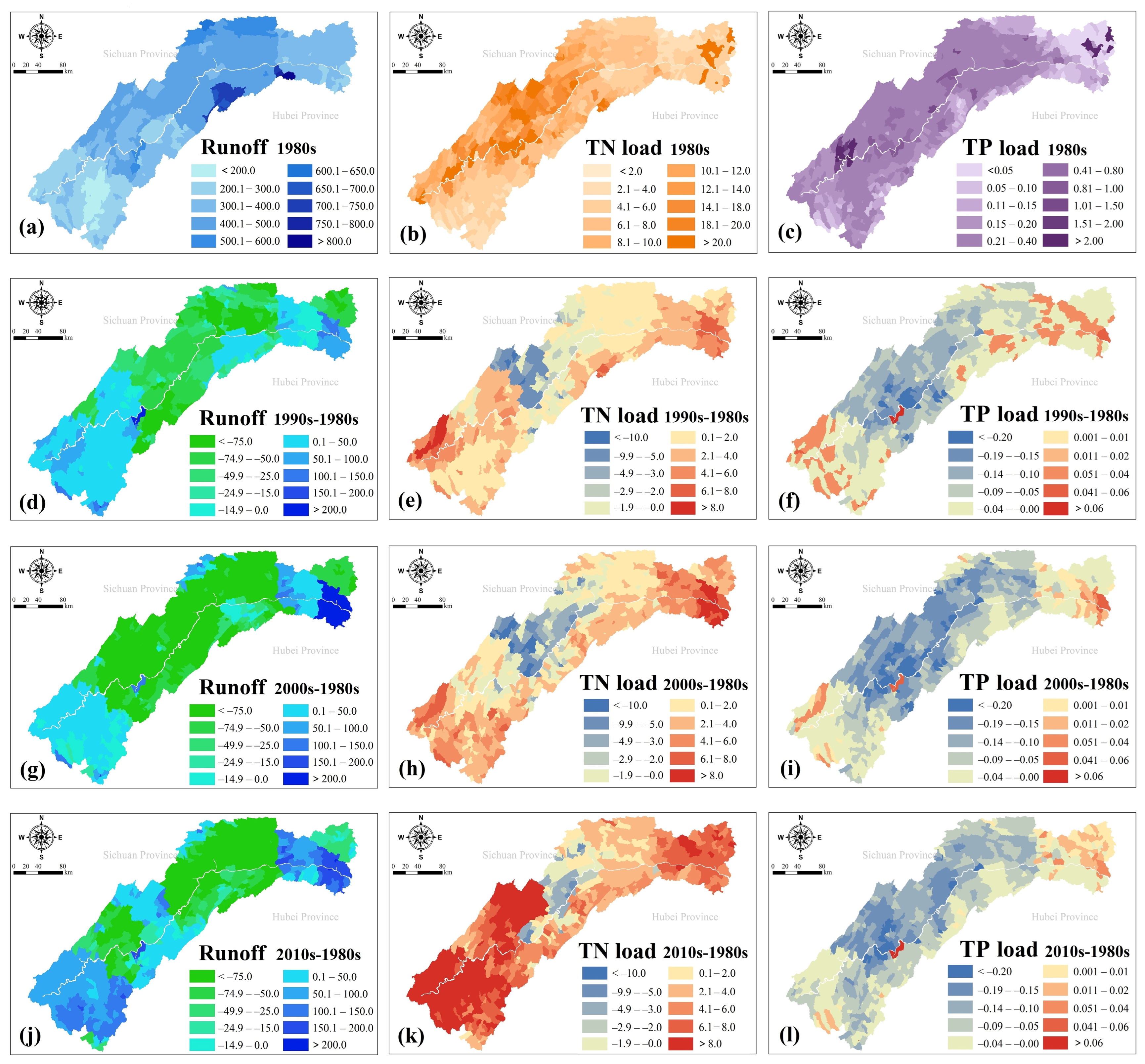
3.3.2. Spatial Distribution

The impacts of climate change on the spatial distribution of runoff, TN, and TP loads are presented in Figure 8, while Figure 8a–c are spatial distributions under 1980s meteorological conditions, and Figure 8d–l are the difference between the 1990s, the 2000s, the 2010s, and the 1980s, respectively. The hydrological processes changed significantly at different spatial scales during the last 40 years. Under the meteorological conditions in the 1980s, higher runoff areas were mainly distributed in the middle and head reservoir areas, where the average values were 429.87 mm and 404.23 mm, and the lower was in the tail area, which was only 270.11 mm. Compared with the 1980s, the runoff in the middle area of the reservoir decreased significantly in the 1990s, 2000s, and 2010s, while there was a significant increase in the head and tail area. In the large-scale watershed, the hydrological elements might appear to have opposite trends in the upstream and lowland areas, i.e., an increase in precipitation in the upstream area might result in a higher runoff while the downstream even showed a downward trend. Previous studies have shown such opposing trends in the Nile basin, which increased in the runoff upstream of the Blue and White Nile and decreased downstream [2,51,52,53]. Under the meteorological conditions in the 1980s, the area with a higher TN load was distributed in the middle area of the reservoir, with an average TN value of 11.01 kg/ha, while the lower TN occurred in the head and tail area. The spatial distribution of TP was similar to that of TN in the 1980s. Compared with the 1980s, the TN showed an increasing trend, while the TP showed an opposite trend during the study period. In addition, climate change in the 2000s had the most significant impact on runoff, TN, and TP loads.

3.4. Response Relation

3.4.1. Climate Change Impact

The correlation analysis results were used to characterize the correlation between climate indicators, runoff, TN, and TP loads, while temperature had little correlation with runoff, TN, and TP. The Pearson correlation coefficient between the precipitation and runoff reached 0.91 (Figure 9), and the significance level is less than 0.001, indicating that precipitation was an important factor affecting the inter-annual variation of runoff during the study period. From the wavelet spectrum, the correlation of precipitation and runoff optimally explains runoff variations (Figure 10). Annual precipitation and annual runoff showed a 3–5-years high energy resonance zone around 1995 and 2003. The coherence wavelet presented the same phases as those observed in the cross-wavelet, with a high level of correlation (0.80–1.00). The precipitation had a significant impact on rainfall during the study period. These results were consistent with several previous studies, while climate change had a great impact on runoff by affecting the precipitation and evaporation of the large river basin [54,55,56]. The Pearson correlation coefficient between TN and precipitation was only 0.60, which indicated that precipitation had a lower influence on TN, while the correlation was not significant. In addition to the slope erosion caused by rainfall runoff, industrial point source emissions and domestic sewage emissions caused by human activities are more important pollution sources of TN, especially the larger watershed with a high population density [25,57,58,59]. Compared with TN, the correlation value between precipitation and TP (0.81) was higher. TP mainly comes from soil erosion, and rainfall is the most direct factor leading to soil erosion [60,61,62]. The wavelet coherency results suggested that the precipitation had lower correlations with TN and TP loads than that of runoff, with the range of 0.4–0.9 for TN load and 0.6–0.9 for TP load, respectively. With climate change, the variability in the water cycle was intensified, which may bring extreme rainfall events and associated flooding, as well as higher water environment pollution [24,46]. It is necessary for the national government and various departments to formulate targeted adaptation policies to achieve regional sustainable water resources management.

3.4.2. Extreme Weather Impact

The correlation results between runoff, TN and TP loads, and extreme climate indicators are shown in

Table 2. Correlation between runoff, TN and TP loads, and extreme climate indicators.

	Indicator	Runoff	TN	TP
P100	Severe torrential rain days	0.54	0.44	0.55
P50	Torrential rain days	0.57	0.40	0.52
P25	Heavy rain days	0.19	0.35	0.03
P10	Moderate rain days	0.07	0.22	0.02
FD	Frost days	−0.13	−0.40	−0.05
SND	Summer night days	−0.17	−0.01	−0.16
HTD	High temperature days	−0.37	0.08	−0.37
FRD	Freezing days	0.01	−0.02	−0.04

. Extreme precipitation indicators showed positive correlations with runoff, TN, and TP loads and had a large effect. Severe torrential rain days (P100) and torrential rain days (P50) were highly correlated with runoff and with the correlation coefficients of 0.57 and 0.54, respectively. Previous studies indicated that the increase in the precipitation of a large watershed, especially in summer, a season with frequent rainstorms, would lead to a significant increase in watershed runoff and even lead to the occurrence of floods [6,63,64]. The extreme precipitation indicators showed a positive correlation with TN and TP, but correlations were lower than runoff. Previous studies have shown that extreme precipitation events had a potentially large impact on water quality, especially in high-risk areas of non-point source pollution [24]. In particular, the extreme precipitation events after successive droughts could wash many mineral elements, nutrients, pathogens, and other pollutants into the river and lead to more pollution in water bodies; excessive amounts of TN and TP could increase the risk of water eutrophication and result in a high probability of water pollution events [65,66,67].

4. Conclusions

Under the influence of increasing regional climate change, the complexity and uncertainty of the watershed environment in the TGRA are increasingly evident. Based on the practical requirements of integrated watershed environment management, the analysis of the corresponding relationship between climate change and the watershed environment is an important technical support for the development of relevant adaptation measures. In this paper, the temporal and spatial variation characteristics of climatic changes were analyzed based on meteorological monitoring data from 1980 to 2018 in the TGRA. The evolution of complex processes in the watershed environment was investigated using the SWAT model.

• The inter-annual variation in precipitation fluctuated greatly during the study period, and there was no abrupt change point. The temperature showed an increasing trend; the increasing rates of the maximum and minimum temperature were 0.38 °C/10a and 0.29 °C/10a, respectively. The precipitation presented a spatial distribution trend of less-more-less from west to east, while high temperatures mainly appeared in the urban area. Extreme precipitation events and extremely hot weather have increased during the past decades.
• The average annual value of runoff, TN, and TP loads showed a decreasing trend followed by an increasing trend and fluctuated violently within the short period. The runoff decreased significantly at the head and middle reservoir region, while it also showed an increasing trend at the tail reservoir area. Except for a few areas of the middle region, TN in most areas showed an increasing trend while TP decreased.
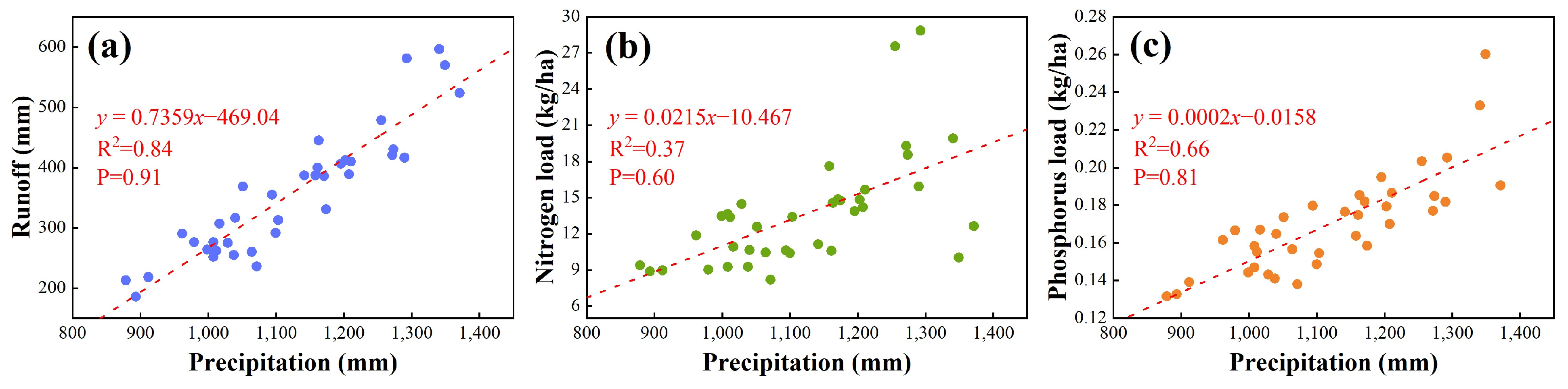
• Climate change and extreme precipitation events have had a significant impact on the runoff and TP load, while the impact on the TN load has increased significantly over the past 20 years. With climate change, variability in the water cycle has intensified, which may bring floods and greater pollution in the water environment. It is necessary for the national government and various departments to conduct more comprehensive assessments of climate change and its influence to support integrated water resources management.

References

1. Zhang, J.; Li, S.Y.; Dong, R.Z.; Jiang, C.S.; Ni, M.F. Influences of land use metrics at multi-spatial scales on seasonal water quality: A case study of river systems in the Three Gorges Reservoir Area, China. J. Clean Prod. 2018, 206, 76–85. [Google Scholar] [CrossRef]
2. Ye, X.C.; Zhang, Q.; Liu, J.; Li, X.H.; Xu, C.Y. Distinguishing the relative impacts of climate change and human activities on variation of streamflow in the Poyang Lake catchment, China. J. Hydrol. 2013, 494, 83–95. [Google Scholar] [CrossRef]
3. Sinha, E.; Michalak, A.M. Precipitation Dominates Interannual Variability of Riverine Nitrogen Loading across the Continental United States. Environ. Sci. Technol. 2016, 50, 12874–12884. [Google Scholar] [CrossRef] [PubMed]
4. Elsner, M.M.; Cuo, L.; Voisin, N.; Deems, J.S.; Hamlet, A.F.; Vano, J.A.; Mickelson, K.E.B.; Lee, S.Y.; Lettenmaier, D.P. Implications of 21st century climate change for the hydrology of Washington State. Clim. Chang. 2010, 102, 225–260. [Google Scholar] [CrossRef] [Green Version]
5. Steinman, B.A.; Abbott, M.B. Isotopic and hydrologic responses of small, closed lakes to climate variability: Hydroclimate reconstructions from lake sediment oxygen isotope records and mass balance models. Geochim. Cosmochim. Acta 2013, 105, 342–359. [Google Scholar] [CrossRef]
6. Milly, P.C.D.; Dunne, K.A.; Vecchia, A.V. Global pattern of trends in streamflow and water availability in a changing climate. Nature 2005, 438, 347–350. [Google Scholar] [CrossRef]
7. Marhaento, H.; Booij, M.J.; Hoekstra, A.Y. Hydrological response to future land-use change and climate change in a tropical catchment. Hydrolog. Sci. J. 2018, 63, 1368–1385. [Google Scholar] [CrossRef] [Green Version]
8. Archer, D.R.; Fowler, H.J. Spatial and temporal variations in precipitation in the Upper Indus Basin, global teleconnections, and hydrological implications. Hydrol. Earth Syst. Sc. 2004, 8, 47–61. [Google Scholar] [CrossRef] [Green Version]
9. Shrestha, S.; Bhatta, B.; Shrestha, M.; Shrestha, P.K. Integrated assessment of the climate and land use change impact on hydrology and water quality in the Songkhram River Basin, Thailand. Sci. Total Environ. 2018, 653, 1610–1622. [Google Scholar] [CrossRef]
10. Wang, X.; He, K.; Dong, Z. Effects of climate change and human activities on runoff in the Beichuan River Basin in the northeastern Tibetan Plateau, China. Catena 2019, 176, 81–93. [Google Scholar] [CrossRef]
11. Shahid, M.; Rahman, K.U. Identifying the Annual and Seasonal Trends of Hydrological and Climatic Variables in the Indus Basin Pakistan. J. Atmos. Sci. 2020, 57, 191–205. [Google Scholar] [CrossRef]
12. Hang, Y.F.; Guan, D.X.; Jin, C.J.; Wang, A.Z.; Wu, J.B.; Yuan, F.H. Analysis of impacts of climate variability and human activity on streamflow for a river basin in northeast China. J. Hydrol. 2011, 410, 239–247. [Google Scholar] [CrossRef]
13. Chen, X.M.; Xu, G.H.; Zhang, W.S.; Peng, H.; Xia, H.; Zhang, X.; Ke, Q.; Wan, J. Spatial Variation Pattern Analysis of Hydrologic Processes and Water Quality in Three Gorges Reservoir Area. Water 2020, 11, 2608. [Google Scholar] [CrossRef] [Green Version]
14. Zhou, F.; Xu, Y.; Chen, Y.; Xu, C.Y.; Gao, Y.; Du, J. Hydrological Response to Urbanization at Different Spatio-Temporal Scales Simulated by Coupling of CLUE-S and the SWAT Model in the Yangtze River Delta Region. J. Hydrol. 2013, 485, 113–125. [Google Scholar] [CrossRef]
15. Qian, S.S.; Kennen, J.G.; May, J.; Freeman, M.C.; Cuffney, T.F. Evaluating the impact of watershed development and climate change on stream ecosystems: A Bayesian network modeling approach. Water Res. 2021, 205, 117685. [Google Scholar] [CrossRef] [PubMed]
16. Wang, Y.; Zhang, W.; Zhao, Y.; Peng, H.; Shi, Y. Modelling water quality and quantity with the influence of inter-basin water diversion projects and cascade reservoirs in the Middle-lower Hanjiang River. J. Hydrol. 2016, 541, 1348–1362. [Google Scholar] [CrossRef]
17. Xu, X.; Wang, Y.C.; Kalcic, M.; Muenich, R.L.; Yang, Y.C.E.; Scavia, D. Evaluating the impact of climate change on fluvial flood risk in a mixed-use watershed. Environ. Modell. Softw. 2019, 122, 104031. [Google Scholar] [CrossRef]
18. Worku, G.; Teferi, E.; Bantider, A.; Dile, Y.T. Modelling hydrological processes under climate change scenarios in the Jemma sub-basin of upper Blue Nile Basin, Ethiopia. Clim. Risk Manag. 2021, 31, 100272. [Google Scholar] [CrossRef]
19. Debele, B.; Srinivasan, R.; Parlange, J.Y. Coupling upland watershed and downstream waterbody hydrodynamic and water quality models (SWAT and CE-QUALW2) for better water resources management in complex river basins. Environ. Model Assess. 2008, 13, 135–153. [Google Scholar] [CrossRef]
20. Wang, R.Y.; Yuan, Y.P.; Yen, H.; Grieneisen, M.; Arnold, J.; Wang, D.; Wang, C.Z.; Zhang, M.H. A review of pesticide fate and transport simulation at watershed level using SWAT: Current status and research concerns. Sci. Total Environ. 2019, 669, 512–526. [Google Scholar] [CrossRef]
21. Yuan, Z.; Yan, D.H.; Yang, Z.Y.; Xu, J.J.; Huo, J.J.; Zhou, Y.L.; Zhang, C. Attribution assessment and projection of natural runoff change in the Yellow River Basin of China. Mitig. Adapt. Strat. Gl. 2018, 23, 27–49. [Google Scholar] [CrossRef]
22. Shi, Y.; Xu, G.; Wang, Y.; Engel, B.A.; Peng, H.; Zhang, W.; Cheng, M.; Dai, M. Modelling hydrology and water quality processes in the Pengxi River basin of the Three Gorges Reservoir using the soil and water assessment tool. Agric. Water Manag. 2017, 182, 24–38. [Google Scholar] [CrossRef]
23. Gao, H.; He, X.; Ye, B.; Pu, J. Modeling the runoff and glacier mass balance in a small watershed on the Central Tibetan Plateau, China, from 1955 to 2008. Hydrol. Process. 2012, 26, 1593–1603. [Google Scholar] [CrossRef]
24. Gu, H.H.; Yu, Z.B.; Wang, G.L.; Wang, J.G.; Ju, Q.; Yang, C.G.; Fan, C.H. Impact of climate change on hydrological extremes in the Yangtze River Basin, China. Stoch. Env. Res. Risk A. 2015, 29, 693–707. [Google Scholar] [CrossRef]
25. Duan, W.L.; He, B.; Chen, Y.N.; Zou, S.; Wang, Y.; Nover, D.; Chen, W.; Yang, G.S. Identification of long-term trends and seasonality in high-frequency water quality data from the Yangtze River basin, China. PLoS ONE 2017, 13, e0188889. [Google Scholar] [CrossRef]
26. Xia, J.; Chen, J. A new era of flood control strategies from the perspective of managing the 2020 Yangtze River flood. Sci. China Earth Sci. 2021, 64, 1–9. [Google Scholar] [CrossRef]
27. Sheng, L.; Liu, D.Y.; Wang, B.H.; Yu, S.H.; Zuo, Y.W. Temporal variations characteristic of precipitation in the Three Gorges Reservoir area from 1961 to 2016. J. Water Clim. Chang. 2022, 13, 1765–1775. [Google Scholar] [CrossRef]
28. Di, M.X.; Wang, J. Microplastics in surface waters and sediments of the Three Gorges Reservoir, China. Sci. Total Environ. 2018, 616, 1620–1627. [Google Scholar] [CrossRef]
29. Zhang, Y.; Wang, M.L.; Chen, J.; Zhong, P.A.; Wu, X.F.; Wu, S.Q. Multiscale attribution analysis for assessing effects of changing environment on runoff: Case study of the Upstream Yangtze River in China. J. Water Clim. Chang. 2021, 12, 627–646. [Google Scholar] [CrossRef]
30. Wang, Y.; Ding, Y.J.; Ye, B.S.; Liu, F.J.; Wang, J.; Wang, J. Contributions of climate and human activities to changes in runoff of the Yellow and Yangtze rivers from 1950 to 2008. Sci. China Earth Sci. 2013, 56, 1398–1412. [Google Scholar] [CrossRef]
31. Pandey, B.K.; Tiwari, H.; Khare, D. Trend analysis using discrete wavelet transform (DWT) for long-term precipitation (1851–2006) over India. Hydrolog. Sci. J. 2017, 62, 2187–2208. [Google Scholar] [CrossRef]
32. Malede, D.A.; Alamirew, T.; Andualem, T.G. Integrated and Individual Impacts of Land Use Land Cover and Climate Changes on Hydrological Flows over Birr River Watershed, Abbay Basin, Ethiopia. Water 2023, 18, 116. [Google Scholar] [CrossRef]
33. Feng, Y.; Cui, N.B.; Zhao, L.; Gong, D.Z.; Zhang, K.D. Spatio-temporal variation of reference evapotranspiration during 1954–2013 in Southwest China. Quatern. Int. 2017, 441, 129–139. [Google Scholar] [CrossRef]
34. Zhang, L.; Karthikeyan, R.; Bai, Z.; Wang, J. Spatial and temporal variability of temperature, precipitation, and streamflow in upper Sang-kan basin, China. Hydrol. Process. 2017, 31, 279–295. [Google Scholar] [CrossRef]
35. Chueh, Y.Y.; Fan, C.H.; Huang, Y.Z. Copper concentration simulation in a river by SWAT-WASP integration and its application to assessing the impacts of climate change and various remediation strategies. J. Environ. Manag. 2021, 279, 111613. [Google Scholar] [CrossRef]
36. Qiao, P.W.; Lei, M.; Yang, S.C.; Yang, J.; Zhou, X.Y.; Dong, N.; Guo, G.H. Development of a model to simulate soil heavy metals lateral migration quantity based on SWAT in Huanjiang watershed, China. J. Environ. Sci. 2019, 77, 115–129. [Google Scholar] [CrossRef]
37. Kudo, R.; Yoshida, T.; Masumoto, T. Uncertainty analysis of impacts of climate change on snow processes: Case study of interactions of GCM uncertainty and an impact model. J. Hydrol. 2017, 548, 196–207. [Google Scholar] [CrossRef]
38. Zhao, Q.D.; Ding, Y.J.; Wang, J.; Gao, H.K.; Zhang, S.Q.; Zhao, C.C.; Xu, J.L.; Han, H.D.; ShangGuan, D.H. Projecting climate change impacts on hydrological processes on the Tibetan Plateau with model calibration against the glacier inventory data and observed streamflow. J. Hydrol. 2019, 573, 60–81. [Google Scholar] [CrossRef]
39. George, J.; Athira, P. Long-term changes in climatic variables over the Bharathapuzha river basin, Kerala, India. Theor. Appl. Climatol. 2020, 142, 269–286. [Google Scholar] [CrossRef]
40. Trang, N.T.T.; Shrestha, S.; Shrestha, M.; Datta, A.; Kawasaki, A. Evaluating the impacts of climate and land-use change on the hydrology and nutrient yield in a transboundary river basin: A case study in the 3S River Basin (Sekong, Sesan, and Srepok). Sci. Total Environ. 2017, 576, 586–598. [Google Scholar] [CrossRef]
41. Wang, Y.T.; Liu, J.; Li, R.; Suo, X.Y.; Lu, E.H. Precipitation forecast of the Wujiang River Basin based on artificial bee colony algorithm and backpropagation neural network. Alex. Eng. J. 2020, 59, 1473–1483. [Google Scholar] [CrossRef]
42. Zhang, L.; Podlasly, C.; Ren, Y.; Feger, K.H.; Wang, Y.; Schwärzel, K. Separating the Effects of Changes in Land Management and Climatic Conditions on Long-Term Streamflow Trends Analyzed for a Small Catchment in the Loess Plateau Region, NW China. Hydrol. Process. 2014, 28, 1284–1293. [Google Scholar] [CrossRef]
43. Lopes, T.R.; Zolin, C.A.; Mingoti, R.; Vendrusculo, L.G.; Almeida, F.T.; Souza, A.P.; Oliveira, R.F.; Paulino, J.; Uliana, E.M. Hydrological Regime, Water Availability and Land Use/Land Cover Change Impact on the Water Balance in a Large Agriculture Basin in the Southern Brazilian Amazon. J. South Am. Earth Sci. 2021, 108, 103224. [Google Scholar] [CrossRef]
44. Vaezi, A.R.; Zarrinabadi, E.; Auerswald, K. Interaction of land use, slope gradient and rain sequence on runoff and soil loss from weakly aggregated semi-arid soils. Soil Tillage Res. 2017, 172, 22–31. [Google Scholar] [CrossRef]
45. Jin, H.; Ju, Q.; Yu, Z.; Hao, J.; Gu, H.; Gu, H.; Li, W. Simulation of snowmelt runoff and sensitivity analysis in the Nyang River Basin, southeastern Qinghai-Tibetan Plateau, China. Nat. Hazards 2019, 99, 931–950. [Google Scholar] [CrossRef]
46. Tamm, O.; Saaremae, E.; Rahkema, K.; Jaagus, J.; Tamm, T. The intensification of short-duration rainfall extremes due to climate change-Need for a frequent update of intensity-duration-frequency curves. Clim. Serv. 2023, 30, 100349. [Google Scholar] [CrossRef]
47. Wang, Y.; Zhang, W.; Engel, B.A.; Peng, H.; Theller, L.; Shi, Y.; Hu, S. A fast mobile early warning system for water quality emergency risk in ungauged river basins. Environ. Model Softw. 2015, 73, 76–89. [Google Scholar] [CrossRef]
48. Liu, Y.G.; Xu, Y.X.; Zhao, Y.Q.; Long, Y. Using SWAT Model to assess the impacts of land use and climate changes on flood in the upper Weihe River, China. Water 2022, 14, 2098. [Google Scholar] [CrossRef]
49. Newcombe, G.; Chorus, I.; Falconer, I.; Lin, T.F. Cyanobacteria: Impacts of climate change on occurrence, toxicity and water quality management. Water Res. 2012, 46, 1347–1348. [Google Scholar] [CrossRef]
50. Ding, Y.H.; Wang, Z.Y.; Sun, Y. Inter-decadal variation of the summer precipitation in East China and its association with decreasing Asian summer monsoon. Part I: Observation evidences. Int. J. Climatol. 2007, 28, 1139–1161. [Google Scholar] [CrossRef]
51. Gebremicael, T.G.; Mohamed, Y.A.; Zaag, P.V.; Hagos, E.Y. Temporal and Spatial Changes of Rainfall and Streamflow in the Upper Tekeze-Atbara River Basin, Ethiopia. Hydrol. Earth Syst. Sci. 2016, 21, 2127–2142. [Google Scholar] [CrossRef] [Green Version]
52. Salmivaara, A.; Leinonen, A.; Palviainen, M.; Korhonen, N.; Launiainen, S.; Tuomenvirta, H.; Ukonmaanaho, L.; Finer, L.; Lauren, A. Exploring the Role of Weather and Forest Management on Nutrient Export in Boreal Forested Catchments Using Spatially Distributed Model. Forests 2023, 14, 89. [Google Scholar] [CrossRef]
53. Tao, H.; Gemmer, M.; Bai, Y.G.; Su, B.D.; Mao, W.Y. Trends of streamflow in the Tarim River Basin during the past 50 years: Human impact or climate change. J. Hydrol. 2011, 400, 1–9. [Google Scholar] [CrossRef]
54. Mu, X.M.; Zhang, L.; McVicar, T.R.; Chille, B.S.; Gao, P. Analysis of the impact of conservation measures on stream flow regime in catchments of the Loess Plateau, China. Hydrol. Process. 2007, 21, 2124–2134. [Google Scholar] [CrossRef]
55. Lisboa, M.S.; Schneider, R.L.; Sullivan, P.J.; Walter, M.T. Drought and post-drought rain effect on stream phosphorus and other nutrient losses in the Northeastern USA. J. Hydrol. Reg. Stud. 2020, 28, 100672. [Google Scholar] [CrossRef]
56. Siam, M.S.; Eltahir, E.A.B. Climate change enhances interannual variability of the Nile River flow. Nat. Clim. Chang. 2017, 7, 350. [Google Scholar] [CrossRef]
57. Uhl, A.; Hahn, H.J.; Jager, A.; Luftensteiner, T.; Siemensmeyer, T.; Doll, P.; Noack, M.; Schwenk, K.; Berkhoff, S.; Weiler, M.; et al. Making waves: Pulling the plug-Climate change effects will turn gaining into losing streams with detrimental effects on groundwater quality. Water Res. 2022, 220, 118649. [Google Scholar] [CrossRef] [PubMed]
58. Zhang, F.; Shi, X.; Zeng, C.; Wang, L.; Xiao, X.; Wang, G.; Chen, Y.; Zhang, H.; Lu, X.; Immerzeel, W. Recent stepwise sediment flux increases with climate change in the Tuotuo River in the central Tibetan Plateau. Sci. Bull. 2020, 65, 410–418. [Google Scholar] [CrossRef] [PubMed] [Green Version]
59. Duan, W.L.; He, B.; Nover, D.; Yang, G.S.; Chen, W.; Meng, H.F.; Zou, S.; Liu, C.M. Water Quality Assessment and Pollution Source Identification of the Eastern Poyang Lake Basin Using Multivariate Statistical Methods. Sustainability 2016, 8, 133. [Google Scholar] [CrossRef] [Green Version]
60. Yang, X.Y.; He, R.M.; Ye, J.Y.; Tan, M.L.; Ji, X.Y.; Tan, L.; Wang, G.Q. Integrating an hourly weather generator with an hourly rainfall SWAT model for climate change impact assessment in the Ru River Basin, China. Atmos. Res. 2020, 244, 105062. [Google Scholar] [CrossRef]
61. Zhang, H.; Wei, J.; Yang, Q.; Baartman, J.E.M.; Gai, L.; Yang, X.; Li, S.Q.; Yu, J.; Ritsema, C.J.; Geissen, V. An improved method for calculating slope length (λ) and the LS parameters of the Revised Universal Soil Loss Equation for large watersheds. Geoderma 2017, 308, 36–45. [Google Scholar] [CrossRef]
62. Chang, C.; Sun, D.; Feng, P.; Zhang, M.; Ge, N. Impacts of Nonpoint Source Pollution on Water Quality in the Yuqiao Reservoir. Environ. Eng. Sci. 2017, 34, 418–432. [Google Scholar] [CrossRef]
63. Takele, A.; Lakew, H.B.; Kabite, G. Does the Recent Afforestation Program in Ethiopia Influenced Vegetation Cover and Hydrology? A Case Study in the Upper Awash Basin, Ethiopia. Heliyon 2022, 8, e09589. [Google Scholar] [CrossRef] [PubMed]
64. Babaei, H.; Nazari-Sharabian, M.; Karakouzian, M.; Ahmad, S. Identification of Critical Source Areas (CSAs) and Evaluation of Best Management Practices (BMPs) in Controlling Eutrophication in the Dez River Basin. Environments 2019, 6, 20. [Google Scholar] [CrossRef] [Green Version]
65. Ma, Z.M.; Kang, S.Z.; Zhang, L.; Tong, L.; Su, X.L. Analysis of impacts of climate variability and human activity on streamflow for a river basin in arid region of northwest China. J. Hydrol. 2008, 352, 239–249. [Google Scholar] [CrossRef]
66. Zeman-Kuhnert, S.; Thiel, V.; Heim, C. Effects of Weather Extremes on the Nutrient Dynamics of a Shallow Eutrophic Lake as Observed during a Three-Year Monitoring Study. Water 2022, 14, 2032. [Google Scholar] [CrossRef]
67. Gao, X.J.; Chen, N.W.; Yu, D.; Wu, Y.Q.; Huang, B.Q. Hydrological controls on nitrogen (ammonium versus nitrate) fluxes from river to coast in a subtropical region: Observation and modeling. J. Environ. Manag. 2018, 213, 382–391. [Google Scholar] [CrossRef]
Figure 1. Location map of the Three Gorges Reservoir area (TGRA). The Digital Elevation Model (DEM) (a), soil type (b), land use (c), and SWAT sub-basins (d) of the TGRA.
Water 15 01542 g001
Figure 2. The calibration and validation results of runoff (a), TN (b), and TP (c) loads.
Water 15 01542 g002
Figure 3. The season variation trend (ac), moving average value (df), anomaly change (gi) and Mann-Kendall test (jl) of annual precipitation, minimum and maximum temperature.
Water 15 01542 g003
Figure 4. The real part (ac), modular square (df) and wavelet variance (gi) of Morlet wavelet transform coefficient of precipitation, minimum and maximum temperature.
Water 15 01542 g004
Figure 5. Spatial distribution of precipitation (a), minimum (b), and maximum temperature (c) in the TGRA.
Water 15 01542 g005
Figure 6. The annual distribution of extreme precipitation days (ad) and extreme temperature days (eh) from 1980 to 2018 in the TGRA.
Water 15 01542 g006
Figure 7. The moving average value, annual, season, and month variation trend of runoff (ac); TN (df); and TP (gi) loads.
Water 15 01542 g007
Figure 8. The spatial distribution differences of runoff (a,d,g,j), TN (b,e,h,k), and TP (c,f,i,l) loads in the TGRA.
Water 15 01542 g008
Figure 9. Correlation analysis between precipitation, runoff (a), TN (b), and TP (c) loads in the TGRA.
Water 15 01542 g009
Figure 10. Wavelet coherency (ac) and cross-wavelet spectrum (df) analysis of the relations between precipitation, runoff, TN, and TP loads in the TGRA.
Water 15 01542 g010