
Medium Term Streamflow Prediction Based on Bayesian Model Averaging Using Multiple Machine Learning Models

1
Changjiang River Scientific Research Institute, Changjiang Water Resources Commission of the Ministry of Water Resources of China, Wuhan 430010, China
2
Hubei Key Laboratory of Water Resources & Eco-Environmental Sciences, Wuhan 430010, China
3
Research Center on the Yangtze River Economic Belt Protection and Development Strategy, ChangJiang Water Resources Commission, Wuhan 430010, China
4
Hubei Key Laboratory of Intelligent Yangtze and Hydroelectric Science, China Yangtze Power Co., Ltd., Yichang 443000, China
5
School of Economics and Business Administration, Central China Normal University, Wuhan 430079, China
*
Author to whom correspondence should be addressed.
Water 2023, 15(8), 1548; https://doi.org/10.3390/w15081548
Submission received: 6 March 2023
/
Revised: 31 March 2023
/
Accepted: 11 April 2023
/
Published: 14 April 2023
(This article belongs to the Special Issue A Safer Future—Prediction of Water-Related Disasters)
Abstract
:Medium-term hydrological streamflow forecasting can guide water dispatching departments to arrange the discharge and output plan of hydropower stations in advance, which is of great significance for improving the utilization of hydropower energy and has been a research hotspot in the field of hydrology. However, the distribution of water resources is uneven in time and space. It is important to predict streamflow in advance for the rational use of water resources. In this study, a Bayesian model average integrated prediction method is proposed, which combines artificial intelligence algorithms, including long-and short-term memory neural network (LSTM), gate recurrent unit neural network (GRU), recurrent neural network (RNN), back propagation (BP) neural network, multiple linear regression (MLR), random forest regression (RFR), AdaBoost regression (ABR) and support vector regression (SVR). In particular, the simulated annealing (SA) algorithm is used to optimize the hyperparameters of the model. The practical application of the proposed model in the ten-day scale inflow prediction of the Three Gorges Reservoir shows that the proposed model has good prediction performance; the Nash–Sutcliffe efficiency NSE is 0.876, and the correlation coefficient r is 0.936, which proves the accuracy of the model.
1. Introduction
Medium-term hydrological streamflow forecasting is of great significance for water dispatching departments to arrange the output plan of hydropower units in advance and improve the level of optimal dispatching of hydropower energy. It has always been a research hotspot in the field of hydrology. The hydrological streamflow forecasting model can be divided into physical based models (PMs), conceptual methods (CMs), and empirical models (EMs) based on the basic principles of modeling [1]. The physical model of the hydrological forecast is to solve the temporal and spatial variation of watershed water flow according to the continuous equation and momentum equation of hydrodynamics and is an ideal mathematical expression of the actual water cycle process. This kind of model does not need a large amount of hydrological and meteorological data to train but needs to calibrate a large number of parameters describing the physical characteristics of the basin. Typical representative models include SHE model [2], SWAT model [3], etc. The conceptual model of watershed hydrological forecasting is to use some simple physical concepts and empirical formulas, such as the unit hydrograph of streamflow concentration, the infiltration curve, the evaporation formula, etc., to form a system that approximately describes the hydrological process of the watershed, and to scientifically forecast the future streamflow. Typical representative models include TOPMODEL model [4], Tank model (Tank) [5], HBV model [6], and Xin’anjiang model (XJM) [7].
The data-driven hydrological forecasting model can be divided into two categories: traditional methods based on mathematical statistics and modern intelligent methods based on machine learning. Among them, traditional methods based on mathematical statistics, such as multiple linear regression (MLR), autoregressive moving average model (ARMA), and its improved version [8], were first widely used in early hydrological and streamflow forecasting. Subsequently, with the continuous understanding of the time series forecasting model of watershed hydrological streamflow by researchers, modern intelligent methods based on machine learning have been developed rapidly. Typical intelligent methods include artificial neural network ANN [9], extreme learning machine (ELM) [10], support vector machine (SVM) [11], and other new artificial intelligence algorithms and models. In recent years, with the development of new technologies such as machine learning algorithms, some new watershed hydrological streamflow forecasting models have been applied to hydrological streamflow time series forecasting and achieved good forecasting results. For example, Castellano-Mendez [12] applied the ARMA model and ANN model to daily streamflow forecasting. The case study shows that ANN is a better daily streamflow forecasting method than the ARMA model. Niu [13] proposed a new ELM-QPSO streamflow prediction model combining the limit learning machine ELM and quantum particle swarm optimization (QPSO). Adnan [14] proposed a streamflow forecasting model of the optimal pruned extreme learning machine (OP-ELM). The application results of the model in the daily streamflow forecasting of power stations on the Fujiang river show that the OP-ELM method can achieve better forecasting results in daily streamflow forecasting with hydrological and meteorological data as input. A large number of research results show that the prediction effect of modern intelligent models based on machine learning is better than that of traditional models based on mathematical statistics. Noorbeh [15] proposed a probabilistic model of Bayesian networks (BNs), which is used to evaluate its efficiency in predicting inflow into reservoirs, considering the uncertainties. Costa Silva [16] proposes an ensemble strategy using recurrent neural networks to generate a forecast of water flow at the Jirau hydroelectric power plant (HPP); the proposed model showed better accuracy in four of the five scenarios tested. Dai [17] proposed a sequence-to-sequence (seq2seq)-based short-term water level prediction model (LSTM-seq2seq) to improve the accuracy of hydrological prediction. However, with the impact of climate change and human activities, the hydrological and streamflow processes in the basin are becoming more and more complex. The current intelligent algorithms based on machine learning alone cannot capture all the characteristics of the strongly nonlinear hydrological and streamflow processes, and there is still room for further improvement. Multi-model integration method is a very effective post-processing statistical method to improve the accuracy of the model prediction. Therefore, it is of great significance to introduce a multi-model ensemble learning method to reduce the impact of model uncertainty in hydrological forecasting basins for improving the accuracy of hydrological streamflow forecasting in the interdisciplinary context.
The deep learning model has been relatively mature in relevant fields. Such as power grid load forecast, wind speed forecast, electricity price forecast, etc. He [18] proposed a hybrid short-term load forecasting model based on variational mode decomposition (VMD) and long short-term memory network (LSTM). He [19] proposed a novel day-ahead (24 h) short-term load probability density forecasting hybrid method with a decomposition-based quantile regression forest. Additionally, the simulation results show that the prediction results have well fit the actual load curve, and the VMD method has obvious advantages in time series decomposition. Hou [20] proposed a short-term residential load forecasting method, which will adaptively select the optimal number of households and use the total residential load of the selected number of households for load forecasting. Acaroğlu [21] reviewed the history and structural development of the electricity market, price, and load forecasting methods, as well as the latest trends of wind power generation, transmission, and consumption. Additionally, artificial neural networks are outstanding for short-term forecasting, and they are efficiently applicable to electricity markets. It is concluded that artificial neural networks are outstanding in short-term forecasting and can be effectively applied to the power market. In addition, many scholars have conducted a lot of work in this field, which has verified the effectiveness of in-depth learning in this field [22,23,24,25]. Meanwhile, these methods are also of great significance to the analysis of medium-term streamflow prediction.
In this paper, a Bayesian model average integrated prediction method is proposed, which combines artificial intelligence algorithms including long-and short-term memory neural network (LSTM), gate recurrent unit neural network (GRU), recurrent neural network (RNN), back propagation (BP) neural network, multiple linear regression (MLR), random forest regression (RFR), AdaBoost regression (ABR), and support vector regression (SVR). The model first preprocesses the data, including the Dickey–Fowler test and normalization processing. Then, the dataset is divided into a test set and verification set. Next, a single model is used for training, and the results are predicted by the Bayesian model average method to get the final results. Among them, the simulated annealing (SA) algorithm is used to optimize the hyperparameters of the model.
The rest of this paper is organized as follows: Section 2 introduces the materials and Methods and the overall process of the proposed model; Section 3 introduces the evaluation metrics, including the root mean square error (RMSE), mean absolute error (MAE), mean absolute percentage error (MAPE), and the Nash–Sutcliffe efficiency (NSE) and Pearson correlation coefficient (r); Section 4 verifies and discusses the proposed method through the case study; Section 5 concludes the research and discusses future work.
2. Materials and Methods
2.1. Machine Learning Algorithms
2.1.1. Recurrent Neural Network (RNN)
An artificial neural network (artificial neural networks, ANN) is an intelligent algorithm that uses mathematical models to imitate the neural features of the animal brain for distributed and parallel information processing [26]. The common neural network is composed of the input layer, the hidden layer, and the output layer; the output is controlled by the activation function, and each layer is connected by the weights. Unlike the common neural network, the recurrent neural network (recurrent neural network, RNN) establishes the weight connection between layers, which can reflect the relevant information in the sequence and gives the model memory ability.
The calculation of a RNN model is mainly divided into two steps. In the first step, the hidden layer a of the t time step is calculated. Second, the predicted value y of step t is calculated.
where, W represents the weight matrix, b denotes the bias. represents the S-curve activation function, tanh denotes the hyperbolic tangent activation function, and tanh activation function expressions are as follows.
2.1.2. Long- and Short-Term Memory Neural Network (LSTM)
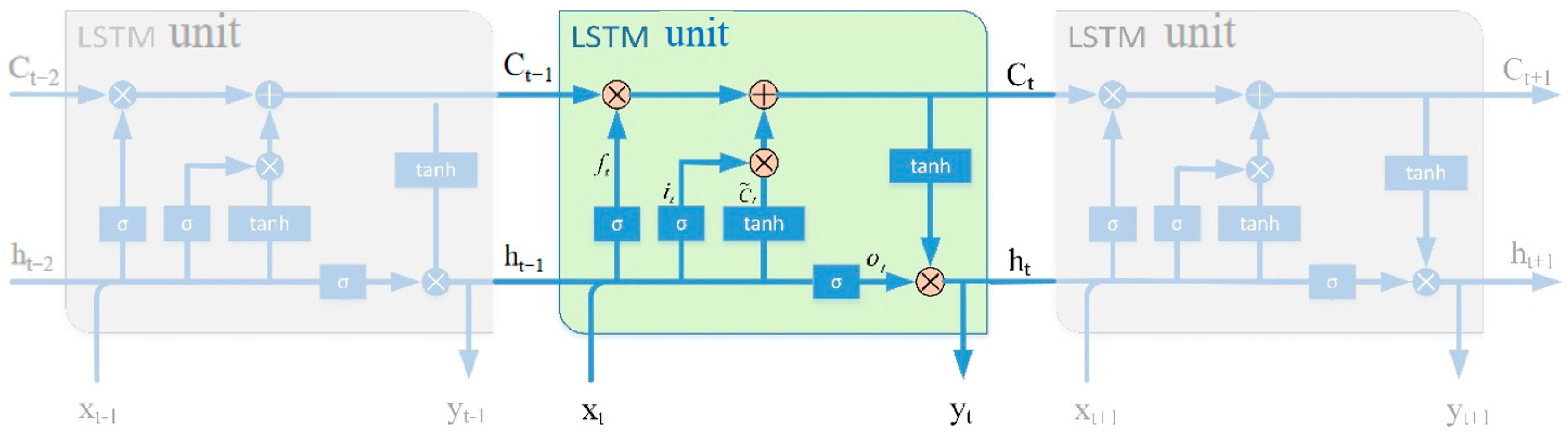
The RNN is a neural network that is good at processing non-linear time series data. However, when dealing with long-term dependencies, recurrent neural networks are prone to falling into gradient vanishing and exploding gradient problems. Therefore, Hochreiter and Schmidhuber [27] proposed the long-term short-term memory neural network (long short-term memory, LSTM). LSTM is a variant of RNN, whose storage unit consists of input gate, output gate, and forgetting gate, where the input gate selectively updates new information to the current unit state, the forgetting gate selectively discards information about the current unit state, and the output gate selectively outputs the result. This structure ensures that the LSTM can determine which units are inhibited or activated based on the state of the previous cell, the state currently stored in, and the current input. The structure of the LSTM is shown in Figure 1, which can effectively overcome the vanishing gradient problem, thus ensuring that the neural network can remember long time series information.
The calculation formula between the variables is as follows:
where , , , represents the weight matrix, , , , denotes the bias vector.
2.1.3. Gate Recurrent Unit (GRU) Neural Network
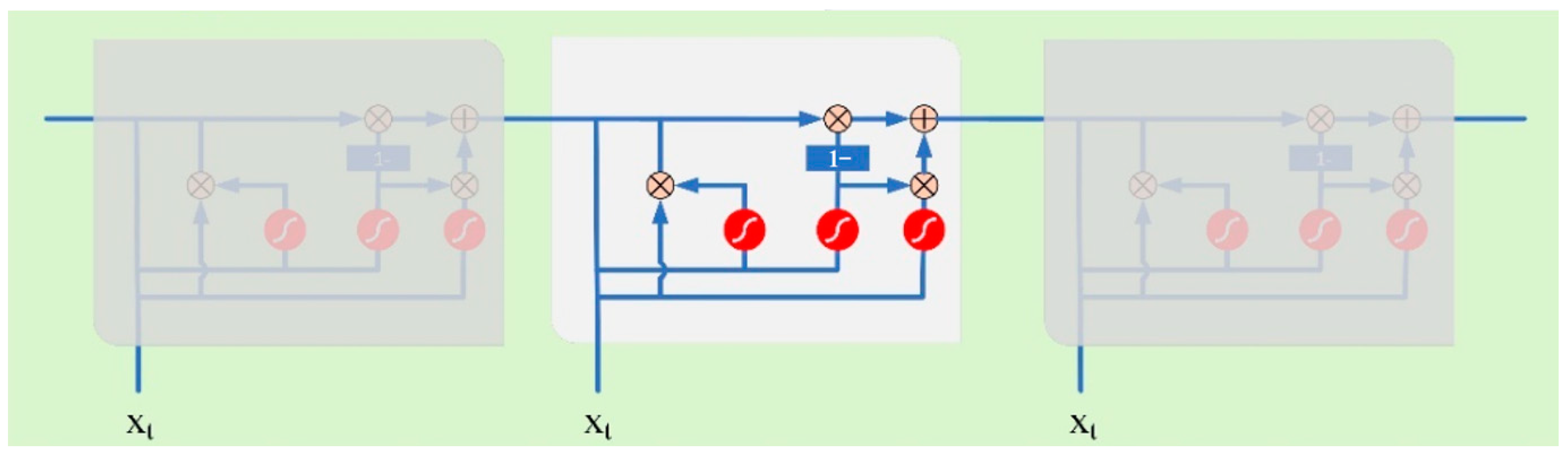
The gate recurrent unit (GRU) is a neural network model proposed by Cho [28] in 2014 to solve long-term dependencies in time series. The GRU network can be seen as a very effective variant of the LSTM network which has a simpler structure and faster training rate. Therefore, the GRU model has been widely used in the field of artificial intelligence, especially in processing time series. The LSTM introduces three gate functions of input gate, forgetting gate, and output gate to control the input value, stored value, and output value, while in the GRU model, it is simplified to two gates which are the update gate and the reset gate. The specific structure of the GRU is shown in Figure 2.
The calculation formula between the variables is as follows:
where, and denotes the weight of the reset gate, and represent the weight of the update gate, and represent the weight of the current memory unit, represent the Hadamard product, represent the sigmoid activation function, and represent the hyperbolic tangential activation function.
2.1.4. The Back Propagation (BP) Neural Network
The BP (back propagation) neural network is a multilayer feedforward network trained by an error backpropagation algorithm proposed by a group of scientists led by Rumelhart and McCelland [29], which is one of the most widely used neural network models at present. The BP neural network does not need to describe the complex relationship between input and output data in advance. The BP neural network provides a large number of input-output patterns, and the model automatically learns and continuously adjusts the weights and thresholds of the network by back-propagation to finally explore the potentially complex relationship between the data, and the structure of the BP neural network is shown in Figure 3.
2.1.5. Multiple Linear Regression (MLR)
Multiple linear regression (MLR) is used to describe the mapping relationship in which the dependent variable depends on the influence of multiple independent variables [30].
The multiple linear regression equation is expressed as
where, is the constant term, is the partial regression coefficient of the independent variable , and is the residual vector.
The above formula can be expressed as a matrix form:
where y is the vector of observed values, X is the matrix of independent variables, the coefficient vector, and the residual vector.
The objective function of the multiple linear regression is the minimum sum of residual squares:
Assuming that X is fully implemented, the final expression of the coefficient vector can be obtained as
2.1.6. Support Vector Regression (SVR)
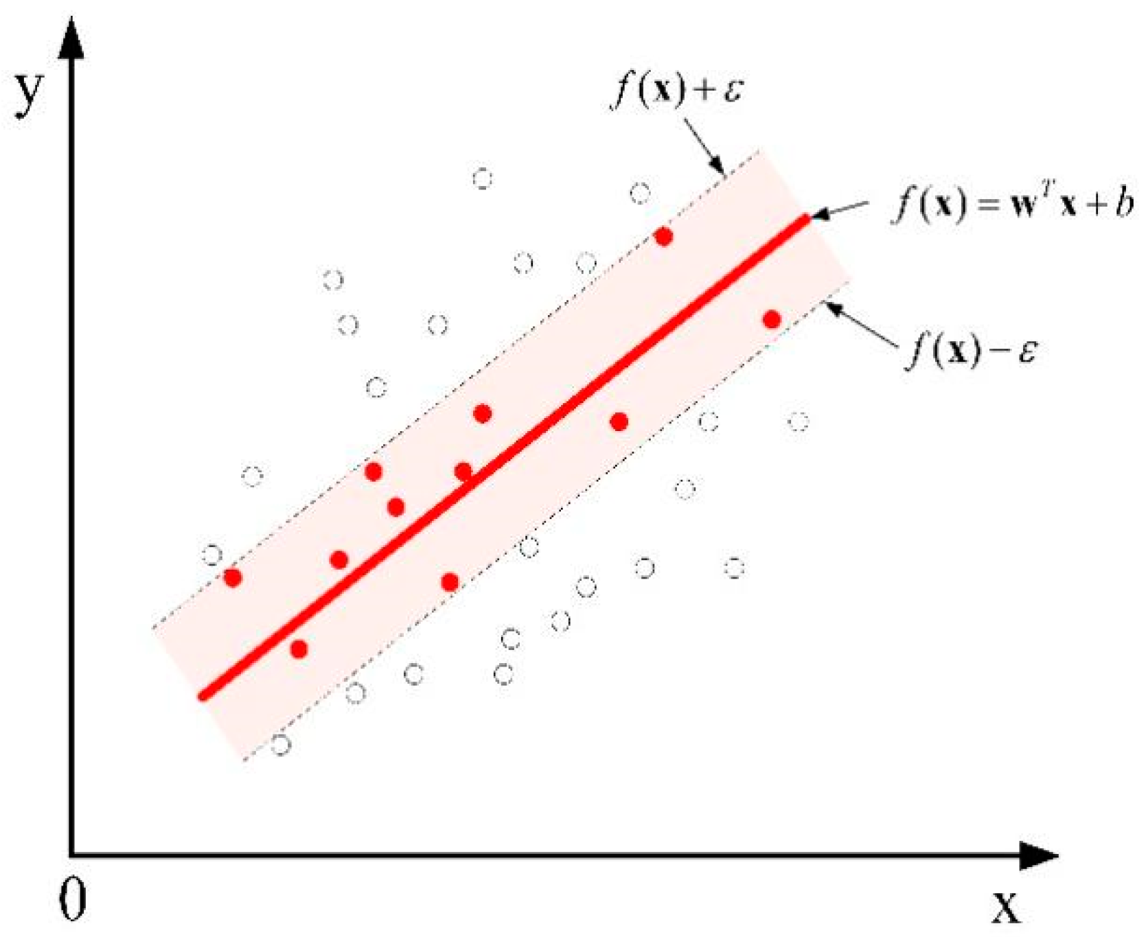
Support vector regression (SVR) is a regression form of support vector machine SVM, which aims to map the input sample data into a high-dimensional feature space by a nonlinear mapping function, and then construct a linear regression problem in this high-dimensional feature space for a solution [31]. Traditional regression models usually treat the error between the output value of the model and the observed value as the loss function. In SVR, an insensitive loss factor is introduced, as shown in Figure 4, and no loss is calculated when the model output samples fall in the red interval band.
2.1.7. Random Forest Regression (RFR)
Random forests [32] are combinations of decision trees that join many decision trees together to reduce the risk of overfitting. Based on the construction of bagging integration with decision trees for machine learning, random forest further introduces random attribute selection in the training process of decision trees. random forest regression (random forest regression) [33] is an important application branch of random forest. The random forest regression model works through the random sampling and features and the establishment of several unrelated decision trees, as a parallel way to obtain the prediction results. Each decision tree can obtain a prediction result based on the samples and features extracted, and the regression prediction result of the whole forest can be obtained by integrating the results of all trees and taking the average value.
2.1.8. AdaBoost Regression (ABR)
The AdaBoost regressor [34] is an ensemble method. The model first uses the original data to fit the regressors, and then uses the same data set to fit multiple regressors, in which the weights of each regressor are adjusted and optimized according to the current predicted errors.
2.2. The Bayesian Model Average (BMA) Method
The Bayesian model average (BMA) [35,36] method is a forecast probabilistic model based on Bayesian statistical theory, which transforms the deterministic forecast provided by a single pattern into the corresponding probability forecast and maximizes the organic combination of data from different sources to make full use of the prediction results of each model. It takes the posterior probability of the observation sample belonging to a certain mode as the weight, and weighted averages over the conditional probability density function of each mode, and then obtains the (posterior) probability density function of the variable. The basic principle is as follows:
The represents the return results of K single modes, y represents the variable to be predicted, then the probability density function (PDF) of the model is:
where wk is the weight, which is also the probability when the kth mode is the best return mode, which is non-negative and satisfies
, reflecting the relative contribution of the kth mode to the prediction technique during the training period. is the conditional probability density function linked to a single pattern return result.
2.3. Hyperparameter Optimization
Hyperparameters are parameters whose values are set before starting the learning process, rather than the parameter data obtained through training. In this paper, the model hyperparameters are optimized using the simulated annealing (SA) algorithm. The essence of the simulated annealing algorithm is to search for the near-optimal solution by using the Metropolis criterion at each value of the decreasing control parameter, and its execution strategy is as follows: the entire solution space is explored starting from any initial solution i. A new solution j is generated by a simple change perturbation, and the Metropolis acceptance criterion is used to determine whether to accept the new solution, and then the control temperature is decremented accordingly, and the above cycle repeated until an approximate optimal solution is found. A brief description of the main steps of the simulated annealing algorithm is given below:
- (1)
- Set the initial temperature, termination temperature and control parameters update function: t0, tf, T(t), which t0 should be sufficiently large, and set the initial value of the cycle counter k = 1.
- (2)
- Generate a random initial state i and use it as the current state to calculate its corresponding objective function value f(i).
- (3)
- Let tk = T(tk−1), given the maximum number of loop steps Lk, the inner loop counter is assigned an initial value of m = 1.
- (4)
- Randomly perturb the current state i, and a new state j is produced after a simple change, then, calculate the value of the objective function f(j) corresponding to j, and calculate the difference of the target function value corresponding to state j and state i.
- (5)
- If f < 0, the newly generated state j is accepted as the current state; conversely, if f ≥ 0, the probability P is used to determine whether state j replaces state i.
Generate a random number ξ on the interval from 0 to 1. If P > ξ, accept the new state j as the initial point for the next determination; otherwise, discard state j and still use state i as the initial point for the next determination.
- (6)
- If m < Lk, then let m = m + 1 and turn to step (4).
- (7)
- If tk > tf, then let k = k + 1 and turn to step (3); if tk ≤ tf, then output the current state and the algorithm ends.
2.4. Overall Process of the Proposed Model
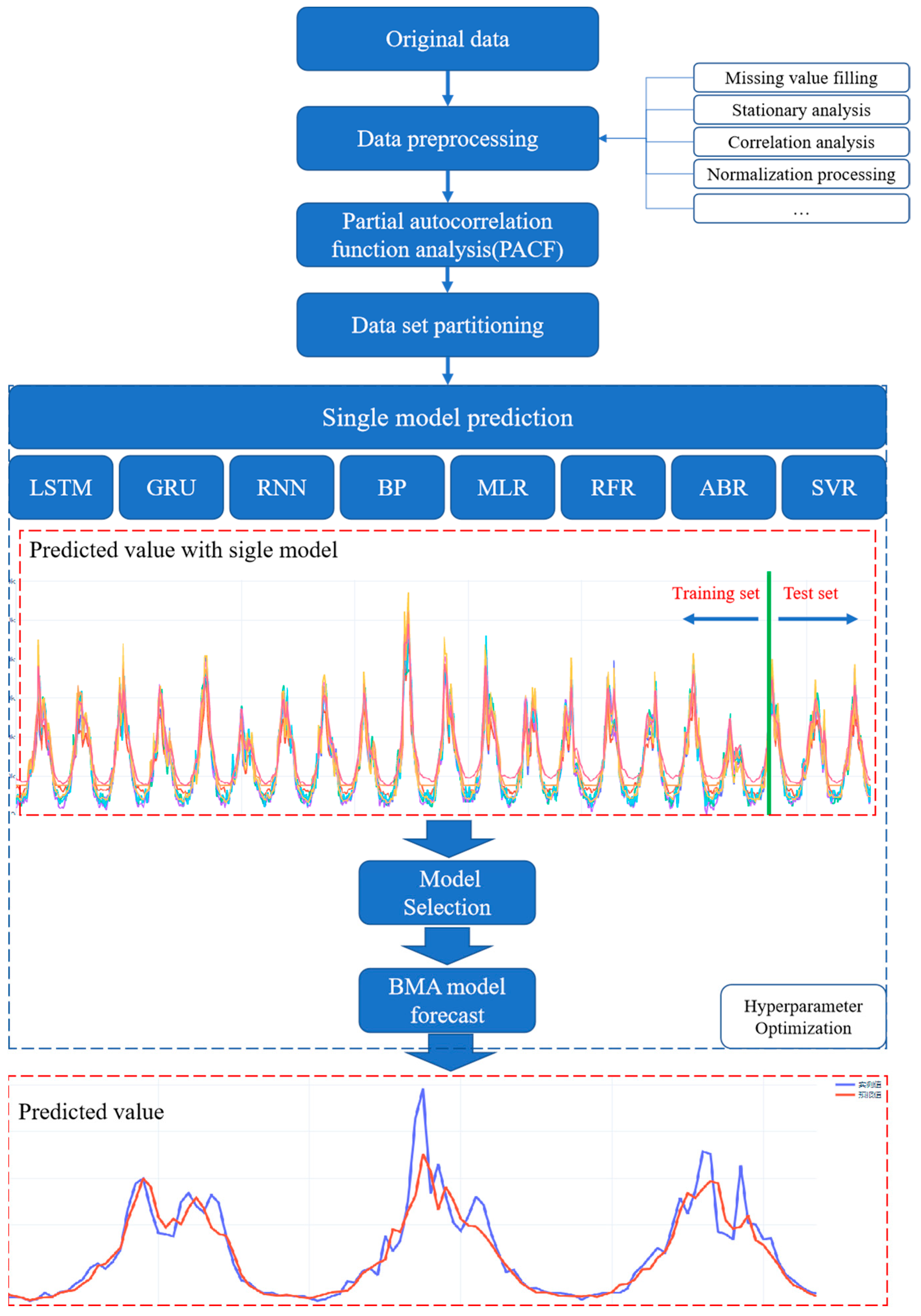
In this paper, a Bayesian model average integrated prediction method is proposed, which combines artificial intelligence algorithms including LSTM, GRU, RNN, BP, MLR, RFR, ABR, and SVR. The whole process of the proposed model is shown in Figure 5.
The modeling process is as follows:
Step 1: Data preprocessing. First, the Dickey–Fowler test (augmented Dickey–Fuller test, ADF test) is used to detect the stationarity of streamflow series. If the null hypothesis is rejected, where the time series data is unstable, differential processing is used to smooth the data.
where xi+1 and xi represent streamflow data at a time (i + 1) and ith, respectively; Δxj are streamflow data at time j after the first order difference.
Then, the data is normalized to the interval [0,1] to eliminate the effect of physical dimensions on the different types of input samples.
where Xi is the normalized results, xi is the streamflow data at the time i, and xmin and xmax represent the minimum and maximum values of the streamflow sequence, respectively.
Step 2: Data set division. The data set is divided into a single model training set, a single model test set, and then the single model test set is divided into the BMA model training set and the BMA model test set;
Step 3: Single-model prediction. Using single model training set for LSTM, GRU, RNN, BP, MLR, RFR, ABR, and SVR model training, prediction of single model prediction data set;
Step 4: Integrated model prediction. The BMA model is trained by using the BMA model training set divided by the single-model prediction data set, and the final streamflow prediction results are predicted.
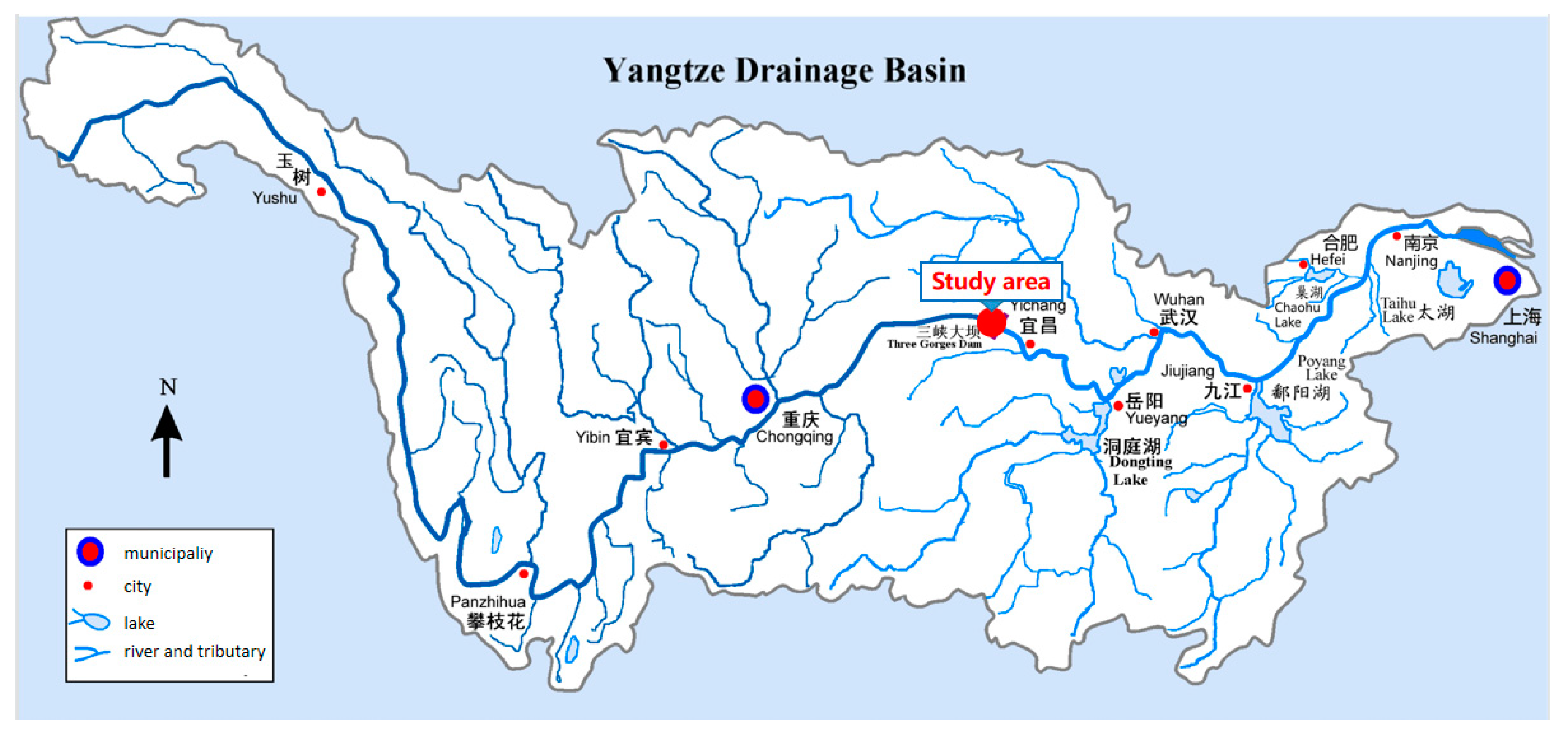
2.5. Study Area
This paper focuses on forecasting the streamflow of the Three Gorges Reservoir. The Three Gorges hydropower station is the control project of the Three Gorges Reservoir, located in Yichang, Hubei Province, China. The flood season of the Three Gorges Reservoir is from May to October. The annual power generation can reach 100 billion kWh, which is equivalent to saving 319 million tons of standard coal and reducing carbon dioxide by 85.8 million tons, bringing huge direct economic benefits. Therefore, it is of great significance to study the streamflow forecast of the Three Gorges Reservoir with regards to reducing flood damage and increasing power generation efficiency.
3. Evaluation Metrics
The root mean square error (RMSE), mean absolute error (MAE), mean absolute percentage error (MAPE), and Nash–Sutcliffe efficiency (NSE) and Pearson correlation coefficient (r) were selected as the evaluation indicators to evaluate the superiority of the model. Each statistical indicator is defined as follows:
where N is the total amount of samples, representing the actual value of the ith sample, the predicted value of the ith sample, and the mean of the sample. Pearson correlation coefficient (r) index is defined as follows:
4. Results and Discussion
In this section, the proposed model is applied to the prediction of the ten-day scale streamflow of the Three Gorges reservoir. To evaluate the reliability of the proposed method, LSTM, GRU, RNN, BP, MLR, RFR, ABR, and SVR were introduced as contrast methods to verify the effectiveness of the proposed method. Meanwhile, RMSE, MAE, MAPE, NSE, and r were introduced to evaluate the prediction results.
4.1. Experimental Date Description
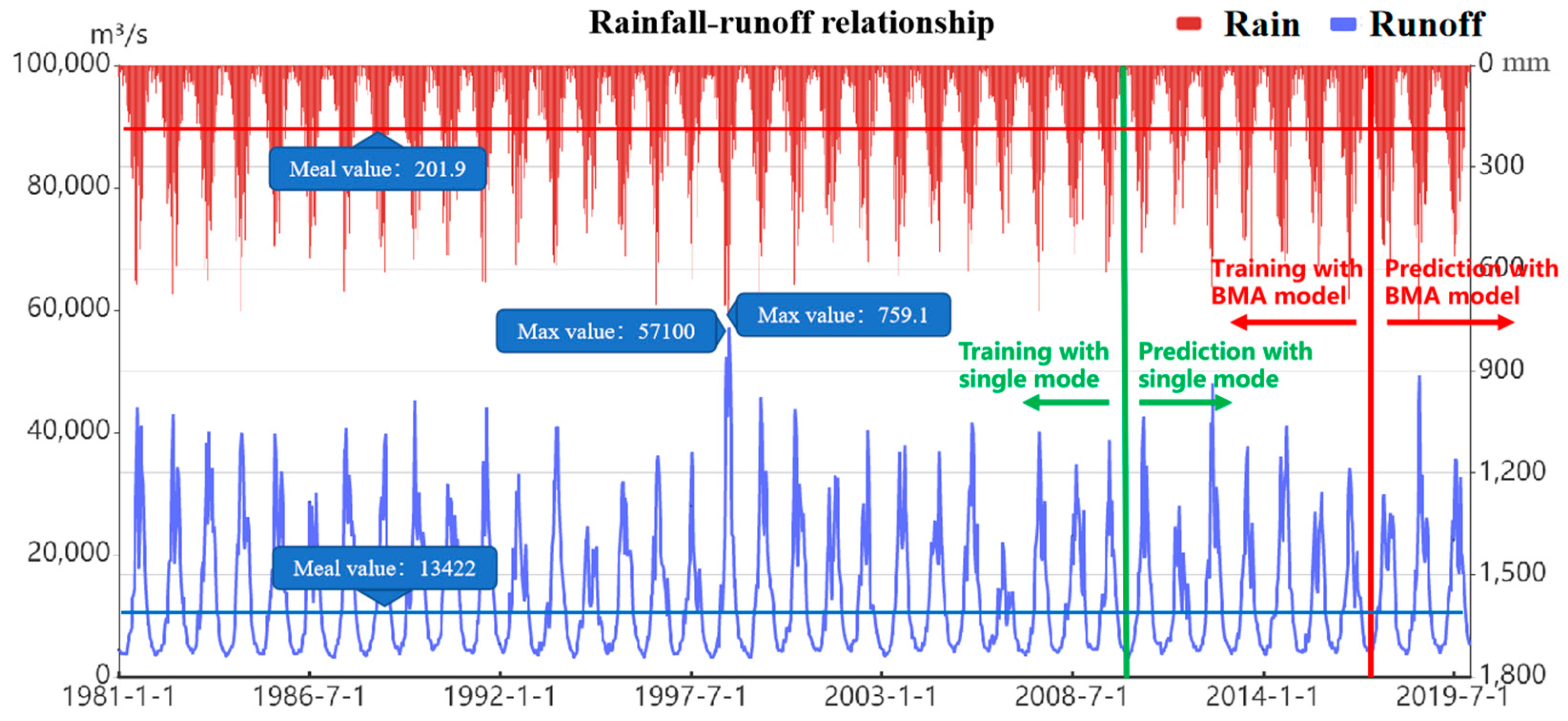
To verify the prediction effect of the model proposed in this paper, case verification and result analysis are carried out by using the 10-day restored streamflow data of the Three Gorges reservoir from 1981 to 2019. The location of study area is shown in Figure 6. The graph of average rainfall and inflow streamflow in the Three Gorges Reservoir area is shown in Figure 7, and the statistical information, including average, maximum, minimum, standard deviation, skewness, kurtosis, and correlation coefficient, are shown in Table 1. The Pearson correlation coefficient of streamflow and rainfall is 0.797, which is highly relevant. Therefore, adding rainfall information in the process of forecasting can improve the accuracy of the model.
According to the modeling process of the multi-model integrated forecasting method mentioned in this paper, the model is first preprocessed, and the linear extrapolation method is used to compensate for the actual data. At the same time, the streamflow data is tested for stability of the data using the augmented Dickey–Fuller test (ADF Test) method. As Table 2 shows, the ADF test results of the Three Gorges Reservoir inflow reduced streamflow are less than 1%, 5%, and 10%, and the p value is close to 0. The test results reject the original assumption that the inflow streamflow time series of the Three Gorges Reservoir is stationary.
4.2. Parameter Selection
In this study, the proposed method and the contrast methods, including LSTM, GRU, RNN, BP, MLR, RFR, ABR, and SVR, are compiled based on Python programming languages, and the TensorFlow-based Keras framework is used to specify the implementation. The hyperparameters, including the number of neural network nodes, the loss function, input dimension m and others, are optimized by a simulated annealing algorithm.
In order to facilitate the optimization of simulated annealing algorithm, the node number range of LSTM, GRU, RNN and BP neural network was set as [5, 30]. Since streamflow has an obvious annual cycle, the range of input dimension m is set as [36, 180], and, because the input data is the average streamflow of 10 days, this means the time span of input streamflow is between 1 year and 5 years.
4.3. Result Analysis and Discussion
In this section, the data from 21 December 1988 to 21 December 2009 are used as the training set for LSTM, GRU, RNN, BP, MLR, RFR, ABR, and SVR models training. The trained models were then used to forecast decadal scale data from 1 January 2010 to 21 December 2019. Through model calculation and parameter optimization, we find that setting the number of nodes of several neural networks as 10 and input dimension as 72 can obtain the optimal prediction results. Compare and analyze the prediction results under different parameters, as shown in Table 3.
As shown in Table 4, when the number of neural network nodes is 10 and the input dimension is 72, the model results are optimal. Therefore, for the well-optimized model, the loss of training process for LSTM, GRU, RNN, and BP neural network is shown in Figure 8. The training set error and test set error are shown in Table 4 and Table 5, respectively.
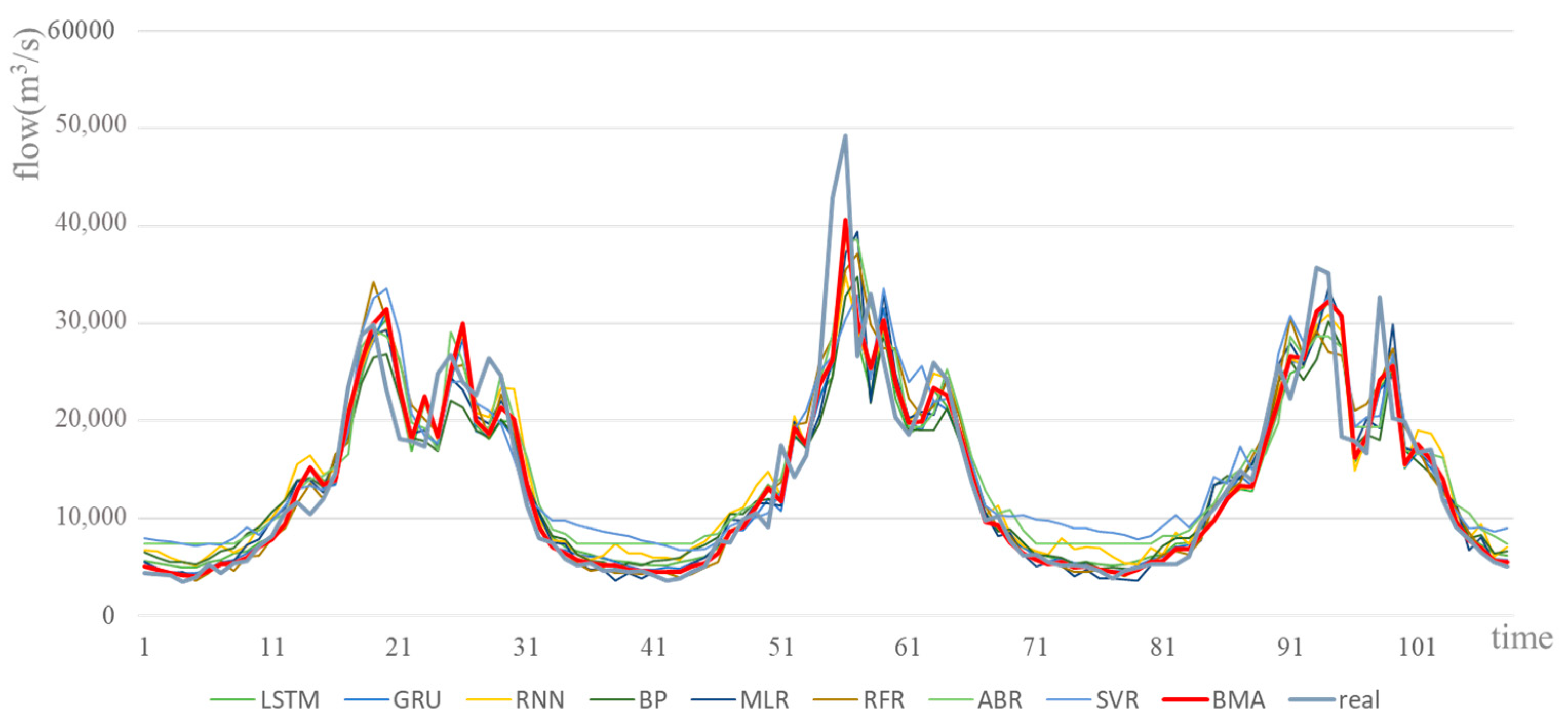
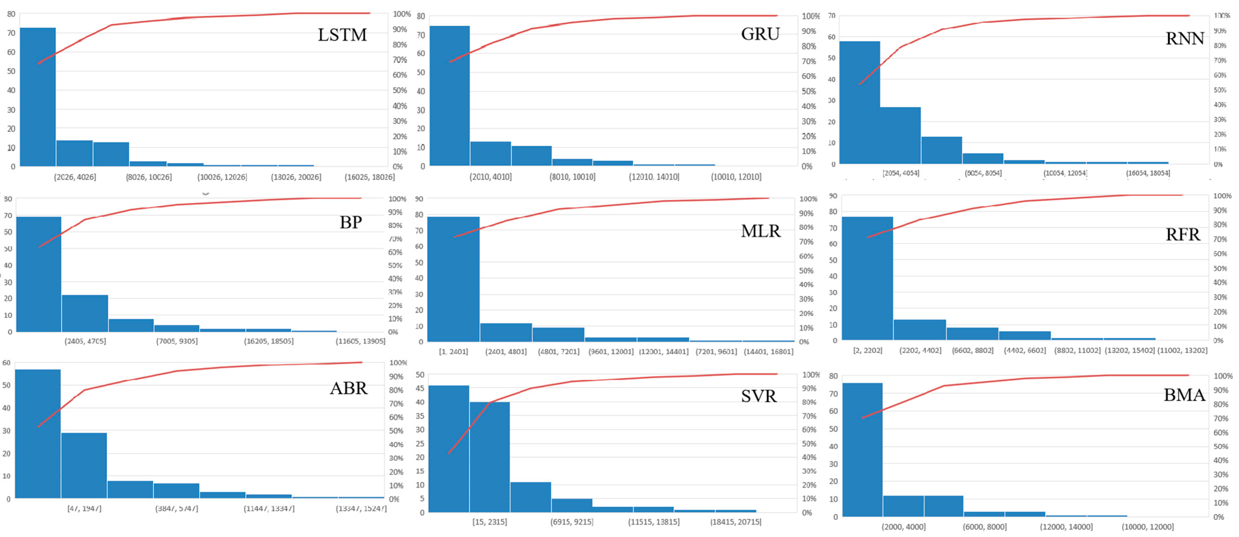
Furthermore, data from 1 January 2010 to 21 December 2019 was divided into a training set (1 January 2010–21 December 2016) and a test set (1 January 2017–21 December 2019) to test the forecasting effect of the BMA model. The models were selected according to the test set forecasting effect, and the better forecasting effect (Pearson correlation coefficient r > 0.8) was selected as the input of the BMA model. The BMA model was trained with data from the training set, and then the streamflow of the Three Gorges reservoir in a ten-day scale from 1 January 2017 to 21 December 2019 is predicted. The comparison of the forecast errors of each model for 1 January 2017–21 December 2019 is shown in Table 6, the comparison of the forecast effects of each model for 1 January 2017–21 December 2019 is shown in Figure 9. and the annual report error distribution for each model 1 January 2017–21 December 2019 is shown in Figure 10.
It can be seen from Figure 9 and Figure 10 and Table 5 and Table 6 that the fitting ability of each single model is different. For a single model, the GRU model has the best prediction effect, with its Nash–Sutcliffe efficiency NSE of 0.871, correlation coefficient r of 0.935, MAPE of 0.142, MAE of 2164, and RMSE of 3491. The SVR model performed the worst, with a Nash–Sutcliffe efficiency NSE of 0.768, a correlation coefficient r of 0.894, a MAPE of 0.37, a MAE of 3474, and a RMSE of 4674. However, after using BMA combined forecasting, the proposed model has the best forecasting effect. The Nash–Sutcliffe efficiency NSE is 0.876, the correlation coefficient r is 0.936, the MAPE is 0.128, the MAE is 2066, and the RMSE is 3416, which shows that the combined model in this paper has better forecasting performance and stronger adaptability.
Furthermore, we separate the flood season and non-flood season for statistical analysis of errors. The Three Gorges Reservoir has a flood season from May to October every year. Therefore, the test set from 2017 to 2019 is divided into flood season and non-flood season for statistical analysis of errors, as shown in Table 7.
As can be seen from the table, the model has a good fitting effect in non-flood season, as the NSE is 0.881, the r is 0.947 and the RMSE is 729. However, the model in flood season has a general fitting effect, where the NSE is 0.646, the r is 0.806 and the RMSE is 4776. Therefore, more relevant information should be further integrated in future studies to improve the forecasting effect in flood season.
In addition, this paper proposed a medium-term streamflow forecasting method, which has achieved good forecasting results. However, the prediction period of this model is only 10 days. Monthly, annual, and longer-term streamflow forecasts are often influenced by global climate factors, such as atmospheric circulation, sea level temperature, and so on. In order to extend the foresight period, it is necessary to further adopt advanced data mining methods to study the impact of various global climate data on medium and long-term streamflow, and then consider global climate data in the input factors of this model to extend the prediction period of the model. This is necessary to provide a basis for water resources management departments to formulate quarterly and annual plans upon.
5. Conclusions
In this study, a Bayesian model average integrated prediction method is proposed, which combines artificial intelligence algorithms including long-and short-term memory neural network (LSTM), gate recurrent unit neural network (GRU), recurrent neural network (RNN), back propagation (BP) neural network, multiple linear regression (MLR), random forest regression (RFR), AdaBoost regression (ABR) and support vector regression (SVR). Notably, the simulated annealing (SA) algorithm is used to optimize the hyperparameters of the model. The following conclusions can be drawn from this study:
- (1)
- Through the application of ten-scale streamflow forecasting in Three Gorges Reservoir. The proposed method has the best performance in the test results of the ten-scale streamflow from the Three Gorges Reservoir from 1 January 2017 to 21 December 2019, with a Nash–Sutcliffe efficiency NSE of 0.876, correlation coefficient r of 0.936, MAPE of 0.128, MAE of 2066, and RMSE of 3416. For the single model, the GRU model has the best prediction effect, and the SVR model performed the worst. The result shows that the proposed method has better forecasting performance compared with a single forecasting model, and the forecasting results can meet the production requirements of water and electricity regulation and other management parts.
- (2)
- By analyzing the prediction results of different hyperparameter models, it can be concluded that the hyperparameter optimization method adopted in this paper can obtain a better set of hyperparameters and has reliability.
- (3)
- By comparing and analyzing the forecasting effect of flood season and non-flood season, we found that the forecasting effect of the model for non-flood season is very good, while the model in flood season has a general fitting effect. Therefore, we suggest that more relevant information should be introduced to further strengthen the study of flood season forecasting.
Author Contributions
Conceptualization, F.H.; methodology, H.Z. and S.C.; software, F.H. and Q.W.; validation, Q.W. and Y.Y.; writing—original draft preparation, F.H.; writing—review and editing, H.Z.; visualization, S.C. and Y.Y.; Data curation, H.Z. and Y.Y. All authors have read and agreed to the published version of the manuscript.
Funding
This work was supported by the Hubei Key Laboratory of Intelligent Yangtze and Hydroelectric Science Open Found (ZH20020001); the National Natural Science Foundation Key Project of China (No. U21A20156); the Central research institutes of basic research and public service special operations (CKSF2021441/SZ); the Hubei natural science foundation (2021CFB151); the Major Science and Technology Projects of Ministry of Water Resources (SKR-2022007); the National Natural Science Foundation of China (No. 51909010); and special thanks are given to the anonymous reviewers and editors for their constructive comments.
Data Availability Statement
The data presented in this study are available on request from the corresponding author. The original data are not publicly available due to the confidentiality agreement with relevant departments.
Acknowledgments
We thank Changjiang Electric Power Company for providing the original data. At the same time, various Python open-source frameworks have been used in this study. We thank all contributors who have made contributions to this.
Conflicts of Interest
The authors declare no conflict of interest.
References
- Devia, G.K.; Ganasri, B.P.; Dwarakish, G.S. A Review on Hydrological Models. Aquat. Procedia 2015, 4, 1001–1007. [Google Scholar] [CrossRef]
- Abbott, M.B.; Bathurst, J.C.; Cunge, J.A.; O’Connell, P.E.; Rasmussen, J. An introduction to the European Hydrological System—Systeme Hydrologique Europeen, “SHE”, 2: Structure of a physically-based, distributed modelling system. J. Hydrol. 1986, 87, 61–77. [Google Scholar] [CrossRef]
- Arnold, J.G.; Srinivasan, R.; Muttiah, R.S.; Williams, J.R. Large area hydrologic modeling and assessment part I: Model development 1. JAWRA J. Am. Water Resour. Assoc. 1998, 34, 73–89. [Google Scholar] [CrossRef]
- Beven, K.J.; Kirkby, M.J. A physically based, variable contributing area model of basin hydrology/Un modèle à base physique de zone d’appel variable de l’hydrologie du bassin versant. Hydrol. Sci. J. 1979, 24, 43–69. [Google Scholar] [CrossRef] [Green Version]
- Sugawara, M.; Watanabe, I.; Ozaki, E.; Katsugama, Y. Tank Model with Snow Component; Research Notes of the National Research Center for Disaster Prevention No. 65; Science and Technolgoy: Ibaraki-Ken, Japan, 1984. [Google Scholar]
- Bergstrom, S. Development and Application of a Conceptual Runoff Model for Scandinavian Catchments; SMHI Norrköping: Norrköping, Switzerland, 1977. [Google Scholar]
- Zang, S.; Li, Z.; Zhang, K.; Yao, C.; Liu, Z.; Wang, J.; Huang, Y.; Wang, S. Improving the flood prediction capability of the Xin’anjiang model by formulating a new physics-based routing framework and a key routing parameter estimation method. J. Hydrol. 2021, 603, 126867. [Google Scholar] [CrossRef]
- Valipour, M.; Banihabib, M.E.; Behbahani, S.M.R. Comparison of the ARMA, ARIMA, and the autoregressive artificial neural network models in forecasting the monthly inflow of Dez dam reservoir. J. Hydrol. 2013, 476, 433–441. [Google Scholar] [CrossRef]
- Besaw, L.E.; Rizzo, D.M.; Bierman, P.R.; Hackett, W.R. Advances in ungauged streamflow prediction using artificial neural networks. J. Hydrol. 2010, 386, 27–37. [Google Scholar] [CrossRef]
- Mouatadid, S.; Adamowski, J. Using extreme learning machines for short-term urban water demand forecasting. Urban Water J. 2017, 14, 630–638. [Google Scholar] [CrossRef]
- Kisi, O. Pan evaporation modeling using least square support vector machine, multivariate adaptive regression splines and M5 model tree. J. Hydrol. 2015, 528, 312–320. [Google Scholar] [CrossRef]
- Castellano-Méndez, M.; González-Manteiga, W.; Febrero-Bande, M.; Manuel Prada-Sánchez, J.; Lozano-Calderón, R. Modelling of the monthly and daily behaviour of the runoff of the Xallas river using Box–Jenkins and neural networks methods. J. Hydrol. 2004, 296, 38–58. [Google Scholar] [CrossRef]
- Niu, W.; Feng, Z.; Cheng, C.; Zhou, J. Forecasting daily runoff by extreme learning machine based on quantum-behaved particle swarm optimization. J. Hydrol. Eng. 2018, 23, 04018002. [Google Scholar] [CrossRef]
- Adnan, R.M.; Liang, Z.; Trajkovic, S.; Zounemat-Kermani, M.; Li, B.; Kisi, O. Daily streamflow prediction using optimally pruned extreme learning machine. J. Hydrol. 2019, 577, 123981. [Google Scholar] [CrossRef]
- Noorbeh, P.; Roozbahani, A.; Kardan Moghaddam, H. Annual and monthly dam inflow prediction using Bayesian networks. Water Resour. Manag. 2020, 34, 2933–2951. [Google Scholar] [CrossRef]
- Costa Silva, D.F.; Galvão Filho, A.R.; Carvalho, R.V.; de Souza, L.; Ribeiro, F.; Coelho, C.J. Water Flow Forecasting Based on River Tributaries Using Long Short-Term Memory Ensemble Model. Energies 2021, 14, 7707. [Google Scholar] [CrossRef]
- Dai, Z.; Zhang, M.; Nedjah, N.; Xu, D.; Ye, F. A Hydrological Data Prediction Model Based on LSTM with Attention Mechanism. Water 2023, 15, 670. [Google Scholar] [CrossRef]
- He, F.; Zhou, J.; Feng, Z.; Liu, G.; Yang, Y. A hybrid short-term load forecasting model based on variational mode decomposition and long short-term memory networks considering relevant factors with Bayesian optimization algorithm. Appl. Energy 2019, 237, 103–116. [Google Scholar] [CrossRef]
- He, F.; Zhou, J.; Mo, L.; Feng, K.; Liu, G.; He, Z. Day-ahead short-term load probability density forecasting method with a decomposition-based quantile regression forest. Appl. Energy 2020, 262, 114396. [Google Scholar] [CrossRef]
- Hou, T.; Fang, R.; Tang, J.; Ge, G.; Yang, D.; Liu, J.; Zhang, W. A Novel Short-Term Residential Electric Load Forecasting Method Based on Adaptive Load Aggregation and Deep Learning Algorithms. Energies 2021, 14, 7820. [Google Scholar] [CrossRef]
- Acaroğlu, H.; García Márquez, F.P. Comprehensive Review on Electricity Market Price and Load Forecasting Based on Wind Energy. Energies 2021, 14, 7473. [Google Scholar] [CrossRef]
- Wang, Y.; Zou, R.; Liu, F.; Zhang, L.; Liu, Q. A review of wind speed and wind power forecasting with deep neural networks. Appl. Energy 2021, 304, 117766. [Google Scholar] [CrossRef]
- Malik, P.; Gehlot, A.; Singh, R.; Gupta, L.R.; Thakur, A.K. A review on ANN based model for solar radiation and wind speed prediction with real-time data. Arch. Comput. Method. E 2022, 29, 1–19. [Google Scholar] [CrossRef]
- Ahmad, N.; Ghadi, Y.; Adnan, M.; Ali, M. Load forecasting techniques for power system: Research challenges and survey. IEEE Access 2022, 10, 71054–71090. [Google Scholar] [CrossRef]
- Wu, Z.; Lu, C.; Sun, Q.; Lu, W.; He, X.; Qin, T.; Yan, L.; Wu, C. Predicting Groundwater Level Based on Machine Learning: A Case Study of the Hebei Plain. Water 2023, 15, 823. [Google Scholar] [CrossRef]
- Hassoun, M.H. Fundamentals of Artificial Neural Networks; MIT Press: Cambridge, MA, USA, 1995. [Google Scholar]
- Hochreiter, S.; Schmidhuber, J. Long Short-Term Memory. Neural Comput. 1997, 9, 1735–1780. [Google Scholar] [CrossRef]
- Cho, K.; Van Merriënboer, B.; Bahdanau, D.; Bengio, Y. On the properties of neural machine translation: Encoder-decoder approaches. arXiv 2014, arXiv:1409.1259. [Google Scholar]
- LeCun, Y.; Touresky, D.; Hinton, G.; Sejnowski, T. A theoretical framework for back-propagation. In Proceedings of the 1988 Connectionist Models Summer School; Morgan Kaufmann: Pittsburgh, PA, USA, 1988; pp. 21–28. [Google Scholar]
- Uyanık, G.K.; Güler, N. A study on multiple linear regression analysis. Procedia-Soc. Behav. Sci. 2013, 106, 234–240. [Google Scholar] [CrossRef] [Green Version]
- Smola, A.J.; Schölkopf, B. A tutorial on support vector regression. Stat. Comput. 2004, 14, 199–222. [Google Scholar] [CrossRef] [Green Version]
- Breiman, L. Random forests. Mach. Learn. 2001, 45, 5–32. [Google Scholar] [CrossRef] [Green Version]
- Segal, M.R. Machine Learning Benchmarks and Random Forest Regression; UCSF: Center for Bioinformatics and Molecular Biostatistics: San Francisco, CA, USA, 2004. [Google Scholar]
- Zhu, X.; Zhang, P.; Xie, M. A Joint Long Short-Term Memory and AdaBoost regression approach with application to remaining useful life estimation. Measurement 2021, 170, 108707. [Google Scholar] [CrossRef]
- Raftery, A.E.; Madigan, D.; Hoeting, J.A. Bayesian model averaging for linear regression models. J. Am. Stat. Assoc. 1997, 92, 179–191. [Google Scholar] [CrossRef]
- Wasserman, L. Bayesian model selection and model averaging. J. Math. Psychol. 2000, 44, 92–107. [Google Scholar] [CrossRef] [PubMed] [Green Version]
Figure 1.
LSTM unit structure schematic.

Figure 2.
GRU unit structure schematic.

Figure 3.
BP neural network structure diagram.

Figure 4.
Schematic diagram of support vector regression hyperplane.

Figure 5.
The whole process of the proposed model.

Figure 6.
Study area.

Figure 7.
Average rainfall and streamflow of the Three Gorges Reservoir.

Figure 8.
Plot of the training process loss of the LSTM, GRU, RNN, and BP neural network models.

Figure 9.
Comparison of the forecast effect of each model for 1 January 2017–21 December 2019.

Figure 10.
Forecast error distribution for each model 1 January 2017–21 December 2019.


Table 1.
Statistical table of inflow and rainfall sequence in the Three Gorges Reservoir.
| Period | Date Range | Mean | Max. | Min. | SD | Skew. | Kurt. | Correlation Coefficent |
|---|---|---|---|---|---|---|---|---|
| Runoff | 1 January 2010–21 December 2019 | 13422 | 57100 | 3040 | 9996.9 | 1.14 | 0.80 | 0.797 |
| Rain | 1 January 2010–21 December 2019 | 201.9 | 759.1 | 1.3 | 173.7 | 0.79 | −0.35 |
Table 2.
The ADF test results for test period.
| Sequence | Date Range | Test Result | p-Value | 1% | 5% | 10% |
|---|---|---|---|---|---|---|
| Inflow | 1981–2021 | −14.767 | 2.356 × 10⁻²⁷ | −3.435 | −2.864 | −2.568 |
Table 3.
Comparison of prediction results of different model parameters.
| Index | Number of Neural Network Nodes | Input Dimension m | MAE | MAPE | RMSE | r | NSE |
|---|---|---|---|---|---|---|---|
| 1 | 10 | 36 | 2099 | 0.130 | 12,018,323 | 0934 | 0.872 |
| 2 | 20 | 72 | 2079 | 0.132 | 11,937,780 | 0.935 | 0.873 |
| 3 | 30 | 72 | 2098 | 0.137 | 12,180,883 | 0.934 | 0.871 |
| 4 | 10 | 72 | 2050 | 0.128 | 11,691,335 | 0.936 | 0.876 |
Table 4.
Statistical table of the prediction error of single model training set.
| Date Range | Error | LSTM | GRU | RNN | BP | MLR | RFR | ABR | SVR |
|---|---|---|---|---|---|---|---|---|---|
| 1 December 1988–21 December 2009 | MAE | 1956 | 1904 | 2368 | 2735 | 2449 | 886 | 3185 | 3396 |
| MAPE | 0.158 | 0.135 | 0.222 | 0.225 | 0.177 | 0.056 | 0.381 | 0.418 | |
| RMSE | 3055 | 3045 | 3508 | 4143 | 3842 | 1486 | 3668 | 3960 | |
| r | 0.964 | 0.965 | 0.958 | 0.928 | 0.929 | 0.990 | 0.956 | 0.946 | |
| NSE | 0.913 | 0.914 | 0.886 | 0.841 | 0.863 | 0.979 | 0.875 | 0.854 |
Table 5.
Statistical table of the prediction error of single model text set.
| Date Range | Error | LSTM | GRU | RNN | BP | MLR | RFR | ABR | SVR |
|---|---|---|---|---|---|---|---|---|---|
| 1 January 2010–21 December 2019 | MAE | 2064 | 1931 | 2497 | 2791 | 2467 | 2258 | 3458 | 3847 |
| MAPE | 0.162 | 0.136 | 0.236 | 0.250 | 0.188 | 0.151 | 0.377 | 0.444 | |
| RMSE | 3160 | 3130 | 3465 | 4136 | 3948 | 3847 | 4450 | 4812 | |
| r | 0.944 | 0.944 | 0.938 | 0.908 | 0.908 | 0.914 | 0.903 | 0.891 | |
| NSE | 0.886 | 0.888 | 0.863 | 0.805 | 0.823 | 0.832 | 0.775 | 0.736 |
Table 6.
Comparison statistics of forecast errors for each model for 2017.1.1–2019.12.21.
| Date Range | Error | LSTM | GRU | RNN | BP | MLR | RFR | ABR | SVR | BMA |
|---|---|---|---|---|---|---|---|---|---|---|
| 1 January 2017–21 December 2019 | MAE | 2333 | 2164 | 2734 | 2758 | 2416 | 2243 | 3197 | 3474 | 2066 |
| MAPE | 0.173 | 0.142 | 0.246 | 0.208 | 0.159 | 0.137 | 0.329 | 0.370 | 0.128 | |
| RMSE | 3625 | 3491 | 3820 | 4210 | 4008 | 3686 | 4119 | 4674 | 3416 | |
| r | 0.931 | 0.935 | 0.928 | 0.912 | 0.911 | 0.925 | 0.920 | 0.894 | 0.936 | |
| NSE | 0.861 | 0.871 | 0.845 | 0.812 | 0.829 | 0.856 | 0.820 | 0.768 | 0.876 |
Table 7.
Comparison of forecast results in flood season and non-flood season.
| Date Range | Season Divided | MAE | MAPE | RMSE | r | NSE |
|---|---|---|---|---|---|---|
| 1 January 2017–21 December 2019 | flood season | 3581 | 0.166 | 4776 | 0.806 | 0.646 |
| non-flood season | 550 | 0.09 | 729 | 0.947 | 0.881 |
Disclaimer/Publisher’s Note: The statements, opinions and data contained in all publications are solely those of the individual author(s) and contributor(s) and not of MDPI and/or the editor(s). MDPI and/or the editor(s) disclaim responsibility for any injury to people or property resulting from any ideas, methods, instructions or products referred to in the content. |
© 2023 by the authors. Licensee MDPI, Basel, Switzerland. This article is an open access article distributed under the terms and conditions of the Creative Commons Attribution (CC BY) license (https://creativecommons.org/licenses/by/4.0/).
Share and Cite
MDPI and ACS Style
He, F.; Zhang, H.; Wan, Q.; Chen, S.; Yang, Y. Medium Term Streamflow Prediction Based on Bayesian Model Averaging Using Multiple Machine Learning Models. Water 2023, 15, 1548. https://doi.org/10.3390/w15081548
AMA Style
He F, Zhang H, Wan Q, Chen S, Yang Y. Medium Term Streamflow Prediction Based on Bayesian Model Averaging Using Multiple Machine Learning Models. Water. 2023; 15(8):1548. https://doi.org/10.3390/w15081548
Chicago/Turabian StyleHe, Feifei, Hairong Zhang, Qinjuan Wan, Shu Chen, and Yuqi Yang. 2023. "Medium Term Streamflow Prediction Based on Bayesian Model Averaging Using Multiple Machine Learning Models" Water 15, no. 8: 1548. https://doi.org/10.3390/w15081548
Note that from the first issue of 2016, this journal uses article numbers instead of page numbers. See further details here.